LRFD Calibration of Axially- Loaded Concrete Piles Driven ... Sean.pdf · LRFD Calibration of...
56
1 LRFD Calibration of Axially-Loaded Concrete Piles Driven into Louisiana Soils Louisiana Transportation Conference February 10, 2009 Sungmin “Sean” Yoon, Ph. D., P.E. (Presenter) Murad Abu-Farsakh , Ph. D., P.E. Ching Tsai, Ph.D., P.E. Zhongjie Zhang, Ph.D., P.E. Louisiana DOTD and LTRC
Transcript of LRFD Calibration of Axially- Loaded Concrete Piles Driven ... Sean.pdf · LRFD Calibration of...

1
LRFD Calibration of Axially-Loaded Concrete Piles Driven into Louisiana
SoilsLouisiana Transportation Conference
February 10, 2009
Sungmin “Sean” Yoon, Ph. D., P.E. (Presenter)Murad Abu-Farsakh , Ph. D., P.E.
Ching Tsai, Ph.D., P.E.Zhongjie Zhang, Ph.D., P.E.
Louisiana DOTD and LTRC

2
Outline
Problem statement Different design methods Statistical concept Methods used in LADOTD for driven piles LRFD calibration Conclusion

3
Problem Statement and Research Objectives
Working Stress Design (WSD) versus LRFD
Bridge super structures vs. Foundation
Federal Highway Administration and ASSHTO set a transition date of October 1, 2007
Resistance Factor (Φ) reflecting Louisiana soil and DOTD design process

4
Stress Design Methodologies vs. LRFD
Working Stress Design (WSD) –also called Allowable Stress Design (ASD), since early 1800s.
where, Q=design load; Qall= allowable design load; and Rn= ultimate resistance of the structure
nall
RQ QFS
≤ = =

5
Stress Design Methodologies vs. LRFD
Limit State Design (LSD), 1950s
Ultimate Limit Stress (ULS)
Service Limit Stress (SLS)
Factored resistance ≥ Factored load effects
Deformation ≤ Tolerable deformation to remain serviceable

6
Stress Design Methodologies vs. LRFD
Load and Resistance Factor Design (LRFD)
where, Φ=resistance factor, Rn=ultimate resistance; γD=load factor for dead load; γL=load factor for live load; γi=corresponding load factor, and Qi=summation of load
n D D L L i iR r Q r Q rQφ ≥ + = ∑

7
Reliability Based FS

8
Working Stress Design (WSD) vs. LRFD

9
Limit State Function
Limit State Function can be defined as g = R – Q

10
Reliability Index, β
βσg β: reliability index
0 gQR =− lnln g
Pf = shaded area
f(g) = probability density of g2 2
R Q
g R Q
g µ µβ
σ σ σ
−= =
+

11
Relationship between β and Pf
Pf β10-1 1.2810-2 2.3310-3 3.0910-4 3.7110-5 4.2610-6 4.7510-7 5.1910-8 5.6210-9 5.99

12
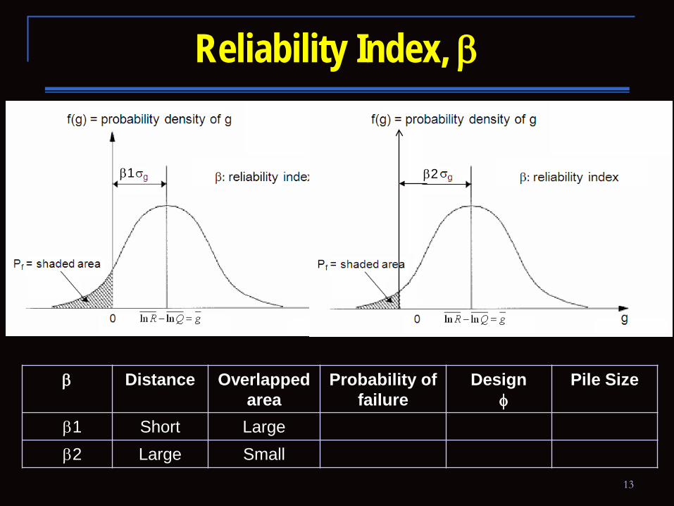
Reliability Index, β
β2β1
β Distance Overlapped area
Probability of failure
Design �φ
Pile Size
�β1 Short�β2 Large
13
Reliability Index, β
β2β1
β Distance Overlapped area
Probability of failure
Design �φ
Pile Size
�β1 Short Large�β2 Large Small

14
Reliability Index, β
β2β1
β Distance Overlapped area
Probability of failure
Design �φ
Pile Size
�β1 Short Large High�β2 Large Small Low

15
Reliability Index, β
β2β1
β Distance Overlapped area
Probability of failure
Design �φ
Pile Size
�β1 Short Large High Large�β2 Large Small Low Small

16
Reliability Index, β
β2β1
β Distance Overlapped area
Probability of failure
Design �φ
Pile Size
�β1 Short Large High Large Small�β2 Large Small Low Small Big

17
How to Treat Uncertainty
1 2
Graph Variability Overlapped area
Probability of failure
Calculated φ
Pile Size
12

18
How to Treat Uncertainty
1 2
Graph Variability Overlapped area
Probability of failure
Calculated φ
Pile Size
1 Low2 High

19
How to Treat Uncertainty
1 2
Graph Variability Overlapped area
Probability of failure
Calculated φ
Pile Size
1 Low Small2 High Large

20
How to Treat Uncertainty
1 2
Graph Variability Overlapped area
Probability of failure
Calculated φ
Pile Size
1 Low Small Low2 High Large High

21
How to Treat Uncertainty
1 2
Graph Variability Overlapped area
Probability of failure
Calculated φ
Pile Size
1 Low Small Low Large2 High Large High Small

22
How to Treat Uncertainty
1 2
Graph Variability Overlapped area
Probability of failure
Calculated φ
Pile Size
1 Low Small Low Large Small2 High Large High Small Big
23
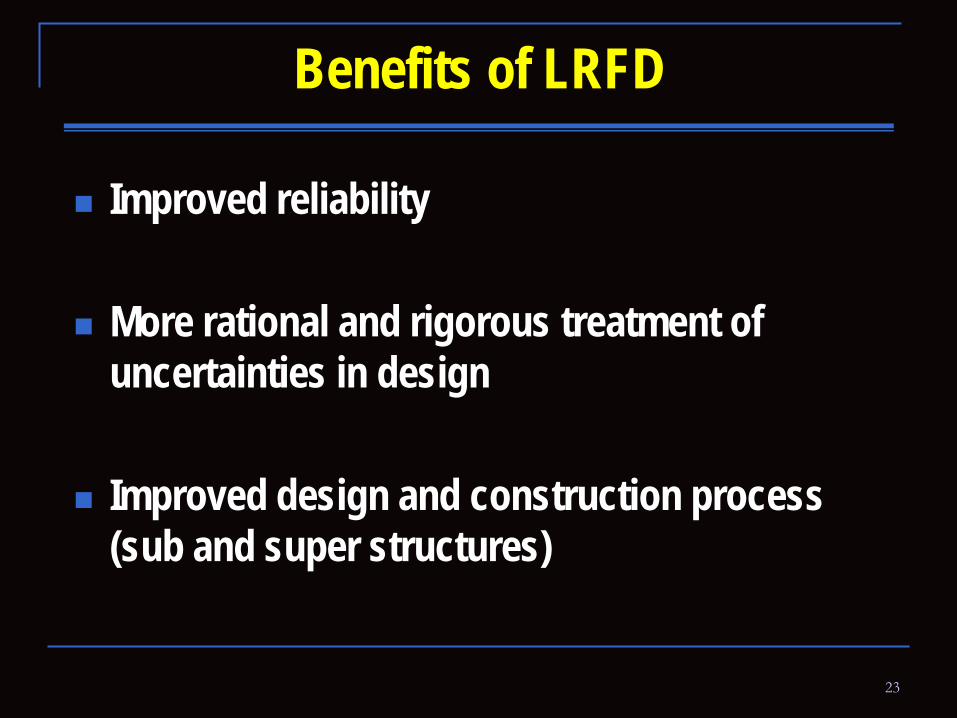
Benefits of LRFD
Improved reliability
More rational and rigorous treatment of uncertainties in design
Improved design and construction process (sub and super structures)

24
First Order Second Moment (FOSM)
Load and Resistance Factor Design (LRFD)
(1)
where, Φ=resistance factor, Rn=ultimate resistance; γD=load factor for dead load; γL=load factor for live load; γi=corresponding load factor, and Qi=summation of load
n D D L L i iR r Q r Q rQφ ≥ + = ∑

25
First Order Second Moment (FOSM)
(2)
Combining eq (1) and (2) using Rn
λQD, λQL = dead and live load bias factors
λR = resistance bias factors = Rm/Rp
AASHTO LRFD specification (1994)
λQD=1.08, λQL=1.15, rD=1.25, rL=1.75, COVQD=0.13, COVQL=0.18
( )( )[ ]2LL
2DL
2R
2R
2LL
2DL
2R
LLLL
DLDL
LL
DL
R
COVCOV1COV1ln
COV1COVCOVCOV1
λQQλ
1QQ
FSλln
β+++
++++
+
+
=
( )( )[ ]( )2QL
2QD
2RTQL
L
DQD
2R
2QL
2QD
LL
DDR
COV+COV+1COV+1lnβexpλ+QQλ
COV+1COV+COV+1
γ+QQγλ
=
φ

26
Statistical Methods for LRFD Calibration
First Order Second Moment (FOSM) method: Linearization of limit state function by expanding Taylor series
expansion First Order Reliability Method (FORM):
Transformation of variables into the standardized and uncorrelated normal variables using the Hosofer-Lind Transformation
Monte Carlo Simulation Method: Extrapolate CDF for each random variable using random number
generator

27
Pile Load Test Database(Ultimate Capacity for Driven Piles)
Square PPC Pile Size (mm)
Pile Type Predominant Soil Type
Friction End-Bearing
Cohesi-ve
Cohesi-onless
Limit of Informa
-tion
360 18 0 16 2 0
410 5 0 3 0 2
610 9 0 6 3 0
760 10 0 5 5 0
Total 42 0 30 10 2

28
Methods used in LADOTD(Ultimate Capacity for Driven Piles)
Static method α - method - for cohesive soil (Tomlison 1979) Nordlund method – for sand inter-layers
CPT method Schmertmann, LCPC, De Ruiter and Beringen
Dynamic Measurement CAPWAP
Measured Ultimate Pile Capacity Butler-Hoy Method Davisson Method

29
Davisson (Interpretation of Pile Load Tests)Static Load Test Results
0.00
0.50
1.00
1.50
2.00
2.50
0 50 100
Load (Tons)Se
ttlem
ent (
in)
Qult
L/AE1
0.15+D/120
30
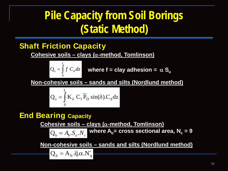
Pile Capacity from Soil Borings (Static Method)
Shaft Friction CapacityCohesive soils – clays (α-method, Tomlinson)
where f = clay adhesion = α Su
Non-cohesive soils – sands and silts (Nordlund method)
End Bearing CapacityCohesive soils – clays (α-method, Tomlinson)
where Ab= cross sectional area, Nc = 9
Non-cohesive soils – sands and silts (Nordlund method)
∫=L
d dzCf0
s Q
∫ δ= δ
L
0dDfs dzC).sin(PC KQ
qbb N..q.AQ ′α=
cub NSA ..Qb =

31
Ultimate Pile Capacity
End-bearing Capacity, Qtip= qt . At
Shaft friction Capacity, Qshaft = Σfi . Asi
Qult = Qtip + Qshaft
f
qt

32
Cone Penetration Test (CPT/PCPT)
qc
fs
U3
U2U1
Penetration Rate = 2 cm/sBase area = 10 cm2
Sleeve area = 150 cm2
Cone angle = 60o

33
Cone Penetrometer Versus Pile
qc
f s
f
qt
Qult
Due to similarity between the cone and pile, the cone can be considered as a simple mini pile.
fs can be correlated to f, qc can be correlated to qt.

34
Typical PCPT Test Results
qc
fs
U3
U2U1
0
1
2
3
4
5
6
7
8
9
10
11
12
13
14
15
16
Dept
h (m
)
0 2 4 6 8 10Tip Resistance (MPa)
0123456789
10111213141516
0.00 0.05 0.10 0.15Sleeve Friction (MPa)
0123456789
10111213141516
0 2 4 6 8Rf (%)
0123456789
10111213141516
0.0 0.1 0.2 0.3 0.4 0.5Pore Pressure (MPa)
Tip
Base
u1
u2
%100qfR
c
sf =

35
Schmertmann method (CPT)
where,qt: unit bearing capacity of
pilef: unit skin frictionαc: reduction factor (0.2 ~
1.25 for clayey soil)fs: sleeve friction
e
D
a
bb
Envelope of minimum qc values yD
?
'x'
8D
Cone resistance qc
Dept
h
qc1 + qc2
2
c
qc1
qc2
qt =

36
LCPC method (CPT)
Pile
a=1.5 D
0.7qcaqca 1.3qca
qc
Dept
ha
a
qeq
Dqt = kb qeq (tip)
kb = 0.6 clay-silt0.375 sand-gravel
maxs
eq k(side)/q
ff <=
ks = 30 to 150

37
De Ruiter and Beringen (CPT) In clay
Su(tip) = qc(tip) / Nk Nk = 15 to 20 qt = Nc.Su(tip) Nc = 9 f = β.Su(side) β = 1 for NC clay
= 0.5 for OC clay In sand
qt similar to Schmertmann method
=
TSF21tension400side
ncompressio300sideiction)(sleeve fr
. )( /)(q
)( /)(q f
minfc
c
s

38
Implementation into a Computer Program
Louisiana Pile Design by Cone Penetration Test
http://www.ltrc.lsu.edu/

39
Predicted vs. Measured Ultimate Pile Resistances
(a) Static analysis method (b) Schmertmann method
0 100 200 300 400 500 600 700 800
Measured pile capacity, Rm (tons)
0
100
200
300
400
500
600
700
800
Pre
dict
ed p
ile c
apac
ity, R
P (t
ons)
RFit = 0.96 * Rm
R2 = 0.87
0 100 200 300 400 500 600 700 800
Measured pile capacity, Rm (tons)
0
100
200
300
400
500
600
700
800
Pre
dict
ed p
ile c
apac
ity, R
P (t
ons)
RFit = 1.12 * Rm
R2 = 0.86

40
Predicted vs. Measured Ultimate Pile Resistances
(c) LCPC method (d) De Ruiter& Beringen method
0 100 200 300 400 500 600 700 800
Measured pile capacity, Rm (tons)
0
100
200
300
400
500
600
700
800
Pre
dict
ed p
ile c
apac
ity, R
P (t
ons)
RFit = 1.07 * Rm
R2 = 0.81
0 100 200 300 400 500 600 700 800
Measured pile capacity, Rm (tons)
0
100
200
300
400
500
600
700
800
Pre
dict
ed p
ile c
apac
ity, R
P (t
ons)
RFit = 0.91 * Rm
R2 = 0.88

41
Predicted vs. Measured Ultimate Pile Resistances
(e) CAPWAP-EOD (f) CAPWAP-14 days BOR
0 100 200 300 400 500 600 700 800
Measured pile capacity, Rm (tons)
0
100
200
300
400
500
600
700
800
Pre
dict
ed p
ile c
apac
ity, R
P (t
ons)
RFit = 0.32 * Rm
R2 = 0.69
0 100 200 300 400 500 600 700 800
Measured pile capacity, Rm (tons)
0
100
200
300
400
500
600
700
800
Pre
dict
ed p
ile c
apac
ity, R
P (t
ons)
RFit = 0.92 * Rm
R2 = 0.91
42
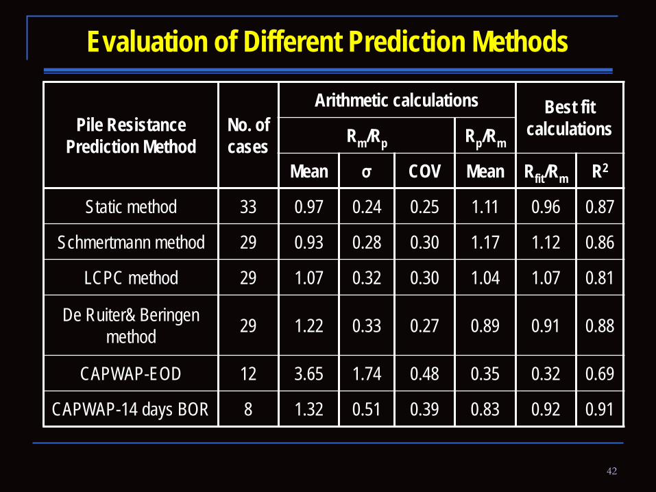
Evaluation of Different Prediction Methods
Pile Resistance Prediction Method
No. of cases
Arithmetic calculations Best fit calculationsRm/Rp Rp/Rm
Mean σ COV Mean Rfit/Rm R2
Static method 33 0.97 0.24 0.25 1.11 0.96 0.87
Schmertmann method 29 0.93 0.28 0.30 1.17 1.12 0.86
LCPC method 29 1.07 0.32 0.30 1.04 1.07 0.81
De Ruiter& Beringen method 29 1.22 0.33 0.27 0.89 0.91 0.88
CAPWAP-EOD 12 3.65 1.74 0.48 0.35 0.32 0.69
CAPWAP-14 days BOR 8 1.32 0.51 0.39 0.83 0.92 0.91

43
Distribution of Bias (Static Analysis)
0.0 0.4 0.8 1.2 1.6 2.0 2.4 2.8 3.2 3.6 4.0
Rm / RP
0
5
10
15
20
25
30
Pro
babi
lity
(%) Log-Normal Distribution
Normal Distribution
Static MethodStatic Method
-3
-2
-1
0
1
2
3
0 0.5 1 1.5 2
Bias, X
Stan
dard
Nor
mal
Var
iabl
e, z
measuredbias value
predictednormaldist.
predictedlognormaldist. fromnormalstat.

44
Distribution of Bias (Schmertmann Method)
0.0 0.4 0.8 1.2 1.6 2.0 2.4 2.8 3.2 3.6 4.0
Rm / RP
0
5
10
15
20
25
30
Pro
babi
lity
(%) Normal Distribution
Log-Normal Distribution
Schmertmann Method Schmertmann Method
-3
-2
-1
0
1
2
3
0 0.5 1 1.5 2
Bias, X
Stan
dard
Nor
mal
Var
iabl
e, z
measuredbias value
predictednormaldist.
predictedlognormaldist. fromnormalstat.

45
Distribution of Bias (LCPC method)
0.0 0.4 0.8 1.2 1.6 2.0 2.4 2.8 3.2 3.6 4.0
Rm / RP
0
5
10
15
20
25
30
Pro
babi
lity
(%) Log-Normal Distribution
Normal Distribution
LCPC Method LCPC Method
-3
-2
-1
0
1
2
3
0 0.5 1 1.5 2
Bias, X
Stan
dard
Nor
mal
Var
iabl
e, z
measuredbias value
predictednormaldist.
predictedlognormaldist. fromnormalstat.

46
Distribution of Bias (De Ruiter& Beringen Method)
0.0 0.4 0.8 1.2 1.6 2.0 2.4 2.8 3.2 3.6 4.0
RP / Rm
0
5
10
15
20
25
30
Pro
babi
lity
(%) Log-Normal Distribution
Normal Distribution
De Ruiter MethodDe Ruiter& Beringen Method
-3
-2
-1
0
1
2
3
0 0.5 1 1.5 2
Bias, X
Stan
dard
Nor
mal
Var
iabl
e, z
measuredbias value
predictednormaldist.
predictedlognormaldist. fromnormalstat.
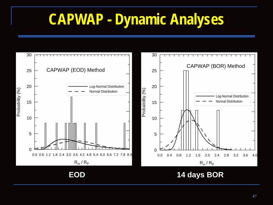
47
CAPWAP - Dynamic Analyses
0.0 0.6 1.2 1.8 2.4 3.0 3.6 4.2 4.8 5.4 6.0 6.6 7.2 7.8 8.4
Rm / RP
0
5
10
15
20
25
30
Pro
babi
lity
(%) Log-Normal Distribution
Normal Distribution
CAPWAP (EOD) Method
0.0 0.4 0.8 1.2 1.6 2.0 2.4 2.8 3.2 3.6 4.0
Rm / RP
0
5
10
15
20
25
30
Pro
babi
lity
(%)
Log-Normal DistributionNormal Distribution
CAPWAP (BOR) Method
EOD 14 days BOR

48
Resistance Factors, φ (Static analysis)
0 0.5 1 1.5 2 2.5 3 3.5 4βT
0
0.5
1
1.5
φ (S
tatic
Ana
lysi
s)

49
Resistance Factors, φ (Direct CPT Methods)
0 0.5 1 1.5 2 2.5 3 3.5 4βT
0
0.5
1
1.5
φ (D
irect
CP
T M
etho
ds)
SchmertmannLCPCDeRuiter&Beringen

50
Resistance Factors, φ (CAPWAP-BOR)
0 0.5 1 1.5 2 2.5 3 3.5 4βT
0
0.5
1
1.5
φ (C
PT
CA
PW
AP
-BO
R A
naly
sis)

51
Resistance Factors, φ (βT=2.33) using FOSM
Design MethodResistance Factor, φ
Efficiency Factor (φ/λ)
Proposed for soft soil
AASHTO Proposed forsoft soil
Static Method α-Tomlinson method and Nordlund method 0.56 0.35 - 0.45 0.58
Direct CPTMethod
Schmertmann 0.48 0.5 0.52
LCPC/LCP 0.56 NA 0.52
De Ruiter and Beringen 0.68 NA 0.55
Dynamicmeasurement
CAPWAP (EOD) 1.31 NA 0.36
CAPWAP (14 days BOR) 0.58 0.65 0.44

52
Comparison of Resistance Factors, φ (βT=2.33) using FOSM, FORM and M-C
Design MethodResistance Factor, φ
FOSM FORM M-C
Static Method α-Tomlinson method and Nordlund method 0.56 0.63 0.63
Direct CPTMethod
Schmertmann 0.48 0.54 0.53
LCPC/LCP 0.56 0.63 0.62
De Ruiter and Beringen 0.68 0.77 0.75
Dynamicmeasurement
CAPWAP (EOD) 1.31 1.41 N/A
CAPWAP (14 days BOR) 0.58 0.63 0.63

53
Conclusions
Preliminary resistance factors (φ) for Louisiana soil were evaluated for different driven pile design methods
Statistical analyses comparing the predicted and measured pile resistances were conducted to evaluate the performance of the different pile design methods.
LRFD in deep foundation can improve its reliability due to more balanced design.
More statistical data is needed for more rational resistance factor.

54
Issues
Load sharing and overall redundancy Reduced φ to reflect increased β
Site variability Based on the filed and laboratory testing Resistance factor and number of static load test
needed
Scour

55
Acknowledgement
The project is financially supported by the Louisiana Transportation Research Center and Louisiana Department of Transportation and Development (LA DOTD).
LTRC Project No. 07-2GT.

56
THANK YOU!
Sungmin “Sean” YoonLADOTD


![[Report] Resistance Factor Calculations for LRFD of Axially Loaded Driven Piles in Sands](https://static.fdocuments.net/doc/165x107/577d1e381a28ab4e1e8e01c5/report-resistance-factor-calculations-for-lrfd-of-axially-loaded-driven-piles.jpg)