)LQLWH (OHPHQW 0RGHOLQJ RI 6NXOO...
70
IN DEGREE PROJECT TECHNOLOGY AND HEALTH, SECOND CYCLE, 30 CREDITS , Finite Element Modeling of Skull Fractures Material model improvements of the skull bone in the KTH FE head model FRIDA ANDERSSON KTH ROYAL INSTITUTE OF TECHNOLOGY SCHOOL OF TECHNOLOGY AND HEALTH
Transcript of )LQLWH (OHPHQW 0RGHOLQJ RI 6NXOO...

INDEGREE PROJECT TECHNOLOGY AND HEALTH,SECOND CYCLE, 30 CREDITS,
Finite Element Modeling of Skull FracturesMaterial model improvements of the skull bone in the KTH FE head modelFRIDA ANDERSSON
KTH ROYAL INSTITUTE OF TECHNOLOGYSCHOOL OF TECHNOLOGY AND HEALTH


This Master’s thesis project was performed at the Department of Neuronics at
KTH Royal Institute of Technology, Stockholm, Sweden
Finite Element Modeling of Skull Fractures- Material model improvements of the skull bone in the
KTH FE head model
Finita Element Modellering av Skallfrakturer- förbättringar av materialmodellen för skallbenet
i KTHs FE skallmodell
FRIDA ANDERSSON
Master of Science Thesis in Medical Engineering
Advanced level (second cycle), 30 credits
Supervisor at STH: Svein Kleiven, Victor Strömbäck Alvarez
Industrial Supervisor: Bengt Pipkorn, Autoliv Development AB
Reviewer: Madelen Fahlstedt
Examiner: Mats Nilsson
School of Technology and Health
TRITA-STH. EX 2016:80
Royal Institute of Technology
KTH STH
SE-141 86 Flemingsberg, Sweden
http://www.kth.se/sth


Abstract
The main aim of this project was to develop a model for predicting skull fractures of a 50th percentile
male, using a finite element head model developed at the Neuronics department of KTH, Royal Institute
of Technology. The skull bone is modeled as a three layered bone, where the outer and inner tables are
modeled as shell elements, while the diploë is modeled by two layers of solid elements. The material
model of the tables was changed from the material model MAT_PLASTIC_KINEMATIC to a material
model including a damage parameter to soften the damaged material and to enable ploting of the damage
of the skull bone. Due to the coarse mesh of the FE head model the material model was not allowed to
include any erosion, deleting element as they reach their ultimate strain. With these requests, two
materials from the LS-DYNA material library seemed appropriate: material 81,
MAT_PLASTICITY_WITH_DAMAGE and material 105 MAT_DAMAGE_2.
To evaluate these materials and adjust the input parameters a dog bone FE model was developed and
tension tests were simulated with this model, equivalent to tension tests performed on equally shaped
skull bone specimens. The material simulating a behavior most similar to the behavior from the tension
tests turned out to be material 81. This material model was then implemented in the full FE head model
for further input parameter adjustment and validation. Four different cadaver experiments were
simulated, with different impacting objects: sphere, box, cylinder and flat cylinder surface, and impacted
areas of the head: vertex, temporo-parietal and frontal. The forces obtained in the simulations were
compared to the forces of the cadaver experiments. The fracture prediction was based on the damage
parameter, which could be plotted to visualize the areas where the ultimate strain was exceeded and
thereby the area most likely to be fractured. This parameter was then compared to the documented
fractures from the cadaver experiments.
The result showed that using material 81 with the input parameter EPPFR=0.05 gave the overall most
accurate forces and fracture predictions. The breaking stress, σB, did not affect the fractures significantly
but a reduced σB resulted in reduction of the peak forces. The thickness of the diploë did not have any
significant impact on the fracture occurrence, but a thinner diploë had a reducing impact on the peak
forces as well.


Sammanfattning
Syftet med projektet presenterat i denna rapport var att utveckla en modell för att möjliggöra modellering
av skallfrakturer för en 50 percentil man. Detta gjordes med hjälp av en huvudmodell av finita element
utvecklad av enheten för Neuronik på Kungliga Tekniska Högskolan. Skallbenet är modellerat i tre lager,
där det yttre och inre kompakta benlagren är modellerade av skalelement medan det porösa benet är
modellerat av två lager solida element. Materialmodellen för det kompakta benet byttes ut från modellens
originalmaterial, MAT_PLASTIC_KINEMATIC till en materialmodell som innefattade en damage-
parameter, vars syfte var att göra materialet mjukare då det börjar plasticera samt möjliggöra
visualisering av denna parameters spridning. På grund av de stora elementen i modellen fick den valda
materialmodellen inte innefatta någon erosion av element, då detta skulle innebära avvikelser av
energibalansen i modellen. För detta hittades två möjliga materialmodeller: material 81,
MAT_PLASTICITY_WITH_DAMAGE och material 105, MAT_DAMAGE_2.
För att utvärdera dessa materialmodeller och anpassa deras olika parametrar var en dogbone-FE modell
utvecklad. Dragprover var sedan simulerade med denna modell, liknande de dragprover som genomförts
på skallbensprover. Den materialmodell som resulterade i ett beteende mest likt det observerade
beteendet från dragproverna visade sig vara material 81. Denna materialmodell var sedan implementerad
i en FE modell av ett huvud för fortsatt justering av parametrar och validering av frakturprediktering.
Fyra olika kadaverexperiment simulerades med olika islagspunkter: panna, hjässa och temporal-
parietalt, med olika objekt: cylinder, sfär, plan cylinderyta och plan box. Krafterna som uppmättes i
simuleringarna jämfördes sedan med de krafter som uppmätts vid kadaverexperimenten.
Frakturmodelleringen baserades på damage-parametern som plottades för att visualisera regioner där
den maximala töjningen hade uppnåtts, och därmed en fraktur med största sannolikhet hade uppstått.
Denna plottning kunde sedan jämföras med de dokumenterade skadorna från kadaverexperimenten.
Resultatet av denna studie visar att genom att använda materialmodell 81, med parameter EPPFR=0.05
resulterade överlag i de mest korrekta krafterna och frakturmodelleringen. Brottspänningen, σB,
påverkade inte frakturerna anmärkningsvärt, men de uppmätta högsta krafterna reducerades med en
lägre brottspänning. Tjockleken av det porösa benet hade liknande inverkan på resultatet, då de högsta
krafterna reducerades medan frakturmodelleringen inte påverkades avsevärt med ett tunnare poröst ben
jämfört med det tjockare porösa benet i originalmodellen.


Acknowledgements
I would like to thank my supervisor, Svein Kleiven for letting me be a part of this very interesting project,
and for all the help and for all the knowledge you have shared during this time.
My supervisor, Victor Strömbäck Alvarez, I am deeply grateful for every minute you have spent helping
me whenever I ran into a problem, big or small, and for always taking the time to answer my questions. I
truly appreciate all your support.
I would also like to thank Tua Beskow, Irene Brusini, Lisa Potoshna and our group supervisor Xiaogai Li
for all the great feedback during this project. You have all contributed to making this report better.
Since this is the final project of my studies at KTH, I would also like to take the opportunity to thank my
family for their support through these years. For your continuous encouragement and unconditional love,
support through the trickiest equations and simply the joy you all bring to my life. And last, but definitely
not least, Niclas, for your understanding, support and love, making every day a better day.
Thank you!


Table of Contents
1. Introduction ......................................................................................................... 1
2. Methods ............................................................................................................... 2
2.1 Material Models ........................................................................................................................ 2
2.2 Fracture Prediction .................................................................................................................. 5
2.3 Simulation Models .................................................................................................................... 5
2.3.1 Temporo-Parietal Impact by Flat Surface .......................................................................... 5
2.3.2 Frontal Impact by Cylinder ................................................................................................. 5
2.3.3 Frontal Impact by Flat Surface ........................................................................................... 6
2.3.4 Validation of Result against Study of Vertex and Frontal Impact by Sphere ..................... 6
3. Results ................................................................................................................. 8
3.1 Material Model .......................................................................................................................... 8
3.2 Simulation Results ................................................................................................................... 8
3.2.1 Temporo-Parietal Impact by Flat Surface .......................................................................... 8
3.2.2 Frontal Impact by Cylinder ................................................................................................. 9
3.2.3 Frontal Impact by Flat Surface .........................................................................................10
3.2.4 Validation against Study of Vertex and Frontal Impact by Sphere...................................13
3.3 Fracture Prediction ................................................................................................................14
3.3.1 Temporo-Parietal Impact by Flat Surface ........................................................................14
3.3.2 Frontal Impact by Cylinder ...............................................................................................15
3.3.3 Frontal Impact by Flat Surface .........................................................................................16
3.3.4 Validation against Study of Vertex and Frontal Impact by Sphere...................................17
4. Discussion ......................................................................................................... 19
5. Conclusions ....................................................................................................... 22
References ................................................................................................................ 23
Appendix A I
Appendix B XIX


1
1. Introduction
In pedestrian-vehicle accidents, the pedestrian is very fragile and unprotected compared to the driver of
the car. The head is the most frequently injured body part in a frontal collision between car and pedestrian
[1]. Statistics shows that in frontal pedestrian-car accidents over 43% of the severe injuries were to the
head [2]. In order to reduce the impact on the pedestrian, the hood or other hard parts of the car need to
act as cushions to absorb some of the energy from the impact [3]. To enable development of this type of
safety systems, the car industry needs accurate and efficient tools to simulate and evaluate the outcome
from these systems.
Previous investigations of skull fracture prediction and risk assessment have focused on different criteria
based on linear acceleration. The fracture criterion Skull Fracture Correlate (SFC), developed by Vander
Vorst et al. [4] is one example of such criterion. Another way to determine the risk of skull fractures has
been to do finite element (FE) simulations replicating different experimental studies on cadaver heads.
The finite element method is a technique for solving partial differential equations. A solid body is divided
into a finite number of discrete elements, interconnected by discrete points, called nodes. The nodal
displacements are the basis of the approximation to the partial differential equations.
This master thesis is a part of a collaborative project between KTH, Royal Institute of Technology, Autoliv
AB and Volvo Cars AB. The aim for this master thesis is to develop a valid model for skull fracture
prediction. This model will then be implemented in a post processor for probabilistic prediction for head
and neck injuries. The process to fulfill the aim was to find an appropriate material model for compact
bone calculations, then implement it in a full FE head model, with appropriate material parameters.
These parameters are based on literature of experiments on cranial bone specimens and cadaver impact
experiments. Different material models have been tested, adjusted and evaluated to find the most
appropriate model to represent compact bone behavior, through simulations of cadaver experiments. By
comparing the simulation results to the results from the cadaver experiments the most suitable material
model and its input parameters was found. The FE head model used in this study is developed at the
Neuronics Department at KTH, Royal Institute of Technology [5].
.

2
2. Methods At the initial state of this project an introductory literature and background study was performed. The
result of this is found in Appendix A. There, all the essential background of head anatomy, finite element
simulations, cadaver experiments and recent studies of head models and injury risk prediction can be
found.
The main method for this project has been to simulate different load setups on FE models of bone samples
and full cadaver heads in the computer software LS-DYNA [6] and analyzing the results in LS-PrePost [7]
and MATLAB [8].
2.1 Material Models
The cranial bone consists of three layers, where the inner layer of softer, porous bone is called the diploë
and the two outer layers of stronger, compact bone are called tables. The material properties of the tables
differ from those of the diploë, hence they need to be modeled using different material models.
In the original model, the diploë was modeled as solid elements, with the material model
MAT_ISOTROPIC_ELASTIC_PLASTIC, a Young’s modulus of 1 GPa and a yield stress of 32.7 MPa.
Failure of the stiffer tables are assumed to result in skull fractures, since if the tables are broken the diploë
is likely to be ruptured as well, hence no focus was devoted adjustments of material model or input
parameters of the diploë. The impact of the diploë thickness was investigated in the frontal impact
simulations since this thickness of the FE head model differed from the measured diploë of the cadaver
heads in some of the experiments. Descriptions of the diploë of the cadaver heads can be found in
Appendix A.5.1.
For the compact bone, two LS-DYNA material models were investigated to find the most appropriate for
simulating the behavior of compact bone. Due to the coarse mesh and the requirement to maintain the
energy balance of the FE model, the material models could not include any erosion, deleting elements as
they ruptured. Instead, the material had to include a damage parameter, softening the material as it began
to yield. The load carrying ability was assumed to decrease rapidly as the material failed. Two material
models were found in the LS-DYNA material library, which seemed to meet these request. They were
material 81 (MAT_PLASTICITY_WITH_DAMAGE) and material 105 (MAT_DAMAGE_2). Material 81
calculated the damage parameter from the plastic strain, according to equation (1).
p p
eff failure
p p
rupture failure
D
(1)
Here p
eff is the plastic strain in the material,
p
failure is the plastic strain where the material begins to fail
and p
rupture is the plastic strain where the material ruptures.
p
rupture is the parameter adjusted to gain a
rapid decrease of the load carrying ability, and is referred to as EPPFR hereafter.
Material 105 also calculated the damage parameter from the plastic strain using a different equation, see
equation (2) below.

3
(1 )
YD r
S D
(2)
Here, D is the evolution of the damage parameter D, Y is the strain energy release rate, a function of the
Young’s modulus and Poisson’s ratio. S is a pre-set constant and r is calculated according to equation
(3) below,
(1 )p
effr D (3)
where p
eff is the accumulation of effective plastic strain. The input parameters S and EPPFR were
adjusted to gain a material behavior representing the behavior of compact cranial bone. For each material
model those parameters were the ones that could not be determined by using the data from the
experiment by Wood et al [9]. For both materials the Young’s modulus, density and Poisson’s ratio were
inserted along with the tabulated effective plastic strain with its corresponding yield stress. These input
parameters were based on the results from the tension tests performed by Wood et al. and can be found
in Table 1. The breaking stress, σB, found in that experiment ranged between 49.37-103.00 MPa for strain
rates varying from 1.5-30 s-1. For strain rate 10 s-1, 90% of the specimens broke within the interval 71-82
MPa, hence these two σB have been investigated in this study. The Young’s modulus was calculated as the
gradient of the stress-strain curve at the linear region, before the plastic deformation started, according
to the data from the experiment by Wood et al. [9]. For a detailed description of the test, see Appendix
A.2.1. The plastic region was determined to start at the point where the derivative of the stress-strain
curve was smaller than 17 GPa. The facial bone of the FE head model was modeled with the same material
as the tables, but with a thickness of 3 mm. No further investigation of material properties of the facial
bone was performed.

4
Table 1: Input parameters in LS-DYNA material cards for material 81 and 105, for modeling of compact bone.
Row 5 and 6 represents the EPS and ES values for σB =82 MPa and row 7 and 8 represents the EPS and ES values
for σB=71 MPa.
PARAMETER LS-DYNA
VARIABLE
VALUE
Young’s
modulus [Pa]
E 1.71e+10
Density [kg/m3] RO 2009
Poisson’s ratio PR 0.22
Plastic strain ESP1-8 0.0 6.46e-5 1.108e-4 1.847e-4 2.678e-4 3.555e-4 4.294e-4 0.1
Corresponding
yield stress [Pa]
ES1-8 4.492e+7 5.768e+7 6.484e+7 6.993e+7 7.486e+7 7.931e+7 8.201e+7 8.201e+7
Plastic strain ESP1-8 0.0 6.130e-5 6.230e-5 1.236e-4 1.505e-4 1.898e-4 2.290e-4 0.1
Corresponding
yield stress [Pa]
ES1-8 5.158e+7 5.575e+7 5.947e+7 6.364e+7 6.765e+7 6.959e+7 7.152e+7 7.152e+7
To test the material behavior and adjust the relevant input parameters, a FE model of a tension test
sample in the shape of a dog bone was developed, with a fairly coarse mesh to replicate the mesh of the
skull model as far as possible, see Figure 1 for geometry. The model is designed to replicate the geometry
of the bone samples used by Wood et al. [9]. The left edge of the structure was constrained in all directions
and a load was applied in the x-direction on the right edge of the dog bone to result in a strain rate in the
four middle elements of approximately 10 s-1. Both material 81 and 105 were tested and adjusted to fit the
material behavior from the experiment. For material 81 the variable varied was EPPFR with the values
0.1, 0.05 and 0.01, and for material 105 the varied variable was S with the values 10 000 and 25 000. A
smaller mesh where the element size of the waist of the model was approximately 0.36*0.63 mm, equal
to the half of the original mesh size, was also tested and evaluated.
Figure 1: FE model of dog bone.

5
2.2 Fracture Prediction
Both material models tested for compact bone included a damage parameter, stored in the LS-PrePost 3d
binary plot under History Variable 1. This parameter ranged from 0-1, where 1 indicates an element where
the ultimate plastic strain is exceeded. By extracting the output data of this variable the appearance of the
fracture can be determined, and visualized by plotting its propagation over the skull bone.
2.3 Simulation Models
To further investigate and adjust the input parameters of the material models a number of simulations of
cadaver experiments were set up. To increase the applications of the model, a variation of impactors and
impacted regions of the head were investigated. To validate the results from the simulations, cadaver
experiments where the frontal bone and vertex were impacted by a sphere were simulated and results
compared to the experimental results. In these simulations the material model and input parameter
found most appropriate to represent the behavior of cranial compact bone, from the previous simulations,
were implemented. An overview of the cadaver experiment can be found in Appendix A.5.1, including the
documented fractures. The simulation setups are visualized in Figure 2.
2.3.1 Temporo-Parietal Impact by Flat Surface
An experiment to determine the fracture force of the temporo-parietal region of the human skull was
performed by Allsop et al. [10]. Eleven unembalmed cadaver heads were impacted at the temporo-parietal
region with a 0.005 m2 flat surfaced box, at a velocity of 4.3 m/s. The heads were constrained in gypsum,
rotated around the axis normal to the coronal plane with an angle of 45°.
This experiment was simulated by impacting the parietal region of the skull by a flat surfaced box with a
mass of 0.39 kg and impact velocity 4.3 m/s. The head was fully constrained following the description
above. Both material 81 and 105 were investigated in this experiment. Input parameters for material 81
was EPPFR with values of 0.01, 0.05 and 0.1, and for material 105 the input parameter S was 10 000 and
25 000. All variations of material and input parameters were tested at σB=71 and σB=82 MPa. Due to lack
of fracture documentations and the load on the cadaver experiment being high enough to guarantee
fracture, these simulations were used to determine the most appropriate material to use in further
simulations.
2.3.2 Frontal Impact by Cylinder
Hodgson et al. [11] performed an experiment where a cylinder, with a radius of 25.4 mm, length of 165.0
mm and a mass of 4.5 kg impacted the frontal bone. The frontal bone was struck symmetrically with
respect to the sagittal plane, with a velocity ranging from 2.7 to 3.5 m/s. The impact site was located at
the area with the smallest radius. The head was still attached to the body, which was positioned with
upper torso suspended by shock cords. The neck was put in a slightly suspended position but no further
constraints was applied to the head. The skin of the forehead was replaced with a 6.4 mm thick dylite
padding.
To simulate this experiment the cylinder was setup with geometry and mass following the experiment
setup. The initial velocity of the cylinder was set to 3.0 and 3.5 m/s. The head was constrained at the neck
bone from translational movement in the direction of impact, since the neck in the experiment was

6
slightly extended, allowing little or no movement in this direction. The material model used was material
81, with input parameter EPPFR of 0.01, 0.05 and 0.1 at σB=71 and σB=82 MPa. The impact of the diploë
thickness was investigated, where all the simulation setups were run with both the original diploë with a
thickness of approximately 11 mm and a scaled diploë of approximately 5 mm. The impact site of the
experimental study was not clearly stated, hence a study with three different impact sites was performed
to determine the influence from different impact sites.
2.3.3 Frontal Impact by Flat Surface
Experiments where a double pendulum, one attached to the cadaver head and the other to the impactor,
were performed by Verschueren et al. [12] and Delye et al. [13], both following the setup from Verschueren
et al. [12]. The frontal bone of the head was impacted by a flat surfaced impactor with a radius of 35 mm.
The impact velocity varied between the two studies: Verschueren et al. [12] used impact velocities 3.8 and
5.3 m/s, while Delye el al. [13] used 6.9 m/s. The mass of the impactor was 28.9 kg in the Delye study,
but not stated in the study by Verschueren. Due to the double pendulum the head was free to move in the
plane of the impact.
This experiment was modeled with a cylindrical, 35 mm radius, flat surfaced impactor with a mass of 28.9
kg. No constraints were applied to the head. The impacting velocities were 3.8, 5.3 and 6.9 m/s. The
impact of the diploë thickness was also investigated, where all the simulation setups were run with both
the original diploë of approximately 11 mm and a scaled diploë of approximately 5 mm. The impact site
was not clearly stated in the literature [12], [13], hence the results from a variation of the impact site was
also investigated.
2.3.4 Validation of Result against Study of Vertex and Frontal Impact by Sphere
A study investigating fracture forces of the vertex and frontal area was performed by Yoganandan et al.
[14]. Cadaver heads was fully constrained in a fixation device and the heads were impacted by a
hemispherical anvil with a radius of 48 mm, at a velocity of 8.0 m/s. One head was impacted at the frontal
area and four heads were impacted at the vertex.
To set up this experiment, the base of the skull was constrained in all directions. The impactor was
modeled by a sphere with geometry following the experiment. Since no mass of the impactor was available
from the report by Yoganandan et al.[14] the mass was estimated to 1.2 kg, following the validation model
of the skull bone of THUMS version 5 by Iwamoto et al. [15]. The vertex was impacted at the highest point
of the scalp and the frontal area was impacted at a 45° angle relative the transverse plane.

7
Figure 2: Simulation setups of the cadaver experiments. a) Temporo-parietal impact by flat surface b) Frontal
impact by cylinder c) Frontal impact by flat surface, d) Frontal impact by sphere, e) Vertex impact by sphere.

8
3. Results
3.1 Material Model
The simulations of the dog bone were performed using both material models, with a variation of material
parameters. The results of the simulations with σB=71 and σB=82 MPa are presented in the stress-strain
plots in Figure 3. It was obtained that, for material 81, the lower EPPFR the faster was the drop of the
load carrying ability, and the same could be obtained when varying the S value of material 105. Testing
the two different material models and their input parameters resulted in material 81 with EPPFR = 0.01
and 0.05, as well as material 105 with S = 10 000 giving in the steepest slope of the curve after failure. It
was also found that the element size had a small impact on the result of the stress strain relationship after
failure. No changes were found on the trends of the curves for two evaluated σB.
Figure 3: Result from simulation of tension test with dog bone FE model. Left image shows the result from
simulations with σB=82 MPa and the right shows the result from the simulations with σB=71 MPa.
3.2 Simulation Results
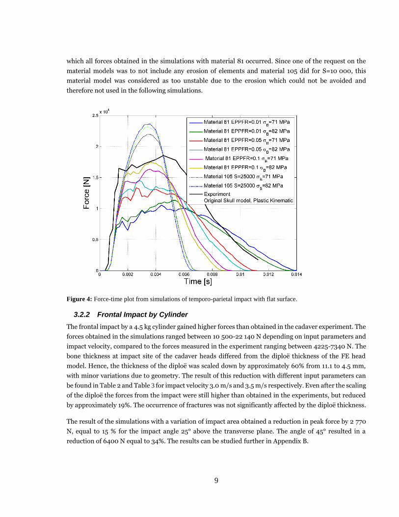
3.2.1 Temporo-Parietal Impact by Flat Surface
The forces obtained from the simulations of the temporo-parietal impact by flat surface are presented in
Figure 4. Material 105 with input parameter S=10 000 resulted in eroded elements at the impacted area,
on both inner and outer tables, independent of the σB used, hence are not a part of the presented results.
Input parameter S= 25 000 resulted in a stiff material for both σB, and the evolved damage was close to
zero. This can be seen by the absence of irregularities of the curve in the force-time plot. For all
simulations of material 81, no erosion was obtained and the force curve shows discontinuities around the
peak of the curve, indicating fracture [10], along with the trend of the curves following the experiment.
The peak forces obtained in the cadaver experiments ranged from 5 800-17 000 N, an interval within
9
which all forces obtained in the simulations with material 81 occurred. Since one of the request on the
material models was to not include any erosion of elements and material 105 did for S=10 000, this
material model was considered as too unstable due to the erosion which could not be avoided and
therefore not used in the following simulations.
Figure 4: Force-time plot from simulations of temporo-parietal impact with flat surface.
3.2.2 Frontal Impact by Cylinder
The frontal impact by a 4.5 kg cylinder gained higher forces than obtained in the cadaver experiment. The
forces obtained in the simulations ranged between 10 500-22 140 N depending on input parameters and
impact velocity, compared to the forces measured in the experiment ranging between 4225-7340 N. The
bone thickness at impact site of the cadaver heads differed from the diploë thickness of the FE head
model. Hence, the thickness of the diploë was scaled down by approximately 60% from 11.1 to 4.5 mm,
with minor variations due to geometry. The result of this reduction with different input parameters can
be found in Table 2 and Table 3 for impact velocity 3.0 m/s and 3.5 m/s respectively. Even after the scaling
of the diploë the forces from the impact were still higher than obtained in the experiments, but reduced
by approximately 19%. The occurrence of fractures was not significantly affected by the diploë thickness.
The result of the simulations with a variation of impact area obtained a reduction in peak force by 2 770
N, equal to 15 % for the impact angle 25° above the transverse plane. The angle of 45° resulted in a
reduction of 6400 N equal to 34%. The results can be studied further in Appendix B.

10
Table 2: Maximum force, fracture occurrence and force reduction due to diploë thickness reduction, at impact
velocity 3.0 m/s.
GEOMETRY σB [MPa] EPPFR MAX FORCE
[N]
FRACTURE REDUCTION
[%]
Original
diploë
71 0.01 14 540 Y
0.05 18 270 N
0.1 18 460 N
82 0.01 15 410 Y
0.05 18 710 N
0.1 19 040 N
Scaled diploë 71 0.01 11 220 Y 22.8
0.05 14 610 N 20.0
0.1 15 110 N 18.2
82 0.01 12 440 Y 19.3
0.05 15 520 N 17.1
0.1 15 730 N 17.4
Table 3: Maximum force, fracture occurrence and force reduction due to diploë thickness reduction, at impact
velocity 3.5 m/s.
GEOMETRY σB [MPa] EPPFR MAX FORCE
[N]
FRACTURE REDUCTION
[%]
Original
diploë
71 0.01 13 430 Y
0.05 18 140 Y
0.1 20 820 N
82 0.01 16 310 Y
0.05 20 860 N
0.1 22 140 N
Scaled diploë 71 0.01 10 500 Y 22.8
0.05 15 630 Y 14.9
0.1 16 970 N 18.5
82 0.01 12 170 Y 25.4
0.05 16 900 Y outer, N inner 19.0
0.1 17 980 N 18.8
3.2.3 Frontal Impact by Flat Surface
With the same input parameters and material model as in previous simulation, the simulations of the
frontal impact by a flat surface resulted in higher forces than obtained in the experiments. The diploë
thickness was reduced, equivalent to the experiment above. The results of the reduced diploë thickness

11
for all simulations can be found in Appendix B, along with the maximum forces and the fracture
occurrence. It was obtained that the reduction of the diploë resulted in a decreased maximum force of
2.96-14.00 % depending on impact velocity, EPPFR-value and σB. Since there was no information of the
impactor mass for the impact velocity 3.8 and 5.3 m/s available, the same mass as for the impact velocity
6.9 m/s was used. This assumption was made since the documentation from the experiments claimed
that the fractures occurred before any movement of the head, resulting in no impact from the moment of
inertia.
Impact velocity 3.8 m/s resulted in fractures for EPPFR=0.01 for both σB values and the two diploë
thicknesses. The force-time history can be found in Figure 5, showing irregularities of the curves for
EPPFR=0.01 but not for EPPFR=0.05 and 0.1. Since no fractures was obtained in the cadaver
experiment EPPFR=0.01 could here be considered to result in a too soft material.
Figure 5: Force-time plots from simulations of frontal impact by flat surface at impact velocity 3.8 m/s. The left
image shows the result from simulations with the original diploë and the right image shows the result from
simulations with the scaled diploë. Input variables EPPFR=0.01,0.05 and 0.1 were used for both σB=71 MPa and
82 MPa. No experimental force-time history was available to compare with.
The force-time curves from the simulations with impact velocity 5.3 m/s were compared to the force-time
curve available from the literature by Verscheuren et al. [12] and evaluated with regards to similarities of
the trends. Figure 6 shows the result from the simulations with impact velocity 5.3 m/s, different input
parameters and original and scaled diploë. It was obtained that the similarities of the trends of the curves
between the experiment and simulations were higher using the original diploë than with the scaled. As
seen in previous results, the scaled diploë resulted in lower peak forces, but for these simulations the
differences were minor.

12
Figure 6: Force-time plots from simulations of frontal impact by flat surface at impact velocity 5.3 m/s. The left
image shows the result from simulations with the original diploë and the right image shows the result from
simulations with the scaled diploë. Input variables EPPFR=0.01, 0.05 and 0.1 were used for both σB=71 MPa and
82 MPa. The black curve in both images is data extracted from the literature from the study by Verschueren et al.
[12].
Impact velocity 6.9 m/s resulted in fractures in all the experimental studies by Delye et al. [13] with
fracture forces ranging between 6 500-11 800 N. The simulations with this impact also resulted in
fractures with all input parameter variations, but with forces higher than those measured in the
experiments. The simulated forces were 2 900-14 040 N higher than the forces from the experiment,
depending on input parameters. The force-time curves of these simulations are found in Figure 7. The
simulations with the scaled diploë and EPPFR=0.01 resulted in negative volume elements, thus they were
excluded from the result.
The result from the impact site variation was obtained at simulations with impact velocity 6.9 m/s. An
increase of fracture force due to impact site could be obtained. The peak force increased by approximately
16 % for an impact site 9 mm superior to the impact site used in the other simulations. These results can
be found in Appendix B.

13
Figure 7: Force-time plots from simulations of frontal impact by flat surface at impact velocity 6.9 m/s. The left
image shows the result from simulations with the original diploë and the right image shows the result from
simulations with the scaled diploë. Input variables EPPFR=0.01,0.05 and 0.1 were used for both σB=71 MPa and
82 MPa, except from the scaled model where EPPFR=0.01 and both σB resulted in negative volume elements, hence
these results were eliminated.
3.2.4 Validation against Study of Vertex and Frontal Impact by Sphere
The result from the simulations of the vertex and frontal impact by sphere is found in the plot in Figure
8. By using material 81 and the input parameter EPPFR=0.05 these results were obtained. Fractures
occur for both impact sites and the different σB resulted in a minor difference in peak force but did not
impact the trend of the curves. The cadaver experiment showed peak forces of 13 600 N for frontal impact
and 8 800-14 000 N for the vertex impacts. Peak force for the frontal impact simulations was 13 530 N
and 14 250 N for σB=71 MPa and 82 MPa respectively. For the vertex impact the peak forces obtained in
the simulations were 11 520 N for σB=71 MPa and 12 350 N for σB=82 MPa.

14
Figure 8: Force-time plots with input parameter EPPFR=0.05. Frontal impact is presented in the image to the left
while the vertex impact is presented in the image to the right. The horizontal lines represent the maximum force
obtained in the experiments. The two lines in the right image shows the highest and lowest experimental value.
3.3 Fracture Prediction
The fracture prediction is based on the damage parameter. This parameter can be visualized by plotting
its propagation over the skull bone. The results of the damage propagation from the different simulations
are found in the sub-sections below. The red area shows the elements where the damage parameter
reached 1, indicating a failed element and thereby a fractured bone. By comparing the plotted damage
parameter with the documented fractures from the cadaver experiment, the fracture prediction can be
validated.
The material model 81 and EPPFR=0.05 was used when plotting the damage propagation to visualize the
fractures. According to the results presented above, using the EPPFR=0.01 resulted in a too soft material
in both temporo-parietal impact and frontal impact by flat surface. While using the EPPFR=0.1 resulted
in a too stiff material giving the highest peak forces in the simulations of the two different frontal impacts.
Hence, of the three EPPFR-values evaluated 0.05 was the most stable and accurate value and therefore
used to visualize the fractures.
3.3.1 Temporo-Parietal Impact by Flat Surface
The propagation of damage can be obtained from the plotted damage parameter and is presented in
Figure 9. A clear fracture can be obtained, due to the red area at the impact site. The reduction of the load
carrying capacity can be obtained from the decreased stresses as the damage evolved. It can be obtained
that as the stress decreases in one area the load is distributed to the surrounding elements. No
documentation of the injuries was available in the literature from the study by Allsop et.al. [10], hence no
further evaluation was possible for this result.

15
Figure 9: Plotted damage propagation and von Mises stress from simulation of the temporo-parietal impact, with
material 81 and input parameter EPPFR=0.05 and σB=82 MPa. The left column shows the result at the time where
the failure starts, middle column shows the result at the time for the maximum force, right column shows the result
at the end of the impact, where the impactor is no longer in contact with the head.
3.3.2 Frontal Impact by Cylinder
The forces obtained in the simulations of the frontal impact by cylinder were higher than those obtained
in the cadaver experiments, and fractures only occurred at the simulations using the input parameter
EPPFR=0.01. This, along with only 4/7 of the impacted cadaver head resulted in fractures made the
impact velocity 3.0 m/s an uncertain loading conditions to draw conclusions from. Instead the
simulations with the impact velocity 3.5 m/s were used to evaluate the fractures simulated. Figure 10
shows the damage and the von Mises stress from the simulation with the input parameters EPPFR=0.05
and σB=71 MPa.

16
Figure 10: Plotted damage propagation and von Mises stress from simulation of the frontal impact by cylinder,
with material 81 and input parameter EPPFR=0.05 and σB=71 MPa. The left column shows the result at the time for
initial contact, middle column shows the result at the time for the maximum force, right column shows the result at
the end of the impact, where the impactor is no longer in contact with the head.
3.3.3 Frontal Impact by Flat Surface
The cadaver experiments with the impact velocity 3.8 m/s did not result in any fractures and are therefore
not of interest in this section. The impact velocity 5.3 m/s resulted in fractures but no further
documentation of these results was available in the literature by Verschueren et al. [12]. Instead the
impact velocity 6.9 m/s was of higher interest to investigate as the documentation of the fracture was
available in [13]. The experiment resulted in complex fracture pattern at the impact site including a linear
fracture line towards the orbital rim. It was not possible to model the fracture propagation or draw
conclusions regarding type of fracture. However, the region for the damaged elements in the simulation,
see Figure 11, is similar to what was obtained in the cadaver experiments.

17
Figure 11: Plotted damage propagation and von Mises stress from simulation of the frontal impact by flat surface,
with material 81 and input parameter EPPFR=0.05 and σB=82 MPa. The left column shows the result at the time of
the initial impact, middle column shows the result at the time for the maximum force, right column shows the result
at the end of the impact, where the impactor is no longer in contact with the head.
3.3.4 Validation against Study of Vertex and Frontal Impact by Sphere
The last experiment was used as validation of the decided parameters, to investigate whether the most
accurate setup from the previous simulations would result in accurate fractures for other impacts. The
result from the impact of the vertex can be found in Figure 12. The fractures found in the cadaver
experiment are mainly described as multiple and circular at the vertex region. The fracture obtained from
the simulations of the frontal impact is found in Figure 13. The fracture obtained in the experiment was
described as multiple fractures at the frontal bone. In neither of the simulations could fracture pattern or
type of fracture be obtained, but the fractured region is similar in the cadaver experiment to the regions
of the model with ruptured elements from the simulations.

18
Figure 12: Plotted damage parameter over vertex region from simulation of vertex impact by sphere. The left image
shows the outer table while the right image represents the inner table.
Figure 13: Plotted damage parameter over the frontal bone, from simulation of frontal impact by sphere. The left
image shows the outer table while the right image represents the inner table.

19
4. Discussion
It was obtained that using the material model 81 with the input parameter EPPFR=0.05 gave the most
accurate results. Overall, when comparing the accuracy of the different results, it was obtained that the
EPPFR=0.01 resulted in a too soft material in the simulations of the frontal impact with flat surface and
temporo-parietal impact. It also resulted in negative volume elements when scaling the diploë at frontal
impact with flat surface and impact velocity 6.9 m/s. Hence, EPPFR=0.01 was considered as unstable
and not accurate enough. Simulations with EPPFR=0.1 resulted in a too stiff material, showed by the
highest peak forces in all frontal impact simulations. EPPFR=0.05 on the other hand, resulted in the most
accurate fracture prediction in all simulations as well as the most similar force-time plot trends, and was
therefore determined to be the most appropriate value for the input parameter EPPFR.
The coarse mesh of the skull bone in the head model was a major limitation. Since the elements are
relatively large the stress and strain concentrations are spread over a larger surface and therefore the
material fails, either in larger areas than in the cadaver experiments, or not at all. An explanation to the
higher forces could be the mesh size since the simulations of the impacts at the areas with denser mesh,
i.e. vertex and temporo-parietal, resulted in forces closer to those obtained in the cadaver experiments
than the impact at areas with coarser mesh, i.e. frontal. By comparing the results from the impacts by the
sphere it could be obtained that the forces at the vertex impact were lower than at the frontal impact. This
could be explained by the denser mesh at the vertex, but also by the thinner diploë at the vertex compared
to at the frontal impact site.
Mao et al. [16] performed simulations of the same cadaver experiment of frontal impact by cylinder and
did also obtained forces higher than the experimental. They obtained 23-123% higher forces depending
on the impact velocity, as well as no fractures at the lowest velocity 2.7 m/s. The FE head model used by
Mao et al. was the WSU FE head model described in Appendix A.5.2.1. It consisted of 270 500 elements,
compared to the 24 000 element of the KTH FE head model. The reason for both the study by Mao et al.
and the study performed during this project obtaining similar results might be due to some measurement-
errors during the experimental study or due to the dyelite padding used in the experiment which was not
modeled in the simulations. The Young’s modulus of the tables in the WSU FE head model was lower, 10
GPa, compared to the Young’s modulus of the model in this study, 17 GPa. The WSU FE head model was
also validated against the same cadaver experiment by Yoganandan as presented earlier in this report,
with results similar to the results from this study. The similarities in these results show that the mesh
density might affect the stiffness of the material, since a softer material with smaller mesh gave similar
results as a stiffer material with coarser mesh.
The FE head model used to develop the strain-based fracture criterion presented in Appendix A.5.3.3
used an elastic material model to model the skull with no plasticity, failure or damaged criterion included.
Instead the fracture prediction was based on the obtained strain levels from the FE simulations
correlating to the accelerations and forces at fracture obtained from cadaver and dummy experiments
[4], [18]. Modeling the skull bone with an elastic material model does not allow any reduction of the
strength of the bone due to yield or failure of the bone tissue, which could reduce the reliability of the
method. By using a material model enabling reduction of the strength of the material, such as the material

20
model used in this study or the material model of the SUFEHM [19] presented in Appendix A.5.2.2, the
behavior of the simulated material is more similar to the behavior of bone tissue.
The simulations of the temporo-parietal impact were mainly used to decide which material model to
continue with in further simulations. The requirements on the material model stated that no erosion of
elements was allowed and at the same time the load carrying ability should drop relatively fast. These
requests were obtained to be fulfilled when using material 81, but not with material 105. Since the cadaver
experiment of this impact included forces high enough to guarantee fractures and no fracture
documentation was available the possibility for further conclusions from this experiment were limited.
Another important aspect of these results is the source of error due to the limited amount of experimental
data and the large variation in results, geometries and material properties of the cadavers. The frontal
impact by sphere had one experimental result to compare to the result from the simulation. The
experimental results of the temporo-parietal impact showed a wide range of fracture forces, resulting in
a large interval within which the simulation results could be considered as reasonable. These
circumstances have to be taken into consideration when evaluating the accuracy of the results from this
kind of study, since they add uncertainties to the accuracy of the results obtained.
Assumptions were made regarding the impact site in the simulations of frontal impact by cylinder and
flat surface. The information in the literature was vague in both cases and therefore assumptions were
made following the descriptions as far as possible. Different impact sites were tested and evaluated, see
Appendix B, where it was obtained that the impact site has an effect on the result. In the simulations of
the frontal impact by cylinder the force was reduced the closer to the vertex the impactor hit the skull, but
compared to the results obtained from the cadaver experiments the forces were still significantly higher.
Different impact sites at the simulations of the frontal impact by sphere did not have any significant
impact on the result.
The investigation of the diploë thickness resulted in a reduced fracture force with a thinner diploë, but in
no or a minor increase of the fracture extent. This shows that the thickness of the diploë does not
significantly affect the occurrence of fractures. The initial assumption that the tables are more significant
for fracture prediction was thereby most likely correct.
The material models tested and used in this study did not enable any scaling of the material parameters
for different strain rates. The only scaling possible was for the plastic region of the stress-strain curve.
This curve obtained in the experiment by Wood et al. [9] showed that the strain rate affects the stress-
strain curve even in the elastic region, hence no strain rate variation could be accounted for. This is a
limitation that might have had an impact on the results, since the Young’s modulus, calculated from the
stress-strain curve, affects how the material behaves. For lower strain rates the material should have been
softer than the material developed in this study, and for higher strain rates it should have been stiffer.
To complete this model and to increase the reliability and exactness of the fracture prediction would
require some future work. One adjustment of the model could be to divide the skull bone into parts, for
example frontal, occipital, parietal, temporal and facial. This would enable different geometries and

21
material properties for the different skull bone parts. Another aspect, not only applicable for this study is
the scaling. With a method for scaling the whole model the simulations could be adjusted to mimic each
experimental setup, with the variations of cadaver geometry and mass. The fracture propagation would
also be interesting to study, but will demand a finer mesh, and a larger focus on the fracture mechanism
of bone tissue. The material model properties set for the diploë could also need a further investigation.
Young’s modulus of diploë might have an impact on the simulation results, It was in the current model
set to 1 GPa, but experiments have shown a large variation from 0.39-2.75 GPa [20]. The impact from
material mode of the diploë including damage or failure could also be relevant to evaluate. Lastly, a
further investigation of the impact on the inner parts of the FE head model due to this new skull bone
model would be interesting to perform, in order to determine its influence on the soft tissue responses.
As could be seen in the plot presenting the result from the temporo-parietal impact the force was reduced
by approximately 43% using the new material model for the skull bone compared to the old.

22
5. Conclusions
Following conclusions could be obtained from this project:
Material model 81 with input parameter EPPFR=0.05 gave the most stable simulations and
accurate results, both for fracture forces and fracture prediction.
The fracture prediction is limited, in terms of fracture propagation and type of fractures, due to
the coarse mesh of the model.
The breaking stress does not significantly affect the fracture modeling, but have an impact on the
peak forces obtained in all simulations.
The thickness of the diploë does not significantly affect the fracture modeling, but have an impact
on the peak forces obtained in the simulations of the frontal impacts.

23
References [1] E. Ehrlich, A. Tischer, and H. Maxeiner, “Lethal pedestrian - Passenger car collisions in Berlin.
Changed injury patterns in two different time intervals,” Leg. Med., vol. 11, no. SUPPL. 1, pp. S324–S326, 2009.
[2] G. Zhang, L. Cao, J. Hu, and K. H. Yang, “A field data analysis of risk factors affecting the injury risks in vehicle-to-pedestrian crashes.,” 52nd AAAM Annu. Conf. Ann. Adv. Automot. Med., vol. 52, no. October, pp. 199–214, 2008.
[3] Autoliv, “Pedestrian Protection.” [Online]. Available: https://www.autoliv.com/ProductsAndInnovations/PassiveSafetySystems/Pages/PedestrianProtection.aspx. [Accessed: 10-Dec-2015].
[4] M. Vander Vorst, P. Chan, J. Zhang, N. Yoganandan, and F. Pintar, “A new biomechanically-based criterion for lateral skull fracture.,” Annu. Proc. Assoc. Adv. Automot. Med., vol. 48, pp. 181–95, 2004.
[5] M. Fahlstedt, K. Baeck, P. Halldin, J. Vander Sloten, J. Goffin, B. Deprietere, and S. Kleiven, “Influence of Impact Velocity and Angle in a Detailed Reconstruction of a Bicycle Accident,” IRCOBI Conf., pp. 787–799, 2012.
[6] “LS-DYNA®.” Livermore Software Technology Corporation.
[7] “LS PrePost.” Livermore Software Technology Corporation.
[8] The MathWorks Inc., “MATLAB.” Natick, Massachusetts, United States, 2015.
[9] J. Wood, “Dynamic response of human cranial bone,” J. Biomech., vol. 4, no. 3, pp. 1–12, 1971.
[10] D. Allsop, T. Perl, and C. Warner, “Force/Deflection and Fracture Characteristics of the Temporo-parietal Region of the Human Head, Proceedings of 35th Stapp Car Crash Conference,” 1991, pp. 269–278.
[11] V. R. Hodgson, J. Brinn, L. M. Thomas, and S. W. Greenberg, “Fracture Behavior of the Skull Frontal Bone Against Cylindrical Surfaces,” Proceedings of Fourteenth Stapp Car Crash Conference. pp. 341–355, 1970.
[12] P. Verschueren, H. Delye, B. Depreitere, C. Van Lierde, B. Haex, D. Berckmans, I. Verpoest, J. Goffin, J. Vander Sloten, and G. Van der Perre, “A new test set-up for skull fracture characterisation,” J. Biomech., vol. 40, no. 15, pp. 3389–3396, 2007.
[13] H. Delye, P. Verschueren, B. Depreitere, I. Verpoest, D. Berckmans, J. Vander Sloten, G. Van Der Perre, J. Goffin, and J. O. S. Vander Sloten, “Biomechanics of frontal skull fracture.,” J. Neurotrauma, vol. 24, no. 10, pp. 1576–86, 2007.
[14] N. Yoganandan, F. A. Pintar, A. J. Sances, P. R. Walsh, C. L. Ewing, D. J. Thomas, and R. G. Snyder, “Biomechanics of Skull Fracture,” J. Neurotrauma, vol. 12, no. 4, pp. 659–668, 1995.
[15] M. Iwamoto and Y. Nakahira, “Development and Validation of the Total HUman Model for Safety (THUMS Version 5 Containing Multiple 1D Muscles for Estimating Occupant Motions with Muscle Activation During Side Impacts,” Stapp Car Crash J., vol. 59, no. 2012, pp. 53–90, 2015.
24
[16] H. Mao, L. Zhang, B. Jiang, V. V. Genthikatti, X. Jin, F. Zhu, R. Makwana, A. Gill, G. Jandir, A. Singh, and K. H. Yang, “Development of a Finite Element Human Head Model Partially Validated With Thirty Five Experimental Cases,” J. Biomech. Eng., vol. 135, no. 11, pp. 1–15, 2013.
[17] Z. Asgharpour, D. Baumgartner, R. Willinger, M. Graw, and S. Peldschus, “The validation and application of a finite element human head model for frontal skull fracture analysis,” J. Mech. Behav. Biomed. Mater., vol. 33, no. 1, pp. 16–23, 2014.
[18] P. Chan, Z. Lu, P. Rigby, E. Takhunts, J. Zhang, N. Yoganandan, and F. Pintar, “Development of a Generalized Linear Skull Fracture Criterion,” National Highway Traffic Safety Administration, US Department of Transportation, 07-0227, 2007.
[19] D. Sahoo, C. Deck, N. Yoganandan, and R. Willinger, “Anisotropic composite human skull model and skull fracture validation against temporo-parietal skull fracture,” J. Mech. Behav. Biomed. Mater., vol. 28, pp. 340–353, 2013.
[20] J. W. Melvin, D. H. Robbins, and V. . Roberts, “The Mechanical Behaviour of the Diploë Layer of the Human Skull in Compression,” Dev. Mech., vol. 5, pp. 811–816, 1969.


APPENDIX


APPENDIX A
Background and literature study.
Table of Contents
1 Introduction .............................................................................................................. I
1.1 Injury Profiles ......................................................................................................................I
1.2 Anatomy ...............................................................................................................................I
2 Cranial Bone Properties ...................................................................................... IV
2.1 Experimental studies on cranial bone properties ......................................................... IV
2.2 Fractures of Cranial Bone ............................................................................................... VI
3 Modeling and Experimental Methods of Tolerance Investigation ............. VII
3.1 Anthropomorphic Test Device ....................................................................................... VII
3.2 Post Mortem Human Surrogates ................................................................................... VII
3.3 Mathematical model ........................................................................................................ VII
4 Finite Element Method................................................................................. VIII
4.1 FE Analysis ..................................................................................................................... VIII
4.2 FE Modeling .................................................................................................................... VIII
4.3 Material models .............................................................................................................. VIII
5 Skull Fracture Studies .................................................................................... X
5.1 Cadaver experiments ........................................................................................................ X
5.2 Head models .................................................................................................................... XII
5.2.1 Wayne State University (WSU) ........................................................................ XII
5.2.2 Strasbourg University Finite Element Head Model (SUFEHM) ............................. XII
5.2.3 THUMS-KTH model ....................................................................................... XII
5.3 Skull fracture criteria ..................................................................................................... XIII
5.3.1 Linear acceleration ........................................................................................ XIII
5.3.2 Stress .......................................................................................................... XIII
5.3.3 Strain .......................................................................................................... XIV
5.3.4 Energy......................................................................................................... XIV
References ................................................................................................................... XV


I
1 Introduction
The aim of this master thesis is to develop a method for probabilistic skull fracture prediction, suitable
for pedestrian-vehicle accident applications. In this background chapter, the essentials of anatomy,
bone properties and finite element (FE) analysis are presented, followed by recent studies within this
area and different FE head models.
This first section of the background chapter serves as a brief introduction. It contains the basic
kinematics of pedestrian accidents and a brief explanation of the anatomy of the skull.
1.1 Injury Profiles
In pedestrian-vehicle crashes, the pedestrian is very fragile and unprotected compared to the driver
of the car. In Europe, almost 30 % of the non-fatal road accidents involving pedestrians between 2005
and 2008 led to head injuries [1].
The kinematics of a pedestrian being hit by the front of a car can be divided into, in chronological
order, the primary impact, followed by a flight phase which results in a ground impact and lastly a
sliding phase [2]. Depending on the properties of the pedestrian, i.e. height and mass, the shape of
the hood and the impacting velocity the number of impacts will differ and thereby also the injuries
[2]. A study of accident reconstructions, where a 50th percentile male being hit by a sports car at a
velocity of 40 km/h, shows that after the primary impact to the lower extremities the head will be
impacted by the windshield or the bonnet in the middle of the flight phase before hitting the ground
[2]. The same study shows that the area functioning as the primary impactor might vary depending
on the accident parameters, e.g. impacting velocity and pedestrian parameters. This leads to the
conclusion that both the vehicle and the ground might serve as impactors to the head at pedestrian-
vehicle accidents.
1.2 Anatomy
The skull consists of two main areas; the cranium and the face. The cranium is the main protector of
the brain from external impacts. All the bones of the cranium are connected to each other by fixed
joints called sutures. The sutures are reinforced and surrounded by compact bone [3]. The cranium
consists of eight bones; the frontal, the left and right parietal, the left and right temporal, the occipital,
the sphenoid and the ethmoid bone [4]. The locations of these bones are illustrated in Figure 1.

II
Figure 1: Bones of the human skull [5].
The cranial bones consist of two thin layers of compact bone called the inner and outer table and a
core of cancellous bone called the diploë [6]. The main purposes of the diploë are to maintain the
shape of the cranial bone and to function as a resistance against shear stresses [7]. The thickness of
the diploë varies between people and regions of the cranial bone [6]. The thickness usually increases
closer to the center of the bone, and decreases closer to the sutures. This thickness variation can be
seen in Figure 2.
.
Figure 2: Image of sagittal cut through the cranial bone [5].
The grain structure of the compact bones in the tables is randomly organized, giving the cranial bones
a transversely isotropic mechanical behaviour [6]. The structure of the cranial bone is a sandwich

III
structure where the stiff layers are the inner and outer table, and the softer core is the diploë. The
thickness and the density of the diploë influence the mechanical behaviour of the cranial bone, e.g.
the failure strength and energy absorption [6], [8].

IV
2 Cranial Bone Properties
There have been several studies performed to determine the mechanical properties of cranial bone.
Young’s modulus (E), Poisson’s ratio (ν), bulk modulus (G), breaking stresses and strains (σB, εB) in
tension and compression are a few of the properties examined and the results from some of these
studies are presented below.
The characteristic sandwich structure of the cranial bone has special mechanical behaviours and
fracture mechanics. There are four ways in which a sandwich construction can deform; membrane
deformation, bending deformation, shear deformation and local core compression and puncture [9].
In the cranial bone a membrane deformation is a stretch or compression of the layered structure,
giving resultant forces of the same magnitude in the inner and outer tables. Bending deformations
result in tensile stresses in one of the tables and compressive stresses in the other. Shearing
deformation is primarily due to deformations of the diploë, because of its lower stiffness. This mainly
occurs from a transversely applied load. Compressive deformation of the structure is also due to the
lower stiffness of the diploë, enabling it to deform more easily than the tables [9].
2.1 Experimental studies on cranial bone properties
McElhaney et al. [6] made several experiments on specimens from embalmed human cadavers, with
an age range of 56 to 73 years at death, and craniotomies to obtain material properties of human
cranial bone. The experiments were performed on the frontal, occipital and left and right parietal
bone. The specimens were tested in compression, simple shear, torsion and strength. From these
experiments Young’s modulus, Poisson’s ratio and ultimate compression stresses and strains, all in
both radial and tangential directions were determined. Tension tests were also performed, but only
in the tangential direction. The directional variations showed that the Young’s modulus in tangential
compression was generally more than twice the modulus for radial compression. The ultimate
strength was also higher in tangential direction than in radial. Though, ultimate strain and energy
absorption were larger in compression in radial direction compared to the tangential direction. The
thickness of the diploë was determined for each specimen as well as its impact on the material
properties. It appeared that an increased diploë thickness resulted in a reduced radial compressive
modulus and ultimate strength, while the energy absorption was increased. Another finding from this
study was that the mechanical properties of compact bone are more uniform and predictable than
cancellous bone. In the cancellous bone there are marrow spaces of different sizes impacting the
mechanical properties. A summary of the mechanical properties obtained in this study can be found
in Table 1.

V
Table 1: Material properties of human cranial bone[6]. *indicates significant variation between skulls. Notation
1 indicates properties in the radial direction while notation 2 and 3 indicates properties in the tangential plane.
Notation C specifies a property obtained from compression tests, and T indicates a property in tension.
PROPERTY VALUE
ν12 0.19
ν23 0.22
Ec1 2.41 GPa
Ec2 5.58 GPa
σB,c1 73.77 Mpa*
σB,c2 96.55 MPa
σB,table,T 79.29 MPa
εB,c1 0.097
εB,c2 0.051
Etable,T 12.27 GPa
Melvin et al. [10] studied the mechanical behaviour of the diploë layer in compression. The specimens
were tested at strain rates varying from 0.22 s-1 to 2.20 s-1 and Young’s modulus were determined,
ranging from 0.39 to 2.78 GPa. No correlations between the mechanical behaviour and the varying
strain rates were obtained. Another study where the impact from varying strain rates was investigated
was performed by Wood et al. [8]. In difference from the study by Melvin et al., Wood et al.
investigated the material properties of the tables. The specimens were extracted from the left and
right temporal bone and the frontal bone from 30 subjects with an age range of 25-95 years. The
Young’s modulus, breaking stress, breaking strain and energy absorbed to failure were obtained at
strain rates varying from 0.01 to 100 sec-1. The main results from this study showed that the
properties of the cranial bone had no directional variations in the tangential plane, meaning it behaves
transversely isotropic. The modulus of elasticity, breaking strain and breaking stress turned out to be
strain rate dependent, while the energy absorption was not. It also showed that there was no
significant difference in the modulus based on age or side of body. The same study also determined
the stress-strain relationship at strain rates of 0.1, 10 and 150 s-1. The results from these tests are
presented in the plot in Figure 3.
Figure 3: Stress-strain curve for strain rates 0.1, 10 and 150 s-1 [8].

VI
2.2 Fractures of Cranial Bone
Bone in tension deforms rather little before fracturing, and the surface of the fracture is not very
smooth [7]. Therefore bone tissue can be modeled as a fibrous composite with continuous fibers. Bone
consists of a softer matrix of collagen and the stronger mineral phase of the bone consists of
hydroxyapatite [7]. The strength and Young’s modulus of the hydroxyapatite reinforced fibers are
higher than for collagen. When a load is applied the ultimate strain level of the fibers will therefore
be reached before the failure stress of the matrix [7].
The cranial bone has higher tensile strength and Young’s modulus in the tangential direction than in
the radial direction. This can be explained by the Voigt and Reuss model. If the load is applied parallel
to the layers the stiffnesses of the two layers are additive, called the Voigt model, and if the load is
applied normal to the layers the compliance (inverse of the stiffness) of the layers are additive, called
the Reuss model [7]. There are regional differences in the strength of the skull bone. In respect to
fractures the bone is strongest in the rear, followed by the side and front [11].
An impacting force results in an out bending of the bone in the area near the impact site. Since bone
is weaker in tension than in compression, this out bending will be the cause of a linear skull fracture
[12]. Hence the tensile properties are more relevant than the compressive for skull fracture prediction.
There are different types of skull fractures. A linear skull fracture is the most common fracture and is
characterized by a break in the bone but no displacement [13]. These fractures are usually caused by
a low energy transfer due to trauma over a larger surface. A linear fracture affects the entire thickness
of the skull bone. In difference to a linear skull fracture, a depressed skull fracture occurs when a bone
fragment is compressed deeper than the underlying inner table. These fractures are usually caused by
high energy transfer with a small impacting surface [13]. Other skull fracture types are diastatic skull
fractures where the fracture occurs along the sutures, and basilar skull fractures, a fracture at the base
of the skull [13].

VII
3 Modeling and Experimental Methods of Tolerance
Investigation
There are three main methods for biomechanical tolerance investigation: Anthropomorphic Test
Device (ATD) experiments, Post Mortem Human Subjects (PMHS) experiments and mathematical
models, e.g. FE analysis [14]. Each method is described briefly in the following sections.
3.1 Anthropomorphic Test Device
ATD, also called dummy is a mechanical analog with the aim to mimic the anthropometry and
structural response of a human body [15]. They have to mimic both the internal and external human
behaviour, and is therefore constructed of metal, foams and composite polymer [15]. The dummies
are also equipped with sensors to measure accelerations, forces and displacements, to investigate the
tolerances.
3.2 Post Mortem Human Surrogates
Using human cadavers, or PMHS, can provide deterministic data, due to the anatomical equivalency
to an in vivo human [14]. Mathematical simulations do not have the possibility to determine injury
tolerance, since no failure criterion is known for complex biological tissues. Instead the results from
the mathematical simulations have to be validated against experiments performed on PMHS [14].
The tests can be performed to mimic a real accident with high level of similarity. Issues related to
PMHS are the lack of muscle tension and the presence of rigor mortis, causing tissue rigidity [15].
3.3 Mathematical model
Mathematical modeling of human bodies can be done, mainly in three different ways: as lumped mass
models, rigid body models or as finite element models (FE models). FE models are the most
commonly used and most reliable of these three types [15], and is therefore the focus of the following
section.

VIII
4 Finite Element Method
The finite element method is a technique for solving partial differential equations. The method has
several applications [16] and is, in this study, used to predict deformations and stress fields of solid
bodies exposed to external forces.
4.1 FE Analysis
A solid body is approximated into a finite number of discrete elements, interconnected with discrete
points called nodes at the boundary of each element. The shape of the elements varies depending on
the geometry of the body and each element type has its own set of shape functions. As a solid body
deforms, each node moves to a new position. These movements are called nodal displacements and
are, together with the shape functions, the basis of the approximation of the solution to the partial
differential equations [16].
Usually the FE models are implemented and solved with a computer. The software used for the FE
analysis in this study is LS-DYNA [17]. It is a finite element code for analysing large deformation
dynamic responses of structures, where the solutions are mainly based on explicit time integration,
e.g. central difference method [18].
Boundary conditions and material properties have to be set before the calculations start. The
boundary conditions are specified as the loads applied to the body, e.g. constraints. The material
properties are set by specifying constitutive laws for the body. In the case of a dynamic problem, initial
conditions, e.g. initial velocity, have to be set as well [16].
4.2 FE Modeling
FE modeling is usually divided into three stages; pre-, main and post-processing. Development of
geometric models, meshing and determination of material properties, as well as boundary conditions
are called pre-processing. This is followed by the numerical solution using the finite element method,
which is the main processing, and finally the visualization and analytical interpretation of results
called the post-processing [19].
A geometry is usually constructed using a Computer Aided Design tool or based on medical images,
and then meshed using a mesh generator [20]. The method used to model the skull, i.e. the type of
element used and the material properties set, is affecting the results when investigating brain tissue
impact responses. It has been obtained that, with equal impacts, a cranium modeled with composite
elements representing the tables and diploë will result in an increased intracranial pressure and
decreased countercoup pressure, compared to modeling the cranium with the compact tables as shell
elements and the diploë as brick elements [21]. It will result in an increased countercoup pressure
and von Mises stress on the brain tissue and a reduction of intracranial pressure.
4.3 Material models
There are several damage models available in LS-DYNA, for different types of materials. Generally,
when damage occur the strength of the material is decreased by a damage parameter D, where 0 ≤ D
≤ 1 [22]. The different models use different methods for determination of the damage parameter and
can be based on tensile strains and rupture limits of the strain, volumetric damage due to tensile

IX
strains, or shear stresses. The appropriate type of damage model depends on the material properties
and the elements used in the model, as well as the desired output data.
The material model MAT_DAMAGE_2 is suitable for computations on shell elements [18]. The
damage factor is based on Continuum Damage Mechanics (CDM) [18]. The CDM model computes the
damage factor from the accumulated plastic strain in tension [23]. The damage variable is calculated
according to equation (1). The stress-strain relationship can be tabulated to mimic the behaviour of
the material simulated.
(1 )
YD r
S D
(1)
Here, D is the evolution of the damage parameter D, Y is the strain energy release rate, a function of
the Young’s modulus and Poisson’s ratio. S is a pre-set constant and r is calculated according to
equation (2) below,
(1 )p
effr D (2)
where p
eff is the accumulation of effective plastic strain.
MAT_PLASTICITY_WITH_DAMAGE is applicable for shell elements and can be used for
orthotropic materials. The damage parameter is derived from the effective plastic strain obtained in
the material, p
eff , and the pre-set values for plastic strain at initiated failure,
p
failure , and effective
plastic strain at which the material ruptures, p
rupture [24]. The damage parameter is calculated
following equation (3). Equal to MAT_DAMAGE_2 the stress-strain relationship can be tabulated to
mimic the behaviour of the material.
p p
eff failure
p p
rupture failure
D
(3)

X
5 Skull Fracture Studies
This section will present different studies performed to investigate skull fractures. The presented
studies include cadaver experiments, different FE head models with different material models and
constitutive relations as well as different types on fracture criteria.
5.1 Cadaver experiments
Several cadaver experiments with different impactors and constraints are available in the literature.
Hodgson et al. [25], performed a study where a cylinder, with radius 25.4 mm, impacted the frontal
area, symmetrical with respect to the sagittal plane. Other experiments with frontal impact were
performed by Delye et al. [26] and Verschueren et al. [27] including a double pendulum where the
head was attached to one of the pendulum and on the other pendulum the 70 mm radius, flat surfaced
aluminium impactor was placed. The frontal area of the heads was impacted with velocities of 3.8, 5.3
and 6.9 m/s. Yoganandan et al. [28], performed a study where the load was applied to the vertex and
the frontal bone by a hemispherical anvil with the radius of 48 mm, at a velocity of 7.1-8.0 m/s.
Another study was performed by Allsop et al. [29] where eleven cadaver heads, impacted at the
parietal region by a flat surfaced box with a surface area of 0.005 m2. A summary of these experiments,
including specimen specifications, setup, results and available injury documentation is presented in
Table 2.

XI
Table 2: Summary of cadaver experiments
EXPERIMENT HODGSON ET AL.
[25]
DELYE ET AL.
[26] and
VERSCHUEREN
ET AL. [27]
YOGANANDAN ET
AL. [28]
ALLSOP ET AL.
[29]
NUMBER OF
CADAVERS
5 Delye 3 (6.9 m/s)
Verschueren 3 (3.8
and 5.3 m/s)
1 frontal
4 vertex
11
BONE THICKNESS
[mm]
Outer table: 2.08
Diploë: 2.00
Inner table: 2.03
(average)
Average: 8.66
Max: 10.75
Min: 5.42
- -
SCALP THICKNESS
[mm]
Average: 3.94
Max: 5.33
Min: 2.03
Average: 3.15
Max: 4.64
Min: 1.51
Average: 7.00
Max: 10.00
Min: 5.00
-
HEAD MASS [kg] Average: 3.88
Max: 4.67
Min: 3.36
Average: 3.43
Max: 4.18
Min: 2.66
Average: 3.47
Max: 4.12
Min: 2.81
-
AGE RANGE [years] 59-79 62-90 50-78 19-90
IMPACTOR Cylinder
Radius:25.4 mm
Length: 165.10 mm
Mass: 4.46 kg
Flat surfaced
cylindrical surface
Radius: 35 mm.
Mass: 28.9 kg
Hemisphere
Radius: 48.00 mm
Rectangular plate:
50x100 mm
IMPACTED REGION Frontal, symmetrical
with respect to the
sagittal plane, at the
smallest radius of the
forehead.
Frontal 1 Frontal (45°)
4 Vertex
Parietal
CONSTRAINTS Head attached to body,
free to rebound after
impact.
Double pendulum. 1
DoF, allowing
movement in the
plane of impact.
Head mounted in
fixation device, allowing
0 DoF.
Head mounted in
gypsum, allowing
0 DoF.
IMPACTING
VELOCITY [m/s]
Average: 2.93
Max: 3.54
Min: 2.74
3.8, 5.3 and 6.90 7.10-8.00 4.30
RESULTS Fracture force:
3 110-7 695 N
3.8 m/s No fractures
5.3 m/s Fracture
force: 15 000 N
6.9 m/s Fracture
force:
6 450-11 800 N
Fracture force frontal:
13 600N
Fracture force vertex:
8 800-14 000 N
Fracture force:
5 800-17 000 N
Average: 12 390 N
INJURY
DOCUMENTATION
3/5 localized fractures
originating from
supraorbital notch,
elliptically shaped. Inner
table involved.
2/5 linear fracture
originating from
supraorbital notch.
5.3 m/s: 2/3 linear
fractures,
1/3 depressed
fracture.
6.9 m/s: 4/4 linear
fracture from impact
site to orbital rim,
including complex
fracture pattern at
impact site.
Frontal: Multiple
fractures of frontal bone.
Vertex: 1/4 linear
fracture from vertex to
right orbit.
1/4 circular fracture in
vertex region.
2/4 multiple fracture,
vertex frontal and
temporal bone.
Bilaterally, parietal
bone.
Impacted the
specimens with
enough load to
cause fracture. No
documentation of
the type of fracture
was available.

XII
5.2 Head models
There are several FE head models available. The variation of the models ranges from different head
sizes and masses to different modeling methods with varying choices of element types and sizes,
geometries and material models. The models presented below have all been used for studies on skull
fractures.
5.2.1 Wayne State University (WSU)
One of the more recent models was developed at Wayne State University consisting of scalp, skull
bones as well as the parts of the brain and brainstem, modeled by a total of 270 552 elements [30].
The skull is modeled by layers of hexahedral elements, where the inner and outer layers represented
the tables and the middle layer the diploë. The thickness of the tables was fairly consistent over the
geometry while there was a larger thickness variation of the diploë layer. This thickness variation was
based on a study performed by Lynnerup et al. [31]. The material used to model both tables and diploë
was an elastic-plastic material. Young’s modulus for the tables was defined as 10 GPa, based on the
studies by Wood et al. [8] and the diploë was modeled with a Young’s modulus of 0.6 GPa, which was
obtained by Melvin et al. [10]. No regional differences in modulus were modeled for the tables or
diploë. This model was validated against thirty five experimental cases with PMHS, which showed a
close approximation of peak forces and prediction of type of skull fracture [30].
5.2.2 Strasbourg University Finite Element Head Model (SUFEHM)
Sahoo et al. [32] presented a head model with a skull modeled as an anisotropic material, called
SUFEHM. The skull was modeled with shell elements representing the diploë and the tables with
thicknesses of 3 mm and 2 mm, respectively. The density of the tables was 1 900 kg/m3 and Young’s
modulus was 15 GPa. Poisson’s ratio was 0.21 and the compressive and tensile strength were 132 MPa
and 90 MPa, respectively. For the diploë the density was set to 1 500 kg/m3, Young’s modulus was
4.67 MPa and Poisson’s ratio was 0.05. Compressive and tensile strength was set to 24.8 MPa and
34.8 MPa, respectively. The material model from LS-DYNA used to model the skull was
MAT_ENHANCED_COMPOSITE_DAMAGE.
5.2.3 THUMS-KTH model
The skull of the THUMS-KTH model was modeled as two layers of shell elements, representing the
inner and outer tables, with an inner core of solid elements with varying thickness, representing the
diploë. The inner and outer tables were modeled with the material model
MAT_PLASTIC_KINEMATIC with a density of 2009.14 kg/m3, Young’s modulus of 15 GPa, Poisson’s
ratio of 0.22 and a yield stress of 80 MPa [33]. The elements of the tables were shell elements, with a
Belytschko-Tsay formulation, which is the most computer capacity saving type of shell element [34].
The inner and outer tables were modeled with constant thicknesses of 1.83 mm and 1.96 mm
respectively. The material set for the diploë was MAT_ISOTROPIC_ELASTIC_PLASTIC, with a
density of 1109.75 kg/m3, shear modulus of 420 MPa, yield stress at 32.70 MPa and bulk modulus of
537 MPa. The material has an isotropic plasticity model, meaning that the element has the same yield
properties in all directions. This material type needs less computer resources, but a drawback of it is
the inaccurate shell thickness updates after yielding.

XIII
5.3 Skull fracture criteria
There are several methods developed for probabilistic prediction of different types of head injuries
and skull fractures. A selection of these methods are presented in the following sections.
5.3.1 Linear acceleration
Vander Vorst et al. [35] developed a global criterion called Skull Fracture Correlate, SFC. It is a
criterion developed from the Head Injury Criterion, HIC [36], and therefore based on the linear
acceleration of the center of mass during impact time. Equation (4) below describes SFC.
2
1
2 1
( )d
SFC( )
t
ta t t
t t
(4)
Here, t2-t1 is the time which maximizes the integral, and a(t) is the resultant acceleration at the center
of gravity of the head, during the impact time. This gives the average acceleration during the impact
time and is expressed in gravitational acceleration, with the unit g. SFC gives a probability-based
index of how likely a skull fracture will occur due to the calculated average linear acceleration. This
criterion has been evaluated by Chan et al. [11] where both lateral and frontal impacts were
investigated, and both PMHS experiments as well as a FE model were used. In both studies
logarithmic regression curves were obtained from the results of the FE model simulations and the
PMHS experiments. Vander Vorst et al. [37] found a SFC for a probability of 15% to gain a skull
fracture was at 120 g with a confidence band of 73 g< SFC15% <149 g. Chan et al. [11] obtained a
generalized SFC value for both frontal and lateral impact at a probability of 15% to gain a skull fracture
at 124 g, with a confidence band of 96 g< SFC15% <144 g.
5.3.2 Stress
Katagiri et al. [38], developed a skull fracture criteria based on the relation between stress and the
impact duration time. This study was based on a comparison between PMHS experiments performed
by Yoganandan et al. [28] and a FE head model of a Japanese male. The FE model was constructed of
22345 elements, with scalp, skull and brain, with a total mass of 3.36 kg. The skull was modeled as
quadrangular shell elements with a 1.7 mm thickness of the inner and outer table. The diploë was
modeled with two layers of solid elements with a varying total thickness of 3-8 mm. This study
resulted in a critical tensile stress and a critical compressive stress expressed in equation (5) and (6)
respectively.
0.5225( ) 44.7
tension
critt t
(5)
0.5429( ) 163.8
compression
critt t
(6)
Here, σ is the critical tensile and compressive stresses, respectively, and Δtσ is their respective
duration time.

XIV
5.3.3 Strain
Fractures in the skull bone occur when the ultimate strain is exceeded [37]. Therefore the strain of
the bone tissue can also be used as criterion for probabilistic prediction of skull fractures. From a
failure point of view, tensile stresses are more important than compressive stresses [8].
Chan et al. [11] compared PMHS experiments with simulations of the same impact conditions on a
FE model, and obtained logarithmic regression curves of the strain measured in the FE simulation
and the probability of fracture obtained from the PMHS experiments. The FE model was composed
of 24 000 elements, including outer and inner tables, diploë, brain, scalp and face with a total mass
of 4.54 kg. The thickness of the inner and outer tables was set to 1.3 mm and had a Young’s modulus
of 16 GPa and Poisson’s ratio of 0.35. The diploë was set to be 3 mm thick, with a Young’s modulus of
0.73 GPa and Poisson’s ratio of 0.05. The probability, P, of a skull fracture for frontal and lateral
impacts was expressed as equation (7) and (8) respectively.
ln 6.51* ln( ) 9.211
Pstrain
P
(7)
ln 5.12* ln( ) 6.361
Pstrain
P
(8)
This study obtained 22% mean probability to gain a skull fracture from a frontal impact at 0.2% strain,
while the same strain resulted in 18% mean probability for a skull fracture from a lateral impact.
5.3.4 Energy
Willinger et al. [39], derived injury criteria based on the ULP head FE model which is a previous
version of the SUFEHM. The injury criterion obtained from this study was a 50% risk of skull fracture
at a local strain energy level of 2.2 J. By comparing 64 real world accidents with the same impact
applied to the ULP model this injury level could be obtained.
Sahoo et al. [32], performed a study on the SUFEHM model for temporo-parietal skull fractures and
validated the model against 15 experimental cases on PMHS. They obtained a strain energy level of
554 mJ for 50 % risk of skull fracture.

XV
References [1] European Road Safety Observatory, “Traffic Safety Basic Facts 2015 Pedestrians,” 2012.
[2] M. Hamacher, L. Eckstein, and R. Paas, “Vehicle related influence of post-car impact pedestrian kinematics on secondary impact,” Proc. 2012 Int. {IRCOBI} Conf. Biomech. Inj., vol. 12, pp. 717–729, 2012.
[3] S. Kleiven, “Finite Element Modeling of the Human Head,” Ph.D dissertation, Department of Aeronautics, Royal Institute of Technology, Stockholm, 2002.
[4] C. Hollins, Basic Guide to Anathomy and Physiology for Dental Care Professionals. West Sussex, UK: John Wiley & Sons, Ltd, 2012.
[5] C. Vandyke and H. Gray, Anatomy of the Human Body, 20th ed. Philadelphia, New York: Lea and Febiger, 1918.
[6] J. H. McElhaney, J. L. Fogle, J. W. Melvin, R. R. Haynes, V. L. Roberts, and N. M. Alem, “Mechanical properties of cranial bone,” J. Biomech., vol. 3, no. 5, pp. 495–496,IN5,497–511, 1970.
[7] J. Currey, The Mechanical Adaptations of Bones. Princeton, New Jersey: Princeton University Press, 1984.
[8] J. Wood, “Dynamic response of human cranial bone,” J. Biomech., vol. 4, no. 3, pp. 1–12, 1971.
[9] R. P. Hubbard, “Flexure of Layered Cranial Bone,” J. Biomech., vol. 4, pp. 251–263, 1971.
[10] J. W. Melvin, D. H. Robbins, and V. . Roberts, “The Mechanical Behaviour of the Diploë Layer of the Human Skull in Compression,” Dev. Mech., vol. 5, pp. 811–816, 1969.
[11] P. Chan, Z. Lu, P. Rigby, E. Takhunts, J. Zhang, N. Yoganandan, and F. Pintar, “Development of a Generalized Linear Skull Fracture Criterion,” National Highway Traffic Safety Administration, US Department of Transportation, 07-0227, 2007.
[12] E. S. Gurdjan, H. R. Lissner, and J. E. Webster, “The Mechanism of Production of Linear Skull Fracture,” Surgery, Gynecol. Obstet., vol. 85, pp. 195–210, 1947.
[13] A. Nawaz Khan, S. Macdonald, I. Turnbull, R. Al-Okaili, and D. C. Phillips, “Imaging in Skull Fractures,” Medscape, Drugs & Diseases, 2015. [Online]. Available: http://emedicine.medscape.com/article/343764-overview. [Accessed: 12-Apr-2016].
[14] N. Yoganandan and F. A. Pintar, “Biomechanics of temporo-parietal skull fracture,” Clin. Biomech., vol. 19, no. 3, pp. 225–239, 2004.
[15] J. R. Crandall, D. Bose, J. Forman, C. D. Untaroiu, C. Arregui-Dalmases, C. G. Shaw, and J. R. Kerrigan, “Human surrogates for injury biomechanics research,” Clin. Anat., vol. 24, no. 3, pp. 362–371, 2011.
[16] A. F. Bower, Applied Mechanics of Solids. Taylor and Francis, 2012.
[17] “LS-DYNA®.” Livermore Software Technology Corporation.
[18] J. O. Hallquist, LS-DYNA Theoretical Manual, vol. 12. Livermore, California: Livermore Software Technology Corporation, 1998.
[19] Y. M. Desai, T. I. Eldho, and A. H. Shah, Finite Element Method with Applications in Engineering. Dorling Kindersley, India: Pearson Delhi, 2011.
[20] G. Krabbel and H. Appel, “Development of a finite element model of the human skull.,” J.

XVI
Neurotrauma, vol. 12, no. 4, pp. 735–742, 1995.
[21] T. J. Horgan and M. D. Gilchrist, “The creation of three-dimensional finite element models for simulating head impact biomechanics,” Int. J. Crashworthiness, vol. 8, no. 4, pp. 353–366, 2003.
[22] D. P. Nicolella and T. L. Bredbenner, “Computational Analysis of Bone Fracture,” in Accidental Injury, Biomechanics and Prevention, New York: Springer Science+Business Media, 2015, pp. 183–200.
[23] O. Lademo, O. S. Hopperstad, T. Berstad, and M. Langseth, “Numerical Simulations of Ductile Failure in Extruded Aluminium Alloys Using a Coupled Model of Elasto-Plasticity and Damage,” p. 9.
[24] Livermore Software Technology Corporation, LS-DYNA Keyword User’s Manual, vol. I, vol. I, no. May. 2007.
[25] V. R. Hodgson, J. Brinn, L. M. Thomas, and S. W. Greenberg, “Fracture Behavior of the Skull Frontal Bone Against Cylindrical Surfaces,” Proceedings of Fourteenth Stapp Car Crash Conference. pp. 341–355, 1970.
[26] H. Delye, P. Verschueren, B. Depreitere, I. Verpoest, D. Berckmans, J. Vander Sloten, G. Van Der Perre, J. Goffin, and J. O. S. Vander Sloten, “Biomechanics of frontal skull fracture.,” J. Neurotrauma, vol. 24, no. 10, pp. 1576–86, 2007.
[27] P. Verschueren, H. Delye, B. Depreitere, C. Van Lierde, B. Haex, D. Berckmans, I. Verpoest, J. Goffin, J. Vander Sloten, and G. Van der Perre, “A new test set-up for skull fracture characterisation,” J. Biomech., vol. 40, no. 15, pp. 3389–3396, 2007.
[28] N. Yoganandan, F. A. Pintar, A. J. Sances, P. R. Walsh, C. L. Ewing, D. J. Thomas, and R. G. Snyder, “Biomechanics of Skull Fracture,” J. Neurotrauma, vol. 12, no. 4, pp. 659–668, 1995.
[29] D. Allsop, T. Perl, and C. Warner, “Force/Deflection and Fracture Characteristics of the Temporo-parietal Region of the Human Head, Proceedings of 35th Stapp Car Crash Conference,” 1991, pp. 269–278.
[30] H. Mao, L. Zhang, B. Jiang, V. V. Genthikatti, X. Jin, F. Zhu, R. Makwana, A. Gill, G. Jandir, A. Singh, and K. H. Yang, “Development of a Finite Element Human Head Model Partially Validated With Thirty Five Experimental Cases,” J. Biomech. Eng., vol. 135, no. 11, pp. 1–15, 2013.
[31] N. Lynnerup, J. G. Astrup, and B. Sejrsen, “Thickness of the human cranial diploe in relation to age, sex and general body build.,” Head Face Med., vol. 1, p. 13, 2005.
[32] D. Sahoo, C. Deck, N. Yoganandan, and R. Willinger, “Anisotropic composite human skull model and skull fracture validation against temporo-parietal skull fracture,” J. Mech. Behav. Biomed. Mater., vol. 28, pp. 340–353, 2013.
[33] M. Fahlstedt, K. Baeck, P. Halldin, J. Vander Sloten, J. Goffin, B. Deprietere, and S. Kleiven, “Influence of Impact Velocity and Angle in a Detailed Reconstruction of a Bicycle Accident,” IRCOBI Conf., pp. 787–799, 2012.
[34] LSTC Inc and DYNAmore GmbH, “LS-DYNA support, Elements.” [Online]. Available: http://www.dynasupport.com/tutorial/ls-dyna-users-guide/elements. [Accessed: 23-Feb-2016].
[35] M. Vander Vorst, J. Stuhmiller, K. Ho, N. Yoganandan, and F. Pintar, “Statistically and biomechanically based criterion for impact-induced skull fracture.,” Annu. Proc. Assoc. Adv.

XVII
Automot. Med., vol. 47, pp. 363–81, 2003.
[36] Department of Transportation, Occupant Crash Protection-Head Injury Criterion S6.2 of MVSS 571.208, Docket 69-. Washington DC: NTHSA, 1972.
[37] M. Vander Vorst, P. Chan, J. Zhang, N. Yoganandan, and F. Pintar, “A new biomechanically-based criterion for lateral skull fracture.,” Annu. Proc. Assoc. Adv. Automot. Med., vol. 48, pp. 181–95, 2004.
[38] M. Katagiri, K. Katagata, J. A. Pramudita, and S. Ujihashi, “Development and application of stress-based skull fracture criteria using a head finite element model,” J. Biomech. Sci. Eng., vol. 7, no. 4, pp. 449–462, 2012.
[39] R. Willinger and D. Baumgartner, “Human head tolerance limits to specific injury mechanisms,” Int. J. Crashworthiness, vol. 8, no. 6, pp. 605–617, 2003.

XVIII

XIX
APPENDIX B
Results from the simulations of frontal impact by cylinder
Force-time plots for impact velocity 3.0 m/s and 3.5 m/s with original and scaled diploë.
Figure B.1: Force-time plot for the frontal impact by cylinder, with an impact velocity of 3.0 m/s. Material model
81 was used for the compact bone layers, with the input variable EPPFR and σB varied, and the model contained
the original thickness of the diploë.
Figure B.2: Force-time plot for the frontal impact by cylinder, with an impact velocity of 3.5 m/s. Material model 81
was used for the compact bone layers, with the input variable EPPFR and σB varied, and the model contained the
original thickness of the diploë.

XX
Figure B.3: Force-time plot for the frontal impact by cylinder, with an impact velocity of 3.0 m/s. Material model
81 was used for the compact bone layers, with the input variable EPPFR and σB varied, and the model contained
the scaled thickness of the diploë.
Figure B.4: Force-time plot for the frontal impact by cylinder, with an impact velocity of 3.0 m/s. Material model
81 was used for the compact bone layers, with the input variable EPPFR and σB varied, and the model contained
the scaled thickness of the diploë.

XXI
Force-time plots for impact velocity 3.5 m/s with a variation of impact sites.
Figure B.5: Result from the varied impact site of simulations of frontal impact by cylinder. The plots represents
the results from the impact site at an 0, 25 and 45 angle between inferior end of the diploë, the middle node of the
head and the middle of the impactor. The material model was material 81, with input parameter EPPFR=0.05 and
σB=71 MPa.

XXII
Results from the simulations of frontal impact by flat surface
Maximum force, fracture occurrence and force reduction due to decreased diploë thickness from
simulations of frontal impact by flat surface.
Table B.1: Maximum force, fracture occurrence and reduction of maximum force due to scaled diploë at impact
velocity 3.8 m/s.
GEOMETRY σB [MPa] EPPFR MAX FORCE
[N]
FRACTURE REDUCTION
[%]
Original diploë 71 0.01 14 620 Y
0.05 19 490 N
0.1 21 140 N
82 0.01 15 890 Y
0.05 21 370 N
0.1 21 870 N
Scaled diploë 71 0.01 13 530 Y 7.46
0.05 17 830 N 8.52
0.1 18 180 N 14.00
82 0.01 14 630 Y 7.93
0.05 18 670 N 12.63
0.1 18 820 N 13.95
Table B.2: Maximum force, fracture occurrence and reduction of maximum force due to scaled diploë at impact
velocity 5.3 m/s. Din and Dout are indicating that the failure level of the most damaged element which are not yet
failed, but showing where on the damage variable interval 0-1 the failure is.
GEOMETRY σB [MPa] EPPFR MAX FORCE
[N]
FRACTURE REDUCTION
[%]
Original diploë 71 0.01 13 670 Y
0.05 20 210 Y
0.1 21 720 Din=Y, Dout=0.38
82 0.01 15 980 Y
0.05 22 110 Y
0.1 25 310 Din=0.75, Dout=0.35
Scaled diploë 71 0.01 13 130 Y 3.95
0.05 18 840 Y 6.78
0.1 21 740 Din=Y, Dout=0.41 -0.09
82 0.01 14 140 Y 11.51
0.05 21 290 Y 3.71
0.1 23 570 Din=0.58, Dout=0.19 6.78

XXIII
Table B.3: Maximum force, fracture occurrence and reduction of maximum force due to scaled diploë at impact
velocity 6.9 m/s.
GEOMETRY σB [MPa] EPPFR MAX FORCE
[N]
FRACTURE REDUCTION
[%]
Original diploë 71 0.01 14 710 Y
0.05 20250 Y
0.1 22 990 Y
82 0.01 15 120 Y
0.05 22 050 Y
0.1 25 840 Y
Scaled diploë 71 0.01 - No result -
0.05 19 650 Y 2.96
0.1 21 180 Y 7.87
82 0.01 - No result -
0.05 20 290 Y 7.98
0.1 24 660 Y 4.57

XXIV
Result from impactor height variations for frontal impact by flat cylinder surface at an impact
velocity of 6.9 m/s.
Figure B.6: Results from the varied impact site for simulations of frontal impact by flat surface at impact velocity
6.9 m/s. The plots represents the results from the impact site at 0.003, 0.006, 0.009, 0.012, 0.015 and 0.02 m
above the inferior end of the diploë. The material model was material 81, with input parameter EPPFR=0.05 and
σB=71 MPa. The simulations in the report were performed at 0.003 above the inferior end of the diploë.


www.kth.se