www.oeaw.ac.at

www.ricam.oeaw.ac.at

Low Rank Tensor Methods inGalerkin-based Isogeometric

Analysis

A. Mantzaflaris, B. Jüttler, B. Khoromskij,U. Langer

RICAM-Report 2016-22

Low Rank Tensor Methods in Galerkin-based

Isogeometric Analysis

Angelos Mantzaflaris a Bert Juttler a Boris N. Khoromskij b

Ulrich Langer a

aRadon Institute for Computational and Applied Mathematics (RICAM), AustrianAcademy of Sciences, Linz, Austria

bMax-Planck-Institute for Mathematics in the Sciences, Leipzig, Germany

Abstract

The global (patch-wise) geometry map, which describes the computational domain,is a new feature in isogeometric analysis. This map has a global tensor structure,inherited from the parametric spline geometry representation. The use of this globalstructure in the discretization of partial differential equations may be regarded asa drawback at first glance, as opposed to the purely local nature of (high-order)classical finite elements. In this work we demonstrate that it is possible to exploitthe regularity of this structure and to identify the great potential for the efficientimplementation of isogeometric discretizations. First, we formulate tensor-productB-spline bases as well as the corresponding mass and stiffness matrices as tensorsin order to reveal their intrinsic structure. Second, we derive an algorithm for thethe separation of variables in the integrands arising in the discretization. This ispossible by means of low rank approximation of the integral kernels. We arrive ata compact, separated representation of the integrals. The separated form impliesan expression of Galerkin matrices as Kronecker products of matrix factors withsmall dimensions. This representation is very appealing, due to the reduction inboth memory consumption and computation times. Our benchmarks, performedusing the C++ library G+Smo, demonstrate that the use of tensor methods inisogeometric analysis possesses significant advantages.

Key words: isogeometric analysis, low rank approximation, stiffness matrix,matrix formation, tensor decomposition, Kronecker product, numerical quadrature

Email addresses: angelos.mantzaflaris@oeaw.ac.at (Angelos Mantzaflaris),bert.juettler@ricam.oeaw.at (Bert Juttler), bokh@mis.mpg.de (Boris N. Khoromskij),ulrich.langer@ricam.oeaw.at (Ulrich Langer).

1 Introduction

Isogeometric analysis (IGA) [15,33] uses tensor-product B-spline bases for both thegeometry description and the discretization of partial differential equations (PDEs).For a Galerkin-based approach, the 3D geometry is represented by tri-variate B-splinevolumes. This significantly increases the complexity and, consequently, the computationtimes of matrix formation, which involves expensive multidimensional quadrature. Ouraim is to apply tensor numerical methods, which are based on the idea of a low-rankseparable tensor decomposition of integral kernels in order to obtain a fast generationtechnology of three-dimensional Galerkin matrices. Tensors generalize matrices to higherdimensions, and are the objects of interest when working with tensor-product B-splinesin dimension three or higher.

In the present work, an automatic, input sensitive procedure is deduced that is ableto capture the complexity of a given isogeometric domain and generate an adaptedrepresentation which is more efficient to manipulate in simulations. For example, if theinput is a 3D cube, the computations will complete much faster than for a generalfreeform volume. Here the complexity of a domain is quantified by a rank parameter.

We represent the Galerkin matrices using the language of tensors. Then we employtensor decomposition to derive a compact Kronecker format for these matrices whichdrastically reduces computation times for matrix formation. In particular, we prove acomputation cost proportional to the geometric complexity of the input isogeometricdomain which is linear in the size of the computed matrix. The overall error of theprocedure is controlled by the threshold in the low rank tensor approximation. In thisway, we reduce demanding multi-dimensional quadrature operations on tensor-productB-splines to inexpensive one-dimensional operations on univariate B-splines. Finally, ourexperiments demonstrate how one can use the Kronecker product format as a black-boxmatrix in matrix-vector evaluations in iterative solvers, leading to drastical reduction ofmemory requirements in the overall process.

1.1 Related work

There exist several lines of research dealing with the problem of increased computa-tion costs in IGA. For the problem of matrix formation, we may refer to works exploringnew rules with fewer quadrature points for numerical integration. These new rules aretypically developed and computed numerically in 1D, and then they are extended inmore dimensions by the use of tensor-product structure [6,7,34,30].

Moreover, there are works that assume that a 1D integration routine is available, andaim at efficiently applying it to more dimensions. Other lines of work in this directioninclude reduced quadrature [49], variationally consistent quadrature [31], isogeomet-ric collocation methods [5,25,48,3,4] and adaptivity using adaptively refined meshes[24,47,23].

Another line of work is towards exploitation of the tensor-product structure ofmultivariate B-splines. This idea goes back to [16]. In particular, the technique of sumfactorization employed in isogeometric analysis in [2], notably combined with weighted

2

quadrature rules [12]. In the integration by interpolation and lookup approach, intro-duced in [44], a lower degree is used to approximate the Jacobian determinant and reducethe complexity of the representation. Subsequently the resulting elementary integrals arepre-computed by the use of compact look-up tables. A main issue is that a small gain isobserved for low degree (quadratic or cubic), which nevertheless are the most commondegrees used in applications.

Finally, let us mention works related to the efficient manipulation of isogeometricdata in solvers. These are based on the use of Kronecker product structure for precon-ditioning [22,21,42] as well as to the fast solution of the Sylvester equation [46,8].

Our main tool is the rank-structured tensor decomposition and the use of multi-linear algebra. Traditional numerical approximations of PDEs in Rd are computation-ally tractable only for a moderate number of spacial variables due to the “curse ofdimensionality”, i.e. storage demands and complexity costs grow exponentially withthe dimension d. The breaking through approach to a data-sparse representation of d-variate functions and operators on large tensor-product grids is based on the principleof separation of variables. The low-parametric representations of high-dimensional dataarrays employs the traditional canonical, Tucker and matrix product states (tensor train)tensor formats [32,51,52,18,45]. Literature surveys on the methods of multilinear algebraon rank-structured tensors can be found in [41,38,26,27].

The modern grid-based tensor methods for solving multidimensional PDEs employthe commonly used low-parametric rank-structured tensor formats, thus requiring merelylinear in d storage costs O(dn) for representation of function related tensors of sizend, where n is usually associated with a large univariate grid-size, see survey papers[38,36]. Efficient tensor methods for the treatment of function related tensors (obtainedby sampling a continues function on the large tensor grid) via canonical and Tuckerformats were described in [39,40].

The method of quantized tensor approximation (QTT) is proven to provide a log-arithmic data-compression for a wide class of discrete functions and operators [37]. Itenables to discretize and solve multi-dimensional steady-state and dynamical problemswith a logarithmic complexity O(d log n) in the volume size of the computational tensor-product grid. The decoupling of multivariate functions using tensor decomposition isfurther analyzed in [19].

1.2 Contributions and outline

Our work extends [43], where the low-rank approximation in the 2D case is treatedby means of singular value decomposition (SVD). Two basic properties of isogeometricanalysis are important for the method. First, the tensor-product B-spline functions havethe property of being separated, i.e., they are the product of univariate basis functions.Second, the kernels appearing in isogeometric integrals typically involve coefficients ofa PDE and the partial derivatives of the geometry map, all defined globally on a patchrepresenting the domain. These two properties pave the way for the use of numericaltensor calculus.

3

Our approach suggests to delay multi-dimensional operations as long as possible.This is possible due to the tensor-product nature of the B-spline basis and the globalgeometry map. In fact, our final aim is to refrain from multi-dimensional operationscompletely, as far as the matrix assembly and the solution process is concerned.

We focus on the task of Galerkin matrix formation and we consider the mass andthe stiffness matrix as model cases. For a tensor-product patch with O(n) degrees offreedom per parametric dimension, the number of non-zero entries in these matrices isO(ndpd), where d denotes the spatial dimension (e.g. d = 2 or 3) and p is the splinedegree used for each dimension. Since the time complexity of the method is bounded bythe size of the output, this is a lower bound for the asymptotic computation time of theproblem. We present a procedure that achieves (quasi-optimal) complexity O(Rndpd),where R is a rank parameter related to the geometric complexity of the input domain.

Concerning the implementation, the method requires 1D interpolation and matrixformation routines, a tensor decomposition routine and the Kronecker product operation.Therefore, the method can be used on top of existing isogeometric procedures, and doesnot require a change of paradigm. For instance, any known quadrature rule for univariatesplines can be employed, e.g. [6,34].

The paper is organized as follows. In Section 2 we briefly describe the isogeometricparadigm and we focus on the specific integrals that arise in the process. Section 3 isdevoted to a short introduction to multilinear algebra dealing with such rank-structuredrepresentations. In Section 4 we establish tensor notation for B-splines, and we wedefine the mass and stiffness tensors in Section 5. Our main algorithm is summarized inSection 6, where we also provide a complexity analysis. We conclude with experimentsand brief conclusions in sections 7 and 8, respectively.

2 Isogeometric discretization

A Galerkin-based isogeometric simulation is performed on a parameterized physicaldomain Ω. The domain is parameterized by a global geometry mapping G : Ω → Ω,where the parameter domain Ω is an axis-aligned box in Rd. More generally, one mightconsider a collection of such boxes for a multi-patch domain parameterization. In orderto keep the presentation simple and since this suffices to describe the main ideas werestrict ourselves to only one patch.

Any point x ∈ Ω in the physical domain is the image of a point ξ ∈ Ω in theparameter domain,

x = G(ξ) =∑i∈I

di βi(ξ) . (1)

The geometry mapping is represented using basis functions βi (which are typicallyNURBS functions), which are multiplied by control points di. The latter ones possessan intuitive geometric meaning and are well-established tools in geometric design [20].

The isogeometric simulation takes advantage of the given parameterization of the

4

domain Ω. In particular, the isogeometric discretization space is defined as

Vh = spanβi G−1 : i ∈ I. (2)

The functions in the discretization space Vh are linear combinations of the basis func-tions,

uh =∑i∈I

ui (βi G−1) , (3)

with certain coefficients u = (ui)i∈I , where I is a finite (multi-)index set.

Here, for any function (e.g. u) which is defined on the physical domain Ω, we use aGreek character (e.g. φ) to denote its pull-back φ = u G.

The finite-dimensional space Vh is now used for the Galerkin discretization of thevariational (weak) formulation of some boundary value problem for a linear elliptic PDEthat can be written in the form: find

u ∈ V such that a(u, v) = `(v), ∀v ∈ V . (4)

In the case of a scalar second-order PDE and natural boundary conditions, V is nothingbut the Sobolev space H1(Ω). In the presence of Dirichlet boundary conditions imposedon some part ΓD of the boundary Γ of the physical domain Ω, u must satisfy thisDirichlet boundary conditions, whereas the test functions v have to vanish on ΓD. In thefollowing, it is obviously enough to consider the case of natural boundary conditions.

It should be noted that the isogeometric discretization is often derived from arepresentation (1) of the geometry mapping, which is obtained by applying severalrefinement steps (usually h-refinement / knot insertion) to the original representation ofthe mapping, in order to generate a sufficiently fine space for the simulation.

After applying the Galerkin method to the variational form (4), we arrive at thediscretized problem, which consists in finding

uh ∈ Vh ⊂ V such that a(uh, vh) = `(vh), ∀vh ∈ Vh . (5)

We refer to classical text books on the finite element method like [9,11,13] for a detailedpresentation of Galerkin method and the corresponding numerical analysis.

Considering the test functions vh = βi G−1, i ∈ I, the variational form (5) leadsto the linear system of algebraic equations

Su = b,

which characterizes the isogeometric solution uh with coefficients u, cf. (3).

In the remainder of the paper, we focus on typical ingredients of the bilinear form.Let

φh = uh G and ψh = vh G.We consider the mass term

aM(uh, vh) =∫

Ωφh ψh ω dξ, ω = | det∇G|, (6)

5

the stiffness term

aS(uh, vh) =∫

Ω∇φh>K∇ψh dξ, K =

(∇G)>c (∇G)c| det∇G|

, (7)

and the advection term

aA(uh, vh) =∫

Ω

(∇φh>%

)ψh dξ, % = (∇G)>c (r G). (8)

Their definition involves the Jacobian matrix ∇G, its (transposed) cofactor matrix(∇G)>c = (∇G)−1 det∇G, and the advection vector field r. The elements of the systemmatrix S take the form

Sij = a(βi, βj) , (9)

where the bilinear form a is essentially a linear combination of the terms in (6-8). Forexample, the Neumann problem for the PDE −∆u+ r>∇u+u = f leads to the bilinearform a = aS + aA + aM . Other terms that appear in the discretization of variationalforms of PDEs yield similar expressions. In particular, it is easy to consider additionalcoefficients in the diffusion and reaction terms of the PDE that we can incorporate in Kand ω, respectively. In order to keep the presentation simple, we discuss neither termsarising from boundary conditions nor the right-hand side of the system.

3 Tensor calculus and formats

We recall fundamentals of tensor algebra and numerical tensor calculus. Additionalinformation and further details are provided in the rich literature on this topic, see e.g.[26,27,38,41] and references therein.

3.1 Tensors

Given a non-negative integer d ∈ Z≥0 and a vector n = (n1, . . . , nd) ∈ Zn+ withpositive integer elements, we consider the index set

I = I1 × ...× Id =d

Xk=1

Ik, Ik = 1, . . . , nk.

A (real) n-tensorT = [ti]i∈I ∈Wn = RI

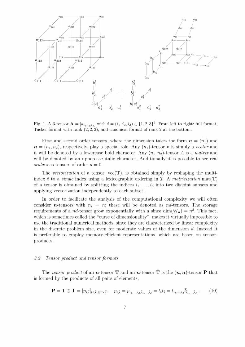
of order d and dimension n is an array consisting of real elements ti = ti1,...,id ∈ R withindices i = (i1, . . . , id) ∈ I, i.e., ik ∈ Ik, k = 1, . . . , d. For example, the elements of a(3, 3, 3)-tensor are visualized in Fig. 1. The number of elements

π(n) = n1 · · ·nd

is called the size of the tensor. The set of n-tensors forms the linear space Wn, equippedwith the Euclidean scalar product.

6

a111 a211 a311

a321

a331

a332

a333a233a133

a123 a223

a232a132a213a113 a313

a222 a322a122

a131a212

a121 a221

a312a231

a323

a112

g212g112

g111 g211

g122 g222

g221g212

a11 a21

b21

b22

b23b11

b12

b13

a12

a13

a22

a23

c23

c13

c22

c12c11

c21

b11a12 a13

b13c13

c12b12

a11c11 b21

a22 a23

b23c23

c22b22

a21c21

Fig. 1. A 3-tensor A = [ai1,i2,i3 ] with i = (i1, i2, i3) ∈ 1, 2, 33. From left to right: full format,Tucker format with rank (2, 2, 2), and canonical format of rank 2 at the bottom.

First and second order tensors, where the dimension takes the form n = (n1) andn = (n1, n2), respectively, play a special role. Any (n1)-tensor v is simply a vector andit will be denoted by a lowercase bold character. Any (n1, n2)-tensor A is a matrix andwill be denoted by an uppercase italic character. Additionally it is possible to see realscalars as tensors of order d = 0.

The vectorization of a tensor, vec(T), is obtained simply by reshaping the multi-index i to a single index using a lexicographic ordering in I. A matricization mat(T)of a tensor is obtained by splitting the indices i1, . . . , id into two disjoint subsets andapplying vectorization independently to each subset.

In order to facilitate the analysis of the computational complexity we will oftenconsider n-tensors with ni = n; these will be denoted as nd-tensors. The storagerequirements of a nd-tensor grow exponentially with d since dim(Wn) = nd. This fact,which is sometimes called the “curse of dimensionality”, makes it virtually impossible touse the traditional numerical methods, since they are characterized by linear complexityin the discrete problem size, even for moderate values of the dimension d. Instead itis preferable to employ memory-efficient representations, which are based on tensor-products.

3.2 Tensor product and tensor formats

The tensor product of an n-tensor T and an n-tensor T is the (n, n)-tensor P thatis formed by the products of all pairs of elements,

P = T⊗ T = [pi,i](i,i)∈I×I , pi,i = pi1,...,id ,i1,...,id = titi = ti1,...,id ti1,...,id . (10)

7

Moreover, the tensor product

Q =d⊗

k=1

v(k) with elements qi1,...,id =d∏

k=1

v(k)ik

(11)

of d vectors v(k) of dimensions nk, where k = 1, . . . , d, is an n = (n1, . . . , nd)-tensor, isreferred to as a rank-1 tensor. Note that the storage costs of this tensor scales linearlyin the order d.

Multiplication by scalars, which are seen as tensors of order 0, is a special case ofthe tensor product, where one usually omits the ⊗ sign. It satisfies the identity k∏

j=1

s(j)

k⊗j=1

T(j)

=k⊗j=1

(s(j)T(j)

). (12)

Using the tensor product leads to memory-efficient representations of tensors. In ourpaper we use the two main formats (or representations) which are common in theliterature:

• The R-term canonical representation of a tensor takes the form

T = [ti] =R∑r=1

d⊗k=1

v(k,r), i.e., ti = ti1,...,id =R∑r=1

d∏k=1

v(k,r)ik

, (13)

and is parameterized by Rd vectors v(k,r) ∈ Rnk . Clearly, any tensor admits a canonicalrepresentation for a sufficiently large value of R. The smallest integer R such that agiven tensor T admits such a representation is called its (canonical) rank R. If annd-tensor has rank R or lower, then its storage cost is bounded by Rnd.

An important special case is R = 1, where the representation takes the form (11).Tensors admitting a rank-1 representation are said to be separable.

In the case of matrices, the singular value decomposition (SVD) creates a canonicalrepresentation, where the rank R is equal to the number of non-zero singular valuesand the vectors v(k,r) are the left and right singular vectors scaled by the square rootsof the singular values.• A more general representation is the Tucker format

T = [ti] =ρ1∑r1=1

ρd∑rd=1

cr1,...,rd

d⊗k=1

v(k,rk), i.e., ti = ti1,...,id =ρ1∑r1=1

ρd∑rd=1

cr1,...,rd

d∏k=1

v(k,rk)ik

.

(14)which is defined by specifying the, so called, multi-rank ρ = (ρ1, . . . , ρd), the ρ1 +· · · + ρd vectors v(k,rk) ∈ Rnk and the core tensor C = [cr] of order d and dimensionρ. The storage cost is bounded by dρn + ρd with ρ = maxk ρk. This format becomesidentical to the canonical format when choosing ρk = R and considering a diagonalcore tensor C.

In the remainder of the paper we will focus mostly on the canonical representation.However, a representation in the Tucker format can be converted into a canonicalrepresentation, and vice versa. Notice that the maximal canonical rank of a tensor is

8

bounded by π(n)/maxnk, while the canonical rank of the Tucker tensor does notexceed π(ρ)/maxρk.

The rank-structured tensors with controllable complexity (i.e., the set of tensors incanonical or Tucker formats with bounded rank) form a manifold S ⊂Wn [26]. In orderto reduce the complexity of computations with tensors, we need to find approximaterepresentations of general tensors in this manifold, by performing a projection into S.This projection takes the form of the tensor truncation operator

TS : Wn → S : TSA = argminU∈S

‖A−U‖, (15)

which leads to a non-linear optimization problem, which is usually solved only approxi-mately.

A quasi-optimal rank-ρ approximation in the Tucker format is provided by the high-er-order SVD (HOSVD) algorithm [18]. The reduced HOSVD algorithm [40] efficientlyperforms tensor truncation to the canonical representation for moderate dimensions. Inthis situation one obtains a canonical representation of rank bounded by R = ρd−1 =O(| log ε|d−1 logd−1 n). A further reduction of the canonical rank can obtained by invokingthe alternating least-squares (ALS) method [41] for non-linear approximation.

3.3 Binary operations on tensors

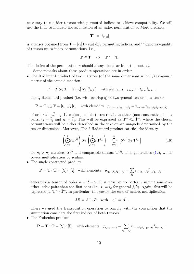
Besides the tensor product, numerous product operations for tensors are available.They can be defined by restricting the tensor product to elements with indices sat-isfying certain conditions, by (additionally) applying summation to certain subsets ofthe elements of the tensor product (10). We will use the operations which are listed inTable 1.

Table 1Selected binary operations for two tensors T ∈ Wn and T ∈ Wn with indices i and i,respectively.

Name symbol order of result obtained from the tensorproduct (10) by

compatibilityrequires

Hadamard q d + d− q restriction to indices withik = ik, k = 1, . . . , q

d, d ≥ q and nk = nkfor k = 1, . . . , q.

contracted · d + d− 2 summation over indiceswith i1 = i1

n1 = n1

Frobenius : d− d summation over indiceswith ik = ik, k = 1, . . . , d

d ≥ d and nk = nkfor k = 1, . . . , d.

Kronecker •× 2 matricization with respectto (i1, i1) and (i2, i2)

d = d = 2

Most of these operations are restricted to compatible pairs of tensors, and theKronecker product is even defined for pairs of matrices only. Sometimes it will be

9

necessary to consider tensors with permuted indices to achieve compatibility. We willuse the tilde to indicate the application of an index permutation σ. More precisely,

T∼ = [tσ(i)]

is a tensor obtained from T = [ti] by suitably permuting indices, and ∼= denotes equalityof tensors up to index permutations, i.e.,

T ∼= T ⇔ T∼ = T.

The choice of the permutation σ should always be clear from the context.

Some remarks about these product operations are in order:

• The Hadamard product of two matrices (of the same dimensions n1 × n2) is again amatrix of the same dimension,

P = T 2 T = [ti1,i2 ]2 [ti1,i2 ] with elements pi1,i2 = ti1,i2 ti1,i2 .

The q-Hadamard product (i.e. with overlap q) of two general tensors is a tensor

P = Tq T = [ti]q [ti] with elements pi1,...,id ,iq+1,...,id= ti1,...,id ti1,...,iq ,iq+1,...,id

of order d + d − q. It is also possible to restrict it to other (non-consecutive) indexpairs, ij = ij and ik = ik. This will be expressed as T∼ q T∼, where the chosenpermutations will be either described in the text or are uniquely determined by thetensor dimensions. Moreover, The 2-Hadamard product satisfies the identity k⊙

j=1

2 S(j)

2

k⊙j=1

2 T(j)

=k⊙j=1

2

[S(j) 2 T(j)

](16)

for n1 × n2 matrices S(j) and compatible tensors T(j). This generalizes (12), whichcovers multiplication by scalars.• The single contracted product

P = T · T = [ti] · [ti] with elements pi2,...,id ,i2,...,id =∑i1

ti1,i2,...,id ti1 ,i2,...,id .

generates a tensor of order d + d − 2. It is possible to perform summations overother index pairs than the first ones (i.e., ij = ik for general j, k). Again, this will beexpressed as T∼ · T∼. In particular, this covers the case of matrix multiplication,

AB = A∼ ·B with A∼ = A>,

where we used the transposition operation to comply with the convention that thesummation considers the first indices of both tensors.• The Frobenius product

P = T : T = [ti] : [ti] with elements pid+1,...,id=

∑i1,...,id

ti1,...,id,id+1,...,idti1,...,id .

10

performs summation with respect to as many index pairs as possible, where this isdetermined by the order of the second factor, which is assumed to be not exceed theorder of the first one. Again it is possible to consider other sequences of pairs of indices.

This product gives a scalar number if both factors have the same order and dimen-sion. It thus defines an inner product on Wn in this case.

The Frobenius product of separable tensors of the same dimensions satisfies theuseful identity (

d⊗i=1

v(i)

):

(d⊗i=1

v(i)

)=

d∏i=1

(v(i) · v(i)). (17)

• The Kronecker product

A •× A =

a11A · · · a1,n2A

.... . .

...

an1,1A · · · an1,n2A

, (18)

is only defined for pairs of matrices. It is a particular matricization of the tensorproduct of the two matrices A and A. The Kronecker product is a non-commutativeoperation.

4 Tensor functions

We proceed from tensors to functions with tensor-product structure. Tensor-productB-splines naturally fall into this category. Interestingly, there is a strong link betweenrank-1 tensors and multivariate functions which are products of univariate functions.

4.1 Tensor-product B-splines

We consider d possibly different univariate spline spaces Spkτkwith variables ξ(k),

k = 1, . . . , d. Each space is defined by a knot-vector τ k and a degree pk. The standardbasis of Spkτk

consists of the B-splines of degree pk, which are associated with the knotsτ k, see [50]. We collect the basis functions in the vector

β(k)(ξ(k)) =[β

(k)ik

(ξ(k))]

, ξ(k) ∈ [ak, bk] , k = 1 . . . d ,

which has the index set Ik possessing nk = #τ k − pk − 1 elements. More precisely, weobtain a vector (i.e., an element of Rnk) for any given value of the argument ξ(k). Forany such value, at most pk + 1 elements of the vector take non-zero values.

Given a coefficient vector c(k), a spline function fk ∈ Spkτkcan be represented using

the inner product,fk(ξ

(k)) = c(k) · β(k)(ξ(k)).

We will omit the argument ξ(k) if no confusion can arise.

11

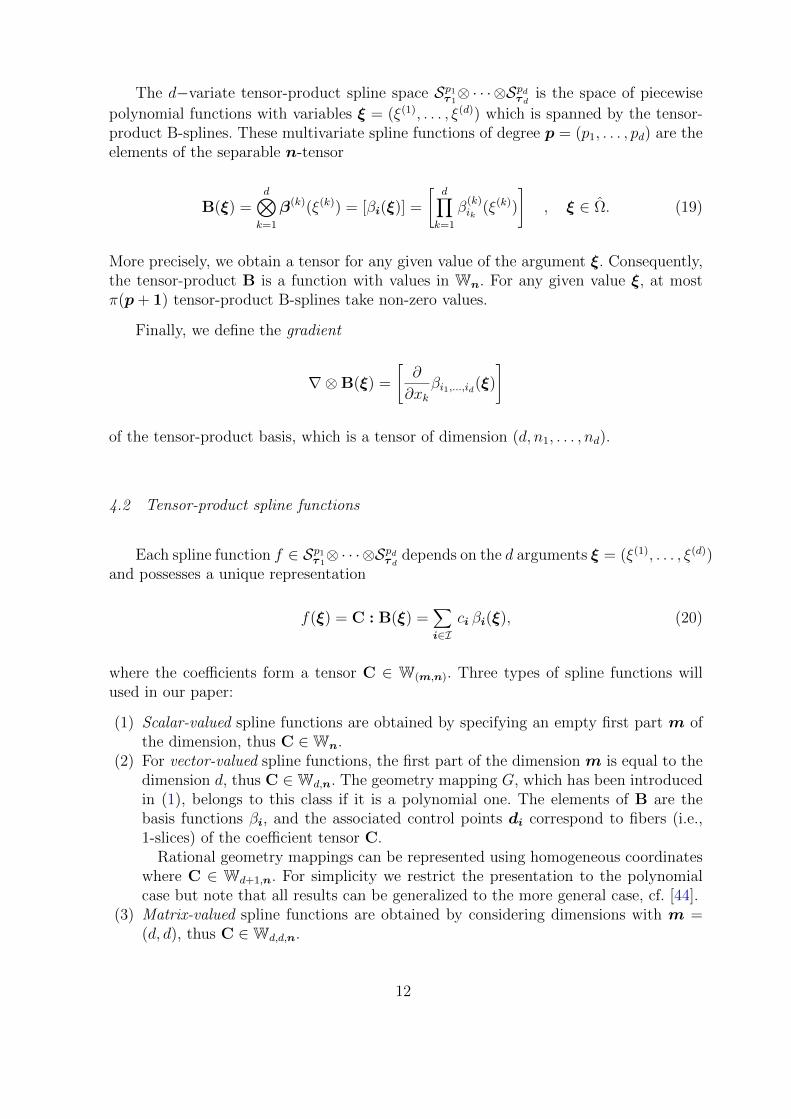
The d−variate tensor-product spline space Sp1τ1⊗ · · ·⊗Spdτd

is the space of piecewise

polynomial functions with variables ξ = (ξ(1), . . . , ξ(d)) which is spanned by the tensor-product B-splines. These multivariate spline functions of degree p = (p1, . . . , pd) are theelements of the separable n-tensor

B(ξ) =d⊗

k=1

β(k)(ξ(k)) = [βi(ξ)] =

[d∏

k=1

β(k)ik

(ξ(k))

], ξ ∈ Ω. (19)

More precisely, we obtain a tensor for any given value of the argument ξ. Consequently,the tensor-product B is a function with values in Wn. For any given value ξ, at mostπ(p+ 1) tensor-product B-splines take non-zero values.

Finally, we define the gradient

∇⊗B(ξ) =

[∂

∂xkβi1,...,id(ξ)

]

of the tensor-product basis, which is a tensor of dimension (d, n1, . . . , nd).

4.2 Tensor-product spline functions

Each spline function f ∈ Sp1τ1⊗ · · ·⊗Spdτd

depends on the d arguments ξ = (ξ(1), . . . , ξ(d))and possesses a unique representation

f(ξ) = C : B(ξ) =∑i∈I

ci βi(ξ), (20)

where the coefficients form a tensor C ∈ W(m,n). Three types of spline functions willused in our paper:

(1) Scalar-valued spline functions are obtained by specifying an empty first part m ofthe dimension, thus C ∈Wn.

(2) For vector-valued spline functions, the first part of the dimension m is equal to thedimension d, thus C ∈Wd,n. The geometry mapping G, which has been introducedin (1), belongs to this class if it is a polynomial one. The elements of B are thebasis functions βi, and the associated control points di correspond to fibers (i.e.,1-slices) of the coefficient tensor C.

Rational geometry mappings can be represented using homogeneous coordinateswhere C ∈ Wd+1,n. For simplicity we restrict the presentation to the polynomialcase but note that all results can be generalized to the more general case, cf. [44].

(3) Matrix-valued spline functions are obtained by considering dimensions with m =(d, d), thus C ∈Wd,d,n.

12

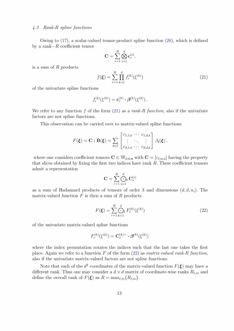
4.3 Rank-R spline functions

Owing to (17), a scalar-valued tensor-product spline function (20), which is definedby a rank−R coefficient tensor

C =R∑r=1

d⊗i=1

c(i)r ,

is a sum of R products

f(ξ) =R∑r=1

d∏k=1

f (k)r (ξ(k)) (21)

of the univariate spline functions

f (k)r (ξ(k)) = c(k)

r · β(k)(ξ(k)) .

We refer to any function f of the form (21) as a rank-R function, also if the univariatefactors are not spline functions.

This observation can be carried over to matrix-valued spline functions

F (ξ) = C : B(ξ) =∑i∈I

c1,1,i · · · c1,d,i...

. . ....

cd,1,i · · · cd,d,i

βi(ξ) ,

where one considers coefficient tensors C ∈Wd,d,n with C = [c`,m,i] having the propertythat slices obtained by fixing the first two indices have rank R. These coefficient tensorsadmit a representation

C =R∑r=1

d⊙i=1

2 C(i)r

as a sum of Hadamard products of tensors of order 3 and dimensions (d, d, ni). Thematrix-valued function F is then a sum of R products

F (ξ) =R∑r=1

d⊙k=1

2 F(k)r (ξ(k)) (22)

of the univariate matrix-valued spline functions

F (k)r (ξ(k)) = C(k)

r∼ · β(k)(ξ(k))

where the index permutation rotates the indices such that the last one takes the firstplace. Again we refer to a function F of the form (22) as matrix-valued rank-R function,also if the univariate matrix-valued factors are not spline functions.

Note that each of the d2 coordinates of the matrix-valued function F (ξ) may have adifferent rank. Thus one may consider a d× d matrix of coordinate-wise ranks R`,m anddefine the overall rank of F (ξ) as R = max`,mR`,m.

13

5 Tensor isogeometric analysis

We use tensor notation to express the entries of Galerkin matrices. Then we considerkernel functions of the rank-R and derive a compact Kronecker format for the mass andstiffness matrices.

5.1 Mass and stiffness tensors

The (element-wise) integral

P =∫

ΩT(ξ) dξ with elements pi =

∫Ωti(ξ) dξ (23)

of a tensor-valued function T = T(ξ) = [ti(ξ)] with the variable ξ ∈ Ω is obtained byapplying the integration to its entries. Integration commutes with multiplication in thefollowing sense: the integral of a tensor or Hadamard product of d tensors T(k)(ξ(k)),where the k-th one depends on ξ(k) only, inherits the product structure,

∫Ω

d⊙•×k=1

T(k)(ξ(k)) dξ =d⊙•×k=1

∫ bk

ak

T(k)(ξ(k)) dξ(k), •× = ⊗ or q . (24)

Clearly we need to assume compatible dimensions for the Hadamard product.

We define the mass tensor

M =∫

Ωω B︸︷︷︸

=[βi]

⊗ B︸︷︷︸=[βj ]

dξ ∈W(n,n), (25)

where the scalar ω = |det∇G| is determined by the geometry mapping. Note that theintegrand is a tensor, see (23). The associated mass matrix M = mat M ∈ Rπ(n)×π(n)

is obtained by performing matricization with respect to the indices i and j.

In addition we consider the stiffness tensor

S =∫

Ω[K · (∇⊗B)] · (∇⊗B) dξ ∈W(n,n), (26)

where the matrix K = [κ`,m] ∈ Rd×d is again determined by the geometry mapping,

K = ∇G−1∇G−T | det∇G|. (27)

Using the auxiliary d× d-matrix 1 = [1]`,m=1,...,d with all elements being equal to 1 andthe identity

[K · (v ⊗A′)] · (v′ ⊗A′) = K 2 [v ⊗ v′ ⊗A⊗A′] : 1,

we rewrite the stiffness tensor in the form

S = P : 1 . (28)

14

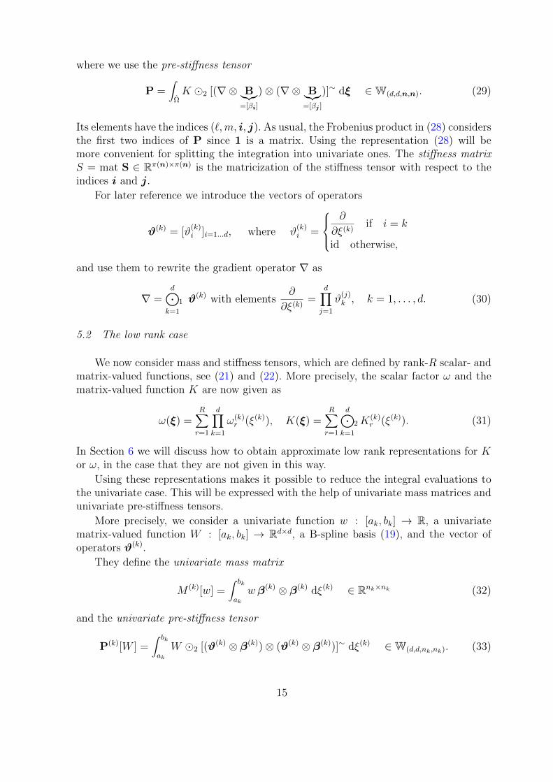
where we use the pre-stiffness tensor

P =∫

ΩK 2 [(∇⊗ B︸︷︷︸

=[βi]

)⊗ (∇⊗ B︸︷︷︸=[βj ]

)]∼ dξ ∈W(d,d,n,n). (29)

Its elements have the indices (`,m, i, j). As usual, the Frobenius product in (28) considersthe first two indices of P since 1 is a matrix. Using the representation (28) will bemore convenient for splitting the integration into univariate ones. The stiffness matrixS = mat S ∈ Rπ(n)×π(n) is the matricization of the stiffness tensor with respect to theindices i and j.

For later reference we introduce the vectors of operators

ϑ(k) = [ϑ(k)i ]i=1...d, where ϑ

(k)i =

∂

∂ξ(k)if i = k

id otherwise,

and use them to rewrite the gradient operator ∇ as

∇ =d⊙

k=1

1 ϑ(k) with elements

∂

∂ξ(k)=

d∏j=1

ϑ(j)k , k = 1, . . . , d. (30)

5.2 The low rank case

We now consider mass and stiffness tensors, which are defined by rank-R scalar- andmatrix-valued functions, see (21) and (22). More precisely, the scalar factor ω and thematrix-valued function K are now given as

ω(ξ) =R∑r=1

d∏k=1

ω(k)r (ξ(k)), K(ξ) =

R∑r=1

d⊙k=1

2K(k)r (ξ(k)). (31)

In Section 6 we will discuss how to obtain approximate low rank representations for Kor ω, in the case that they are not given in this way.

Using these representations makes it possible to reduce the integral evaluations tothe univariate case. This will be expressed with the help of univariate mass matrices andunivariate pre-stiffness tensors.

More precisely, we consider a univariate function w : [ak, bk] → R, a univariatematrix-valued function W : [ak, bk] → Rd×d, a B-spline basis (19), and the vector ofoperators ϑ(k).

They define the univariate mass matrix

M (k)[w] =∫ bk

ak

wβ(k) ⊗ β(k) dξ(k) ∈ Rnk×nk (32)

and the univariate pre-stiffness tensor

P(k)[W ] =∫ bk

ak

W 2 [(ϑ(k) ⊗ β(k))⊗ (ϑ(k) ⊗ β(k))]∼ dξ(k) ∈W(d,d,nk,nk). (33)

15

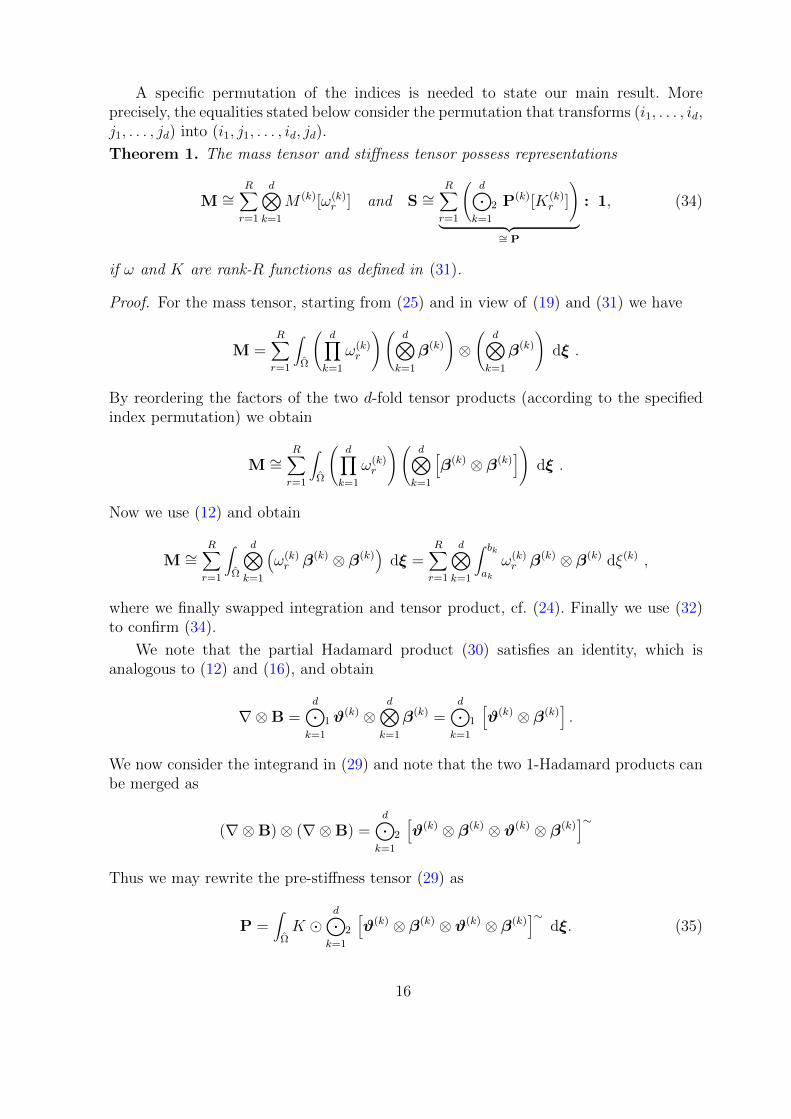
A specific permutation of the indices is needed to state our main result. Moreprecisely, the equalities stated below consider the permutation that transforms (i1, . . . , id,j1, . . . , jd) into (i1, j1, . . . , id, jd).

Theorem 1. The mass tensor and stiffness tensor possess representations

M ∼=R∑r=1

d⊗k=1

M (k)[ω(k)r ] and S ∼=

R∑r=1

(d⊙

k=1

2 P(k)[K(k)r ]

)︸ ︷︷ ︸

∼= P

: 1, (34)

if ω and K are rank-R functions as defined in (31).

Proof. For the mass tensor, starting from (25) and in view of (19) and (31) we have

M =R∑r=1

∫Ω

(d∏

k=1

ω(k)r

)(d⊗

k=1

β(k)

)⊗(

d⊗k=1

β(k)

)dξ .

By reordering the factors of the two d-fold tensor products (according to the specifiedindex permutation) we obtain

M ∼=R∑r=1

∫Ω

(d∏

k=1

ω(k)r

)(d⊗

k=1

[β(k) ⊗ β(k)

])dξ .

Now we use (12) and obtain

M ∼=R∑r=1

∫Ω

d⊗k=1

(ω(k)r β(k) ⊗ β(k)

)dξ =

R∑r=1

d⊗k=1

∫ bk

ak

ω(k)r β(k) ⊗ β(k) dξ(k) ,

where we finally swapped integration and tensor product, cf. (24). Finally we use (32)to confirm (34).

We note that the partial Hadamard product (30) satisfies an identity, which isanalogous to (12) and (16), and obtain

∇⊗B =d⊙

k=1

1 ϑ(k) ⊗

d⊗k=1

β(k) =d⊙

k=1

1

[ϑ(k) ⊗ β(k)

].

We now consider the integrand in (29) and note that the two 1-Hadamard products canbe merged as

(∇⊗B)⊗ (∇⊗B) =d⊙

k=1

2

[ϑ(k) ⊗ β(k) ⊗ ϑ(k) ⊗ β(k)

]∼Thus we may rewrite the pre-stiffness tensor (29) as

P =∫

ΩK

d⊙k=1

2

[ϑ(k) ⊗ β(k) ⊗ ϑ(k) ⊗ β(k)

]∼dξ. (35)

16

We now employ (31) and again (16) to obtain

P ∼=∫

Ω

R∑r=1

d⊙k=1

2

(K(k)r 2

[ϑ(k) ⊗ β(k) ⊗ ϑ(k) ⊗ β(k)

]∼)dξ. (36)

Finally we note that the products commute with integration (24) and use (28) and (33)to complete the proof.

A completely similar formulation can be derived for the advection matrix (8), or forother kinds of matrices appearing in a Galerkin discretization.

Recall that the mass and the stiffness matrices are specific matricizations of thecorresponding tensors, where one considers a lexicographic ordering of the indices. It isconvenient to express these matrices as a sum of Kronecker products. We do so in thefollowing

Corollary 2 (Kronecker format). We denote by P(k)`,m[K(k)

r ] ∈ Rnk×nk the matrix slices

of the univariate pre-stiffness tensors P(k)[K(k)r ]. The mass and stiffness matrices are

M =R∑r=1

d⊙•×k=1

M (k)[ω(k)r ] and S =

R∑r=1

d∑`,m=1

d⊙•×k=1

P(k)`,m[K(k)

r ] , (37)

provided that the identities (31) are satisfied.

Proof. The mass and stiffness matrices can be rewritten as

M =∫

Ωω vec B⊗ vec B dξ and S =

∫Ω

[K · (∇⊗ vec B)] · (∇⊗ vec B) dξ .

One may use the identity

vec

(d⊗i=1

v(i)

)⊗ vec

(d⊗i=1

v(i)

)=

d⊙•×i=1

(v(i) ⊗ v(i)

),

which allows to represent the tensor product of vectorized rank-1 tensors as the Kro-necker product of the vector factors, to derive (37).

We will refer to the representation (37), which expresses the mass and stiffnessmatrices as a sum of Kronecker products of smaller matrices, which are obtained byunivariate integrations, as the Kronecker format of the matrices. Moreover, the numberof summands will be referred to as the Kronecker rank of the matrix, see also [28]. Notethat this notion of rank is different from the usual matrix rank.

Example 3. Consider a volumetric domain Ω, given as the image of the parametricmap

G : [0, 1]3 → R3 with (x, y, z) 7→ G(ξ) =((x2 − 1)(y + 1), (x+ 1)(y + 1), z

).

where we use the abbreviations ξ(1) = x, ξ(2) = y, ξ(3) = z. For the sake of simplicity wework with the monomial basis, instead of using B-splines. We consider a single element

17

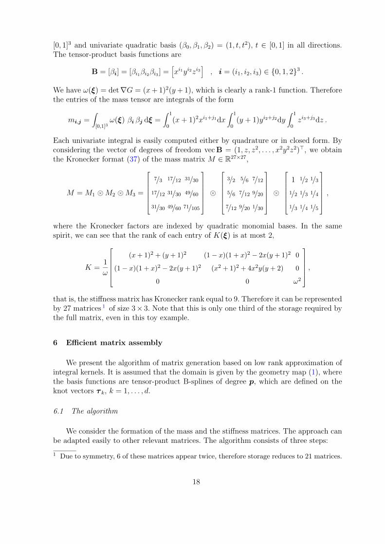
[0, 1]3 and univariate quadratic basis (β0, β1, β2) = (1, t, t2), t ∈ [0, 1] in all directions.The tensor-product basis functions are

B = [βi] = [βi1βi2βi3 ] =[xi1yi2zi3

], i = (i1, i2, i3) ∈ 0, 1, 23 .

We have ω(ξ) = det∇G = (x+ 1)2(y+ 1), which is clearly a rank-1 function. Thereforethe entries of the mass tensor are integrals of the form

mi,j =∫

[0,1]3ω(ξ) βi βj dξ =

∫ 1

0(x+ 1)2xi1+j1dx

∫ 1

0(y + 1)yi2+j2dy

∫ 1

0zi3+j3dz .

Each univariate integral is easily computed either by quadrature or in closed form. Byconsidering the vector of degrees of freedom vec B = (1, z, z2, . . . , x2y2z2)>, we obtainthe Kronecker format (37) of the mass matrix M ∈ R27×27,

M = M1 •× M2 •× M3 =

7/3 17/12 31/30

17/12 31/30 49/60

31/30 49/60 71/105

•×

3/2 5/6 7/12

5/6 7/12 9/20

7/12 9/20 1/30

•×

1 1/2 1/3

1/2 1/3 1/4

1/3 1/4 1/5

,

where the Kronecker factors are indexed by quadratic monomial bases. In the samespirit, we can see that the rank of each entry of K(ξ) is at most 2,

K =1

ω

(x + 1)2 + (y + 1)2 (1− x)(1 + x)2 − 2x(y + 1)2 0

(1− x)(1 + x)2 − 2x(y + 1)2 (x2 + 1)2 + 4x2y(y + 2) 0

0 0 ω2

,

that is, the stiffness matrix has Kronecker rank equal to 9. Therefore it can be representedby 27 matrices 1 of size 3× 3. Note that this is only one third of the storage required bythe full matrix, even in this toy example.

6 Efficient matrix assembly

We present the algorithm of matrix generation based on low rank approximation ofintegral kernels. It is assumed that the domain is given by the geometry map (1), wherethe basis functions are tensor-product B-splines of degree p, which are defined on theknot vectors τ k, k = 1, . . . , d.

6.1 The algorithm

We consider the formation of the mass and the stiffness matrices. The approach canbe adapted easily to other relevant matrices. The algorithm consists of three steps:

1 Due to symmetry, 6 of these matrices appear twice, therefore storage reduces to 21 matrices.

18

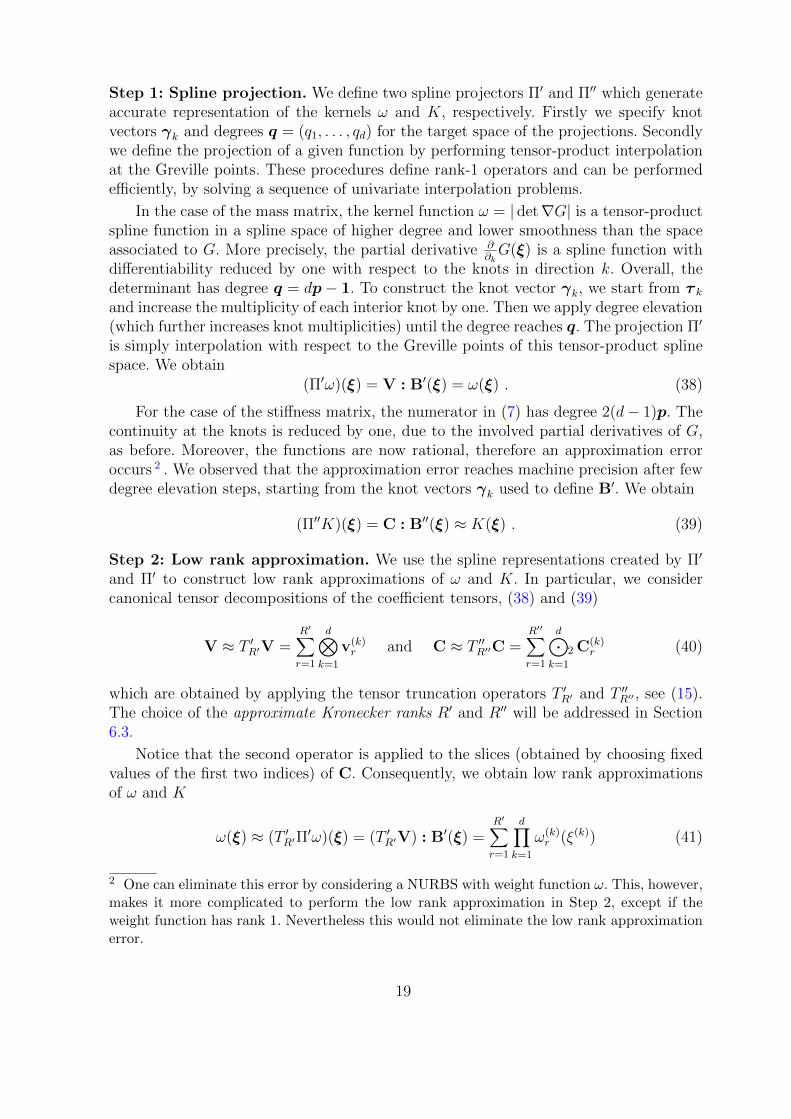
Step 1: Spline projection. We define two spline projectors Π′ and Π′′ which generateaccurate representation of the kernels ω and K, respectively. Firstly we specify knotvectors γk and degrees q = (q1, . . . , qd) for the target space of the projections. Secondlywe define the projection of a given function by performing tensor-product interpolationat the Greville points. These procedures define rank-1 operators and can be performedefficiently, by solving a sequence of univariate interpolation problems.

In the case of the mass matrix, the kernel function ω = | det∇G| is a tensor-productspline function in a spline space of higher degree and lower smoothness than the spaceassociated to G. More precisely, the partial derivative ∂

∂kG(ξ) is a spline function with

differentiability reduced by one with respect to the knots in direction k. Overall, thedeterminant has degree q = dp− 1. To construct the knot vector γk, we start from τ kand increase the multiplicity of each interior knot by one. Then we apply degree elevation(which further increases knot multiplicities) until the degree reaches q. The projection Π′

is simply interpolation with respect to the Greville points of this tensor-product splinespace. We obtain

(Π′ω)(ξ) = V : B′(ξ) = ω(ξ) . (38)

For the case of the stiffness matrix, the numerator in (7) has degree 2(d− 1)p. Thecontinuity at the knots is reduced by one, due to the involved partial derivatives of G,as before. Moreover, the functions are now rational, therefore an approximation erroroccurs 2 . We observed that the approximation error reaches machine precision after fewdegree elevation steps, starting from the knot vectors γk used to define B′. We obtain

(Π′′K)(ξ) = C : B′′(ξ) ≈ K(ξ) . (39)

Step 2: Low rank approximation. We use the spline representations created by Π′

and Π′ to construct low rank approximations of ω and K. In particular, we considercanonical tensor decompositions of the coefficient tensors, (38) and (39)

V ≈ T ′R′V =R′∑r=1

d⊗k=1

v(k)r and C ≈ T ′′R′′C =

R′′∑r=1

d⊙k=1

2 C(k)r (40)

which are obtained by applying the tensor truncation operators T ′R′ and T ′′R′′ , see (15).The choice of the approximate Kronecker ranks R′ and R′′ will be addressed in Section6.3.

Notice that the second operator is applied to the slices (obtained by choosing fixedvalues of the first two indices) of C. Consequently, we obtain low rank approximationsof ω and K

ω(ξ) ≈ (T ′R′Π′ω)(ξ) = (T ′R′V) : B′(ξ) =

R′∑r=1

d∏k=1

ω(k)r (ξ(k)) (41)

2 One can eliminate this error by considering a NURBS with weight function ω. This, however,makes it more complicated to perform the low rank approximation in Step 2, except if theweight function has rank 1. Nevertheless this would not eliminate the low rank approximationerror.

19

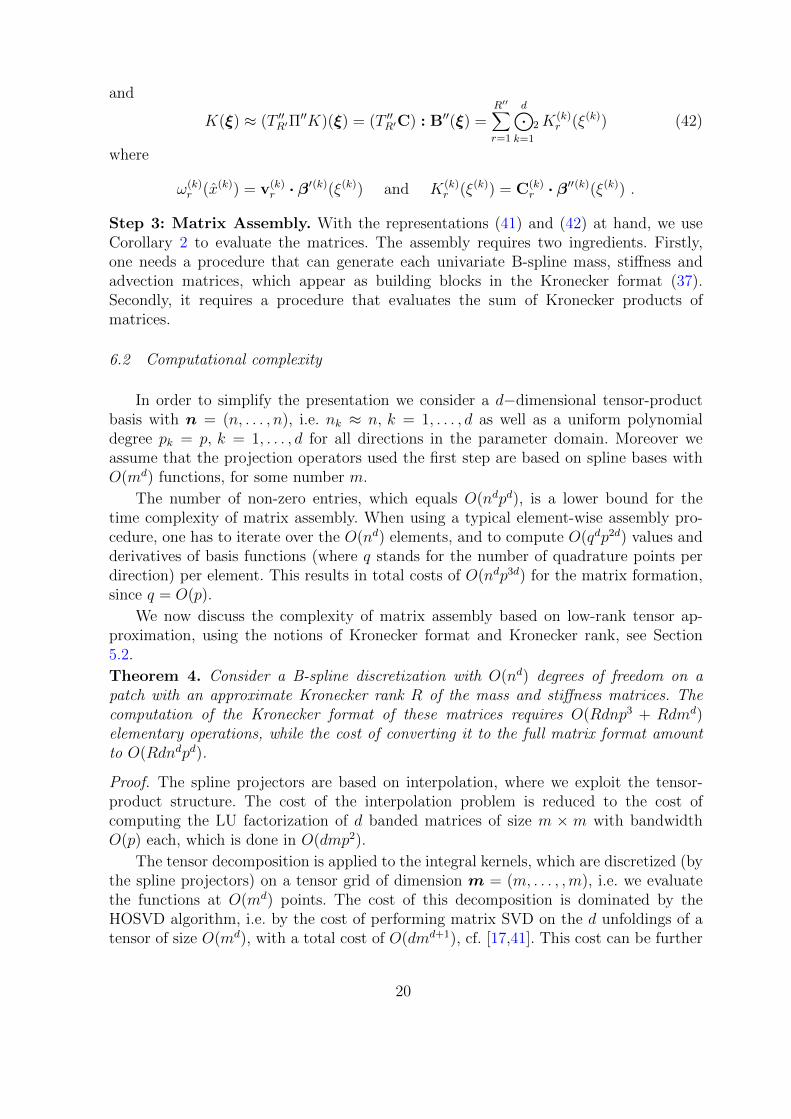
and

K(ξ) ≈ (T ′′R′Π′′K)(ξ) = (T ′′R′C) : B′′(ξ) =

R′′∑r=1

d⊙k=1

2K(k)r (ξ(k)) (42)

where

ω(k)r (x(k)) = v(k)

r · β′(k)(ξ(k)) and K(k)r (ξ(k)) = C(k)

r · β′′(k)(ξ(k)) .

Step 3: Matrix Assembly. With the representations (41) and (42) at hand, we useCorollary 2 to evaluate the matrices. The assembly requires two ingredients. Firstly,one needs a procedure that can generate each univariate B-spline mass, stiffness andadvection matrices, which appear as building blocks in the Kronecker format (37).Secondly, it requires a procedure that evaluates the sum of Kronecker products ofmatrices.

6.2 Computational complexity

In order to simplify the presentation we consider a d−dimensional tensor-productbasis with n = (n, . . . , n), i.e. nk ≈ n, k = 1, . . . , d as well as a uniform polynomialdegree pk = p, k = 1, . . . , d for all directions in the parameter domain. Moreover weassume that the projection operators used the first step are based on spline bases withO(md) functions, for some number m.

The number of non-zero entries, which equals O(ndpd), is a lower bound for thetime complexity of matrix assembly. When using a typical element-wise assembly pro-cedure, one has to iterate over the O(nd) elements, and to compute O(qdp2d) values andderivatives of basis functions (where q stands for the number of quadrature points perdirection) per element. This results in total costs of O(ndp3d) for the matrix formation,since q = O(p).

We now discuss the complexity of matrix assembly based on low-rank tensor ap-proximation, using the notions of Kronecker format and Kronecker rank, see Section5.2.

Theorem 4. Consider a B-spline discretization with O(nd) degrees of freedom on apatch with an approximate Kronecker rank R of the mass and stiffness matrices. Thecomputation of the Kronecker format of these matrices requires O(Rdnp3 + Rdmd)elementary operations, while the cost of converting it to the full matrix format amountto O(Rdndpd).

Proof. The spline projectors are based on interpolation, where we exploit the tensor-product structure. The cost of the interpolation problem is reduced to the cost ofcomputing the LU factorization of d banded matrices of size m × m with bandwidthO(p) each, which is done in O(dmp2).

The tensor decomposition is applied to the integral kernels, which are discretized (bythe spline projectors) on a tensor grid of dimension m = (m, . . . , ,m), i.e. we evaluatethe functions at O(md) points. The cost of this decomposition is dominated by theHOSVD algorithm, i.e. by the cost of performing matrix SVD on the d unfoldings of atensor of size O(md), with a total cost of O(dmd+1), cf. [17,41]. This cost can be further

20

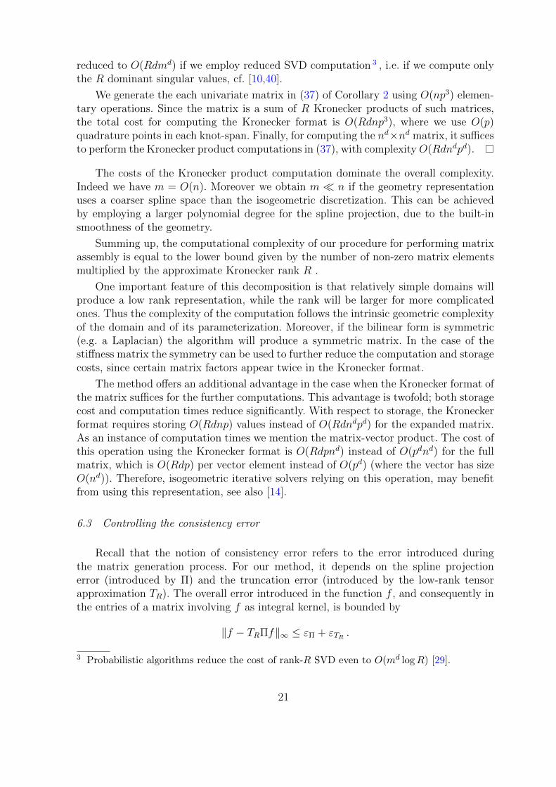
reduced to O(Rdmd) if we employ reduced SVD computation 3 , i.e. if we compute onlythe R dominant singular values, cf. [10,40].

We generate the each univariate matrix in (37) of Corollary 2 using O(np3) elemen-tary operations. Since the matrix is a sum of R Kronecker products of such matrices,the total cost for computing the Kronecker format is O(Rdnp3), where we use O(p)quadrature points in each knot-span. Finally, for computing the nd×nd matrix, it sufficesto perform the Kronecker product computations in (37), with complexityO(Rdndpd).

The costs of the Kronecker product computation dominate the overall complexity.Indeed we have m = O(n). Moreover we obtain m n if the geometry representationuses a coarser spline space than the isogeometric discretization. This can be achievedby employing a larger polynomial degree for the spline projection, due to the built-insmoothness of the geometry.

Summing up, the computational complexity of our procedure for performing matrixassembly is equal to the lower bound given by the number of non-zero matrix elementsmultiplied by the approximate Kronecker rank R .

One important feature of this decomposition is that relatively simple domains willproduce a low rank representation, while the rank will be larger for more complicatedones. Thus the complexity of the computation follows the intrinsic geometric complexityof the domain and of its parameterization. Moreover, if the bilinear form is symmetric(e.g. a Laplacian) the algorithm will produce a symmetric matrix. In the case of thestiffness matrix the symmetry can be used to further reduce the computation and storagecosts, since certain matrix factors appear twice in the Kronecker format.

The method offers an additional advantage in the case when the Kronecker format ofthe matrix suffices for the further computations. This advantage is twofold; both storagecost and computation times reduce significantly. With respect to storage, the Kroneckerformat requires storing O(Rdnp) values instead of O(Rdndpd) for the expanded matrix.As an instance of computation times we mention the matrix-vector product. The cost ofthis operation using the Kronecker format is O(Rdpnd) instead of O(pdnd) for the fullmatrix, which is O(Rdp) per vector element instead of O(pd) (where the vector has sizeO(nd)). Therefore, isogeometric iterative solvers relying on this operation, may benefitfrom using this representation, see also [14].

6.3 Controlling the consistency error

Recall that the notion of consistency error refers to the error introduced duringthe matrix generation process. For our method, it depends on the spline projectionerror (introduced by Π) and the truncation error (introduced by the low-rank tensorapproximation TR). The overall error introduced in the function f , and consequently inthe entries of a matrix involving f as integral kernel, is bounded by

‖f − TRΠf‖∞ ≤ εΠ + εTR .

3 Probabilistic algorithms reduce the cost of rank-R SVD even to O(md logR) [29].

21

With this error bound at hand, the same approach as in [44, Th. 13] can be employedto derive consistency error bounds for Galerkin discretization of the particular bilinearforms. We shall verify experimentally in Section 7 that optimal convergence rates areobtained.

The usual scenario for controlling the error is to set an a priori error tolerance and toensure that both contributions to the total error respect it. As already mentioned, in thegeneral case the rank is related to the desired accuracy by R = O(| log εTR |d−1 logd−1m),where m is the same as in Theorem 4. In particular in 2D, using R-truncated SVDimplies an error bounded by

εTR ≤ 2√∑r>R

σ2r ,

where σr are the singular values ordered by decreasing magnitude.

Regarding the projection error, in general it should be chosen such that the overallaccuracy is maintained. For instance if Π uses uniform splines of degree q with m knotspans per direction, we have εΠ = O(m−q−1). To match, e.g., the L2 discretizationerror, which is for elliptic problems O(n−p−1) (for uniform grids), it suffices to choosem = n(p+1)/(q+1). Consequently for q ≈ dp we obtain m ≈ n1/d as the degree p increases.

Finally, small (negligible) integration error are introduced by the quadrature of the1D (mass or stiffness) integrals. The degree of these integrals is larger than 2p−1, whichis the exactness of the Gauss rule with p+1 nodes. Nevertheless, p+1 nodes per directionsuffice to reduce the error down to the order of the approximation error.

7 Experiments and numerical results

In this section we apply our method to a set of model shapes. We have developed aC++ implementation of the method in the G+Smo library 4 [35].

In what follows we examine the performance of tensor decomposition on the modelpatches, then we test the convergence rates obtained by our algorithm for problemsinvolving the mass and the stiffness matrices, as well as the effect of rank trunctation.

Moreover we compare computation times for matrix generation and for a simpleconjugate gradient solver when using the full matrix format and when using the (lowrank) Kronecker matrix format.

7.1 Tensor decomposition

In this section we examine the Kronecker-rank profile of some model geometries.The approximated quantities are the kernels appearing in the mass (6) and stiffness (7)integrals. The patches tested are shown in Table 2. For each shape, the degree p of theparameterization and the size of the control grid is indicated. Moreover, the Kroneckerrank of the integral kerners are shown, as well as the size of the tensor grid used forinterpolating the kernels.

4 Geometry plus simulation modules, http://gs.jku.at/gismo, 2016.

22

We use HOSVD to obtain a Tucker representation of the tensors and we convert itto a canonical representation. For obtaining an even lower canonical rank, we use ALSiteration in the process. We use successive rank-1 approximations of the residue as initialvalues for each step of the ALS iteration. In all computations, we set the accuracy toε = 10−8, and we stop the iteration as soon as the Frobenious norm of the residue isbelow ε.

Table 2 shows that the rank profile is related to the geometric complexity of thedomain. We know that in 2D the rank (computed by SVD) is limited by the minimumnumber of basis functions in the coordinate bases of the projection basis used in Π. In3D, the rank is bounded by the product of the two short dimensions in the core tensorof the HOSVD. Below the shape we note the (tensor) dimensions of the B-spline basisused for the geometry parameterization, as well as for projecting Ω and K, respectively.

The results reveal that the overall rank profile is correlated with the geometriccomplexity of the model, rather than the polynomial degree. In particular, patches whichare more symmetric have lower rank numbers, while irregular shapes (such as case (e))have more elevated rank numbers, even though the degree of the parameterization issmall.

We can observe that symmetric shapes or shapes with a polar parameterizationhave smaller rank values than shapes with arbitrary form. The correlation to the degreeof the parameterization is weaker. Indeed, the trilinear shape in (2e) has higher rankvalues than (2b), which is quadratic in all parametric directions. Note however thatthe bottom and top faces of (2e) are arranged in an arbitrary fashion, contrarily to themirror symmetry which is present in (2b).

We also tested the behaviour of the rank values when applying h−refinement to theprojection space. In all cases it is verified that the computed rank value is invariantunder h−refinement. This is an indication that these values are intrinsic propertiesof the underlying continuous functions ω or K, which in turn depend on the givenparameterization.

7.2 Order of convergence

In this section we use the models (2c) and (2f) and we consider the problem ofapproximating the function

f(x, y, z) = sin(πx) sin(πy) sin(πz) , (43)

in two scenarios. In the first one, we use the mass matrix for computing the L2 projectionof f(x, y, z) to the (k−refined) B-spline space obtained from the geometry representation.In the second scenario we consider the PDE −∆f = g, f = f0 on ∂Ω, where f0 and gare defined so that the exact solution is (43). This PDE is solved for the control pointsof the approximate solution using the computed stiffness matrix. A view of the functionon the two test domains is depicted in Figure 2.

As outlined in Section 6.3, the overall error is the sum of the discretization plusthe consistency (integration) error. We verify that the overall error is of the order

23

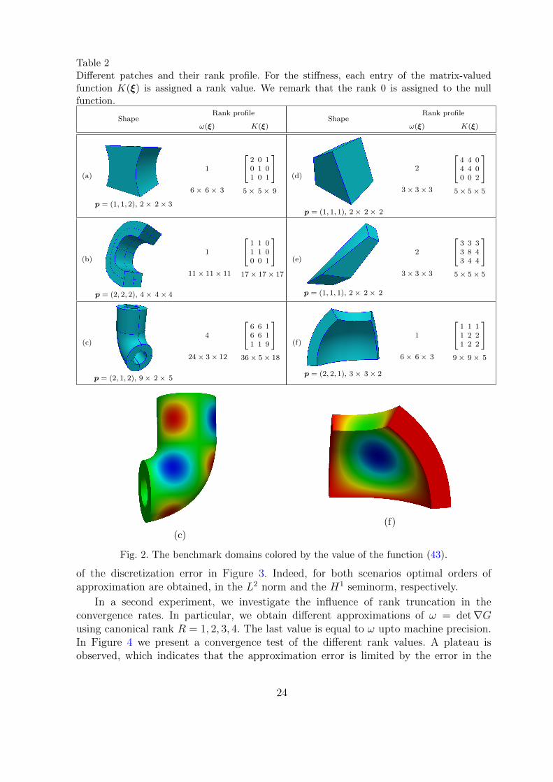
Table 2Different patches and their rank profile. For the stiffness, each entry of the matrix-valuedfunction K(ξ) is assigned a rank value. We remark that the rank 0 is assigned to the nullfunction.

ShapeRank profile

ω(ξ) K(ξ)

(a)

p = (1, 1, 2), 2× 2× 3

1

6× 6× 3

[2 0 10 1 01 0 1

]5× 5× 9

(b)

p = (2, 2, 2), 4× 4× 4

1

11× 11× 11

[1 1 01 1 00 0 1

]17× 17× 17

(c)

p = (2, 1, 2), 9× 2× 5

4

24× 3× 12

[6 6 16 6 11 1 9

]36× 5× 18

ShapeRank profile

ω(ξ) K(ξ)

(d)

p = (1, 1, 1), 2× 2× 2

2

3× 3× 3

[4 4 04 4 00 0 2

]5× 5× 5

(e)

p = (1, 1, 1), 2× 2× 2

2

3× 3× 3

[3 3 33 8 43 4 4

]5× 5× 5

(f)

p = (2, 2, 1), 3× 3× 2

1

6× 6× 3

[1 1 11 2 21 2 2

]9× 9× 5

(c)

(f)

Fig. 2. The benchmark domains colored by the value of the function (43).

of the discretization error in Figure 3. Indeed, for both scenarios optimal orders ofapproximation are obtained, in the L2 norm and the H1 seminorm, respectively.

In a second experiment, we investigate the influence of rank truncation in theconvergence rates. In particular, we obtain different approximations of ω = det∇Gusing canonical rank R = 1, 2, 3, 4. The last value is equal to ω upto machine precision.In Figure 4 we present a convergence test of the different rank values. A plateau isobserved, which indicates that the approximation error is limited by the error in the

24

1 1.5 22

4

6

8

345

− log(h)

−lo

g(‖f h−f‖ 2,Ω

)

L2 projection (R=1)

p = 2

p = 3

p = 4

0.5 1 1.50

2

4

6

234

− log(h)

−lo

g(|f

h−f| 1,

Ω)

Convergence in H1 seminorm (R=13)

p = 2

p = 3

p = 4

Fig. 3. Experimental orders of convergence for the L2 projection and Laplacian problems usinglow rank mass and stiffness approximation, for degrees p = 2, 3, 4. The domain Ω is the volumedepicted in Table 2f, and fh stands for the computed approximation of (43).

rank approximation. A higher rank value sets this limit to higher accuracy. For thevalue R = 4, the full convergence rate is obtained. This shows that the rank truncationerror is carried over to the final solution, therefore it has to be controlled with care toobtain high accuracy.

0.5 1 1.5−1

0

1

2

3

− log(h)

−lo

g(‖f h−f‖ 2,Ω

)

L2 projection (p=2)

R = 1

R = 2

R = 3

R = 4

0.5 1 1.5−1

0

1

2

3

4

− log(h)

−lo

g(‖f h−f‖ 2,Ω

)

L2 projection (p=3)

R = 1

R = 2

R = 3

R = 4

Fig. 4. Rank truncation effect: We apply L2 projection with approximate mass matrix usingdifferent ranks, for degrees p = 2 and p = 3. The domain used is the one shown in Table 2c.

7.3 Computation and storage costs for matrix assembly

In this section we examine the computation and storage costs of the two differentrepresentations. First, we look at the Kronecker matrix format (KF) and secondly weuse our algorithm to compute the (usual) standard format (SF) of the matrix, by takingKronecker products (KP).

25

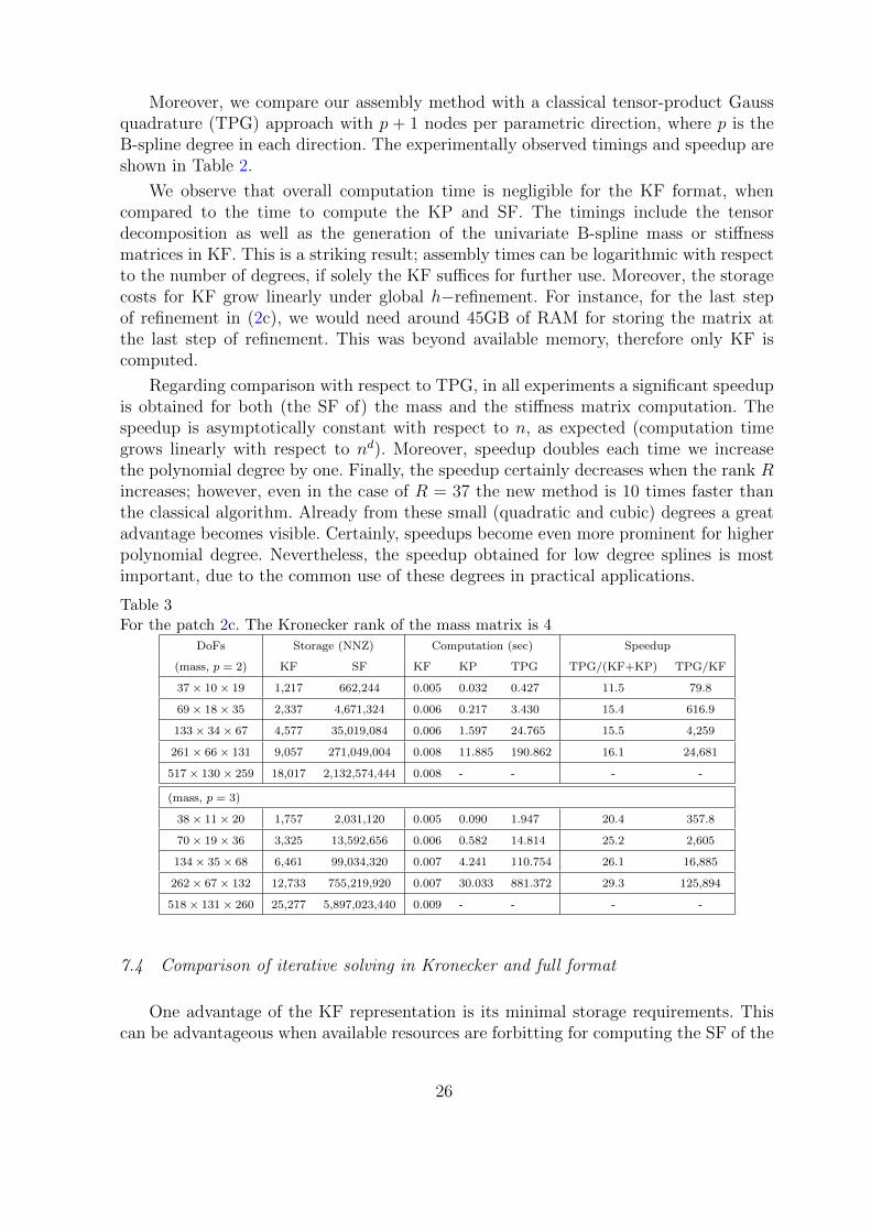
Moreover, we compare our assembly method with a classical tensor-product Gaussquadrature (TPG) approach with p + 1 nodes per parametric direction, where p is theB-spline degree in each direction. The experimentally observed timings and speedup areshown in Table 2.

We observe that overall computation time is negligible for the KF format, whencompared to the time to compute the KP and SF. The timings include the tensordecomposition as well as the generation of the univariate B-spline mass or stiffnessmatrices in KF. This is a striking result; assembly times can be logarithmic with respectto the number of degrees, if solely the KF suffices for further use. Moreover, the storagecosts for KF grow linearly under global h−refinement. For instance, for the last stepof refinement in (2c), we would need around 45GB of RAM for storing the matrix atthe last step of refinement. This was beyond available memory, therefore only KF iscomputed.

Regarding comparison with respect to TPG, in all experiments a significant speedupis obtained for both (the SF of) the mass and the stiffness matrix computation. Thespeedup is asymptotically constant with respect to n, as expected (computation timegrows linearly with respect to nd). Moreover, speedup doubles each time we increasethe polynomial degree by one. Finally, the speedup certainly decreases when the rank Rincreases; however, even in the case of R = 37 the new method is 10 times faster thanthe classical algorithm. Already from these small (quadratic and cubic) degrees a greatadvantage becomes visible. Certainly, speedups become even more prominent for higherpolynomial degree. Nevertheless, the speedup obtained for low degree splines is mostimportant, due to the common use of these degrees in practical applications.

Table 3For the patch 2c. The Kronecker rank of the mass matrix is 4

DoFs Storage (NNZ) Computation (sec) Speedup

(mass, p = 2) KF SF KF KP TPG TPG/(KF+KP) TPG/KF

37× 10× 19 1,217 662,244 0.005 0.032 0.427 11.5 79.8

69× 18× 35 2,337 4,671,324 0.006 0.217 3.430 15.4 616.9

133× 34× 67 4,577 35,019,084 0.006 1.597 24.765 15.5 4,259

261× 66× 131 9,057 271,049,004 0.008 11.885 190.862 16.1 24,681

517× 130× 259 18,017 2,132,574,444 0.008 - - - -

(mass, p = 3)

38× 11× 20 1,757 2,031,120 0.005 0.090 1.947 20.4 357.8

70× 19× 36 3,325 13,592,656 0.006 0.582 14.814 25.2 2,605

134× 35× 68 6,461 99,034,320 0.007 4.241 110.754 26.1 16,885

262× 67× 132 12,733 755,219,920 0.007 30.033 881.372 29.3 125,894

518× 131× 260 25,277 5,897,023,440 0.009 - - - -

7.4 Comparison of iterative solving in Kronecker and full format

One advantage of the KF representation is its minimal storage requirements. Thiscan be advantageous when available resources are forbitting for computing the SF of the

26

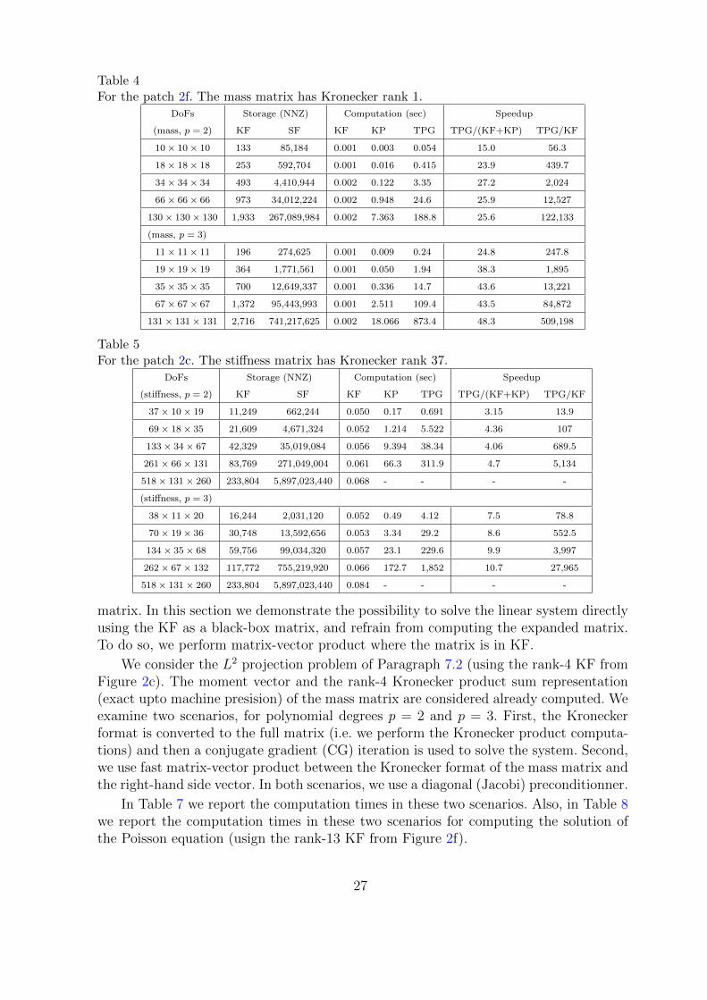
Table 4For the patch 2f. The mass matrix has Kronecker rank 1.

DoFs Storage (NNZ) Computation (sec) Speedup

(mass, p = 2) KF SF KF KP TPG TPG/(KF+KP) TPG/KF

10× 10× 10 133 85,184 0.001 0.003 0.054 15.0 56.3

18× 18× 18 253 592,704 0.001 0.016 0.415 23.9 439.7

34× 34× 34 493 4,410,944 0.002 0.122 3.35 27.2 2,024

66× 66× 66 973 34,012,224 0.002 0.948 24.6 25.9 12,527

130× 130× 130 1,933 267,089,984 0.002 7.363 188.8 25.6 122,133

(mass, p = 3)

11× 11× 11 196 274,625 0.001 0.009 0.24 24.8 247.8

19× 19× 19 364 1,771,561 0.001 0.050 1.94 38.3 1,895

35× 35× 35 700 12,649,337 0.001 0.336 14.7 43.6 13,221

67× 67× 67 1,372 95,443,993 0.001 2.511 109.4 43.5 84,872

131× 131× 131 2,716 741,217,625 0.002 18.066 873.4 48.3 509,198

Table 5For the patch 2c. The stiffness matrix has Kronecker rank 37.

DoFs Storage (NNZ) Computation (sec) Speedup

(stiffness, p = 2) KF SF KF KP TPG TPG/(KF+KP) TPG/KF

37× 10× 19 11,249 662,244 0.050 0.17 0.691 3.15 13.9

69× 18× 35 21,609 4,671,324 0.052 1.214 5.522 4.36 107

133× 34× 67 42,329 35,019,084 0.056 9.394 38.34 4.06 689.5

261× 66× 131 83,769 271,049,004 0.061 66.3 311.9 4.7 5,134

518× 131× 260 233,804 5,897,023,440 0.068 - - - -

(stiffness, p = 3)

38× 11× 20 16,244 2,031,120 0.052 0.49 4.12 7.5 78.8

70× 19× 36 30,748 13,592,656 0.053 3.34 29.2 8.6 552.5

134× 35× 68 59,756 99,034,320 0.057 23.1 229.6 9.9 3,997

262× 67× 132 117,772 755,219,920 0.066 172.7 1,852 10.7 27,965

518× 131× 260 233,804 5,897,023,440 0.084 - - - -

matrix. In this section we demonstrate the possibility to solve the linear system directlyusing the KF as a black-box matrix, and refrain from computing the expanded matrix.To do so, we perform matrix-vector product where the matrix is in KF.

We consider the L2 projection problem of Paragraph 7.2 (using the rank-4 KF fromFigure 2c). The moment vector and the rank-4 Kronecker product sum representation(exact upto machine presision) of the mass matrix are considered already computed. Weexamine two scenarios, for polynomial degrees p = 2 and p = 3. First, the Kroneckerformat is converted to the full matrix (i.e. we perform the Kronecker product computa-tions) and then a conjugate gradient (CG) iteration is used to solve the system. Second,we use fast matrix-vector product between the Kronecker format of the mass matrix andthe right-hand side vector. In both scenarios, we use a diagonal (Jacobi) preconditionner.

In Table 7 we report the computation times in these two scenarios. Also, in Table 8we report the computation times in these two scenarios for computing the solution ofthe Poisson equation (usign the rank-13 KF from Figure 2f).

27

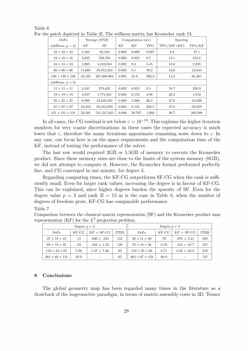
Table 6For the patch depicted in Table 2f. The stiffness matrix has Kronecker rank 13.

DoFs Storage (NNZ) Computation (sec) Speedup

(stiffness, p = 2) KF SF KF KP TPG TPG/(KF+KP) TPG/KF

10× 10× 10 1,585 85,184 0.002 0.008 0.087 8.4 47.1

18× 18× 18 3,025 592,704 0.002 0.055 0.7 12.1 315.8

34× 34× 34 5,905 4,410,944 0.002 0.4 5.45 13.6 2,235

66× 66× 66 11,665 34,012,224 0.003 3.1 39.2 12.6 12,544

130× 130× 130 23,185 267,089,984 0.005 21.6 306.3 14.2 65,461

(stiffness, p = 3)

11× 11× 11 2,341 274,625 0.002 0.025 0.5 18.7 250.9

19× 19× 19 4,357 1,771,561 0.002 0.153 4.08 26.2 1,812

35× 35× 35 8,389 12,649,337 0.003 1.086 29.4 27.0 10,596

67× 67× 67 16,453 95,443,993 0.004 8.142 226.5 27.8 58,659

131× 131× 131 32,581 741,217,625 0.006 58.707 1,802 30.7 289,588

In all cases, the CG residual is set below ε = 10−10. This explains the higher iterationnumbers for very coarse discretizations: in these cases the expected accuracy is muchlower that ε, therefore the many iterations appoximate remaining noise down to ε. Inany case, our focus here is on the space requirements and the computation time of theKF, instead of testing the performance of the solver.

The last row would required 2GB or 5.5GB of memory to execute the Kroneckerproduct. Since these memory sizes are close to the limits of the system memory (6GB),we did not attempt to compute it. However, the Kronecker format performed perfectlyfine, and CG converged in one minute, for degree 3.

Regarding computing times, the KF-CG outperforms SF-CG when the rank is suffi-ciently small. Even for larger rank values, increasing the degree is in favour of KF-CG.This can be explained, since higher degrees burden the sparsity of SF. Even for thedegree value p = 3 and rank R = 13 as is the case in Table 8, when the number ofdegrees of freedom grow, KF-CG has comparable performance.

Table 7Comparison between the classical matrix representation (SF) and the Kronecker product sumrepresentation (KF) for the L2 projection problem.

Degree p = 2

DoFs KF-CG KP + SF-CG ITER

37× 10× 19 .15 .026 + .245 155

69× 18× 35 .82 .192 + 1.33 126

133× 34× 67 5.88 1.47 + 7.48 93

261× 66× 131 32.9 - 65

Degree p = 3

DoFs KF-CG KP + SF-CG ITER

38× 11× 20 .70 .076 + 2.31 505

70× 19× 36 3.19 .545 + 10.7 357

134× 35× 68 6.71 4.22 + 49.3 219

262× 67× 132 68.9 - 121

8 Conclusions

The global geometry map has been regarded many times in the literature as adrawback of the isogeometric paradigm, in terms of matrix assembly costs in 3D. Tensor

28

Table 8Comparison between the classical matrix representation (SF) and the Kronecker product sumrepresentation (KF) for the solution of the isogeometric Laplacian problem.

Degree p = 2

DoFs KF-CG KP + SF-CG ITER

10× 10× 10 .0208 .0084 + .0048 59

18× 18× 18 .1854 .0557 + .0714 78

34× 34× 34 1.920 .3766 + .9012 108

66× 66× 66 33.94 3.198 + 13.90 201

Degree p = 3

DoFs KF-CG KP + SF-CG ITER

11× 11× 11 .078 .022+.035 137

19× 19× 19 .494 .141+.396 144

35× 35× 35 4.12 1.01+2.95 126

67× 67× 67 40.35 9.51+32.32 168

decomposition methods transform this “curse of dimensionality” into a “blessing” forthe efficient implementation of isogeometric analysis. Indeed, both memory requirementsand computation times are drastically reduced, compared to the typical local approachinspired by finite element methods.

Several further improvements can be considered. For example, in our experimentswe used a simple ALS iteration combined with a greedy strategy for canonical tensordecomposition. The rank values obtained by this algorithm are known to be subopti-mal. The reason is that this optimization procedure may converge to local minimum,due to the choice of initial values. More sophisticated methods exist, for instance onecan enhance the algorithm with line search approached to escape from local minima.Nevertheless the obtained suboptimal rank values provide high efficiency gains in theassembly procedure.

An interesting possibility is to use the Kronecker format as the basic matrix format.This has a two-fold advantage, since not only it reduces drastically the matrix generationtimings, but also the memory requirements reduce exponentially. In practice, this mem-ory reduction allows to compute problems of several billions degrees of freedom withoutthe need of a super-computer with terrabytes of memory. It can also be used for keepingthe communication costs low in a distributed memory parallel environment.

Finally, we note that typical volume parameterization such as Gordon-Coon’s vol-umes or swept volumes [1] are expected to have low rank values and are favorable forour algorithm.

Acknowledgements

This research was supported by the National Research Network “Geometry + Simula-tion” (NFN S117, 2012–2016), funded by the Austrian Science Fund (FWF).

References

[1] M. Aigner, C. Heinrich, B. Juttler, E. Pilgerstorfer, B. Simeon, and A. V. Vuong.Mathematics of Surfaces XIII, chapter Swept Volume Parameterization for IsogeometricAnalysis, pages 19–44. Springer Berlin Heidelberg, 2009.

[2] P. Antolin, A. Buffa, F. Calabro, M. Martinelli, and G. Sangalli. Efficient matrixcomputation for tensor-product isogeometric analysis: The use of sum factorization. Comp.Meth. Appl. Mech. Engrg., 285:817–828, 2015.

29

[3] L. B. ao da Veiga, C. Lovadina, and A. Reali. Avoiding shear locking for the timoshenkobeam problem via isogeometric collocation methods. Computer Methods in AppliedMechanics and Engineering, 241244:38 – 51, 2012.

[4] F. Auricchio, L. B. ao da Veiga, J. Kiendl, C. Lovadina, and A. Reali. Locking-freeisogeometric collocation methods for spatial timoshenko rods. Computer Methods inApplied Mechanics and Engineering, 263:113 – 126, 2013.

[5] F. Auricchio, L. Beirao da Veiga, T. J. R. Hughes, A. Reali, and G. Sangalli. Isogeometriccollocation methods. Mathematical Models and Methods in Applied Sciences, 20(11):2075–2107, 2010.

[6] F. Auricchio, F. Calabro, T. Hughes, A. Reali, and G. Sangalli. A simple algorithm forobtaining nearly optimal quadrature rules for NURBS-based isogeometric analysis. Comp.Meth. Appl. Mech. Engrg., 249-252:15–27, 2012.

[7] M. Barton and V. M. Calo. Optimal quadrature rules for odd-degree spline spaces and theirapplication to tensor-product-based isogeometric analysis. Computer Methods in AppliedMechanics and Engineering, 305:217 – 240, 2016.

[8] P. Benner, R.-C. Li, and N. Truhar. On the ADI method for Sylvester equations. Journalof Computational and Applied Mathematics, 233(4):1035–1045, 2009.

[9] D. Braess. Finite Elements: Theory, fast solvers and applications in solid mechanics, thirdedition. Cambridge University Press, 3 edition, 2007.

[10] M. Brand. Fast low-rank modifications of the thin singular value decomposition. LinearAlgebra and its Applications, 415(1):20 – 30, 2006. Special Issue on Large Scale Linear andNonlinear Eigenvalue Problems.

[11] S. Brenner and L. Scott. The Mathematical Theory of Finite Element Methods. Springer-Verlag, 2002.

[12] F. Calabro, G. Sangalli, and M. Tani. Fast formation of isogeometric Galerkin matricesby weighted quadrature. arXiv preprint arXiv:1605.01238, 2016.

[13] P. G. Ciarlet. Finite Element Method for Elliptic Problems. Society for Industrial andApplied Mathematics, Philadelphia, PA, USA, 2002.

[14] N. Collier, D. Pardo, L. Dalcin, M. Paszynski, and V. Calo. The cost of continuity: Astudy of the performance of isogeometric finite elements using direct solvers. ComputerMethods in Applied Mechanics and Engineering, 213216:353 – 361, 2012.

[15] J. A. Cottrell, T. J. R. Hughes, and Y. Bazilevs. Isogeometric Analysis: Toward Integrationof CAD and FEA. John Wiley & Sons, Chichester, England, 2009.

[16] C. de Boor. Efficient computer manipulation of tensor products. ACM Trans. Math.Softw., 5(2):173–182, June 1979.

[17] L. de Lathauwer, B. de Moor, and J. Vandewalle. A multilinear singular valuedecomposition. SIAM J. Matrix Anal. Appl., 21:1253–1278, 2000.

[18] L. de Lathauwer, B. de Moor, and J. Vandewalle. On best rank-1 and rank-(R1, R2, ..., RN )approximation of high-order tensors. SIAM J. Matrix Anal. Appl., 21:1324–1342, 2000.

30

[19] P. Dreesen, M. Ishteva, and J. Schoukens. Decoupling multivariate polynomials usingfirst-order information and tensor decompositions. SIAM Journal on Matrix Analysis andApplications, 36(2):864–879, 2015.

[20] G. Farin. Curves and surfaces for CAGD: a practical guide. Morgan Kaufmann PublishersInc., San Francisco, CA, USA, 2002.

[21] L. Gao and V. M. Calo. Fast isogeometric solvers for explicit dynamics. Comp. MethodsAppl. Mech. Engrg., 274(0):19 – 41, 2014.

[22] L. Gao and V. M. Calo. Preconditioners based on the alternating-direction-implicitalgorithm for the 2d steady-state diffusion equation with orthotropic heterogeneouscoefficients. Journal of Computational and Applied Mathematics, 273(0):274 – 295, 2015.

[23] C. Giannelli, B. Juettler, S. K. Kleiss, A. Mantzaflaris, B. Simeon, and J. Speh. THB-splines: An effective mathematical technology for adaptive refinement in geometric designand isogeometric analysis. Computer Methods in Applied Mechanics and Engineering,299:337 – 365, 2016.

[24] C. Giannelli, B. Juttler, and H. Speleers. THB–splines: The truncated basis for hierarchicalsplines. Computer Aided Geometric Design, 29:485–498, 2012.

[25] H. Gomez, A. Reali, and G. Sangalli. Accurate, efficient, and (iso)geometrically flexiblecollocation methods for phase-field models. Journal of Computational Physics, 262(0):153– 171, 2014.

[26] L. Grasedyck, D. Kressner, and C. Tobler. A literature survey of low-rank tensorapproximation techniques. GAMM-Mitteilungen, 36(1):53–78, 2013.

[27] W. Hackbusch. Tensor spaces and numerical tensor calculus. Springer, Berlin, 2012.

[28] W. Hackbusch, B. N. Khoromskij, and E. E. Tyrtyshnikov. Hierarchical kronecker tensor-product approximations. Journal of Numerical Mathematics, 13(2):119–156, 2005.

[29] N. Halko, P. G. Martinsson, and J. A. Tropp. Finding structure with randomness:Probabilistic algorithms for constructing approximate matrix decompositions. SIAM Rev.,53(2):217–288, May 2011.

[30] R. R. Hiemstra, F. Calabro, D. Schillinger, and T. J. Hughes. Optimal and reducedquadrature rules for tensor product and hierarchically refined splines in isogeometricanalysis. ICES REPORT 16-11, 2016.

[31] M. Hillman, J. Chen, and Y. Bazilevs. Variationally consistent domain integration forisogeometric analysis. Comp. Meth. Appl. Mech. Engrg., 284:521–540, 2015.

[32] F. L. Hitchcock. The expression of a tensor or a polyadic as a sum of products. J. Math.Phys, 6(1):164–189, 1927.

[33] T. Hughes, J. Cottrell, and Y. Bazilevs. Isogeometric analysis: CAD, finite elements,NURBS, exact geometry and mesh refinement. Comp. Meth. Appl. Mech. Engrg., 194(39–41):4135–4195, 2005.

[34] T. Hughes, A. Reali, and G. Sangalli. Efficient quadrature for NURBS-based isogeometricanalysis. Comp. Meth. Appl. Mech. Engrg., 199(5 – 8):301–313, 2010.

31

[35] B. Juettler, U. Langer, A. Mantzaflaris, S. Moore, and W. Zulehner. Geometry +simulation modules: Implementing isogeometric analysis. Proc. Appl. Math. Mech.,14(1):961–962, 2014. Special Issue: 85th Annual Meeting of the Int. Assoc. of Appl. Math.and Mech. (GAMM), Erlangen 2014.

[36] V. Khoromskaia and B. N. Khoromskij. Tensor numerical methods in quantumchemistry: from Hartree-Fock to excitation energies. Phys. Chem. Chem. Phys.,DOI:10.1039/c5cp01215e, 2015.

[37] B. N. Khoromskij. O(d log n)–Quantics approximation of N–d tensors in high-dimensionalnumerical modeling. Constr. Appr., 34(2):257–280, 2011.

[38] B. N. Khoromskij. Tensor-structured numerical methods in scientific computing: surveyon recent advances. Chemometr. Intell. Lab. Syst., 110(1):1–19, 2012.

[39] B. N. Khoromskij and V. Khoromskaia. Low rank Tucker-type tensor approximation toclassical potentials. Central European journal of mathematics, 5(3):523–550, 2007.

[40] B. N. Khoromskij and V. Khoromskaia. Multigrid accelerated tensor approximation offunction related multidimensional arrays. SIAM J. Sci. Comput., 31(4):3002–3026, 2009.

[41] T. Kolda and B. Bader. Tensor decompositions and applications. SIAM Review, 51/3:455–500, 2009.

[42] M. Los, M. Wozniak, M. Paszynski, L. Dalcin, and V. Calo. Dynamics with matricespossessing kronecker product structure. Procedia Computer Science, 51:286 – 295, 2015.

[43] A. Mantzaflaris, B. Juettler, B. Khoromskij, and U. Langer. Matrix generation inisogeometric analysis by low rank tensor approximation. In J.-D. Boissonnat, A. Cohen,O. Gibaru, C. Gout, T. Lyche, M.-L. Mazure, and L. L. Schumaker, editors, Curves andSurfaces, volume 9213 of LNCS, pages 321–340. Springer, 2015.

[44] A. Mantzaflaris and B. Juttler. Integration by interpolation and look-up for Galerkin-based isogeometric analysis. Comp. Methods Appl. Mech. Engrg., 284:373 – 400, 2015.Isogeometric Analysis Special Issue.

[45] I. V. Oseledets. Tensor-train decomposition. SIAM J. Sci. Comput., 33(5):2295–2317,2011.

[46] G. Sangalli and M. Tani. Isogeometric preconditioners based on fast solvers for theSylvester equation, 2016.

[47] D. Schillinger, L. Dede, M. Scott, J. Evans, M. Borden, E. Rank, and T. Hughes.An isogeometric design-through-analysis methodology based on adaptive hierarchicalrefinement of NURBS, immersed boundary methods, and t-spline CAD surfaces. Comp.Meth. Appl. Mech. Engrg., 249 – 252:116 – 150, 2012.

[48] D. Schillinger, J. Evans, A. Reali, M. Scott, and T. Hughes. Isogeometric collocation:Cost comparison with Galerkin methods and extension to adaptive hierarchical NURBSdiscretizations. Comp. Meth. Appl. Mech. Engrg., 267:170–232, 2013.

[49] D. Schillinger, S. Hossain, and T. Hughes. Reduced Bezier element quadrature rules forquadratic and cubic splines in isogeometric analysis. Comp. Meth. Appl. Mech. Engrg.,277(0):1 – 45, 2014.

32

[50] L. Schumaker. Spline Functions: Basic Theory. Cambridge University Press, 3 edition,2007.

[51] L. R. Tucker. Some mathematical notes on three-mode factor analysis. Psychometrika,31:279–311, 1966.

[52] C. F. van Loan and N. Pitsianis. Approximation with Kronecker products. In Linearalgebra for large scale and real-time applications (Leuven, 1992), volume 232 of NATOAdv. Sci. Inst. Ser. E Appl. Sci., pages 293–314. Dordrecht, 1993.

33