Low volatility sector-based portfolios: a South African case · Low volatility sector-based...

Volume 32 (1), pp. 55–78

http://orion.journals.ac.za

ORiONISSN 0259–191X (print)ISSN 2224–0004 (online)

c©2016

Low volatility sector-based portfolios:a South African case

OS Oladele∗ D Bradfield†

Received: 22 June 2015; Revised: 29 February 2016; Accepted: 2 March 2016

Abstract

Portfolios and indices that have been specifically constructed to have low risk attributeshave received increasing interest in the recent international literature. It has been foundthat portfolios constructed by targeting low risk assets have predominantly outperformedportfolios constructed to have higher risks. This anomaly has led to renewed interest inconstructing low volatility portfolios by practitioners. This study analyses a variety of lowvolatility portfolio construction methodologies using sectors as building blocks in the SouthAfrican environment. The empirical results from back-testing these portfolios show significantpromise in the South African setting when compared with a market capitalization-weightedbenchmark. In the empirical analysis in the South African environment two techniques standout as being superior low volatility construction techniques amongst the seven techniquesassessed. Furthermore, the low volatility portfolios are blended with typical general equityportfolios (using the Shareholder-Weighted Index (SWIX) as a proxy). It was found that theseblended portfolios have useful features which lead to enhanced performance and therefore canserve as effective portfolio strategies.

Key words: Low volatility portfolios, Minimum Variance (MVP), Low Volatility Single Index Model

(SIM), Equal Risk Contribution (ERC), Naıve Risk Parity (NRP), Maximum Diversification (MDP), Equal

Weighting (EW), Covariance Bi-plot.

1 Introduction

Support for the low volatility anomaly stems from the criticism of the Capital Asset Pric-ing Model (CAPM), which states that assets with high systematic risk are expected toearn higher expected returns, while low beta assets are expected to have lower returns[33, 40]. However, evidence of a low volatility anomaly was first discovered by Black [3]who demonstrated empirically that the security market line is flatter than predicted by the

∗Department of Statistical Sciences, University of Cape Town, 7700 Rondebosch, South Africa†Corresponding author: Department of Statistical Sciences, University of Cape Town, 7700 Rondebosch,

South Africa, email: [email protected]

http://dx.doi.org/10.5784/32-1-541

55

http://orion.journals.ac.za

[email protected]

http://dx.doi.org/10.5784/32-1-541

56 OS Oladele & D Bradfield

CAPM. Black pointed out that when investors are restricted from using leverage or bor-rowing, they tend to buy high-risk assets thereby leaving the low-risk assets under-priced.This evidence has led to an increasing interest in the formation of low volatility portfoliosthat not only have lower risks out-of-sample than market-cap-weighted portfolios, but alsohave higher risk-adjusted returns out-of-sample than market-cap-weighted portfolios.

Recently, Baker et al. [2] gave some behavioral reasons as to why some investors maycreate an excess demand for high-risk stocks that have historically underperformed. Theyalso argued why investors might typically avoid buying low-risk stocks. The reasons Bakeret al. [2] put forward were:

• Investors preference for lottery-like payoffs; implying that investors accept a lowprobability of receiving a large windfall.

• Representativeness bias, which suggests that investors prefer high-risk stocks thatcontain a lot of news. Hence, they buy the stock at a high price, which in turn lowersthe return of the stock.

• Portfolio managers are required to beat a specific benchmark and to minimize thetracking error relative to that benchmark. Hence, they are averse to investing in lowbeta stocks, because of their high tracking error relative to the benchmark.

The primary objective of this study is to assess the performance of low volatility portfoliosconstructed from indices relative to the market capitalization-weighted indices using theFTSE/JSE sectors. The use of sectors for portfolios was motivated by Leclerc et al. [25],who created industry-based weighting schemes in the U.S. markets. Leclerc et al. [25]named their industry-based weighting scheme Alternative Equity Indices (AEI’s) whichwere designed as alternatives to market capitalization-weighted portfolios. Leclerc et al.[25] gave the following reasons for using sectors to construct low volatility portfolios ratherthan stocks: Firstly, constructing portfolios based on sectors help in overcoming the curseof dimensionality as explained by Michaud [35]. That is, the number of parameters toestimate is reduced. Secondly, even though some stock-constituent AEI’s may outperformthe sector-based AEI’s before transaction cost, the sector-based AEI’s are still considereda reasonable choice in terms of capacity, transparency, liquidity and resultant transactioncosts. Lastly, sector tilts are important in explaining constituent-based stocks outperfor-mance over the market capitalization indices.

In brief, the study involves the assessment of a range of sector-based low volatility tech-niques found in recent literature for constructing portfolios. These portfolios are rebalancedmonthly using a 36 months rolling window to estimate the covariance matrix. Additionally,the Ledoit & Wolf [26] shrinkage covariance estimator is used to reduce the effect of errorsin the sample covariance matrix. The performances of the sector-based low volatility port-folios are then compared with the ALSI (the market capitalization-weighted benchmark).

The main contributions of this article are: Firstly, different portfolio construction tech-niques for forming the low volatility portfolios (based on sectors) are demonstrated andassessed in the South African equity market. Secondly, the Ledoit & Wolf [26] covarianceshrinkage estimator is utilised in the portfolio construction process of the portfolios. Fi-nally, sector-based low volatility portfolios are blended (with the Shareholder-WeightedIndex (SWIX)) in order to establish their usefulness as a combined portfolio strategy.

Low volatility sector-based portfolios: a South African case 57

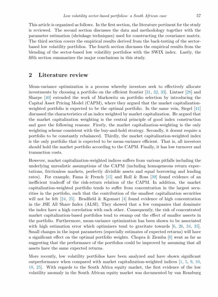
This article is organized as follows. In the first section, the literature pertinent for the studyis reviewed. The second section discusses the data and methodology together with theparameter estimation (shrinkage techniques) used for constructing the covariance matrix.The third section covers the empirical results derived from the back-testing of the sector-based low volatility portfolios. The fourth section discusses the empirical results from theblending of the sector-based low volatility portfolios with the SWIX index. Lastly, thefifth section summarizes the major conclusions in this study.

2 Literature review

Mean-variance optimization is a process whereby investors seek to effectively allocateinvestments by choosing a portfolio on the efficient frontier [31, 32, 33]. Lintner [28] andSharpe [40] extended the work of Markowitz on portfolio selection by introducing theCapital Asset Pricing Model (CAPM), where they argued that the market capitalization-weighted portfolio is expected to be the optimal portfolio. In the same vein, Siegel [41]discussed the characteristics of an index weighted by market capitalization. He argued thatthe market capitalization weighting is the central principle of good index constructionand gave the following reasons: Firstly, the market capitalization-weighting is the onlyweighting scheme consistent with the buy-and-hold strategy. Secondly, it doesnt require aportfolio to be constantly rebalanced. Thirdly, the market capitalization-weighted indexis the only portfolio that is expected to be mean-variance efficient. That is, all investorsshould hold the market portfolio according to the CAPM. Finally, it has low turnover andtransaction costs.

However, market capitalization-weighted indices suffers from various pitfalls including theunderlying unrealistic assumptions of the CAPM (including homogeneous return expec-tations, frictionless markets, perfectly divisible assets and equal borrowing and lendingrates). For example, Fama & French [15] and Roll & Ross [39] found evidence of aninefficient tradeoff of the risk-return relation of the CAPM. In addition, the marketcapitalization-weighted portfolio tends to suffer from concentration in the largest secu-rities in the portfolio, such that the contribution of the smallest capitalization securitieswill not be felt [24, 25]. Bradfield & Kgomari [4] found evidence of high concentrationin the JSE All Share Index (ALSI). They showed that a few companies that dominatethe index have a high correlation with each other. Consequently, the risk of concentratedmarket capitalization-based portfolios tend to swamp out the effect of smaller asserts inthe portfolio. Furthermore, mean-variance optimization has been shown to be associatedwith high estimation error which optimizers tend to gravitate towards [6, 26, 34, 35].Small changes in the input parameters (especially estimates of expected returns) will havea significant effect on the optimal portfolio weights. Chopra & Ziemba [6] went as far assuggesting that the performance of the portfolios could be improved by assuming that allassets have the same expected returns.

More recently, low volatility portfolios have been analyzed and have shown significantoutperformance when compared with market capitalization-weighted indices [1, 5, 9, 10,18, 25]. With regards to the South Africa equity market, the first evidence of the lowvolatility anomaly in the South African equity market was documented by van Rensburg


& Robertson [43], where it was found that the beta of a stock is negatively related to itsreturn. Recently, Kruger et al. [23] also found similar evidence of the low volatility anomalyusing a more refined beta estimate. Furthermore, the performance of a variety of lowvolatility portfolios has also been assessed in out-of-period settings [21, 37]. Khuzwayo [21]for example found strong evidence in support of the low volatility anomaly in South Africa(using the Top 100 JSE stocks from 2001-2011). Khuzwayo showed that the low volatilityportfolios constructed had a lower drawdown and also outperformed the market portfolio.Panulo [37] constructed risk parity portfolios and other risk-based portfolios which showedsignificant outperformance compared with the market capitalization-weighted index (AllShare Index).

The sector-based low volatility portfolios examined in this article have been sourced fromrecent literature and they are: the Equally-Weighted (EW), the equal-weighted Low Beta(Lowbeta), the Minimum Variance Portfolio (MVP), the low Volatility Single Index Model(SIM), the Equal Risk Contribution (ERC), Naıve Risk Parity (NRP), and the MaximumDiversification Portfolio (MDP). Table 1 contains a summarised description of these port-folios as found in the literature.

Techniques Targets Required parameter Formula

EW [14] Maximum weights No risk or returndiversification parameter

wi = 1/N

Lowbeta [25] Low beta assets Beta wi = 1/NLMVP [10, 18] Low volatility assets Covariance matrix

and low correlationw∗ = min

∑Ni=1

∑Nj=1 wiwjσij

SIM [11] Low beta and low Beta and idiosyn-volatility assets cratic variance

wi =σ2mv

σ2i

(1− βi

βL

)ERC[29] Maximum risk Volatility and

diversification correlationmin

∑Ni=1

∑Nj=1

(wi

∂σp∂wi− wj

∂σp∂wj

)2NRP [29, 38] Assets with lower Volatility

volatilities than otherswi =

1/σi∑Ni=1

1/σi

MDP [7, 8] Low correlation with Volatility andother assets correlation

w∗ = arg max wiσσp

Table 1: A summary of the low volatility portfolios.

To be consistent with developments in the mean-variance framework of Markowitz [31], itis noted that all of the authors mentioned in Table 1 were concerned with low standarddeviation or variance of return, rather than some other measure of risk, for example semi-variance (downside risk). It is pointed out that portfolios targeting semi-variance shouldbe the same as those targeting variance if the underlying distributions are symmetrical.Whilst low semi-variance may be an interesting metric to target, it is left to directionsfor further research and we thus focus on the standard deviation of returns instead inthis article. As standard deviations are couched in the same units as returns, refer toannualised risk as being the annualised standard deviation of returns.

2.1 The different low volatility construction methodologies

In this section, the construction of the sector-based low volatility portfolios (as summarizedin Table 1) is briefly discussed and their performance as reported in the literature isreviewed.


2.1.1 The naıve equally-weighted portfolio

The first methodology, the naıve equally-weighted portfolio (EW), assigns an equal weightto each sector. For a universe of N sectors, the EW portfolio assigns weights equally andis given by

wi = 1/N, (1)

where wi are the portfolio weights of sector i with i = 1, 2, . . . , N .

The EW technique in essence assumes that the risk and return cannot be forecasted [27].This strategy thus helps to reduce the impact of concentration of risk by having equalweights. Thus, with the EW strategy investors are equally exposed to the smallest sectorsas well as the largest sectors in the portfolio.

DeMiguel et al. [14] analyzed 7 empirical datasets of monthly returns using the U.S. small-,mid- and large-cap indices and compared the out-of-sample performance of 14 differentmodels. They found that the benefits of optimal portfolio strategies are more than offsetby estimation errors. Consequently, none of the 14 different models performed better thanthe naıve equal weighting strategy.

2.1.2 The equal-weighted low beta portfolio

The equal-weighted low beta portfolio (Lowbeta) is formed by equal weighting those sectorswith the lowest 20% of betas. It is given by

wi = 1/NL, (2)

where NL is the number of sectors in the Lowbeta portfolio.

The intuition for using the Lowbeta portfolio for the sectors was motivated by the worksof Black [3] and Haugen & Heins [19] who showed that low-beta stocks have historicallyoutperformed high-beta stocks. In the same vein, Frazzini & Lasse [16] and Frazzini &Pedersen [17] also found outperformance of low-beta stocks over the high-beta stocks intheir betting versus beta factor strategy. Recently, Khuzwayo [21] computed low-betaversus high-beta stocks using the Top 100 JSE shares over the period 2001 to 2011 andcompared their performance with the All Share Index (ALSI). He found that during thesample period, the low-beta portfolios outperformed both high-beta portfolios and theALSI.

2.1.3 The minimum variance portfolio

The Minimum Variance Portfolio (MVP) is the portfolio located on the left-most positionof the efficient frontier, and is made up of the least volatile joint collection of assets [10, 18].The objective function of the MVP is to minimize total portfolio risk and is given by

w∗ = minN∑i=1

N∑j=1

wiwjσij , (3)

where σij is the covariance between the returns of sectors i and j.


The MVP portfolio is considered more robust than the optimal portfolio (in mean-variancespace as defined by Markowitz [31]) because of the optimal portfolios sensitivity to inputsin the forecast return vector and the covariance matrix [6, 26, 34, 35]. Clarke et al. [10]constructed portfolios using the MVP technique and found higher realized average returnsand lower risks than the market return by using shrinkage methods1 applied to the samplecovariance matrix using large-cap U.S. stocks over the periods 1968 to 2009. Jagannathan& Ma [20] also constructed MVPs by imposing weight constraints and found them equiva-lent to using a shrinkage estimator on the variance-covariance matrix. Kritzman et al. [22]found higher Sharpe ratios in their MVP techniques constructed relative to the EW andmarket capitalization-weighted indices. Similarly, Haugen & Baker [18] also showed thatthe MVP technique outperformed the Wilshire 5000 at a lower risk between the periods1972 to 1989.

2.1.4 The low volatility single index model

The low Volatility Single Index Model (SIM) was proposed by Clarke et al. [11]. Theyderived an analytic solutions for the positive weights (long-only portfolios) using Sharpessingle-index model [40] for their minimum variance portfolio construction. The SIM tech-nique assumes that the only common source of risk is a single factor (the market portfolio).Using the decomposition of an assets risk into the idiosyncratic risk and the systematicrisk, [11] derived the SIM weights as

wi =σ2mv

σ2ei

(1− βi

βL

)for βi < βL else wi = 0, (4)

where βL is the beta-bound (threshold beta) of the long-only assets, βi is the beta of theasset to the common factor (the market), σ2

mv is the ex-ante variance of the long-only SIMminimum variance portfolio, and σ2

ei is the ex-ante idiosyncratic variance for asset i.

The equation above suggests that the portfolio weights are highly dependent on the betasand idiosyncratic risk. However, Clarke et al. [11] argued that the idiosyncratic risk will notdrive the asset out of the solution. In addition, the equation also targets those assets withbetas that are lower than the long-only threshold beta (βL). The formula for calculatingβL is given by

βL =

1σ2m

+∑

βi<βL

β2i

σ2ei∑

βi<βLβiσ2ei

, (5)

where σ2m is the market variance.

The method for calculating βL is to first sort the betas of sectors in ascending order, thenthe beta of each sector is compared with the cumulative summation term until the betaof the sector exceeds the cumulative right-hand-side (RHS) value yielding the requiredthreshold beta.

Clarke et al. [11] compared SIM portfolios, with other low volatility portfolios using 1 000U.S. stocks over the period 1968 to 2012 and then compared these with the market cap-

1They used both Asymptotic Principal Component by Connor & Korajczyk [13] and Bayesian shrinkageestimation of Ledoit & Wolf [26].


italization weighted portfolio. They found that the SIM portfolio posted the lowest riskand the highest Sharpe ratios. Additionally in South Africa Khuzwayo [21] found higherSharpe ratios for the SIM portfolios when compared with the performance of the MVP,MDP, EW portfolios as well as the ALSI 100 during the periods 2008 to 2011.

2.1.5 The equal risk contribution portfolio

The Equal Risk Contribution portfolio (ERC) aims to allocate risk equally among sectors.Qian [38] for example found that equities contribute over 90% of the risk of a 60/40(equity/bond) portfolio resulting in a large concentration of risk in the portfolio. TheERC portfolios instead allocates weight to sectors by their contribution to risk and thustakes into account the correlation between the sectors in a portfolio. As a result, theERC portfolio targets risk diversification by focusing on sectors with low volatility andlow correlation with other assets [27, 29]. The ERC portfolio derived by Maillard et al.[29] computes the portfolio weights using a sequential quadratic programming as

w∗ = arg minN∑i=1

N∑j=1

(wi∂MCRp(w)

∂w− wj

∂MCRp(w)

∂w

)2

, (6)

where wi∂MCRp(w)

∂w is the risk contribution to the portfolio (the weights of the sectors inthe portfolio multiplied by the marginal risk contribution to the portfolio).

From equation (6), the ERC portfolio will allocate higher weight to sectors that have lowcorrelation and volatility with other sectors. Maillard et al. [29, 30] compared the EW,ERC, MDP and MVP using equity U.S. sectors. They found that all strategies, exceptthe EW, outperformed the market capitalization portfolio with a lower volatility. Theyalso showed that the volatility of the ERC portfolio is located between the EW portfolioand the MVP.

2.1.6 The naıve risk parity portfolio

In contrast to the ERC technique, the Naıve Risk Parity (NRP) technique, assumes that allsectors have the same pair-wise correlations. The optimal portfolio weights are computedanalytically and can be expressed as

wi =1/σi∑Ni=1 1/σi

, (7)

where σi is the volatility of sector i. From equation (7), it follows that sectors that aremore risky than others will receive a lower weight in the portfolio.

2.1.7 The maximum diversification portfolio

Finally, the Maximum Diversification Portfolio (MDP) technique is examined, which isconstructed to maximize a diversification ratio as derived by Choueifaty & Coignard [7].


The diversification ratio is defined as the ratio of the weighted average of volatility to theportfolio volatility and is given by

w∗ = arg max

∑wiσiσp

, (8)

where σi is the volatility of an individual asset and σp is the portfolio volatility.

From the equation above, the MDP technique will rather allocate weight based on theasset’s correlation with the portfolio. This suggests that the MDP portfolio will invest insectors that are less correlated to the portfolio, which will in turn, increases the diversi-fication ratio. Choueifaty & Coignard [7] investigated the performance of the MDP, withthe EW and the MVP portfolios using constituents stocks from S&P 500 and Dow JonesEURO STOXX Large Cap indices over the period 1992–2007. They showed that the MDPproduced the highest return.

2.2 Covariance matrix estimation

At the heart of the sector-based low volatility portfolio strategies is the estimation of thecovariance matrix. The covariance matrix is an important input source that plays a centralrole in producing the optimal portfolio weights. Thus, small changes in input assumptionsof the covariance matrix may imply large changes in the portfolio weights. Michaud [35]proposed using resampling methods to estimate the mean and covariance terms. Ledoit &Wolf [26] derived a shrinkage transformation on the sample covariance matrix and appliedit to monthly U.S. stock data. They showed that the shrinkage estimator reduces thetracking error relative to the benchmark index. Clarke et al. [10] used both the Ledoit& Wolf [26] Bayesian shrinkage estimator (Constant Correlation Model) and the Connor& Korajczyk [13] asymptotic principal component method in implementing their mini-mum variance optimization. They found that the Bayesian shrinkage estimator producesa better result than the asymptotic principal component approach. In the South Africanenvironment Munro & Bradfield [36] compared the performance of different shrinkage esti-mators (the Constant Correlation Shrinkage Model, the Single Index Model, the PrincipalComponent Model, and the Average Covariance Model). They found that the ConstantCorrelation Model produced the lowest risk when using the MVP framework.

On the basis of the findings of Munro & Bradfield [36], the Ledoit & Wolf [26] Bayesianshrinkage estimator was adopted to estimate the covariance matrix in the ensuing empiricalstudy. The Ledoit & Wolf [26] Bayesian shrinkage technique involves finding a compro-mise between the sample covariance matrix S and a shrinkage target (highly structuredestimator F ). They found a convex linear combination of both S and F as

Ω∗ = µF + (1− µ)S, (9)

where µ is a shrinkage constant between 0 and 1. In the Ledoit & Wolf [26] case, the highlystructured estimator used as the shrinkage target is the Constant Correlation Model.


3 Data and methodology

The sample data used for analysis cover the 9 FTSE/JSE sectors from January 2003 toDecember 2013, which were collected from Datastream.

3.1 Description of the data

The 9 FTSE/JSE sectors in the data are the Oil and Gas, Basic Materials, ConsumerGoods, Health Care, Consumer Services, Telecoms, Financials, Industrials, and the Tech-nology sectors. The monthly total return indices were adjusted for all corporate actions.Table 2 describes the annualised return, annualised risk, Sharpe ratio (assuming a riskfree rate of 8.43%), and drawdown2 for the FTSE/JSE sectors.

FTSE/JSE sectors Annualised Annualised Annualised Drawdownreturn risk Sharpe

Oil and Gas 16% 25% 0.27 44%Basic Materials 10% 25% 0.05 53%Consumer Goods 24% 21% 0.68 38%Health Care 26% 19% 0.88 37%Consumer Services 29% 18% 1.05 30%Telecoms 28% 23% 0.77 39%Financials 18% 17% 0.5 46%Technology 24% 28% 0.49 48%

Table 2: Descriptive statistics for the 9 FTSE/JSE sectors from January 2003 to December

2013.

Figure 1 shows the correlation matrix between the 9 sectors. From Figure 1, it is evidentthat there is a high correlation between the Oil and Gas, Basic Materials, and ConsumerGoods and the ALSI.

3.2 Methodology

The low volatility portfolios are rebalanced monthly over the period 2003–2013 for thesectors, assuming a trading cost of 25 basis points (bps). The general methodology fol-lows the approach of Snopek [42] in the construction of the minimum variance portfolio.Additionally the following constraints are imposed.

• Fully invested constraint in the risky portfolio, that is∑N

i=1wi = 1.

• Long-only constraint (wi ≥ 0).

Figure 2 depicts the methodology for constructing the low volatility portfolios. FromFigure 2, the first covariance estimation period takes is from t0 = January 2003 to t1 =December 2005. The in-sample weights as at December 2005 are then multiplied by theout-of-sample 1 month return i.e. for January 2006, resulting in the portfolio return for

2Drawdown is defined to be the worst cumulative loss that a sector sustained, taken over the wholeperiod of the analysis.


OIL&GAS

value1.0

BASIC MATS

CONSUMER GDS

HEALTH CARE

CONSUMER SVS

TELECOM

FINANCIALS

TECHNOLOGY

INDUSTRIALSALSI

OIL&GAS

BASIC MATS

CONSUMER GDS

HEALTH CARE

CONSUMER SVS

TELECOM

FINANCIALS

TECHNOLOGY

INDUSTRIALS

ALSI

0.80.60.4

Figure 1: Correlation matrix for the FTSE/JSE sectors for January 2003 to December 2013.

that month. The entire process is then rolled forward 1 month, from t′0 = February2003 to t′1 = January 2006. This procedure is rolled forward monthly repeatedly untilthe end of data period is reached, at December 2013. Additionally in the estimationperiod, the low volatility portfolios that will require construction by optimization are theMVP, ERC, and the MDP portfolios. The EW, Lowbeta, NRP, and SIM portfolios do notrequire optimization. Recalculation of the betas is, however, required for constructing boththe Lowbeta and SIM portfolios. The historical betas are estimated using the standardordinary least square estimates of the previous 36 months, where the common marketfactor is the ALSI. For the Lowbeta portfolio, equal weights are assigned to sector betaslower than 50th percentile beta (≤ 50%).

In-Sample period

Out-of-SampleReturn Matrix

In-Sample periodOut-of-SampleReturn Matrix

Figure 2: Methodology for the monthly rebalancing on the FTSE/JSE sectors adapted from

Snopek [42].


4 Empirical performance

Table 3 reports the out-of-sample performance statistics for the low volatility portfoliosafter accounting for rebalancing cost (assumed to be 25bps) at each rebalancing date,from January 2006–December 2013. The Gini Weight measures the average sector weightconcentration while the Gini Risk measures the average sector risk decomposition for thelow volatility portfolios. The Gini index is a measure of dispersion using the Lorenz curve[29]. The Lorenz curve is a graphical representation of the cumulative distribution of thedistribution of wealth in a society, where the statistics of interest may be the income ofa population. Mathematically, the Gini index G is computed as G = 1 − 2

∫ 10 L(x) dx

where L(x) is the Lorenz curve. Applying this concept to the low volatility portfolios, thestatistics of interest become the weights and risk contributions of a portfolio.

Lowbeta SIM MDP NRP ERC EW MVP SWIX ALSI

Annualised Return 23% 21.4% 21.5% 20.6% 20.5% 20.3% 20.1% 16.7% 16.3%Annualised Risk 15% 15.3% 15.7% 14.8% 14.9% 15% 15.4% 15.8% 17.1%Annualised Sharpe 0.86 0.78 0.75 0.74 0.73 0.71 0.69 0.52 0.41Drawdown 31% 33% 37% 32% 32% 31% 37% 36% 41%Beta 0.7 0.69 0.76 0.79 0.8 0.81 0.76 0.89Correlation (ALSI) 0.79 0.79 0.84 0.91 0.92 0.92 0.84Correlation (SWIX) 0.82 0.87 0.97 0.96 0.96 0.94 0.89Information Ratio3 63% 48% 41% 61% 62% 60% 41% 10%No. of Sectors 5 6 7 9 9 9 6 9 9Gini Weight 0.44 0.52 0.63 0.11 0.1 0 0.63 0.55 0.49Gini Risk 0.49 0.51 0.63 0.08 0.06 0.11 0.63 0.4 0.57

Table 3: Out-of-sample performance measures of the low volatility portfolios relative to the

ALSI from January 2006 to December 2013.

The low volatility portfolios are also ranked from the highest Sharpe ratios to the lowestSharpe ratios. Appendix A also depicts the evolution of the sector weights and riskcontribution of each sector over the 2006–2013 test period. In addition, Appendix Bshows the average sector weights and the last known weights of each sector in the lowvolatility portfolios.

From Table 3, it is evident that all of the portfolios outperformed the ALSI in terms oflower risk and higher Sharpe ratios. More salient is the high Sharpe ratio of the Lowbeta(0.86) and the SIM (0.78) portfolios over the period. Furthermore, the portfolios alsoshowed a lower drawdown than the ALSI. The Lowbeta portfolio also posted the lowestdrawdown of 0.31, whereas the MVP and SIM portfolio had the highest drawdown of0.37 amongst the low volatility portfolios. Note that the SIM, and the Lowbeta had ahigh tracking error4 (11%) relative to the ALSI, whereas, the ERC, NRP, MDP, MDS,and EW techniques posted a lower tracking error relative to the ALSI. Interestingly theseportfolios that have been constructed on the basis of in-sample betas have preserved these

3The information ratio of a portfolio is the active premium (portfolio annualised return minus bench-mark annualised returns) divided by the tracking error.

4The tracking error of a portfolio is the standard deviation of the difference between the portfoliosreturns and the benchmark returns.


low beta characteristics out-of-sample (for example the betas of the Lowbeta (0.7), MVP(0.76), and SIM (0.69) techniques were the lowest of all portfolios). As with Maillardet al. [30] Gini statistics are included in Table 3. Regarding the interpretation of theGini statistics, it is noted that the Gini statistic takes on the value of 1 for a perfectlyconcentrated portfolio and 0 for an equally-weighted one. In essence the closer to zero,the less concentrated are the weights (and risk contributions), and the closer to one, themore concentrated the weights and risks contributions are. For the Gini risks, instead ofusing weights, the contribution to portfolio risks is calculated instead (weights of sectorsmultiplied by the marginal risk contribution). Once more the Gini risk for a portfolio isproportional to its risk contribution mapped out by the Lorenz curve.

Furthermore, the Gini Weight, and Gini Risk from Table 3 suggests that:

• The Gini Weight for the ALSI had a weight of 0.49 and Gini Risk of 0.57. BasicMaterials, Financials and Consumer Goods were the dominant sectors in the indexwhile the Technology, Health care, Oil and Gas, Consumer Services and Industrialswere the least dominant sectors (see Figure A.1).

• The Gini Weights for the MVP, and SIM techniques (0.63 and 0.52) were relativelymore concentrated (see Figure A.2 and A.3), with Gini Risks of 0.63 and 0.51 re-spectively. This perhaps is not surprising, given that the minimum variance strategyassigns weights to low beta sectors specifically the Consumer Goods, Health care,Financials and Industrials.

• For the Lowbeta portfolio, the Gini Weight and Gini Risk (0.44 and 0.49) werelowest respectively (less concentrated). The Lowbeta portfolio is dominated by lowbeta sectors, thus over the sample period, Financials, Health care, Consumer goods,Consumer services, and Industrials were mostly included in the equal weight lowbeta portfolio (see Figure A.8).

• The Gini Weights for the EW, ERC and NRP techniques (0, 0.10 and 0.11 respec-tively) have the lowest concentration. For the EW technique, all sectors were givenequal weight (see Figures A.4, A.5 and A.7).

• The Gini Weight for the MDP technique is 0.63, while its respective Gini Risk posted0.63 which also suggests this portfolio is fairly highly concentrated (see Figure A.6).

Figure 3 depicts the out-of-sample cumulative returns of the low volatility portfolios,together with the ALSI and SWIX indices. From Figure 3, one notices that most strategiestend to move in sync with each other. For example the EW, MDP, ERC and NRPtechniques respectively are found to move together to a large degree. Importantly, all lowvolatility portfolios have outperformed the ALSI and the SWIX indices.

Similarly, Figure 4 depicts the risk-return positions of the low volatility portfolios, togetherwith the ALSI and the SWIX indices. From Figure 4, it is evident that the Lowbeta, MVP,SIM, MDP, and the ERC portfolio, posted lower risks but also higher returns over thesample period. This is similar to the results of Clarke et al. [11], Clarke et al. [12], Maillardet al. [29], Choueifaty & Coignard [7], Baker et al. [2], Khuzwayo [21] and Velvadapu [44]who all found that low volatility portfolios have outperformed the market capitalizationportfolios over time.


Figure 3: Out-of-sample cumulative returns of the FTSE/JSE sector-based low volatility port-

folios January 2006–December 2013.

Figure 4: Risk-return plot of the sector-based low volatility portfolios, January 2006–December

2013.

To gain more insight into the performance of the low volatility strategies in various mar-ket regimes, the period is divided into 2 equal sub-periods, each having distinct marketregimes. The first period (1 January 2006 to 31 December 2009) contained the period ofthe financial crises, whilst the second sub-period (1 January 2010 to 31 December 2013)characterised the market recovery period. Table 4 shows the cumulative return of each ofthe strategies (including the ALSI and SWIX) in each sub-period.

In sub-period 1 of Table 4 (characterized by the financial crisis) all the low volatilitystrategies, with the exception of the MVP strategy, outperformed both the ALSI and theSWIX. In the second sub-period (characterized by the market recovery), all of the low-volatility strategies again outperform the ALSI and SWIX benchmarks, suggesting thatthe general outperformance of the low volatility strategies seem to have been consistentacross market regimes.


Return period MVP SIM ERC NRP MDP EW Lowbeta ALSI SWIX

2006–2009 72% 86% 89% 90% 96% 91% 103% 82% 77%2010–2013 327% 302% 269% 268% 274% 256% 280% 178% 198%

Table 4: Out-of-sample cumulative return performance for the 2 sub-periods.

5 Blending of sector-based low volatility portfolios

Having assessed the performance of the low volatility portfolios under the constraint offull investment, one could imagine that active portfolio managers are unlikely to invest alltheir capital in these low volatility portfolios. Active managers typically have an investstyle to generate active returns that they market to clients and are consequently morelikely to want to enhance their risk-return performance by tilting towards low volatilityportfolios, rather than to invest fully in them.

The blended portfolios are constructed by taking a combination of X% in the SWIXindex (1−X)% in the low volatility portfolios. The SWIX index is chosen as a proxy fortypical general equity portfolios. The SWIX was selected as it is closer to typical generalequity portfolios, having a lower tracking error to the peer mean of general equity unittrusts, than the ALSI has. Empirical results of these blended portfolios are included forinvesting a limited range of scenarios, of 10%, 40%, and 50% in the low volatility portfolios,while respectively investing 90%, 60%, and 50% in the SWIX index. These blends werechosen on an ad hoc basis noting that it is unlikely that professional fund managers wouldallocate more than 50% of the low volatility strategy to their existing strategies For theselect strategies (SIM and Lowbeta) a more comprehensive range of investment scenarios(blends) are considered.

Figures 5, 6 and 7 depict the risk return analysis of the 50-50, 40-60, and 10-90 blendedportfolios and the SWIX. The MVP, SIM, ERC, NRP, EW, MDP, Lowbeta portfoliosare appended with its respective blends (for example, MVP50.50 denotes the minimumvariance portfolio blended with the SWIX). Whilst it is obvious that blending the SWIXwith the low volatility portfolios will result in blended portfolios having superior returnsand risks than the SWIX (because the SWIX has lower returns and higher risks thanthe low volatility portfolios), it is nevertheless shown that the positions of these returns inreturn-risk space to highlight the sorts of advantages that are achievable through blending.

The degree of outperformance achievable by combining the low volatility portfolios witha typical general equity portfolio as proxied by the SWIX can be established from Figures5, 6 and 7. The Lowbeta and SIM blended portfolios posted the highest return-to-riskratios. Table 5 depicts the descriptive statistics of the blended portfolios.

From Table 5, it follows that the Lowb50:50, SIM50:50, Lowb40:60, and SIM40:60 pro-duced the highest Annualised Sharpe Ratio (1.306, 1.281, 1.261, and 1.243 respectively).Furthermore, they also produced the lowest drawdown when compared with the otherblended portfolios. Looking at the performance of the Lowbeta and the SIM blendedportfolios, Figure 8 depicts the out-of-sample cumulative returns, together with the SWIXindex.


Figure 5: Scatter plot representing sector-based 50:50 blended with the SWIX index.



From Figure 8, it is evident that the blended portfolios have all outperformed the SWIX in-dex. In addition, one notices that the SIM50:50, Lowb50:50, SIM40:60, and the Lowb40.60tends to move in sync with each other over the sample period. To establish how the blended


SWIX BLEND Annualised Annualised Annualised Drawdownreturn risk Sharpe Ratio

SIM10:90 17% 16% 0.5 36%SIM40:60 19% 15% 0.61 35%SIM50:50 19% 15% 0.64 34%

Lowb10:90 17% 16% 0.51 36%Lowb40:60 19% 15% 0.63 34%Lowb50:50 19% 15% 0.66 33%NRP10:90 17% 16% 0.49 36%NRP40:60 18% 15% 0.57 35%NRP50:50 19% 15% 0.59 34%MVP10:90 17% 16% 0.5 36%MVP40:60 19% 15% 0.59 36%MVP50:50 19% 15% 0.63 36%ERC10:90 17% 16% 0.49 36%ERC40:60 18% 15% 0.57 35%ERC50:50 19% 15% 0.59 34%MDP10:90 17% 16% 0.49 37%MDP40:60 19% 16% 0.58 37%MDP50:50 19% 16% 0.61 37%

EW10:90 17% 16% 0.49 36%EW40:60 18% 15% 0.56 34%EW50:50 18% 15% 0.58 34%

Table 5: A summary of the descriptive statistics of the blended portfolios.

Figure 8: Out-of-sample performance of the top 2 blended portfolios for January 2006 to

December 2013.

portfolios perform across the entire range of possible investment allocations, it is once morefocused on the SIM and Lowbeta strategies. Table 6 depicts the proportion of Lowbetaand SIM low volatility portfolios across a more complete range of blended scenarios, to-gether with their annualised risks. Similarly, the annualised standard deviation is also


plotted against the blended proportions invested in the SIM and the Lowbeta portfoliosseparately in Figure 9.

Figure 9: Annualised risk plot of the SIM and Lowbeta blended portfolios.

Proportion in the Annualised risk Annualised riskportfolios SIM Lowbeta

0 0.157 0.1575 0.156 0.156

10 0.155 0.15515 0.154 0.15420 0.153 0.15325 0.152 0.15230 0.152 0.15135 0.151 0.15040 0.150 0.15045 0.150 0.14950 0.150 0.14955 0.149 0.14860 0.149 0.14865 0.149 0.14870 0.150 0.14875 0.150 0.14880 0.150 0.14885 0.151 0.14890 0.151 0.14895 0.152 0.149

100 0.153 0.150

Table 6: Annualised risk of the SIM and Lowbeta blended portfolios

From Table 6 and Figure 9 it is evident that a move away from the SWIX towards a largerproportion of the SIM and Lowbeta portfolios in the blended portfolios, the risk of theblended portfolios reduce to a point where a minimum risk combination exists betweenthe SWIX and low volatility blend. The risk of the blend turns out to be lower than eitherthe risk of the SWIX or the low volatility portfolio in a region around the minimum riskcombination. This occurs because the correlation and variance conditions of the SWIX andlow volatility strategy portfolio is favourable for risk reduction beyond either risk of the


two portfolios. Ultimately as one moves towards a 100% allocation in the low volatilitystrategy, risk again begins to increase as one moves beyond the minimum risk point.One could therefore conclude that for the SIM portfolio, the least annualised risk occursapproximately at the SIM55:45, SIM60:40, and the SIM65:35 blended portfolios. In thesame vein, for the Lowbeta portfolio, the lowest annualised risk occurs when investing inthe Lowb55.45 blend, and starts to increase again as one moves towards the Lowbeta90:10blend.

6 Conclusion

In this article, seven low-volatility construction techniques were assessed using sectors asbuilding blocks in South African markets. These portfolios were rebalanced annually andtheir performances were compared with a market capitalization-weighted index (ALSI).The performance of the low volatility portfolios was discussed, blended with the SWIXindex to assess their usefulness as effective combined portfolio strategies. From the resultsit follows that

1. all the sector-based low volatility portfolios outperformed the ALSI at significantlylower risk, resulting in higher risk-adjusted returns,

2. the low-volatility portfolios posted a lower drawdown when compared with the ALSI,which implies that they can recover from losses quicker than the ALSI, and

3. blending low-volatility portfolios with typical market-capitalization weighted port-folios can serve as realistic and effective portfolio strategies.

Notably, it was evident that the Lowbeta and SIM portfolios have consistently been thesuperior performers of the low volatility portfolios throughout the sample period. It wasalso demonstrated that the benefit of the resulting low volatility portfolios could furtherenhance performance of typical portfolios such as the SWIX when such typical portfolioswere blended with low volatility portfolios. It is thus recommended that either of thesetwo low-volatility strategies be utilised in practice for constructing low-volatility portfoliosin the South African environment.

References[1] Arnott RD, Hsu J & Moore P, 2005, Fundamental indexation, Financial Analysts Journal, 61(2),

pp. 83–99.

[2] Baker M, Bradley B & Wurgler J, 2011, Benchmarks as limits to arbitrage: Understanding thelow-volatility anomaly, Financial Analysts Journal, 67(1), pp. 40–54.

[3] Black F, 1972, Capital market equilibrium with restricted borrowing, The Journal of Business, 45(3),pp. 444–455.

[4] Bradfield D & Kgomari W, 2004, Concentration-should we be mindful of it, Research Report,Cape Town, Cadiz Quantitative Research.

[5] Carvalho RLD, Lu X & Moulin P, 2012, Demystifying equity risk-based strategies: A simple alphaplus beta description, Journal of Portfolio Management, 38(3), pp. 56–70.


[6] Chopra VK & Ziemba WT, 1993, The effect of errors in means, variances, and covariances onoptimal portfolio choice, The Journal of Portfolio Management, 19(2), pp. 6–11.

[7] Choueifaty Y & Coignard Y, 2008, Toward maximum diversification, The Journal of PortfolioManagement, 35(1), pp. 40–51.

[8] Choueifaty Y, Froidure T & Reynier J, 2013, Properties of the most diversified portfolio, Journalof Investment Strategies, 2(2), pp. 49–70.

[9] Chow Tm, Hsu J, Kalesnik V & Little B, 2011, A survey of alternative equity index strategies,Financial Analysts Journal, 67(5), pp. 37–57.

[10] Clarke R, De Silva H & Thorley S, 2006, Minimum-variance portfolios in the us equity market,Journal of Portfolio Management, 33(1), pp. 10–24.

[11] Clarke R, De Silva H & Thorley S, 2011, Minimum-variance portfolio composition, Journal ofPortfolio Management, 37(2), pp. 31–45.

[12] Clarke R, De Silva H & Thorley S, 2013, Risk parity, maximum diversification, and minimumvariance: An analytic perspective, Journal of Portfolio Management, 39(3), pp. 39–53.

[13] Connor G & Korajczyk RA, 1988, Risk and return in an equilibrium apt: Application of a newtest methodology, Journal of Financial Economics, 21(2), pp. 255–289.

[14] DeMiguel V, Garlappi L & Uppal R, 2009, Optimal versus naive diversification: How inefficientis the 1/n portfolio strategy?, Review of Financial Studies, 22(5), pp. 1915–1953.

[15] Fama EF & French KR, 1992, The cross-section of expected stock returns, the Journal of Finance,47(2), pp. 427–465.

[16] Frazzini A & Lasse HP, 2011, Betting against beta, Working Paper, New York University, Availablefrom http://www.top1000funds.com.

[17] Frazzini A & Pedersen LH, 2014, Betting against beta, Journal of Financial Economics, 111(1),pp. 1–25.

[18] Haugen RA & Baker NL, 1991, The efficient market inefficiency of capitalization-weighted stockportfolios, The Journal of Portfolio Management, 17(3), pp. 35–40.

[19] Haugen RA & Heins AJ, 1975, Risk and the rate of return on financial assets: Some old wine innew bottles, Journal of Financial and Quantitative Analysis, 10(5), pp. 775–784.

[20] Jagannathan R & Ma T, 2003, Risk reduction in large portfolios: Why imposing the wrong con-straints helps, The Journal of Finance, 58(4), pp. 1651–1684.

[21] Khuzwayo B, 2011, Diversification in Portfolio Construction: Can it lead to outperformance?, Re-search Report, Cape Town, Cadiz Quantitative Research.

[22] Kritzman M, Page S & Turkington D, 2010, In defense of optimization: the fallacy of 1/n,Financial Analysts Journal, 66(2), pp. 31–39.

[23] Kruger R, Strugnell D & Gilbert E, 2011, Beta, size and value effects on the jse, 1994–2007,Investment Analysts Journal, 40(74), pp. 1–17.

[24] Kruger R & Van Rensburg P, 2008, Evaluating and constructing equity benchmarks in the southafrican portfolio management context, Investment Analysts Journal, 37(67), pp. 5–17.

[25] Leclerc F, L’Her JF, Mouakhar T & Savaria P, 2013, Industry-based alternative equity indices,Financial Analysts Journal, 69(2), pp. 42–56.

http://www.top1000funds.com


[26] Ledoit O & Wolf M, 2003, Honey, i shrunk the sample covariance matrix, UPF Economics andBusiness Working Paper, 30(4), pp. 110–119.

[27] Lee W, 2011, Risk-based asset allocation: A new answer to an old question?, Journal of PortfolioManagement, 37(4), pp. 11–28.

[28] Lintner J, 1965, Security prices, risk, and maximal gains from diversification, The Journal of Fi-nance, 20(4), pp. 587–615.

[29] Maillard S, Roncalli T & Teıletche J, 2008, On the properties of equally-weighted risk contri-butions portfolios, Available from http://papers.ssrn.com.

[30] Maillard S, Roncalli T & Teıletche J, 2010, On the properties of equally-weighted risk contri-butions portfolios, The Journal of Portfolio Management, 36(4), pp. 60–70.

[31] Markowitz H, 1952, Portfolio selection, The Journal of Finance, 7(1), pp. 77–91.

[32] Markowitz H, 1959, Portfolio selection: efficient diversification of investments, Basil Blackwall,New York (NY).

[33] Markowitz HM, 1976, Markowitz revisited, Financial Analysts Journal, 32(5), pp. 47–52.

[34] Merton RC, 1980, On estimating the expected return on the market: An exploratory investigation,Journal of financial economics, 8(4), pp. 323–361.

[35] Michaud RO, 1989, The markowitz optimization enigma: is’ optimized’optimal?, Financial AnalystsJournal, 45(1), pp. 31–42.

[36] Munro B & Bradfield D, 2016, Putting the squeeze on the sample covariance matrix for portfolioconstruction, Investment Analysts Journal, 45(1), pp. 1–16.

[37] Panulo B, 2014, Risk parity and other risk based portfolio allocation approaches in south african andinternational equity markets, Masters Thesis, University of Cape Town.

[38] Qian E, 2011, Risk parity and diversification, Journal of Investing, 20(1), pp. 119–129.

[39] Roll R & Ross SA, 1994, On the cross-sectional relation between expected returns and betas, TheJournal of Finance, 49(1), pp. 101–121.

[40] Sharpe WF, 1963, A simplified model for portfolio analysis, Management science, 9(2), pp. 277–293.

[41] Siegel LB, 2003, Benchmarks and investment management, Research Foundation Publications, Char-lottesville, Virginia.

[42] Snopek L, 2012, The Minimum Variance Portfolio, pp. 223–225 in The Complete Guide to PortfolioConstruction and Management, John Wiley & Sons, Ltd., Available from http://dx.doi.org/10.

1002/9781118467220.ch34.

[43] van Rensburg P & Robertson M, 2003, Style characteristics and the cross-section of jse returns,Investment Analysts Journal, 32(57), pp. 7–15.

[44] Velvadapu P, 2011, The evolution of equal weighting, Journal of Indexes, 14(1), pp. 20–29.

http://papers.ssrn.com

http://dx.doi.org/10.1002/9781118467220.ch34

http://dx.doi.org/10.1002/9781118467220.ch34


Appendix A: Evolution of FTSE/JSE sector weights and riskcontributions

Figures A.1–A.8 show the weights and risk contribution for the ALSI, MVP, SIM, ERC, NRP, MDP, EWand Lowbeta portfolios for different FTSE/JSE sectors.

ALSI ALSI risk contribution100%80%60%40%20%0%

100%80%60%40%20%0%

11-1

-200

57-

1-20

063-

1-20

0711

-1-2

007

7-1-

2008

3-1-

2009

7-1-

2010

3-1-

2011

7-1-

2012

3-1-

2013

11-1

-200

9

11-1

-201

1

11-1

-201

3

12-1

-200

58-

1-20

064-

1-20

0712

-1-2

007

8-1-

2008

4-1-

2009

8-1-

2010

4-1-

2011

8-1-

2012

4-1-

2013

12-1

-200

9

12-1

-201

1

12-1

-201

3

OIL.GAS

CONSUMER.GDS

CONSUMER.SVS

FINANCIALS

INDUSTRIALS

BASIC.MATS

HEALTH.CARE

TELECOM

TECHNOLOGY

OIL.GAS

CONSUMER.GDS

CONSUMER.SVS

FINANCIALS

INDUSTRIALS

BASIC.MATS

HEALTH.CARE

TELECOM

TECHNOLOGY

Figure A.1: FTSE/JSE weights (left) and risk contribution (right) for the ALSI.

MVP MVP risk contribution100%80%60%40%20%0%

100%80%60%40%20%0%

12-1

-200

58-

1-20

064-

1-20

0712

-1-2

007

8-1-

2008

4-1-

2009

8-1-

2010

4-1-

2011

8-1-

2012

4-1-

2013

12-1

-200

9

12-1

-201

1

12-1

-201

3

OIL.GAS

CONSUMER.GDS

CONSUMER.SVS

FINANCIALS

INDUSTRIALS

BASIC.MATS

HEALTH.CARE

TELECOM

TECHNOLOGY

OIL.GAS

CONSUMER.GDS

CONSUMER.SVS

FINANCIALS

INDUSTRIALS

BASIC.MATS

HEALTH.CARE

TELECOM

TECHNOLOGY

12-1

-200

58-

1-20

064-

1-20

0712

-1-2

007

8-1-

2008

4-1-

2009

8-1-

2010

4-1-

2011

8-1-

2012

4-1-

2013

12-1

-200

9

12-1

-201

1

12-1

-201

3

Figure A.2: FTSE/JSE weights (left) and risk contribution (right) for the Minimum Variance

portfolio.

SIM SIM risk contribution100%80%60%40%20%0%

100%80%60%40%20%0%

12-1

-200

58-

1-20

064-

1-20

0712

-1-2

007

8-1-

2008

4-1-

2009

8-1-

2010

4-1-

2011

8-1-

2012

4-1-

2013

12-1

-200

9

12-1

-201

1

12-1

-201

3

OIL.GAS

CONSUMER.GDS

CONSUMER.SVS

FINANCIALS

INDUSTRIALS

BASIC.MATS

HEALTH.CARE

TELECOM

TECHNOLOGY

OIL.GAS

CONSUMER.GDS

CONSUMER.SVS

FINANCIALS

INDUSTRIALS

BASIC.MATS

HEALTH.CARE

TELECOM

TECHNOLOGY

12-1

-200

58-

1-20

064-

1-20

0712

-1-2

007

8-1-

2008

4-1-

2009

8-1-

2010

4-1-

2011

8-1-

2012

4-1-

2013

12-1

-200

9

12-1

-201

1

12-1

-201

3

Figure A.3: FTSE/JSE weights (left) and risk contribution (right) for the Single Index Model.


ERC ERC risk contribution100%80%60%40%20%0%

100%80%60%40%20%0%

12-1

-200

58-

1-20

064-

1-20

0712

-1-2

007

8-1-

2008

4-1-

2009

8-1-

2010

4-1-

2011

8-1-

2012

4-1-

2013

12-1

-200

9

12-1

-201

1

12-1

-201

3

OIL.GAS

CONSUMER.GDS

CONSUMER.SVS

FINANCIALS

INDUSTRIALS

BASIC.MATS

HEALTH.CARE

TELECOM

TECHNOLOGY

OIL.GAS

CONSUMER.GDS

CONSUMER.SVS

FINANCIALS

INDUSTRIALS

BASIC.MATS

HEALTH.CARE

TELECOM

TECHNOLOGY

12-1

-200

58-

1-20

064-

1-20

0712

-1-2

007

8-1-

2008

4-1-

2009

8-1-

2010

4-1-

2011

8-1-

2012

4-1-

2013

12-1

-200

9

12-1

-201

1

12-1

-201

3

Figure A.4: FTSE/JSE weights (left) and risk contribution (right) for the Equal risk contri-

bution portfolio.

NRP NRP risk contribution100%80%60%40%20%0%

100%80%60%40%20%0%

OIL.GAS

CONSUMER.GDS

CONSUMER.SVS

FINANCIALS

INDUSTRIALS

BASIC.MATS

HEALTH.CARE

TELECOM

TECHNOLOGY

OIL.GAS

CONSUMER.GDS

CONSUMER.SVS

FINANCIALS

INDUSTRIALS

BASIC.MATS

HEALTH.CARE

TELECOM

TECHNOLOGY

12-1

-200

58-

1-20

064-

1-20

0712

-1-2

007

8-1-

2008

4-1-

2009

8-1-

2010

4-1-

2011

8-1-

2012

4-1-

2013

12-1

-200

9

12-1

-201

1

12-1

-201

3

12-1

-200

57-

1-20

062-

1-20

079-

1-20

074-

1-20

0811

-1-2

008

1-1-

2010

8-1-

2010

10-1

-201

15-

1-20

12

6-1-

2009

3-1-

2011

12-1

-201

27-

1-20

13

Figure A.5: FTSE/JSE weights (left) and risk contribution (right) for the Naıve risk parity

portfolio.

MDP MDP risk contribution100%80%60%40%20%0%

100%80%60%40%20%0%

OIL.GAS

CONSUMER.GDS

CONSUMER.SVS

FINANCIALS

INDUSTRIALS

BASIC.MATS

HEALTH.CARE

TELECOM

TECHNOLOGY

OIL.GAS

CONSUMER.GDS

CONSUMER.SVS

FINANCIALS

INDUSTRIALS

BASIC.MATS

HEALTH.CARE

TELECOM

TECHNOLOGY

12-1

-200

58-

1-20

064-

1-20

0712

-1-2

007

8-1-

2008

4-1-

2009

8-1-

2010

4-1-

2011

8-1-

2012

4-1-

2013

12-1

-200

9

12-1

-201

1

12-1

-201

3

12-1

-200

57-

1-20

062-

1-20

079-

1-20

074-

1-20

0811

-1-2

008

1-1-

2010

8-1-

2010

10-1

-201

15-

1-20

12

6-1-

2009

3-1-

2011

12-1

-201

27-

1-20

13

Figure A.6: FTSE/JSE weights (left) and risk contribution (right) for the Maximum Diversi-

fication portfolio.


EW EW risk contribution100%80%60%40%20%0%

100%80%60%40%20%0%

12-1

-200

58-

1-20

064-

1-20

0712

-1-2

007

8-1-

2008

4-1-

2009

8-1-

2010

4-1-

2011

8-1-

2012

4-1-

2013

12-1

-200

9

12-1

-201

1

12-1

-201

3

OIL.GAS

CONSUMER.GDS

CONSUMER.SVS

FINANCIALS

INDUSTRIALS

BASIC.MATS

HEALTH.CARE

TELECOM

TECHNOLOGY

OIL.GAS

CONSUMER.GDS

CONSUMER.SVS

FINANCIALS

INDUSTRIALS

BASIC.MATS

HEALTH.CARE

TELECOM

TECHNOLOGY

12-1

-200

58-

1-20

064-

1-20

0712

-1-2

007

8-1-

2008

4-1-

2009

8-1-

2010

4-1-

2011

8-1-

2012

4-1-

2013

12-1

-200

9

12-1

-201

1

12-1

-201

3

Figure A.7: FTSE/JSE weights (left) and risk contribution (right) for the Equal weight by

sectors portfolio.

Lowbeta Lowbeta risk contribution100%80%60%40%20%0%

100%80%60%40%20%0%

12-1

-200

5 8-

1-20

064-

1-20

0712

-1-2

007

8-1-

2008

4-1-

2009

8-1-

2010

4-1-

2011

8-1-

2012

4-1-

2013

12-1

-200

9

12-1

-201

1

12-1

-201

3

OIL.GAS

CONSUMER.GDS

CONSUMER.SVS

FINANCIALS

INDUSTRIALS

BASIC.MATS

HEALTH.CARE

TELECOM

TECHNOLOGY

OIL.GAS

CONSUMER.GDS

CONSUMER.SVS

FINANCIALS

INDUSTRIALS

BASIC.MATS

HEALTH.CARE

TELECOM

TECHNOLOGY

12-1

-200

58-

1-20

064-

1-20

0712

-1-2

007

8-1-

2008

4-1-

2009

8-1-

2010

4-1-

2011

8-1-

2012

4-1-

2013

12-1

-200

9

12-1

-201

1

12-1

-201

3

Figure A.8: FTSE/JSE weights (left) and risk contribution (right) for the Lowbeta Portfolio.


Appendix B: FTSE/JSE sector weights over the sample pe-riod (2003–2013)

Tables 7 and 8 show the last known weight of the low volatility portfolios in 2013 and inbrackets the average weight over the sample period.

Oil and gas Basic mats Consumer goods Health care Consumer services

ALSI 0.06(0.05) 0.35(0.240) 0.15(0.240) 0.020(0.030) 0.080(0.120)SIM 0.001(0) 0.007(0) 0.16(0.008) 0.18(0.188) 0.116(0.08)

MVP 0.014(0.018) 0.032(0) 0.236(0.046) 0.159(0.125) 0.07(0.064)ERC 0.096(0.088) 0.094(0.074) 0.126(0.103) 0.122(0.128) 0.116(0.109)NRP 0.092(0.086) 0.091(0.072) 0.127(0.106) 0.121(0.116) 0.119(0.117)MDP 0.148(0.121) 0.114(0.091) 0.108(0.083) 0.213(0.297) 0.033(0)

EW 0.111(0.111) 0.111(0.111) 0.111(0.111) 0.11(0.111) 0.111(0.111)Lowbeta 0.002(0) 0.006(0) 0.132(0) 0.146(0.2) 0.138(0)

Table 7: The FTSE/JSE sector weights over the sample period (2003–2013) for oil and gas,

basic mats, consumer goods, health care and consumer services.

Telecom Financials Technology Industrials

ALSI 0.070(0.070) 0.2(0.190) 0.005(0.003) 0.07(0.06)SIM 0.07(0.055) 0.268(0.355) 0.031(0.166) 0.167(0.146)

MVP 0.011(0.006) 0.325(0.454) 0.011(0.219) 0.143(0.068)ERC 0.101(0.092) 0.134(0.159) 0.089(0.129) 0.123(0.118)NRP 0.098(0.086) 0.138(0.163) 0.088(0.125) 0.127(0.129)MDP 0.207(0.147) 0.045(0.106) 0.101(0.153) 0.03(0)

EW 0.111(0.111) 0.111(0.111) 0.111(0.111) 0.111(0.111)Lowbeta 0.134(0.2) 0.2(0.2) 0.07(0.2) 0.171(0.2)

Table 8: The FTSE/JSE sector weights over the sample period (2003–2013) for telecom,

financials, technology and industrials.

Low volatility sector-based portfolios: a South African case · Low volatility sector-based...

Documents

Transcript of Low volatility sector-based portfolios: a South African case · Low volatility sector-based...