Louis H. Kauffman- Remarks on Formal Knot Theory

8/3/2019 Louis H. Kauffman- Remarks on Formal Knot Theory

http://slidepdf.com/reader/full/louis-h-kauffman-remarks-on-formal-knot-theory 1/37

a r X i v : m a t h . G T / 0 6 0 5 6 2 2 v 1

2 3 M a y

2 0 0 6 Remarks on Formal Knot Theory

Louis H. KauffmanDepartment of Mathematics, Statistics

and Computer Science (m/c 249)851 South Morgan Street

University of Illinois at ChicagoChicago, Illinois 60607-7045

< [email protected]>

1 IntroductionThis article is a supplement to the text of Formal Knot Theory. It can be usedas a companion and guide to the original book, as well as an introduction tosome of the subsequent developments in the the theory of knots. Here is a

table of contents for these Remarks.

1. Alexander polynomial

2. Clock Theorem

3. The FKT state sum and its properties

4. Coloring edges and regions

5. Remark on the Duality Conjecture6. Bracket Polynomial and Jones polynomial

7. Remarks on quantum topology and Khovanov Homology



2 The Alexander PolynomialIn this section we give a short description of the Alexander Polynomial asit was dened by J. W. Alexander in his 1928 paper [1]. Alexander denedthe polynomial as the determinant of a matrix associated with an orientedlink diagram. In his paper he shows that his determinant is well-dened andinvariant under Reidemeister moves up to sign and powers of the variable x.This method of presentation makes the Alexander polynomial accessible toanyone who knows basic linear algebra and is willing to learn the basics of knot and link diagrams.

Later in the paper, Alexander describes how the matrix whose deter-minant yields the polynomial is related to the fundamental group of thecomplement of the knot or link. This relationship is described in slightlymore modern language in Formal Knot Theory Appendix 1, and we shall notdiscuss it in this introduction. Suffice it to say that the Alexander matrixis a presentation of the abelianization of the commutator subgroup of thefundamental group as a module over the group ring of the integers. SinceAlexander’s time, this relationship with the fundamental group has beenunderstood very well. For more information about this point of view werecommend that the reader consult [5, 6, 18, 11]. See also the appendix toFormal Knot Theory for a derivation of the structure of this module that

corresponds to the algorithm in Alexander’s original paper.

Alexander gave a useful notation for generating the matrix associated toa diagram. At each crossing two dots are placed just to the left of the un-dercrossing arc, one before and one after the overcrossing arc at the crossing.Here one views the crossing so that the undercrossing arc is vertical and theovercrossing arc is horizontal. See Figure 1.

Four regions meet locally at a given crossing. Letting these be labeledgenerically A,B,C,D , as shown in Figure 1, Alexander associates the equa-tion

xA −xB + C −D = 0to that crossing. Here A,B,C,D proceed cyclically around the crossing,starting at the top dot. In this way the two regions containing the dots giverise to the two occurrences of x in the equation. If some of the regions are

2



the same at the crossing, then the equation is simplied by that equality.For example, if A = D then the equation becomes xA −xB + C −A = 0 .Each node in a diagram K gives an equation involving the regions of thediagram. Alexander associates a matrix M K whose rows correspond to thenodes of the diagram, and whose columns correspond to the regions of thediagram. Each nodal equation gives rise to one row of the matrix wherethe entry for a given column is the coefficient of that column (understoodas designating a region in the diagram) in the given equation. If R and R ′

are adjacent regions, let M K [R, R ′] denote the matrix obtained by deletingthe corresponding columns of M K . Finally, dene the Alexander polynomial ∆ K (x) by the formula

∆ K (x) = Det (M K [R, R ′]).

A

B C

D

xA - xB + C - D = 0

A

B C

Dx

-x 1

-1

Figure 1 - Alexander Labeling.

The notation A= B means that A = ±xn

B for some integer n. Alexanderproves that his polynomial is well-dened, independent of the choice of adja-cent regions and invariant under the Reidemeister moves up to ˙= . The proof in Alexander’s paper is elementary and combinatorial. We shall not repeatit here.

3



In Figure 2 we show a the calculation of the Alexander polynomial of thetrefoil knot using this method.

AB

C

DE

xA - xD + E - B = 0xA - xB + E - C = 0xA - xC + E - D = 0

A B C D Ex -1 0 -x 1x -x -1 0 1x 0 -x -1 1

0 -x 1-1 0 1-x -1 1

= M[A,B]

∆ (x) = Det(M[A,B]) = x - x + 12

Figure 2 - The Alexander Polynomial.

In this gure we show the diagram of the knot, the labelings and the result-ing full matrix and the square matrix resulting from deleting two columnscorresponding to a choice of adjacent regions. Computing the determinant,we nd that the the Alexander polynomial of the trefoil knot is given by theequation ∆ = x2 −x + 1 .

4



3 Reformulating the Alexander Polynomialas a State Summation

Formal Knot Theory is primarily about a reformulation of the Alexanderpolynomial as a state summation. This means that we shall give a formulafor the Alexander polynomial that is a sum of evaluations of combinatorialcongurations related to the knot or link diagram. The states are these com-binatorial congurations. These states are directly related to the expansionof the determinant that denes the polynomial. Graph-theoretic miraclesoccur, and it turns out that one can get a fully normalized version of theConway version of the Alexander polynomial by using these states. In thissection we shall show how the states emerge naturally from Alexander’s de-terminant.

Given a square n ×n matrix M ij , we consider the expansion formula forthe determinant of M :

Det (M ) = Σ σ S n sgn (σ)M 1σ1 · · ·M nσ n .

Here the sum runs over all permutations of the indices 1, 2, . . . , n andsgn (σ) denotes the sign of a given permutation σ. In terms of the matrix,each product corresponds to a choice by each column of a single row such that

each row is chosen exactly once. The order of rows chosen by the columns(taken in standard order) gives the permutation whose sign is calculated.

Consider our description of Alexander’s determinant as given in the pre-vious section. Each crossing is labeled with Alexander’s dots so that we knowthat the four local quadrants at a crossing are each labeled with x, −x, 1or −1. The matrix has one row for each crossing and one column for eachregion. Two columns corresponding to adjacent regions A and B are deletedfrom the full matrix to form the matrix M [A, B ], and we have the Alexanderpolynomial ∆ K (X ) = Det (M [A, B ]).

In the Alexander determinant expansion the choice of a row by a columncorresponds to a region choosing a node in the link diagram. The only nodesthat a region can choose giving a non-zero term in the determinant are thenodes in the boundary of the given region. Thus the terms in the expansionof Det (M [A, B ]) are in one-to-one correspondence with decorations of the

5



** **

**

x

x

x1

11

∆ (x) = x^2 - x + 1K

K-x -x

-x

-1

-1-1

-1 -1

1-1

-x1

1 -x

-x

Figure 5 - State Sum Calculation of Alexander PolynomialIt is useful to have terminology for a attened link diagram. We call such

a attened diagram a link universe or just universe for short. Such a diagramis a graph in the plane with four edges incident to each vertex. The vertex

7



carries no information about under or over crossings of curves as in a knotor link diagram. Thus a universe is a 4-regular planar graph. We say that auniverse is connected if it is connected as a planar graph. On the other hand,we say that a link diagram has k components if it represents an embedding of k circles in three dimensional space. One counts the number of componentsof a link diagram by walking along the diagram and crossing at each vertex,counting the number of cycles needed to use all the edges in the diagram.In the corresponding attened diagram the operation of crossing at a vertexmeans that, at a vertex, one chooses to continue the walk along the uniqueedge that is not adjacent to the edge one is traversing. The planar embeddingof the graph denes this adjacency. Thus we can speak of the number of link

components of a universe . This number can be greater than one even whenthe universe is connected. Two circles intersecting transversely in two pointsform a connected universe with two link components. Note that given auniverse U with n nodes there are 2 n possible link diagrams that can bemade from U by choosing a crossing at each node.

At this point we have almost a full combinatorial description of Alexan-der’s determinant. The only thing missing is the permutation signs. One canpick up the permutations from the state labeling, but there is a better way.Call a state marker (label at a node as shown in Figure 3) a black hole if itlabels a quadrant where both oriented segments point toward the node. SeeFigure 4 for an illustration of this concept.

Let S be a state of the diagram K. Consider the parity

(−1)b(S )

where b(S ) is the number of black holes in the state S . Then it turns outthat up to one global sign depending on the ordering of nodes and regions,we have

(−1)b(S ) = sgn (σ(S ))

where σ(S ) is the permutation of nodes induced by the choice of ordering of the regions of the state. This gives a purely diagrammatic access to the signof a state and allows us to write

∆ K (x) =Σ S < K |S > (−1)b(S

8



where S runs over all states of the diagram for a given choice of deletedadjacent regions, and < K |S > denotes the product of the Alexander nodallabels at the quadrants indicated by the state labels in the state S. Wecall < K |S > the product of the vertex weights . Thus we have a precisereformulation of the Alexander polynomial as a state summation.

In Figure 5 we illustrate the calculation of the Alexander polynomial of the trefoil knot using this state summation. Here we show the contributionsof each state to a product of terms and in the polynomial we have followedthe state summation by taking into account the number of black holes ineach state. The most mysterious thing about this state sum is the harmonyof signs

(−1)b(S ) = sgn (σ(S )).

We shall explain this harmony in the next section via the Clock Theorem .In Section 5 we shall reformulate the Alexander nodal weights to obtain theConway polynomial.

4 The Clock TheoremIn this section we continue the discussion of the states of a knot or linkuniverse that we began in the previous section. Consider the relationship of the two states shown in Figure 6. As the Figure shows, one state is obtainedfrom the other by exchanging the markers at two nodes so that in the stateS we have a marker at i in region A and a marker at j in region B, whilein state S ′ we have a marker at i in region B and a marker at j in regionA. The prerequisite for this kind of exchange is that the regions A and Bare adjacent with the nodes i and j incident to both regions. Note also that

one can think of this exchange as mediated by rotating each marker in thesame clock direction by ninety degrees. Thus S ′ is obtained from S by oneclockwise rotation. We call such an exchange a clocking move . The ClockTheorem (See [10]) states that any two states of a connected link universeare connected by clocking moves.

9



Figure 6 - A Clockwise Move

It is easy to see that the parity of the number of black holes in a state(see the previous section for the denition of a black hole) is changed byany single clocking move. This means that if S ′ is obtained from S by oneclocking move, then sgn (S ′) = −sgn (S ) where sgn (S ) = ( −1)b(S ) as in theprevious section. On the other hand, if we consider the permutation of nodesσ(S ) that is associated to a given state S then it is clear that σ(S ′) and σ(S )differ by one transposition and therefore sgn (σ(S ′)) = −sgn (σ(S )). Thisveries the predetermined harmony between the permutation signs comingfrom Alexander’s determinant and the state signs coming from the blackholes. Thus the state summation model for the Alexander polynomial de-scribed in the previous section is seen to be founded on the Clock Theorem’sstatement that any two states are connected by a series of clocking moves.

An important combinatorial structure related to a link diagram is thecheckerboard graph . This is a graph derived from a checkerboard shading of the diagram. A checkerboard shading is a coloring of the regions of thediagram in two colors so that two adjacent regions receive different colors.This can always be accomplished. Try this as an exercise.

10



D G(D)

Tree

Dual Tree

Jordan TrailDerived fromMaximal Tree

**

Marker StateDerived fromMaximal Tree

Figure 7 - The Checkerboard Graph.

See Figure 7 for an illustration of a checkerboard coloring. We usually refer

11



to the two types of colored region as shaded and unshaded .The checkerboardgraph of the diagram is a graph with one node for each shaded region and oneedge for each crossing between two shaded regions. The states admit usefulreformulations. They are in one-to-one correspondence with the maximaltrees in the checkerboard graph of the knot or link. They are also in one-to-one correspondence with Jordan-Euler trails on the link diagram. For thedenitions of the checkerboard graph and the concept of Jordan-Euler trail,see pages 13 to 20 of Formal Knot Theory. After reading this, the readermay enjoy the following exercise:Exercise. Let K be a connected alternating link diagram. Prove that theabsolute value of ∆ K (

−1) is equal to the number of maximal trees in the

checkerboard graph of K . (Hint: Show that when x = −1 every state con-tributes the same sign to the state summation for ∆ K (−1).)

Remark. Ten years after the publication of Formal Knot Theory, a planargraph version of the Clock Theorem was obtained independently by JamesPropp [24]. It remains to be seen how his methods reect on the knot theorythat is associated with this result.

5 Reformulating the State Sum

Recall that four regions meet locally at a given crossing. Letting these belabeled generically A,B,C,D , as shown in Figure 1, Alexander associatesthe equation xA −xB + C −D = 0 to that crossing. From this we obtainedthe vertex weights for our state sum for the Alexander polynomial. Wenow point out that if we change the weights to correspond to the equationxA+ xB + C + D = 0 (that is we remove all the negative signs from Alexander’slabels), the the polynomial ∆ K (x) will only change by a global sign. To see

this examine the effect of the signs in Alexander’s weights on a single clockmove. It is easy to see that the product of these signs does not change whentwo states are related by a clock move. Thus the signs in the Alexanderweights only contribute a global sign to the polynomial. We therefore removethem. See Figure 8.

12



A

B C

Dx

1x1

Figure 8 - New Alexander Labeling.

x xx1/x

1/x

1/x1/x

x

A

B C

D

1/xx

x 1/x

Multiply by 1/x.

A

B C

D

1

1x^2

x^2

Replace xby x^2.

Figure 9 - Changing the Alexander Labeling.

13



Having removed the signs from the Alexander weights, we show the newweights in Figure 8. In Figure 9 we make another change by replacing x byx2 and then writing the result on the weights that corresponds to multiplyingeach local set of weights by 1/x. Using the x2 substitution, the polynomial haschanged by a power of x. Finally, the weights x and 1/x that occur betweenoppositely oriented arcs are removed. This again changes the polynomial bya factor that is a power of x (checked again by using the Clock Theorem).We end up with the weights in Figure 10 after exchanging x and 1/x . Theseweights give us a state sum ΩK (x) with

ΩK (√x) =∆ K (x).

x x1/x 1/x

1 1

1 1

Figure 10 - Conway Polynomial Weights.

In Figure 10 the new weights (shown in a box) are called the Conwaypolynomial weights because the state sum now computes the Conway nor-malized version of the Alexander polynomial. The Conway normalization nolonger has any change of sign or power of the variable under the Reidemeistermoves, and it satises a “skein relation” as described below.

14



K+ K_ K0

Figure 11 - The Skein Triple.

Let three oriented link diagrams K + , K − , K 0 be related by changes at thesite of a single crossing so that K + has a positive crossing, the crossing isswitched in K − and smoothed in K 0 as in Figure 11. Then in Formal KnotTheory we show that

ΩK + −ΩK + = ( x −x− 1)ΩK 0 .

It follows from this identity that Ω K is a polynomial in z = x−x− 1. and so weusually write ΩK (z) rather than Ω K (x). It is also that case that Ω K is strictlyinvariant under all the Reidemeister moves: If K and K ′ are equivalent linkdiagrams, that Ω K (z) = ΩK ′ (z). There is no need to use the equals dotrelation any longer. The state sum for Ω K (z) gives a combinatorial modelfor the Conway version [4] of the Alexander polynomial.

There are other ways to model the Conway-Alexander Polynomial. Amethod using an orientable spanning surface for the link and a matrix of linking numbers of curves on this surface (the Seifert matrix) is discussed in[11].

15



** **

**

x

xx

11

1

K

K

11

1

1/x1/x

1/x1

1 1

x

1/x

x

x

1/x

1/x

Ω = -1 + x^2 + 1/x^2= (x - 1/x)^2 + 1 = z^2 + 1

Figure 12 - Conway Calculation.In Figure 12 we illustrate the calculation of this state sum for the trefoil

knot. The state summation model for the Conway - Alexander polynomial isone of the main points of the book Formal Knot Theory. We use this model to

16



prove results about alternating and alternative knots. The state summationgives access to properties of the Alexander polynomial that are difficult tosee from its denition as a determinant. This state summation model pavedthe way to discovering the bracket state sum model for the Jones polynomial[8, 12]. The bracket model was discovered after Formal Knot Theory hadalready been published in 1983. In this new edition, we include a paper [13]on the bracket polynomial so that the reader can see the continuity betweenthese two state summation models.

6 Coloring Edges and Regions

A well-known [11, 6] way to show that some knots are knotted is the methodof Fox coloring. In this method each arc of the knot diagram is labeled withan element of Z/NZ for an appropriate modulus N. At each crossing werequire the equation

a + c = 2 b

where a,b,c are the labels (colors) from Z/NZ incident to the crossing, andb is the label of the overcrossing arc, while a and c are the labels of theundercrossing arcs that meet the crossing. If a knot can be colored non-trivially, then it is not hard to see that it is knotted by examining how

colorings change under the Reidemeister moves. In fact one sees that eachReidemeister move induces a unique change in the coloring of a knot or link,and that for knots, a coloring with more than two colors is preserved (in thesense of continuing to have more than two colors) under Reidemeister movesthat make only local changes in the diagram and in the coloring.

17



A

B C

D

Ax + Bx + C + D = 0

x

x 1

1

If x = -1 then A+B = C +D

A

B C

D

a

b

c

b = A +B = C + Da = B+Cc = A +D

b

a + c = 2b

Region Coloring

Fox Edge ColoringFigure 13 - Coloring Faces and Edges

It is the purpose of this section to relate the edge-coloring method to aface-coloring method that is very close to the structure of the FKT model of the Alexander polynomial. To see this relationship, view Figure 13. Here we

18



see a labeling of faces incident to a crossing. Suppose that that these facesare labeled from Z/NZ and that they satisfy the equation

A + B = C + D

where pairs A, B and C, D labels for faces sharing the over-crossing line. Nowassociate to each arc at the crossing, the sum of the labels on either side of it. Thus

a = B + C,

b = A + B = C + D,

c = A + D.

Then we see that

a + c = B + C + A + D = A + B + C + D = 2 b.

Thus a labeling of faces satisfying the A + B = C + D rule gives rise to aFox coloring of the arcs of the diagram. One can go back and forth this waybetween arc colorings and face colorings.

The next observation is to realize that the rule A + B = C + D is noneother than the equation at the crossing that corresponds to the Alexander

polynomial with x = −1. To see this, use the revised Alexander labelingof Figure 8 and the discussion related to this gure. It is then not hard tosee that if one takes as modulus N = ∆ K (−1), then there exist colorings of the faces of the diagram that satisfy these equations. The absolute value of ∆ K (−1) is called the determinant of the knot K, and is often denoted

Det (K ) = Abs(∆ K (−1)).

The determinant of the knot is itself an invariant of the knot, and any Foxcoloring modulus must divide it.

We have given an exercise (Section 4) to show that Det (K ) is equal tothe number of maximal trees in the checkerboard graph of the knot K whenK is alternating. The means that the maximal tree count gives the colormodulus in this case.

19



7 The Duality ConjectureThis section is a note to inform the reader that the Duality Conjecture statedon page 57 of Formal Knot Theory has been proved by Gilmer and Litherland[7]. Of course with that encouragement, the reader may enjoy nding a proof for herself without consulting the literature.

8 The Bracket Polynomial and The Jones Poly-nomial

The bracket model of the Jones polynomial [12] is a state summation modelwhose structure is very close to the FKT model of the Alexander polynomial.Since a paper about the bracket model [13] is included with this reprintingof Formal Knot Theory, we will only briey sketch the bracket model here.One point worth making is that one can re-write the bracket model as a sum-mation over all the trees in the checkerboard graph [26, 13] or, equivalently,over all the single cycle states of the diagram. This means that the very sameset of states that yields the Alexander-Conway polynomial can be used toproduce the Jones polynomial. A deeper understanding along these lines of the relationship of the Clock Theorem to the Jones polynomial is an open

question.

It is an open problem whether there exist classical knots (single compo-nent loops) that are knotted and yet have unit Jones polynomial. In otherwords, it is an open problem whether the Jones polynomial can detect allknots. There do exist families of links whose linkedness is undetectable bythe Jones polynomial [21, 22].

The bracket polynomial , < K > = < K > (A), assigns to each unorientedlink diagram K a Laurent polynomial in the variable A, such that

1. If K and K ′ are regularly isotopic diagrams, then < K > = < K ′ > .2. If K O denotes the disjoint union of K with an extra unknotted and

unlinked component O (also called ‘loop’ or ‘simple closed curve’ or‘Jordan curve’), then

20



< K O > = δ < K >,

whereδ = −A2 −A− 2.

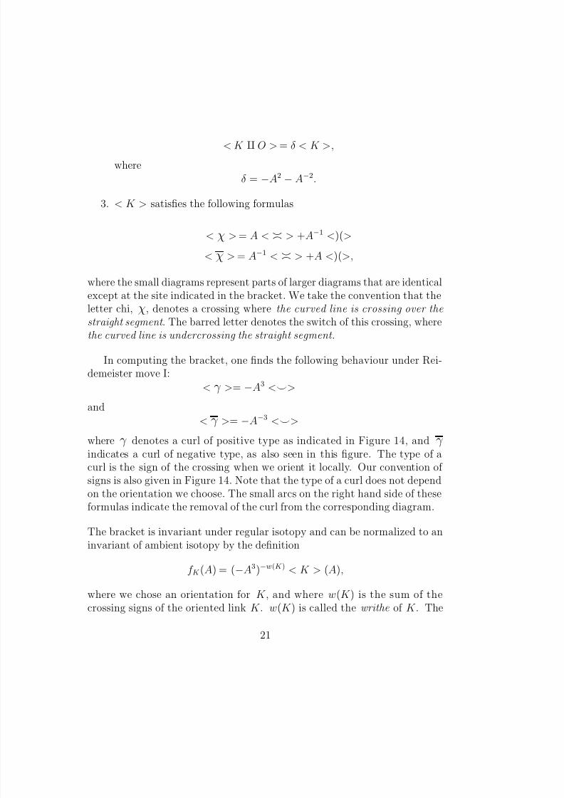
3. < K > satises the following formulas

< χ > = A < > + A− 1 < )(>

< χ > = A− 1 < > + A < )(>,

where the small diagrams represent parts of larger diagrams that are identicalexcept at the site indicated in the bracket. We take the convention that theletter chi, χ , denotes a crossing where the curved line is crossing over thestraight segment . The barred letter denotes the switch of this crossing, wherethe curved line is undercrossing the straight segment .

In computing the bracket, one nds the following behaviour under Rei-demeister move I:

< γ > = −A3 < >

and< γ > = −A− 3 < >

where γ denotes a curl of positive type as indicated in Figure 14, and γ indicates a curl of negative type, as also seen in this gure. The type of acurl is the sign of the crossing when we orient it locally. Our convention of signs is also given in Figure 14. Note that the type of a curl does not dependon the orientation we choose. The small arcs on the right hand side of theseformulas indicate the removal of the curl from the corresponding diagram.

The bracket is invariant under regular isotopy and can be normalized to aninvariant of ambient isotopy by the denition

f K (A) = ( −A3)− w(K ) < K > (A),

where we chose an orientation for K , and where w(K ) is the sum of thecrossing signs of the oriented link K . w(K ) is called the writhe of K . The

21



convention for crossing signs is shown in Figure 14. The original Jones poly-nomial, V K (t) [8] is then given by the formula

V K (t) = f K (t− 1/ 4).

or

or

+ -

+ +

- -

Figure 14 - Crossing Signs and Curls

One useful consequence of these formulas is the following switching formula

Aχ −A− 1χ = ( A2 −A− 2) .

Note that in these conventions the A-smoothing of χ is , while the A-smoothing of χ is >< . Properly interpreted, the switching formula abovesays that you can switch a crossing and smooth it either way and obtain a

three diagram relation. This is useful since some computations will simplifyquite quickly with the proper choices of switching and smoothing. Rememberthat it is necessary to keep track of the diagrams up to regular isotopy (theequivalence relation generated by the second and third Reidemeister moves).Here is an example. View Figure 15.

22



You see in Figure 15, a trefoil diagram K , an unknot diagram U and anotherunknot diagram U ′ . Applying the switching formula, we have

A− 1 < K > −A < U > = ( A− 2 −A2) < U ′ >

and < U > = −A3 and < U ′ > = ( −A− 3)2 = A− 6. Thus

A− 1 < K > −A(−A3) = ( A− 2 −A2)A− 6.

HenceA− 1 < K > = −A4 + A− 8 −A− 4.

Thus < K > = −A5 −A− 3 + A− 7.

This is the bracket polynomial of the trefoil diagram K.

Since the trefoil diagram K has writhe w(K ) = 3 , we have the normalizedpolynomial

f K (A) = ( −A3)− 3 < K > = −A− 9(−A5 −A− 3 + A− 7) = A− 4 + A− 12 −A− 16.

The asymmetry of this polynomial under the interchange of A and A− 1 provesthat the trefoil knot is not ambient isotopic to its mirror image.

K U U'

Figure 15 – Trefoil and Two Relatives

23



The bracket model for the Jones polynomial is quite useful both theoreti-cally and in terms of practical computations. One of the neatest applicationsis to simply compute, as we have done, f K (A) for the trefoil knot K and de-termine that f K (A) is not equal to f K (A− 1) = f − K (A). This shows that thetrefoil is not ambient isotopic to its mirror image, a fact that is much harderto prove by classical methods.

The State Summation. In order to obtain a closed formula for the bracket,we now describe it as a state summation. Let K be any unoriented linkdiagram. Dene a state , S , of K to be a choice of smoothing for each crossingof K. There are two choices for smoothing a given crossing, and thus there are2N states of a diagram with N crossings. In a state we label each smoothingwith A or A− 1 according to the left-right convention discussed in Property 3(see Figure 14). The label is called a vertex weight of the state. There aretwo evaluations related to a state. The rst one is the product of the vertexweights, denoted

< K |S > .The second evaluation is the number of loops in the state S , denoted

||S ||.Dene the state summation , < K > , by the formula

< K > =S

< K |S > δ || S ||− 1.

It follows from this denition that < K > satises the equations

< χ > = A < > + A− 1 < )(>,< K O > = δ < K >,

< O > = 1 .The rst equation expresses the fact that the entire set of states of a given

diagram is the union, with respect to a given crossing, of those states with anA-type smoothing and those with an A− 1-type smoothing at that crossing.The second and the third equation are clear from the formula dening thestate summation. Hence this state summation produces the bracket polyno-mial as we have described it at the beginning of the section.

24



8.2 Present Status of Links Not Detectable by theJones Polynomial

In this section we give a quick review of the status of our work [22] produc-ing innite families of distinct links all evaluating as unlinks by the Jonespolynomial.

A tangle (2-tangle) consists in an embedding of two arcs in a three-ball(and possibly some circles embedded in the interior of the three-ball) suchthat the endpoints of the arcs are on the boundary of the three-ball. Oneusually depicts the arcs as crossing the boundary transversely so that the

tangle is seen as the embedding in the three-ball augmented by four segmentsemanating from the ball, each from the intersection of the arcs with theboundary. These four segments are the exterior edges of the tangle, and areused for operations that form new tangles and new knots and links fromgiven tangles. Two tangles in a given three-ball are said to be topologically equivalent if there is an ambient isotopy from one to the other in the giventhree-ball, xing the intersections of the tangles with the boundary.

It is customary to illustrate tangles with a diagram that consists in a box(within which are the arcs of the tangle) and with the exterior edges ema-nating from the box in the NorthWest (NW), NorthEast (NE), SouthWest(SW) and SouthEast (SE) directions. Given tangles T and S , one denes thesum , denoted T + S by placing the diagram for S to the right of the diagramfor T and attaching the NE edge of T to the NW edge of S , and the SE edgeof T to the SW edge of S . The resulting tangle T + S has exterior edgescorresponding to the NW and SW edges of T and the NE and SE edges of S . There are two ways to create links associated to a tangle T. The numera-tor T N is obtained, by attaching the (top) NW and NE edges of T togetherand attaching the (bottom) SW and SE edges together. The denominatorT D is obtained, by attaching the (left side) NW and SW edges together andattaching the (right side) NE and SE edges together. We denote by [0] the

tangle with only unknotted arcs (no embedded circles) with one arc connect-ing, within the three-ball, the (top points) NW intersection point with theNE intersection point, and the other arc connecting the (bottom points) SWintersection point with the SE intersection point. A ninety degree turn of the tangle [0] produces the tangle [∞] with connections between NW and

26



SW and between NE and SE. One then can prove the basic formula for anytangle T

< T > = αT < [0]> + β T < [∞] >

where αT and β T are well-dened polynomial invariants (of regular isotopy)of the tangle T. From this formula one can deduce that

< T N > = αT d + β T

and

< T D > = αT + β T d.

We dene the bracket vector of T to be the ordered pair ( αT , β T ) anddenote it by br(T ), viewing it as a column vector so that br(T )t = ( αT , β T )where vt denotes the transpose of the vector v. With this notation the twoformulas above for the evaluation for numerator and denominator of a tanglebecome the single matrix equation

< T N >< T D > =

d 11 d br(T ).

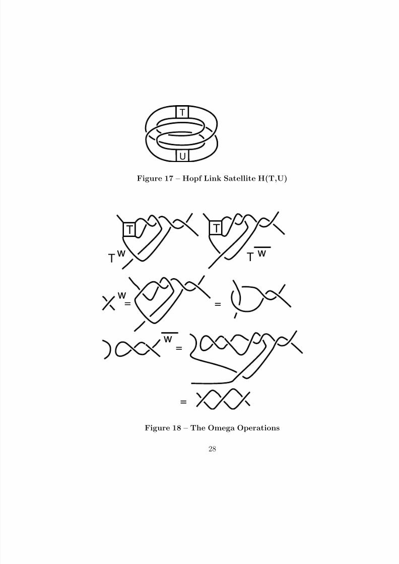
We then use this formalism to express the bracket polynomial for ourexamples. The class of examples that we considered are each denoted byH (T, U ) where T and U are each tangles and H (T, U ) is a satellite of theHopf link that conforms to the pattern shown in Figure 17, formed by claspingtogether the numerators of the tangles T and U. Our method is based on atransformation H (T, U ) −→H (T, U )ω, whereby the tangles T and U are cutout and reglued by certain specic homeomorphisms of the tangle boundaries.

This transformation can be specied by a modication described by a specicrational tangle and its mirror image. Like mutation, the transformation ωpreserves the bracket polynomial. However, it is more effective than mutationin generating examples, as a trivial link can be transformed to a prime link,and repeated application yields an innite sequence of inequivalent links.

27



T

U

Figure 17 – Hopf Link Satellite H(T,U)

T Tw w

w= =

w=

=

T T

Figure 18 – The Omega Operations

28



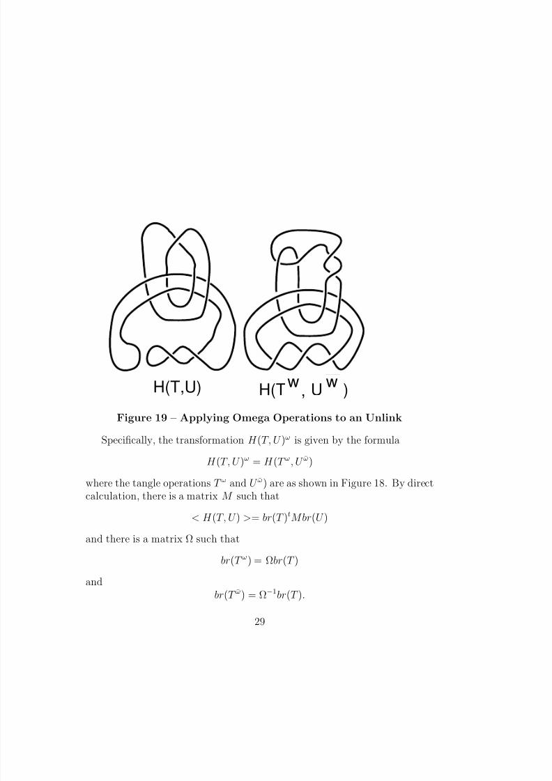
H(T,U) H(T w wU ),

Figure 19 – Applying Omega Operations to an Unlink

Specically, the transformation H (T, U )ω is given by the formula

H (T, U )ω = H (T ω, U ω)

where the tangle operations T ω and U ω) are as shown in Figure 18. By directcalculation, there is a matrix M such that

< H (T, U ) > = br(T )t Mbr(U )

and there is a matrix Ω such that

br(T ω) = Ωbr(T )

andbr(T ω) = Ω− 1br(T ).

29



One veries the identityΩt M Ω− 1 = M

from which it follows that < H (T, U ) > ω= < H (T, U ) > . This completesthe sketch of our method for obtaining links that whose linking cannot beseen by the Jones polynomial. Note that the link constructed as H (T ω, U ω)in Figure 19 has the same Jones polynomial as an unlink of two compo-nents. This shows how the rst example found by Thistlethwaite ts intoour construction.

9 From Quantum Topology to Khovanov Ho-mology

Quantum topology is the study of invariants of topological objects whoseproperties emulate partition functions in statistical mechanics, quantum me-chanics and quantum eld theory. The FKT model of the Alexander-Conwaypolynomial and the bracket model of the Jones polynomial were the rst ex-amples of such relationships with partition functions. The Jones polynomialwas generalized to a number of other polynomial invariants of links (theHomypt and Kauffman polynomials) and to so-called quantum invariantsof colored links and trivalent framed knotted graphs (the colorings corre-sponding to the irreducible representations of the SU (2)q quantum group).These colored invariants were used to create the Reshetikhin-Turaev invari-ants [26, 25] of closed oriented 3-manifolds. Simultaneously, invariants of three manifolds were discovered by Witten [27] in a quantum-eld theoreticapproach to invariants, using functional integrals. It was made clear at theheuristic level that the functional integral approach and the Reshetikhin-Turaev approach were equivalent, but radically different approaches to thesame structure. The combination of the two approaches led to the notionof topological quantum eld theories (TQFT’s) [2]. A TQFT is a functor

from a categories of closed surfaces (or higher dimensional manifolds) andtheir cobordisms, with appropriate additional structures, to the category of nite-dimensional vector spaces. This point of view can be used effectively tocapture the properties of the quantum group based invariants and to modelthe mathematical essence of the functional integral approach.

30



A new approach to invariants emerged in 1999 when Mikhail Khovanov[17] constructed a homology theory H(D) dened through diagrams D rep-resenting an oriented link L in three-space, so that the polynomial Eulercharacteristic χ (H(L)) of this theory is a version of the Jones polynomialof L, and the homology itself carries more topological information than theJones polynomial. Khovanov’s construction is an example of categorication.

The Khovanov theory introduces a new concept in quantum topology,namely that it is possible to transmute state summations to summations of modules and then to create topological invariants by taking an appropriatehomology or cohomology of these modules. These concepts bring the meth-ods of algebraic topology into the subject of quantum topology in a freshway. They suggest that the direct attempt to produce topological partitionfunctions for four-dimensional topology may have to undergo a signicant de-tour involving cohomological methods before it achieves success. Khovanovhomology and its generalizations have proved to be a powerful and usefultool for low dimensional topology.

We end this introduction to Formal Knot Theory with a sketch of the

Khovanov homology, as it is directly related to the bracket polynomial model.The reader will see that this is indeed a natural outgrowth of the bracketmodel.

Consider the two smoothings of a crossing. It is natural to put then to-gether as the top and the bottom of a bit of smooth saddle surface as shownin Figure 20. Then there is a topological evolution from one smoothing tothe other going through the critical level in the saddle where two lines crossone another. The saddle appears as a geometrical/topological transforma-

tion from one smoothing to the other. The question is, how could such atransformation be imaged in an algebraic or combinatorial structure to makedeeper versions of the bracket polynomial invariant? Khovanov’s beautifulidea is to regard the transformation from one smoothing to the other as aningredient for forming the differential for a chain complex.

31



A A-1d

A A-1

A-1A

∆

m

Figure 20 – Saddle Points and DifferentialsSpecically, one associates an algebra Ato each loop in a bracket poly-

nomial state S for the knot or link K. Then one takes the tensor product

A||S|| where ||S || is the number of loops in the state S. The n-th level of

32



the chain complex C (K ) is denoted C n (K ) and is dened to the the directsum of the modules A||S|| where S is a state with n sites of type A. Thedifferential in this complex is designed to take C n +1 (K ) to C n (K ). The differ-ential is built from the two possibilities for resmoothing a site, as illustratedin Figure 20. In one case two curves become a single curve. In the othercase a single curve is transformed into two curves. We have denoted thesetwo possibilities by m and ∆ respectively. Since each curve is associated toa copy of the algebra A, it follows that there should be maps of algebrasm : A A−→Aand ∆ : A−→A A. Thus the algebra needs a product mand a coproduct ∆. The differential always goes from a smoothing of type Ato a smoothing of type A− 1 when restricted to a given loop, or pair of loops

in a state. Since a resmoothing of a type A state changes it to a type A− 1

state, the number of type A states is reduced by one when the differential isperformed. The total differential from C n +1 (K ) to C n (K ) is assembled froma signed summation over all single-site maps as described above. The signsrequire ordering choices and we refer the reader to [3] for more information(where the complex is expressed in cohomology rather than homology).

A key point about this construction is illustrated in Figure 21. In orderthat the differential in the complex be well-dened and have the propertythat d2 = 0 , one needs that different orders of application of it will coincide.It is easiest to see this necessary compatibility condition by thinking of the

elementary bit of differential as m or ∆, depicted as a bit of saddle surfacebeginning with two loops and ending with one loop, or beginning with oneloop and ending with two loops. Then the compatibility corresponds to theequality of the compositions F = G = H indicated in Figure 21 as

F = ∆ m,

G = ( m 1) (1 ∆) ,

H = (1 ∆) (m 1).

These are the conditions for Ato be a Frobenius algebra [3]. For an exampleof an algebra satisfying these requirements, take

Ato have basis

1, X

with

1 acting as a multiplicative identity and

X 2 = m(X X ) = 0 ,

∆(1) = 1 X + X 1,

33



and∆( X ) = X X.

This algebra satises the requirements and produces an homology theorythat is invariant under the Reidemeister moves (when one takes into accountgrading changes that the moves can produce).

∆ m

F G H

Figure 21 – The Frobenius Algebra Conditions

Khovanov homology grows naturally out of the bracket state sum,creatinga new technique for obtaining topological information from the states of thelink diagram.

34



9.1 Knot Floer HomologyFinally, we mention the work of Ozsv ath and Szab o [23] on Heegard Floerhomology. This is a homology theory associated to knots that categories theAlexander Polynomial. The chain complex for this theory has a basis thatis in one-to-one correspondence with the states in the Formal Knot Theorymodel for the Alexander-Conway polynomial. At this writing, there is nostrictly combinatorial description for the differentials in the chain complexfor this homology theory. The theory appears to depend upon more complexgeometry than the Khovanov invariant.

References[1] J. W. Alexander, Topological invariants of knots and links, Trans. Amer.

Math. Soc. , Vol. 30, Issue 2, (April 1928), 275-306.

[2] M.F. Atiyah, The Geometry and Physics of Knots , Cambridge Univer-sity Press, 1990.

[3] D. Bar-Natan, On Khovanov’s categorication of the Jones polynomial.Algebraic and Geometric Topology , Vol. 2 (2002), pp. 337-370.

[4] J. H. Conway, An enumeration of knots and links and some of theiralgebraic properties, in Computational Problems in Abstract Algebra ,Pergammon Press, N.Y.,1970, pp. 329-358.

[5] R. H. Fox, A quick trip through knot theory. In “Topology of 3-Manifolds”, ed. by M. K. Fort Jr., Prentice Hall (1962), 120-167.

[6] R. H. Crowell and R. H. Fox, “Introduction to Knot Theory”, BlaisdellPub. Co. (1963).

[7] P. M. Gilmer and R. A. Litherland, The duality conjecture in formalknot theory, Osaka J. Math. Vol. 23, (1986), 275-306.

[8] V.F.R. Jones, A polynomial invariant of links via von Neumann algebras,Bull. Amer. Math. Soc. , 1985, No. 129, pp. 103-112.

35



[9] L.H. Kauffman, The Conway polynomial, Topology , 20 (1980), pp. 101-108.

[10] L. H. Kauffman, Formal Knot Theory , Princeton University Press, Lec-ture Notes Series 30 (1983).

[11] L.H. Kauffman, On Knots , Annals Study No. 115, Princeton University Press (1987)

[12] L.H.Kauffman, State Models and the Jones Polynomial, Topology ,Vol.26, 1987,pp. 395-407.

[13] L.H.Kauffman, New invariants in the theory of knots, Amer. Math.Monthly , Vol.95,No.3,March 1988. pp 195-242.

[14] L. H. Kauffman, “Knots and Physics”, World Scientic, Singapore/NewJersey/London/Hong Kong, 1991, 1994, 2001.

[15] L. H. Kauffman and S. L. Lins, Temperley-Lieb Recoupling Theory and Invariants of 3- Manifolds , Annals of Mathematics Study 114, PrincetonUniv. Press,1994.

[16] L. H. Kauffman, math.GN/0410329, Knot diagrammatics. ”Handbookof Knot Theory“, edited by Menasco and Thistlethwaite, 233–318, El-sevier B. V., Amsterdam, 2005.

[17] Mikhail Khovanov, A categorication of the Jones polynomial, DukeMath. J. 101 (2000), no. 3, 359–426.

[18] D. Rolfsen, “Knots and Links”, Publish or Perish Press (1987).

[19] K. Reidemeister, Knotentheorie , Chelsea Pub. Co., New York, 1948,Copyright 1932, Julius Springer, Berlin.

[20] M.B. Thistlethwaite, A spanning tree expansion of the Jones polynomial,Topology 26 no. 3 (1987), 297–309.

[21] M. Thistlethwaite, Links with trivial Jones polynomial, JKTR, Vol. 10,No. 4 (2001), 641-643.

36



[22] S. Eliahou, L. Kauffman and M. Thistlethwaite, Innite families of linkswith trivial Jones polynomial, Topology , 42 , pp. 155–169.

[23] P. Ozsvath and Z. Szab o, Heegard Floer homology and alternatingknots, Geometry and Topology , Vol. 7 (2003), 225-254.

[24] J. Propp, Lattice structure for orientations of graphs, MIT (1993), (un-published).

[25] N.Y. Reshetikhin and V. Turaev, Invariants of Three-Manifolds via linkpolynomials and quantum groups, Invent. Math. ,Vol.103,1991, pp. 547-597.

[26] V.G.Turaev, The Yang-Baxter equations and invariants of links, LOMIpreprint E-3-87, Steklov Institute, Leningrad, USSR., InventionesMath. ,Vol. 92, Fasc.3, pp. 527-553.

[27] Edward Witten, Quantum eld Theory and the Jones Polynomial, Com-mun. Math. Phys. ,vol. 121, 1989, pp. 351-399.

37

Louis H. Kauffman- Remarks on Formal Knot Theory

Documents

Transcript of Louis H. Kauffman- Remarks on Formal Knot Theory