Loss Cost Modeling vs. Frequency and Severity … Cost Modeling vs. Frequency and Severity Modeling...
23
Loss Cost Modeling vs. Frequency and Severity Modeling Jun Yan Deloitte Consulting LLP 2013 CAS Ratemaking and Product Management Seminar March 13, 2013 Huntington Beach, CA
Transcript of Loss Cost Modeling vs. Frequency and Severity … Cost Modeling vs. Frequency and Severity Modeling...

Loss Cost Modelingvs.
Frequency and Severity Modeling
Jun YanDeloitte Consulting LLP
2013 CAS Ratemaking and Product Management SeminarMarch 13, 2013
Huntington Beach, CA

Antitrust Notice• The Casualty Actuarial Society is committed to adhering strictly to
the letter and spirit of the antitrust laws. Seminars conductedunder the auspices of the CAS are designed solely to provide aforum for the expression of various points of view on topicsdescribed in the programs or agendas for such meetings.
• Under no circumstances shall CAS seminars be used as a meansfor competing companies or firms to reach any understanding –expressed or implied – that restricts competition or in any wayimpairs the ability of members to exercise independent businessjudgment regarding matters affecting competition.
• It is the responsibility of all seminar participants to be aware ofantitrust regulations, to prevent any written or verbal discussionsthat appear to violate these laws, and to adhere in every respectto the CAS antitrust compliance policy.

Description of Frequency-Severity Modeling
• Claim Frequency = Claim Count / ExposureClaim Severity = Loss / Claim Count
• It is a common actuarial assumption that:– Claim Frequency has an over-dispersed Poisson
distribution– Claim Severity has a Gamma distribution
• Loss Cost = Claim Frequency x Claim Severity• Can be much more complex

Description of Frequency-Severity Modeling
• A more sophisticated Frequency/Severity modeldesigno Frequency – Over-dispersed Poissono Capped Severity – Gammao Propensity of excess claim – Binomialo Excess Severity – Gammao Expected Loss Cost = Frequency x Capped Severity
+ Propensity of excess claim x Excess Severityo Fit a model to expected loss cost to produce loss cost
indications by rating variable

Description of Loss Cost ModelingTweedie Distribution
• It is a common actuarial assumption that:– Claim count is Poisson distributed– Size-of-Loss is Gamma distributed
• Therefore the loss cost (LC) distribution is Gamma-Poisson Compound distribution, called Tweediedistribution– LC = X1 + X2 + … + XN– Xi ~ Gamma for i {1, 2,…, N}– N ~ Poisson

Description of Loss Cost ModelingTweedie Distribution (Cont.)
• Tweedie distribution is belong to exponentialfamilyo Var(LC) = p
is a scale parameter is the expected value of LC p є (1,2)p is a free parameter – must be supplied by the modelerAs p 1: LC approaches the Over-Dispersed PoissonAs p 2: LC approaches the Gamma

Data Description
• Structure – On a vehicle-policy term level
• Total 100,000 vehicle records
• Separated to Training and Testing Subsets:– Training Dataset: 70,000 vehicle records– Testing Dataset: 30,000 Vehicle Records
• Coverage: Comprehensive

Numerical Example 1GLM Setup – In Total Dataset
• Frequency Model– Target
= Frequency= Claim Count /Exposure
– Link = Log– Distribution = Poison– Weight = Exposure– Variable =
• Territory• Agegrp• Type• Vehicle_use• Vehage_group• Credit_Score• AFA
• Severity Model– Target
= Severity= Loss/Claim Count
– Link = Log– Distribution = Gamma– Weight = Claim Count– Variable =
• Territory• Agegrp• Type• Vehicle_use• Vehage_group• Credit_Score• AFA
• Loss Cost Model– Target
= loss Cost= Loss/Exposure
– Link = Log– Distribution = Tweedie– Weight = Exposure– P=1.30– Variable =
• Territory• Agegrp• Type• Vehicle_use• Vehage_group• Credit_Score• AFA

Numerical Example 1How to select “p” for the Tweedie model?
• Treat “p” as aparameter forestimation
• Test a sequence of “p”in the Tweedie model
• The Log-likelihoodshows a smooth inverse“U” shape
• Select the “p” thatcorresponding to the“maximum” log-likelihood
Value p Optimization
Log-likelihood Value p
-12192.25 1.20
-12106.55 1.25
-12103.24 1.30
-12189.34 1.35
-12375.87 1.40
-12679.50 1.45
-13125.05 1.50
-13749.81 1.55
-14611.13 1.60

Numerical Example 1GLM Output (Models Built in Total Data)
Frequency Model Severity Model Frq * SevLoss Cost Model
(p=1.3)
Estimate Rating Factor Estimate Rating Factor Rating Factor EstimateRatingFactor
Intercept -3.19 0.04 7.32 1510.35 62.37 4.10 60.43
Territory T1 0.04 1.04 -0.17 0.84 0.87 -0.13 0.88Territory T2 0.01 1.01 -0.11 0.90 0.91 -0.09 0.91Territory T3 0.00 1.00 0.00 1.00 1.00 0.00 1.00……….. …… …….. …….. …….. …….. …….. …….. ……..
agegrp Yng 0.19 1.21 0.06 1.06 1.28 0.25 1.29agegrp Old 0.04 1.04 0.11 1.11 1.16 0.15 1.17agegrp Mid 0.00 1.00 0.00 1.00 1.00 0.00 1.00
Type M -0.13 0.88 0.05 1.06 0.93 -0.07 0.93Type S 0.00 1.00 0.00 1.00 1.00 0.00 1.00
Vehicle_Use PL 0.05 1.05 -0.09 0.92 0.96 -0.04 0.96Vehicle_Use WK 0.00 1.00 0.00 1.00 1.00 0.00 1.00

Numerical Example 1Findings from the Model Comparison
• The LC modeling approach needs less modelingefforts, the FS modeling approach shows moreinsights.
What is the driver of the LC pattern, Frequency or Severity? Frequency and severity could have different patterns.

Numerical Example 1Findings from the Model Comparison – Cont.
• The loss cost relativities based on the FSapproach could be fairly close to the loss costrelativities based on the LC approach, when Same pre-GLM treatments are applied to incurred losses
and exposures for both modeling approacheso Loss Cappingo Exposure Adjustments
Same predictive variables are selected for all the threemodels (Frequency Model, Severity Model and Loss CostModelThe modeling data is credible enough to support the
severity model
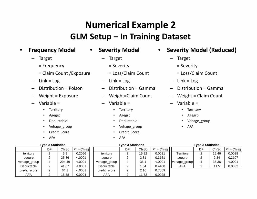
Numerical Example 2GLM Setup – In Training Dataset
• Frequency Model– Target
= Frequency= Claim Count /Exposure
– Link = Log– Distribution = Poison– Weight = Exposure– Variable =
• Territory• Agegrp• Deductable• Vehage_group• Credit_Score• AFA
• Severity Model– Target
= Severity= Loss/Claim Count
– Link = Log– Distribution = Gamma– Weight=Claim Count– Variable =
• Territory• Agegrp• Deductable• Vehage_group• Credit_Score• AFA
• Severity Model (Reduced)– Target
= Severity= Loss/Claim Count
– Link = Log– Distribution = Gamma– Weight = Claim Count– Variable =
• Territory• Agegrp• Vehage_group• AFA
Type 3 StatisticsDF ChiSq Pr > Chisq
territory 2 5.9 0.2066agegrp 2 25.36 <.0001
vehage_group 4 294.49 <.0001Deductable 2 41.07 <.0001credit_score 2 64.1 <.0001
AFA 2 15.58 0.0004
Type 3 StatisticsDF ChiSq Pr > Chisq
territory 2 15.92 0.0031agegrp 2 2.31 0.3151
vehage_group 4 36.1 <.0001Deductable 2 1.64 0.4408credit_score 2 2.16 0.7059
AFA 2 11.72 0.0028
Type 3 StatisticsDF ChiSq Pr > Chisq
Territory 2 15.46 0.0038agegrp 2 2.34 0.3107
vehage_group 4 35.36 <.0001AFA 2 11.5 0.0032

Numerical Example 2GLM Output (Models Built in Training Data)
Frequency Model Severity Model Frq * SevLoss Cost Model
(p=1.3)
EstimateRatingFactor Estimate
RatingFactor
RatingFactor Estimate
RatingFactor
Territory T1 0.03 1.03 -0.17 0.84 0.87 -0.15 0.86Territory T2 0.02 1.02 -0.11 0.90 0.92 -0.09 0.91Territory T3 0.00 1.00 0.00 1.00 1.00 0.00 1.00
…………… … …….
Deductable 100 0.33 1.38 1.38 0.36 1.43Deductable 250 0.25 1.28 1.28 0.24 1.27Deductable 500 0.00 1.00 1.00 0.00 1.00
CREDIT_SCORE 1 0.82 2.28 2.28 0.75 2.12CREDIT_SCORE 2 0.52 1.68 1.68 0.56 1.75CREDIT_SCORE 3 0.00 1.00 1.00 0.00 1.00
AFA 0 -0.25 0.78 -0.19 0.83 0.65 -0.42 0.66AFA 1 -0.03 0.97 -0.19 0.83 0.80 -0.21 0.81AFA 2+ 0.00 1.00 0.00 1.00 1.00 0.00 1.00

Numerical Example 2Model Comparison In Testing Dataset
• In the testing dataset, generate two sets of loss costScores corresponding to the two sets of loss costestimates– Score_fs (based on the FS modeling parameter estimates)– Score_lc (based on the LC modeling parameter estimates)
• Compare goodness of fit (GF) of the two sets of losscost scores in the testing dataset– Log-Likelihood

Numerical Example 2Model Comparison In Testing Dataset - Cont
GLM to Calculate GF Stat ofScore_fs
Data: Testing DatasetTarget: Loss CostPredictive Var: NonError: tweedieLink: logWeight: ExposureP: 1.15/1.20/1.25/1.30/1.35/1.40
Offset: log(Score_fs)
GLM to Calculate GF Stat ofScore_lc
Data: Testing DatasetTarget: Loss CostPredictive Var: NonError: tweedieLink: logWeight: Exposure
P: 1.15/1.20/1.25/1.30/1.35/1.40
Offset: log(Score_lc)

Numerical Example 2Model Comparison In Testing Dataset - Cont
GLM to Calculate GF StatUsing Score_fs as offset
Log likelihood from outputP=1.15 log-likelihood=-3749P=1.20 log-likelihood=-3699P=1.25 log-likelihood=-3673P=1.30 log-likelihood=-3672P=1.35 log-likelihood=-3698P=1.40 log-likelihood=-3755
GLM to Calculate GF StatUsing Score_lc as offset
Log likelihood from outputP=1.15 log-likelihood=-3744P=1.20 log-likelihood=-3694P=1.25 log-likelihood=-3668P=1.30 log-likelihood=-3667P=1.35 log-likelihood=-3692P=1.40 log-likelihood=-3748
The loss cost model has better goodness of fit.

Numerical Example 2Findings from the Model Comparison
• In many cases, the frequency model and the severitymodel will end up with different sets of variables.More than likely, less variables will be selected forthe severity modelData credibility for middle size or small size companies For certain low frequency coverage, such as BI…
• As a result F_S approach shows more insights, but needs additional
effort to roll up the frequency estimates and severityestimates to LC relativities In these cases, frequently, the LC model shows better
goodness of fit

A Frequently Applied MethodologyLoss Cost Refit
• Loss Cost RefitModel frequency and severity separatelyGenerate frequency score and severity score LC Score = (Frequency Score) x (Severity Score) Fit a LC model to the LC score to generate LC Relativities by
Rating VariablesOriginated from European modeling practice
• Considerations and SuggestionsDifferent regulatory environment for European market
and US marketAn essential assumption – The LC score is unbiased.Validation using a LC model

Constrained Rating Plan Study
• Update a rating plan with keeping certainrating tables or certain rating factorsunchanged
• One typical example is to create a rating tiervariable on top of an existing rating planCatch up with marketing competitions to avoid adverse
selectionManage disruptions

Constrained Rating Plan Study - Cont
• Apply GLM offset techniques• The offset factor is generated using the unchanged
rating factors.• Typically, for creating a rating tier on top of an
existing rating plan, the offset factor is given as therating factor of the existing rating plan.
• All the rating factors are on loss cost basis. It isnatural to apply the LC modeling approach forrating tier development.

How to Select Modeling Approach?• Data Related Considerations• Modeling Efficiency Vs. Business Insights• Quality of Modeling DeliverablesGoodness of Fit (on loss cost basis)Other model comparison scenarios
• Dynamics on Modeling ApplicationsClass Plan DevelopmentRating Tier or Score Card Development
• Post Modeling Considerations• Run a LC model to double check the parameter
estimates generated based on a F-S approach

An Exhibit from a Brazilian Modeler