Lori Dufour - FLM

THE USE OF BENTHIC INVERTEBRATE COMMUNITY STRUCTURE AND

CHEMICAL PARAMETERES IN THE ANALYSIS OF WATER QUALITY AT THREE

STREAMS WHERE A ROAD CROSSING IS PRESENT IN HALIBURTON FOREST

LORI DUFOUR

A FIELD RESEARCH REPORT SUBMITTED TO THE FACULTY OF APPLIED SCIENCE

AND ENGINEERING TECHNOLOGY IN PARTIAL FULFILLMENT OF THE

REQUIREMENTS FOR THE DIPLOMA OF ENVIRONMENTAL TECHNICIAN –

SAMPLING AND MONITORING

DIPLOMA PROGRAM IN ENVIRONMENTAL TECHNOLOGY

SENECA COLLEGE,

TORONTO, ONTARIO

MAY 2015

2

ABSTRACT Streams are an important aspect for watershed management as they are the initial

catchment for storm water runoff. It is important to monitor streams in order to

gain an understanding of the degree that organic pollution may have on an aquatic

ecosystem. This study examined two streams in Haliburton Forest where road

crossings are present using the control/impact study design. Results showed that

there was no indication of possible impairment at both streams between the

reference and exposure units. Because of time constraints, sampling three streams

for the purposes of statistical analysis could not be completed. Additional research

should be done to gain a clearer understanding of the impacts of organic pollution in

rural developments.

3

Acknowledgements I would like to thank my crew members, Hayley Tompkins and Alex Kosyakov, for

their hardwork, commitment, guidance and contributions to this report. I would

like to thank Nadia Kelton for her encouragement and allowing this trip to be able to

happen as I could not have asked for a better place to do my final project, to Carmen

Schlamb for her guidance and support throughout the entire ESM program, and to

Gary Pritchard for his vast knowledge of aquatic ecology that he has passed on with

great efficiency. Lastly, I would like to thank my family and friends for their

patience for the past 16 months while I have been completing this program

4

Table of Contents ABSTRACT ................................................................................................................................................ 2 ACKNOWLEDGEMENTS ........................................................................................................................ 3 1.0 INTRODUCTION ............................................................................................................................... 6 2.0 METHODS ........................................................................................................................................... 8 STUDY SITES ............................................................................................................................................................... 8 STUDY DESIGN ............................................................................................................................................................ 9 BIC INDICES ............................................................................................................................................................. 10 Hilsenhoff Biological Index (HBI) ............................................................................................................... 10 %EPT ....................................................................................................................................................................... 10 Equitability (ED) ................................................................................................................................................. 11 Diversity (D) ......................................................................................................................................................... 11

3.0 RESULTS .......................................................................................................................................... 12 4.0 DISCUSSION .................................................................................................................................... 13 5.0 CONCLUSION .................................................................................................................................. 14 REFERENCES .......................................................................................................................................... 16 GLOSSARY .............................................................................................................................................. 18 APPENDIX I – DATA FIELD SHEETS ................................................................................................ 19 APPENDIX II – RAW DATA ................................................................................................................ 28

5

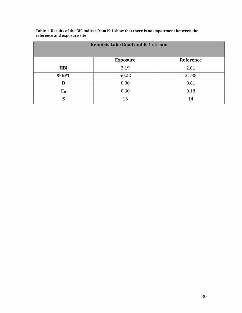
List of Tables Table 1 Results of the BIC indices from K-‐1 show that there is no impairment between the reference

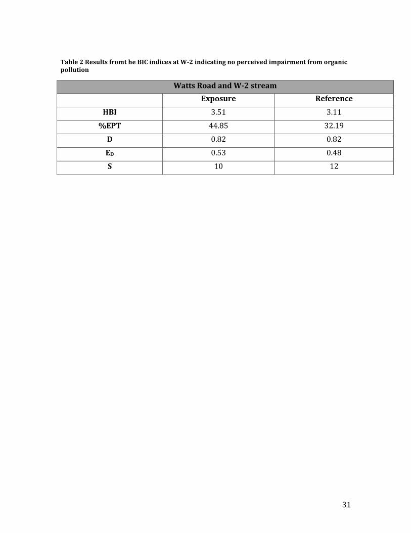
and exposure site ............................................................................................................................................................ 30 Table 2 Results fromt he BIC indices at W-‐2 indicating no perceived impairment from organic

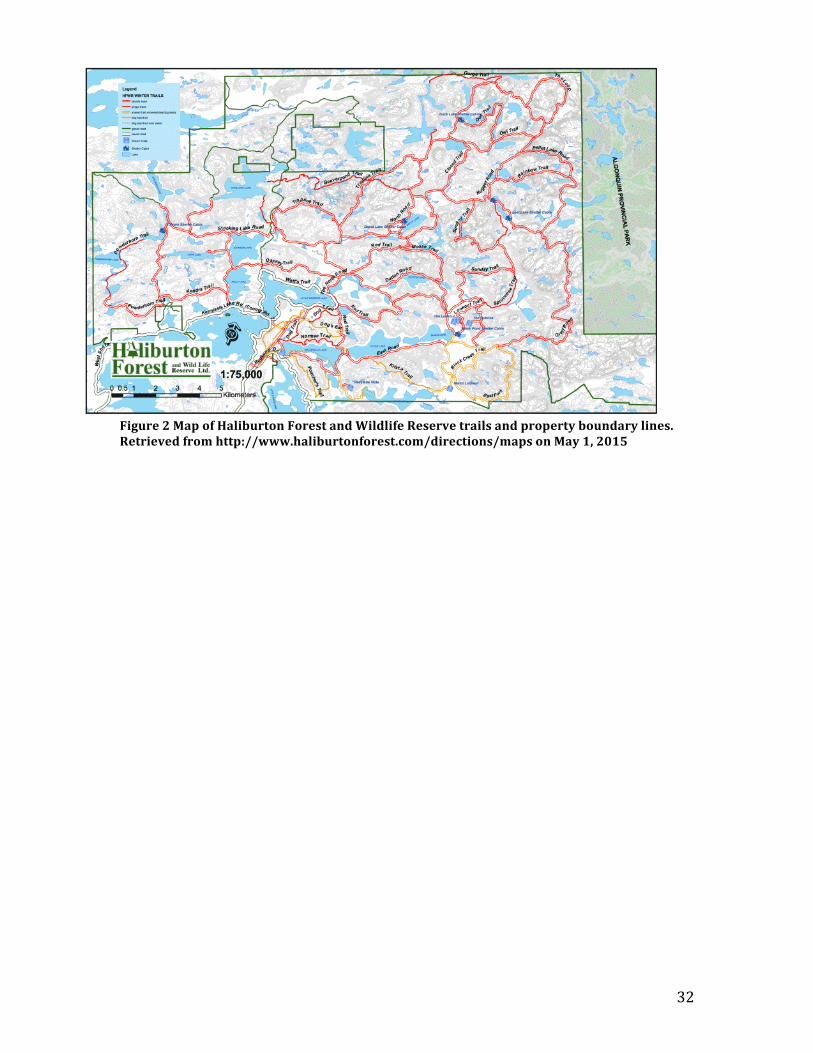
pollution .............................................................................................................................................................................. 31 List of Figures Figure 1 Map of Haliburton Forest and Wildlife Reserve trails and property boundary lines. Retrieved from http://www.haliburtonforest.com/directions/maps on May 1, 2015…………...32

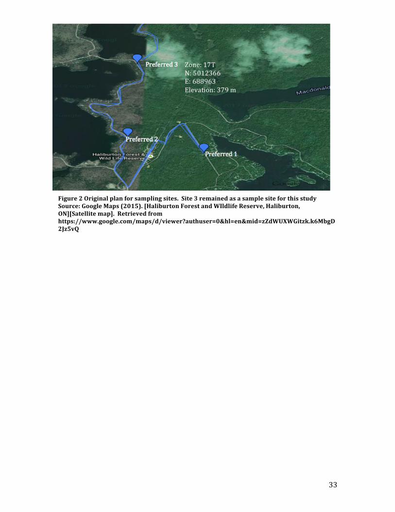
Figure 2 Original plan for sampling sites. Site 3 remained as a sample site for this study Source: Google Maps (2015). [Haliburton Forest and WIldlife Reserve, Haliburton, ON][Satellite map]. Retrieved from https://www.google.com/maps/d/viewer?authuser=0&hl=en&mid=zZdWUXWGitzk.k6MbgD2Jz5vQ …………………………………………………………………………………………………………………………………………………...33 Figure 3 Map location showing both sampling sites. One original site was used as site K-‐1 and backup 2 was used as site W-‐2 Source: Google Maps (2015). [ Haliburton Forest & WIldlife Reserve, Haliburton, ON] [satellite map]. Retrieved from https://www.google.com/maps/d/viewer?authuser=0&hl=en&mid=zZdWUXW…………………………..34 Figure 4 Upstream site photo of the exposure site at K-‐1. Author: Alex Kosyakov…………………………..35 Figure 5 Upstream site photo of the reference unit at site K-‐1. Author: Alex Kosyakov…………36

Figure 6 Upstream photo of the exposure unit at site W-‐2. Author: Alex Kosyakov………………………...37 Figure 7 Upstream photo of reference unit at site W-‐2. Author: Alex Kosyakov……………………………...38

6

1.0 INTRODUCTION

Watersheds are home to countless plants and animals that rely on the health

of these waters to survive. Watersheds are an important area of environmental

research because storm water runoff drains to other bodies of water, ultimately

carrying harmful substances that can alter the life histories of many aquatic species

(Panas, J., 2014). Considering these downstream impacts is important from a water

quality and restoration point of view. Streams are the initial catchment from

precipitation runoff and are ecologically important because of the goods and

services they provide to the environment (Kafle, et al., 2013). These services

include a source of clean drinking water, flood and erosion protection, groundwater

recharge, pollution reduction, and wildlife habitat.

Streams flow through industrialized area, cities, and towns where there are a

lot of road crossings. This gives the opportunity for pollution from automobiles and

agricultural practices to enter aquatic ecosystems (Delucchi, M.A, 2000). The most

common type of pollutants are oil, petroleum products, heavy metals, and nutrients

such as phosphorus (Vinodhini, R., & Narayanan, M., 2008). Heavy metals are

particularly concerning due to their toxicity, pervasiveness, and persistence. Metals

present in water are absorbed by fish and other aquatic organisms and tend to

bioconcentrate in the tissues of these organisms (Hsu, Selvaraj, & Agoramoorthy,

2006). This leads to metal toxicity and causes adverse biological effects on an

organism’s survival, activity, growth, metabolism, and reproduction (Blasius, B.J.,

2002). This diminishes the quality of the ecosystem as fish, birds, and aquatic plant

populations start to decline and ecosystem services are no longer being provided.

7

Streams are therefore the focus of a lot of environmental monitoring

research. Stream monitoring efforts are focused mainly on the assessment of the

benthic invertebrate community (Bailey, et al., 1998). Aquatic benthic invertebrates

play a significant role in understanding the health of streams, as they are universal,

species rich, sedentary, long lived, and they integrate conditions temporally .

Because of these reasons, benthic invertebrates are assigned different values based

on their tolerance to pollution in the water (Goodnight, C.J., 1973). Tolerance values

can be applied to the family level or the species level and ranges from 0.00 – 10.00,

where 0 indicates excellent water quality and 10.00 indicates very poor water

quality (Mandaville, 2012).

Using tolerance values can give an indication that a community is impacted,

but it should not be used to make decisions regarding management and

remediation. Instead, the most effective way to use the information available from a

community is to establish biocriteria, usually through testing a reference site to an

exposure site (Bailey, 1998). This involves testing a site exposed to a stressor

against a reference site that is not exposed to a stressor. For the purposes of this

study, only the control/impact approach will be used. The control/impact approach

focuses on a single reference site upstream of the stressor discharge and a test site

downstream of the stressor discharge (Jones, 2007).

This research project aimed to investigate if stream condition in Haliburton

Forest would be compromised due to pollutants from storm water runoff where

road crossings are present. Since Haliburton Forest is a property that is not

available to agriculture and heavy industrialization, it was hypothesized that stream

8

quality would not be compromised. Chemical analysis was also used as

supplementary data to explain any discrepancies between the reference site and the

test site.

2.0 METHODS

Study Sites

Research was conducted at Haliburton Forest and Wildlife Reserve located in

the Kennisis watershed (Figure 1). The Kennisis watershed is located in Haliburton

County, Ontario. Data was originally to be collected from three stream reaches at

road crossings within the watershed (shown as ‘preferred’ in figure 2) that were

previously identified before fieldwork commenced. However, due to time

constraints only two streams were sampled and only one stream was on the original

sampling plan (shown as preferred 3 and backup 2 in figure 3). The second sampling

site was identified as a backup site in the situation that any of the original sites were

not suitable for this study. For this reason, statistics applied to measures of central

tendency and one-‐way ANOVA was not completed.

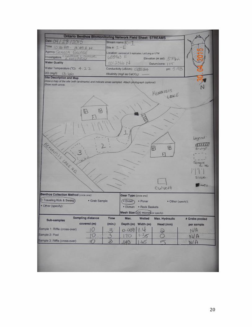
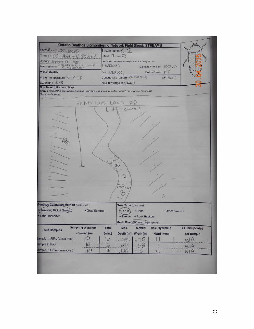
Site reconnaissance was conducted on Monday April 27, 2015. Site 1 (figure

4 and 5) was located on Kennisis Lake Road and was picked on April 28, 2015, and

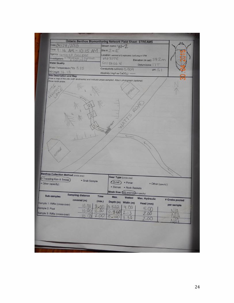
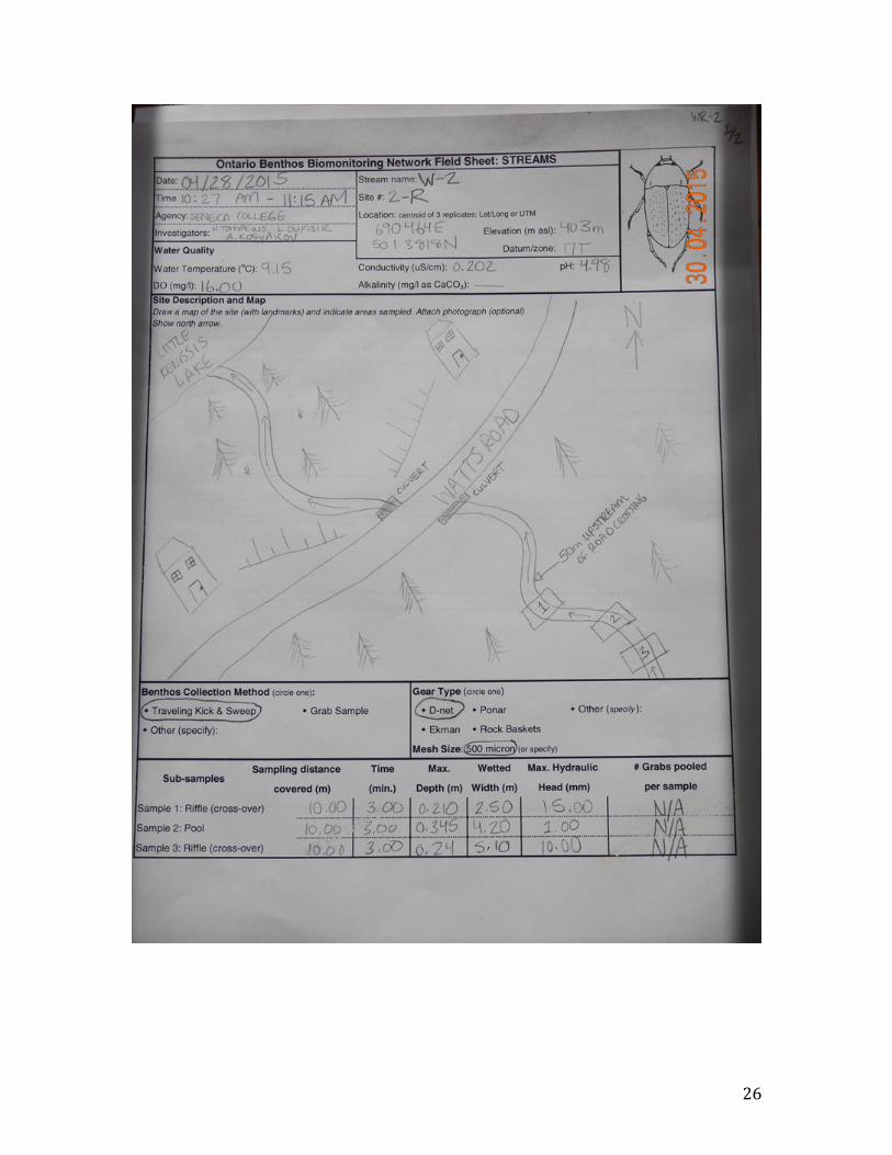
site 2 (figure) was located on Watts Road and was picked on April 29, 2015 (figure 6

and 7). Both of the stream names were unknown, so they were named based on the

road name. Therefore, the stream crossing at Kennisis Lake Road was named K-‐1

and the stream crossing at Watts Road was named W-‐2.

9

Study Design

Sample units for the reference and exposure sites was a stream reach and

was considered as the basic unit in which data was collected and followed the

control/impact study design specified in the Ontario Benthic Biomonitoring

Network (OBBN) protocol. Sample units were positioned in a longitudinal

configuration where the reference site was located 50 m upstream of a road

crossing and an exposure site immediately below the culvert outlet.

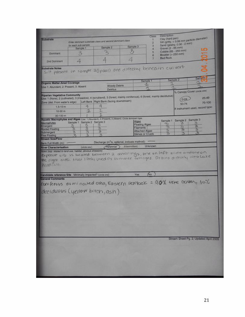
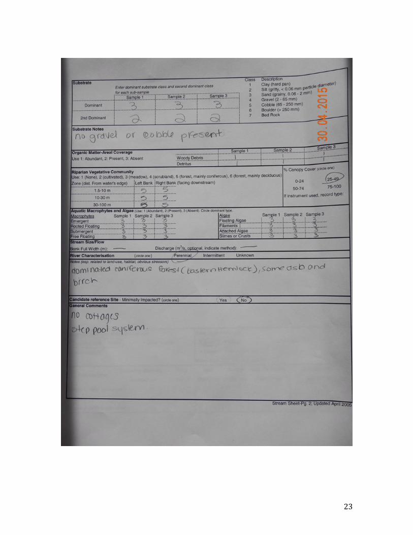
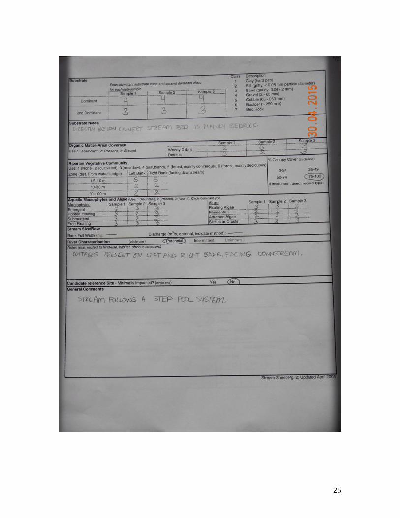
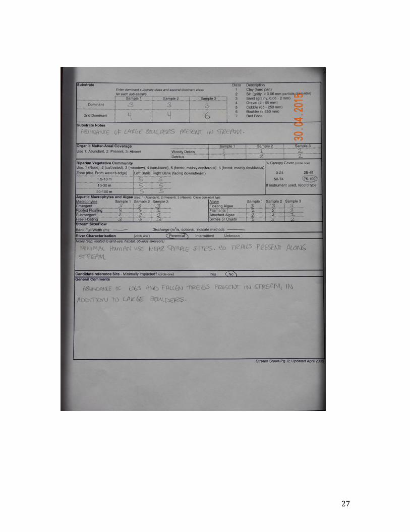
Data collected at each sample unit included water quality data, benthic

macroinvertebate community data, and physical habitat data, which included

substrate type, organic matter-‐areal coverage, riparian vegetative community,

aquatic macrophytes and algae, and tree cover.

Both the reference and exposure sampling unit consisted of three

subsamples, which consisted of a riffle, pool, riffle sequence. Each subsample was

measured for maximum depth (m), wetted width (m), and maximum hydraulic head

(mm). Maximum depth and wetted width were measured using a meter stick and

maximum depth was measured using a 30 m measuring tape. Water quality was

taken using a YSI 556 in the middle of the sample unit at both the reference and

exposure site. The YSI 556 was totally submerged into the water, but did not touch

the bottom of the streambed. The data taken from the YSI 556 were temperature

(oC), DO (mg/L), conductivity (µS/cm), and pH. Benthic macroinvertebrate

community was collected following the OBBN protocol. Invertebrates were collected

at each subsample by the travelling kick and sweep method using a 500-‐micron d-‐

net frame. Each subsample was kicked for 3 minutes and covered 10 m of sampling

10

area to meet the minimum 100-‐bug requirement at each subsample and 300 for

each sampling unit. Benthos were picked in the lab using the bucket sub-‐sampling

method (David et al., 1998) and were identified to the 27 family level as per the

OBBN standard.

BIC Indices

Hilsenhoff Biological Index (HBI) HBI, otherwise known as family biotic index (FBI), was used to calculate the water

quality of each stream sampling unit based on the benthos that were collected.

Tolerance values range from 0 – 10 where 0 would indicate excellent water quality

and 10 would indicate very poor water quality. The HBI is a single value for a

sampling unit and is based on the individual tolerance values for a taxon. HBI was

calculated using the following formula specified by Mandaville (2002):

𝐻𝐵𝐼 = Σ𝑥𝑖𝑡𝑖𝑛

xi = # of individuals within a taxon ti = tolerance value of a taxon

n = total number of organisms in the sample

%EPT Individuals belonging to the Ephemeroptera, Plecoptera, and Trichoptera families

are considered to be sensitive to pollution (Mandaville, 2002). Therefore, %EPT

was used because it considers the percentage of Ephemeroptera, Plecoptera and

Trichoptera in relation to the total number of animals in the sample and was

calculated as follows:

11

%𝐸𝑃𝑇 =Σ 𝐸,𝑃,𝑇

total individuals

Equitability (ED)

The Species Evenness Index (SEI), or equitability, is a measure of relative

abundance of the different taxa contributing to the richness in an area. The Species

Evenness Index quantifies how equal the community is. Species Evenness Index

values range from 0 to 1. Values closer to 0 indicate a community that is dominated

by only a few taxa, whereas values closer to 1 indicate that the community is more

evenly distributed. ED was calculated using the following formula adapted from

Beals, Gross, and Harrel (1999):

𝐸𝐷 =𝐷𝑠

D = Simpson’s diversity index s = total number of species in the community

𝐷 = 1/𝑝𝑖^2

pi = proportion of S made up of the ith species

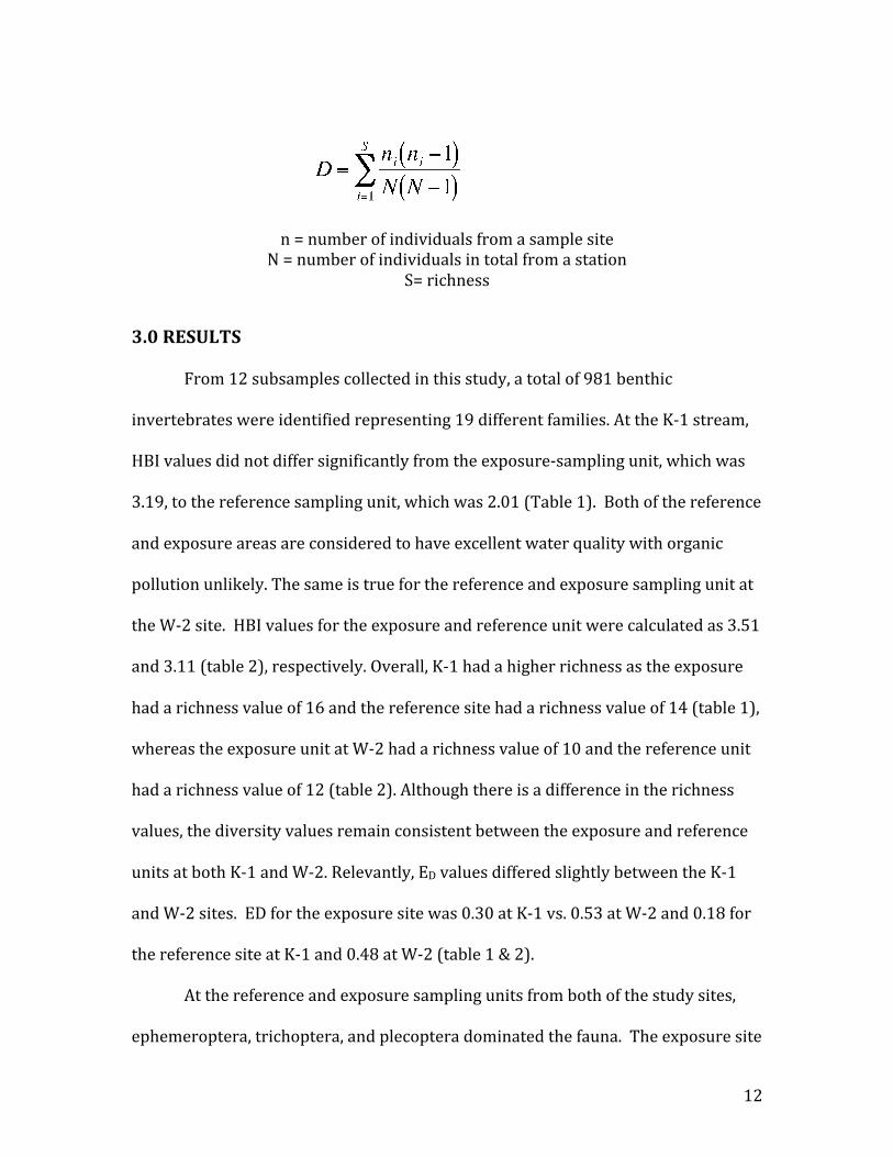
Diversity (D)

The Simpson’s Diversity Index (D, or SDI) measures diversity within the

benthic invertebrate community and provides information about rarity and

commonness of species in a community. This index places a greater weight on

common species from the population rather than the rare species. Values range

from 0 to 1. Values of 0, or close to 0, indicate a low level of diversity, while values

ranging closer to or equal to 1 indicate a high level of diversity. The Simpson’s

Diversity Index was calculated using the following formula:

12

n = number of individuals from a sample site N = number of individuals in total from a station

S= richness

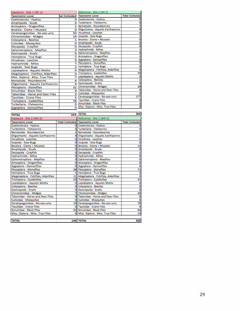
3.0 RESULTS From 12 subsamples collected in this study, a total of 981 benthic

invertebrates were identified representing 19 different families. At the K-‐1 stream,

HBI values did not differ significantly from the exposure-‐sampling unit, which was

3.19, to the reference sampling unit, which was 2.01 (Table 1). Both of the reference

and exposure areas are considered to have excellent water quality with organic

pollution unlikely. The same is true for the reference and exposure sampling unit at

the W-‐2 site. HBI values for the exposure and reference unit were calculated as 3.51

and 3.11 (table 2), respectively. Overall, K-‐1 had a higher richness as the exposure

had a richness value of 16 and the reference site had a richness value of 14 (table 1),

whereas the exposure unit at W-‐2 had a richness value of 10 and the reference unit

had a richness value of 12 (table 2). Although there is a difference in the richness

values, the diversity values remain consistent between the exposure and reference

units at both K-‐1 and W-‐2. Relevantly, ED values differed slightly between the K-‐1

and W-‐2 sites. ED for the exposure site was 0.30 at K-‐1 vs. 0.53 at W-‐2 and 0.18 for

the reference site at K-‐1 and 0.48 at W-‐2 (table 1 & 2).

At the reference and exposure sampling units from both of the study sites,

ephemeroptera, trichoptera, and plecoptera dominated the fauna. The exposure site

13

at K-‐1 had a %EPT of 50.22, but the reference site shows a %EPT value at 21.85

(table).

4.0 DISCUSSION Overall, these findings may suggest that organic pollution from road

crossings in a rural, remote location does not likely present a great risk to stream

quality. Likewise, benthic invertebrate community indices detected little or no

difference in the benthic assemblages between the exposure and reference units at

each site.

However, there is a discrepancy regarding the %EPT values at the K-‐1 site.

At the K-‐1 site the dominant substrate at the exposure site was classified as sand

and gravel, but had higher levels of silt as compared to the reference site. According

to Angradi (1999), and Hogg and Norris (1991), %EPT values decrease with

increased sedimentation. Additionally, only 223 organisms were counted at the

exposure site compared to 302 at the reference site. The higher %EPT value can be

attributed to the smaller ratio of EPT to total organisms. This suggests that

additional sampling needs to be conducted to make more accurate conclusions for

this discrepancy.

The exposure unit at the W-‐2 site yielded significantly less organisms than

the reference unit at the same site. This can possibly be explained by the high flow of

the water and the substrate type. The exposure site at W-‐2 was dominated by gravel

and coarse sand sediments and had very high flow as it exited the culvert.

Additionally, directly below the culvert, the substrate was bedrock. The high

14

velocity of the water may have caused the benthos to be dislodged and the coarse

sediments may not have provided optimal habitat for benthic invertebrates (Quinn

& Hickey, 1994; Jowett et al., 1991; Quinn, J.M., et. al, 1997).

HBI values for the exposure and reference sites at both K-‐1 and W-‐2 are low

and provide indication that the water quality is excellent and organic pollution is

unlikely (Mandaville, 2002). This is consistent with the finding that with increased

concentrations of organic pollution, DO decreases (Lenntech Inc., 2015).

The miniscule difference in the indices indicates that further sampling needs

to be completed in order to make an accurate conclusion regarding the stream

health at Haliburton Forest. The original plan to sample three streams was not

viable. Therefore, statistical analysis was not permissible for comparison purposes.

As a result, it is recommended that site reconnaissance be completed before any

type of fieldwork is completed. Additionally, the HBI values that were calculated for

the exposure and reference units did not consider organisms from the

ceratopogonidae family group or the miscellaneous diptera group as their tolerance

values were not indicated. In order to gain more accurate information for HBI

values, more time can be spent identifying organisms to the species level. However,

the correct laboratory equipment, and time is required to obtain a correct

identification.

5.0 CONCLUSION

From these results, it is shown rural streams do not show any indication of

impact from organic pollution coming from road crossings. Additionally, it is

15

recommended that more research needs to be completed in order to make accurate

and confident conclusions regarding the water quality of streams in a rural area. It

is also important to ensure that site reconnaissance is completed thoroughly to

ensure that the proper amount of sampling sites is available to conduct statistical

analysis.

16

REFERENCES Angradi, T.R. (1999). Fine sediment and macroinvertebrate assemblagesin

Appalocian streams: a field experiment with biomonitoring applications. Journal of North American Benthological Society 18(1): 49-‐66.

Bailey, R., et al. (1998). Biological assessment of freshwater ecosystems using a

reference condition approach: comparing predicted and actual benthic invertebrate communities in Yukon streams. Freshwater Biology 39: 765-‐774.

Beals, M., Gross, L., and Harrell, S. (1999). Diversity Indices: Simpson’s D and E.

Retrived from http://www.tiem.utk.edu/~gross/bioed/bealsmodules/simpsonDI.html

Blasius, B.J., Merritt, R.W. (2002). Field and laboratory investigations on the effects

of road salt (NaCl) on stream macroinvertebrate communities. Environmental Pollution 120 219-‐231.

David. S.M., Somers, K.M., Reid, R.A., Hall, R.J., and Girard, R.E. (1998). Sampling

Protocols for the rapid bioassessment of streams and lakes using benthic macroinvertebrates: second edition. Ontario Ministry of Environment, Queens Printer for Ontario, Toronto.

Delucchi, M.A. (2000). Environmental externalities of motor-‐vehicle use in the U.S.

Journal of transport Economics and Policy 34, 135-‐168 Goodnight, C.J. (1973). The use of aquatic macroinvertebrates as indicators of

stream pollution. Transactions of the American Microscopical Society 92(1): 1-‐13.

Hogg, I.D. and R.H. Norris. (1991). Effects of runoff from land clearing and urban

development on the distribution and abundance of macroinvertebrates in pool area of a river. Aust. J. Mar. Freshwater Res. 42:50718

Hsu, M. J., Selvaraj, K., & Agoramoorthy, G. (2006). Taiwan's industrial heavy metal

pollution threatens terrestrial biota. Environmental Pollution, 143(2), 327-‐334.

Jones, C., et. al. (2007). Ontario Benthos Biomonitoring Network: Protocol Manual,

Ontario Ministry of the Environment. Retrieved on 1 May 2015 from http://www.saugeenconservation.com/download/benthos/2009/OBBN%20Protocol%20Manual.pdf

Jowett, I. G., et. al.(1991): Microhabitat preferences of benthic invertebrates and the development of generalised Deleatidium spp. habitat suitability curves,

17

applied to four New Zealand rivers. New Zealand journal of marine andfreshwater research 25: 187-‐200

Kafle, A., et. al. (2013). Assemblage structure of chironimidae (diptera: insect) from wadeable streams of the northern glaciated plains, south Dakota, USA. Proceedings of the South Dakota Academy of Science. Vol. 92.

Lenntech Inc. (2015). Organic Compounds in Freshwater. Retrieved from http://www.lenntech.com/aquatic/organic-‐pollution.htm

Mandaville, S.M. “Benthic Macroinvertebrates in Freshwater – Taxa Tolerance Values, Metrics, and Protocols” Soil & Water Conservation of Metro Halifax (2002). Web. 1 May 2015.

Panas, J., et. al. (2014). Bioassessment of benthic macroinvertebrates of the middle penns creek, Pennsylvania watershed. Journal of the Pennsylvania Academy of Science 88(1): 57-‐62.

Quinn, J.M., et. al. (1997). Land use effects on habitat, water quality, periphyton, and benthic invertebrates in Waikato, New Zealand, hill country streams, New Zealand Journal of Marine and Freshwater Research, 31(5), 579-‐597, DOI: 10.1080/00288330.1997.9516791

Quinn, J. M.; Hickey, C. W.; Linklater, W. (1996). Hydraulic influences on periphyton and benthic macroinvertebrates: simulating the effects of upstream bed roughness. Freshwater biology 35: 301-‐309.

Vinodhini, R., & Narayanan, M. (2008). Bioaccumulation of heavy metals in organs of fresh water fish Cyprinus carpio (Common carp). International Journal of Environmental Science & Technology, 5(2), 179-‐182.

18

GLOSSARY biomonitoring the process of sampling, evaluating and reporting on ecosystem condition using biological indicators (Jones, 2007)

pool a stream segment characterized by slow flow and a constant surface elevation; in alluvial systems, typically occur along the outside bend of a meander, where the thalweg is adjacent to the stream bank at bank-‐full discharge (Jones, 2007)

richness the number of taxa found (Jones, 2007)

riffle a stream segment having fast, sometimes turbulent flow and typically shallow depth; typically exibits an obvious local surface elevation change; in alluvial systems, typically occurs at a cross-‐over (Jones, 2007)

Sampling Unit sampling unit for streams; a segment of stream containing a minimum of 2 riffles and one pool; in alluvial streams, often defined as 1 meander wavelength, beginning and ending at a cross-‐over; where there is no discernable pool-‐riffle sequence, may be defined as 14-‐20 times the bank-‐full width (Jones, 2007)

sub-‐sample a benthos sample collected from either a pool or riffle transect in a stream Sampling Reach; a portion of a sample to be picked (Jones, 2007)

test site a site where biological condition or health is questioned (Jones, 2007)

19

APPENDIX I – Data Field Sheets

28

APPENDIX II – Raw Data

30

Table 1 Results of the BIC indices from K-‐1 show that there is no impairment between the reference and exposure site

Kennisis Lake Road and K-‐1 stream

Exposure Reference

HBI 3.19 2.01 %EPT 50.22 21.85 D 0.80 0.61

ED 0.30 0.18 S 16 14

31

Table 2 Results fromt he BIC indices at W-‐2 indicating no perceived impairment from organic pollution

Watts Road and W-‐2 stream Exposure Reference

HBI 3.51 3.11

%EPT 44.85 32.19

D 0.82 0.82 ED 0.53 0.48

S 10 12

32

Figure 2 Map of Haliburton Forest and Wildlife Reserve trails and property boundary lines. Retrieved from http://www.haliburtonforest.com/directions/maps on May 1, 2015

33

Figure 2 Original plan for sampling sites. Site 3 remained as a sample site for this study Source: Google Maps (2015). [Haliburton Forest and WIldlife Reserve, Haliburton, ON][Satellite map]. Retrieved from https://www.google.com/maps/d/viewer?authuser=0&hl=en&mid=zZdWUXWGitzk.k6MbgD2Jz5vQ

Zone: 17T N: 5012366 E: 688963 Elevation: 379 m

34

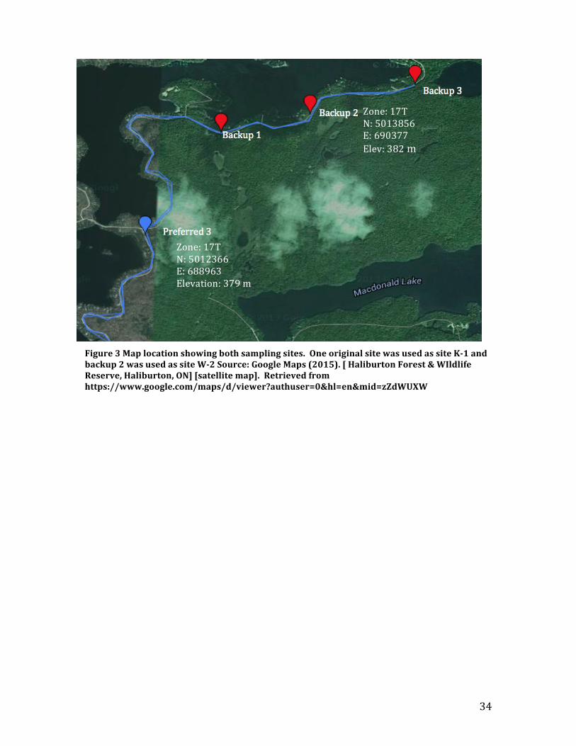
Figure 3 Map location showing both sampling sites. One original site was used as site K-‐1 and backup 2 was used as site W-‐2 Source: Google Maps (2015). [ Haliburton Forest & WIldlife Reserve, Haliburton, ON] [satellite map]. Retrieved from https://www.google.com/maps/d/viewer?authuser=0&hl=en&mid=zZdWUXW

Zone: 17T N: 5012366 E: 688963 Elevation: 379 m

Zone: 17T N: 5013856 E: 690377 Elev: 382 m

35

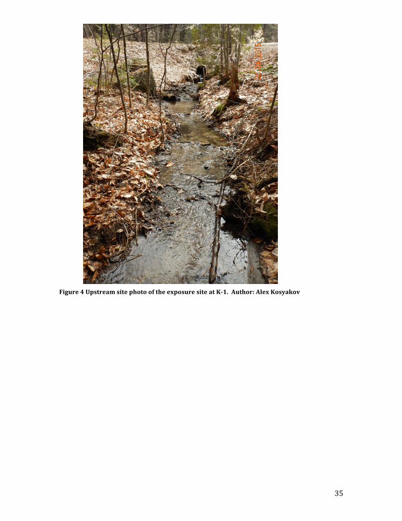
Figure 4 Upstream site photo of the exposure site at K-‐1. Author: Alex Kosyakov

36

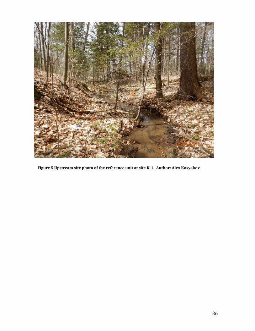
Figure 5 Upstream site photo of the reference unit at site K-‐1. Author: Alex Kosyakov

37

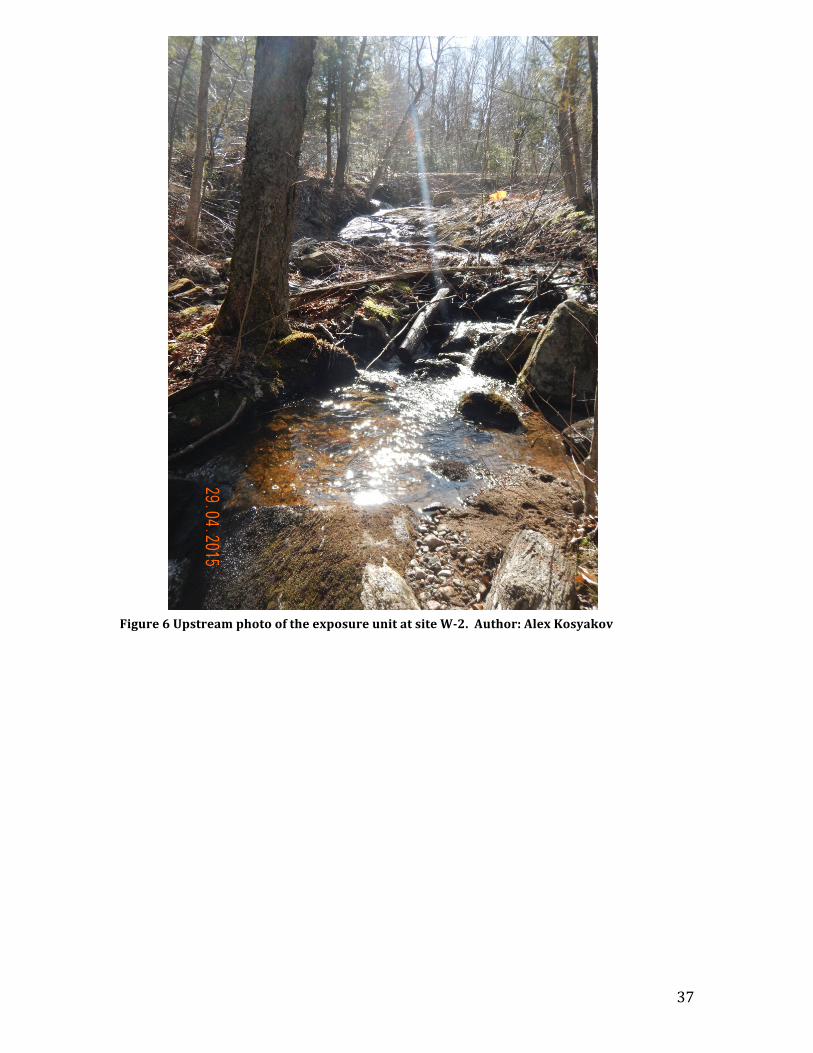
Figure 6 Upstream photo of the exposure unit at site W-‐2. Author: Alex Kosyakov

38

.

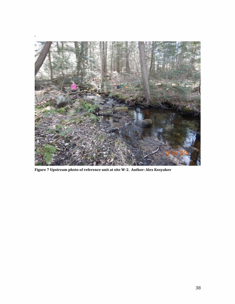
Figure 7 Upstream photo of reference unit at site W-‐2. Author: Alex Kosyakov

Lori Dufour - FLM

Documents

Transcript of Lori Dufour - FLM