Demographic Research a free, expedited, online journal of peer-reviewed research and commentary in the population sciences published by the Max Planck Institute for Demographic Research Doberaner Strasse 114 · D-18057 Rostock · GERMANY www.demographic-research.org

DEMOGRAPHIC RESEARCH VOLUME 1, ARTICLE 3 PUBLISHED 25 AUGUST 1999 www.demographic-research.org/Volumes/Vol1/3/ DOI: 10.4054/DemRes.1999.1.3

Longevity and month of birth Evidence from Austria and Denmark

Gabriele Doblhammer

© 1999 Max-Planck-Gesellschaft.

Longevity and month of birth:Evidence from Austria and Denmark.

Gabriele DoblhammerMax Planck Institute for Demographic Research

Rostock, Germany

AbstractThis article shows that in two European countries, Austria and Denmark, a person’s

life span correlates with his or her month of birth. It presents evidence that this pattern is notthe result of the seasonal distribution of death. It also shows that the seasonal pattern inlongevity cannot be explained by the so-called “birthday effect”– the alleged tendency ofpeople to die shortly after their birthday. The article concludes with a discussion of possiblesocial and biological mechanisms related to a person’s season of birth that might influence lifeexpectancy.

1 IntroductionOne of the first to describe differences in life span according to month of birth was

Ellsworth Huntington. In his book “Season of Birth” [10] he presents data on longevity bymonth of birth based on genealogical memoirs of families from different regions of the UnitedStates. For all regions he found that people born in February or March live decidedly longerthan those born in July or August.

A study of Japanese males born before 1890 [14] found that those born between Mayand July have a lower life expectancy after age 70 to 75 than those born in other months of thesame year. Recent research on babies born in rural Gambia indicates that those born during thedry season suffer higher mortality later in life than those born during the wet season [15].

Huntington’s findings stimulated a long line of research on season of birth and thelikelihood of mental disorders, e.g. schizophrenia (for a review of 250 studies, see [12, 16, 19,21]), Alzheimer’s disease [22], and autistic disorder [3]. Most of these studies foundsignificant differences in the risk of developing the respective disease according to season ofbirth. Findings on cancer patients have also revealed significant seasonality in life spanaccording to month of birth [17, 24].

Up to now studies about the relationship between month of birth and longevity haveused comparatively small data samples. For example, Huntington’s results are based ongenealogical information for about 39,000 persons. Some of the data samples were confined toselected groups: Miura’s findings are based on graduates of the Tokyo medical school and onasylum inmates, each group numbering about 400 people.

In this study I use data for total populations to investigate the question of whether ornot month of birth and life span are related. I employ two different data sources for twodifferent countries: Austria and Denmark. The Austrian data are based on vital statistics. Theexact date of birth and the exact date of death are known for each person who died between1988 and 1996. Only deaths after age 50 are considered. For the years 1990 to 1997 the causeof death is also reported. The Danish data consist of the total population aged 50+ on 1 April1968. These people were then followed until their death or until August 1998.

The result of this study suggests that life span and month of birth are in fact related.Having determined this, I then pay particular attention to the question of whether or not thisrelationship can be explained by factors that become active at the end of one’s life. I considertwo factors: first, the impact of the seasonal distribution of mortality on life span and, second,the “birthday-effect”. The latter refers to the alleged tendency of people to die shortly after

their birthday. I show in this study that neither factor can explain the relationship betweenmonth of birth and life span. Furthermore, I find cause to question recent results that found acorrelation between birthday and the time of death (e.g. [5, 23]).

The article closes with a discussion of possible mechanisms that may explain therelationship between month of birth and longevity.

2 Data & Method

2.1 DataMy analysis of the relationship between month of birth and life expectancy is based on twodifferent sets of data. For Austria the exact dates of birth and death are known for all 302,412men and 379,265 women who died between 1988 and 1996 at ages 50 and above. Causes ofdeath are given for 460,649 persons for the years 1990 to 1997.

The Danish data consist of a mortality follow-up of all Danes who were at least 50years old on 1 April 1968; 1,371,003 people were followed until their death or until the end ofthe observation period (week 32 of 1998). All these people were either born in Denmark(1,304,959 individuals) or their place of birth is unknown (66,044 individuals). The studyexcludes 1,994 people who were lost to the registry during the observation period. Amongthose who are included in the study, 85.5% (1,176,494 individuals) died before week 32 of1998; 14% (192,515 individuals) were still alive.

To test whether the seasonal distribution of births changes with age in Austria Icollected data on the number of births per month for the years 1880 to 1907. Only theGerman-speaking regions of the Austro-Hungarian Empire are included. The data are takenfrom the annual publications of the Central Bureau of Statistics (Statistisches Jahrbuch 1880 -1907).

2.2 MethodsFor Austria I estimated further life expectancy at age 50 by calculating the average of the exactages at death; for Denmark further life expectancy at age 50 was calculated on the basis of lifetables that were corrected for left truncation. This was achieved by calculating occurrence andexposure matrices which take into account an individual’s age on 1 April 1968. For example,a person who was 70 at the beginning of the study and who died at age 80 enters theexposures for ages 70 to 80 but is not included in the exposures for ages 50 to 69. Whencalculating the life tables, I estimated the central age-specific death rate 2 µ x based on theoccurrence-exposure matrix for two-year age-groups. The corresponding life table mortalityrate 2 q x is derived by the Greville Method [9].

For both countries, results are presented as the difference between the mean age atdeath of people born in a specific week and the average mean age at death in the study period.

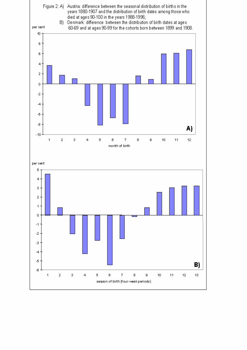
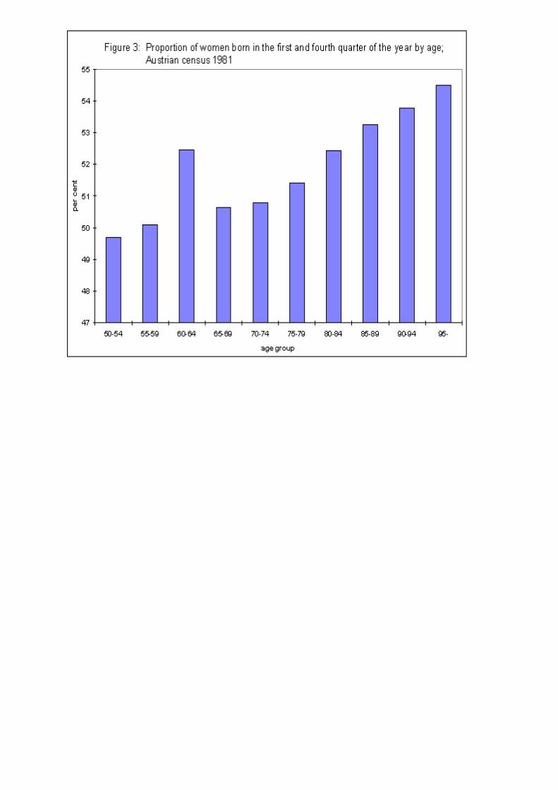
If people born in a specific month experience a higher mortality risk than others, thedistribution of birth dates of the total population changes with age [20]. To test this for AustriaI compared the monthly distribution of the number of births in the years 1880 to 1907 with thedistribution of birthdays among those who died at ages 90–99 in the years 1988 to1996. I alsocalculated for five-year age-groups the proportion of women in the 1981 census born inwinter. For Denmark I compared the distribution of birthdays of the survivors of the cohortsborn between 1899 and 1908 at ages 60–69 and 90–99.

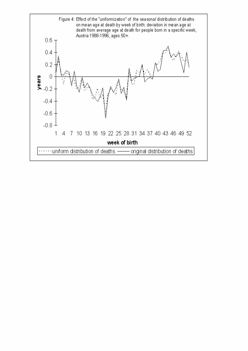
To test whether the seasonal distribution of deaths explains the differences in life span,the distribution of deaths was “uniformized” in the Austrian data set. The dates of death were

redistributed such that over the year they follow a uniform distribution, while their rank orderremains unchanged. In other words, the weeks of death d(t) are sorted thatd(1)<=...<=d(t)<=...<= d(n), with n equals the total number of deaths. Under a uniform

distribution in

=52

deaths will be observed in each week. Then the k-th death is reassigned to

week d(j), with jk

i=

−

+

11 , the integer part of the expression inside the brackets (e.g. if

the total number of deaths n equals 1040 then in each week i=20 persons should have died.Then the 65th person who has died is reassigned to week 4.) Average age at death accordingto week of birth is then recalculated based on d(j). This redistribution slightly increases the lifespan of people who died at the beginning of the year while it reduces the life span of thosewho died at the end of the year. If the seasonal pattern in life span is in fact caused by theseasonal distribution of deaths alone, the differences in life span should then disappear.

The longitudinal nature of the Danish data set allows me to model ( )µ x , the force ofmortality at age x, directly. The general mathematical specification of the model is

( ) ( ) ( )µ µ βx x y xi ii

=

∑0 exp{1}

where ( )µ x is a function of the baseline hazard ( )µ0 x ; the value of the covariate ( )y xi andthe regression coefficient βi that measures the effect of the covariate i on the force ofmortality.

In this model the baseline hazard ( )µ0 x is piecewise constant. The model assumes thatthe age-specific death rate for five-year age groups j follows a step function and that the deathrate within the five-year age groups is constant.Thus,

( )µ0 x a j= with j = 50-54, 55-59, 60-64, 65-69, 70-74, 75-79, 80-84, 85-89, 90+ {2}

All other covariates are sets of binary variables that represent the levels of categoricalcovariates. The following covariates are included:• month of birth [MOB]. This variable divides the year into thirteen periods, each consisting

of four weeks. Week one starts at day one, week two at day eight, and so forth;• time lived since the last birthday [TSLB]. This covariate divides the year into three

periods: (1) the twelve weeks immediately following an individual’s birthday (the week ofbirthday is defined as week one), (2) week 13 to week 40 (28 intermediary weeks) and (3)the twelve weeks before an individual’s next birthday (week 41 to week 52). This variableis defined for each year of an individual’s life starting with 1 April 1968;

• current month, which is measured in 13 four-week periods;• period: the years are divided into the six groups 1968-1974, 1975-1979, 1980-1984, 1985-

1989, 1990-1994, 1995-1998.• birth cohort: 1860-1879, 1880-1889, 1890-1899, 1900-1909, 1910-1918.

The first and the last covariate are independent of time. The other three covariates are time-varying. The second and the third variable account for two factors: first, for the possibility of a‘birthday-effect’ and second, for the seasonality in mortality. If they are both included at thesame time in one model, the model does not converge; probably this is due to the highcorrelation between the two variables [Note 1].

Period and cohort effects cannot be included simultaneously in a model that accountsfor age effects. Thus, four models were estimated. Model 1a includes sex, period, month ofbirth and current month; Model 1b uses the same covariates but adjusts for cohort factorsinstead of period factors. Model 2a includes sex, period and the second-order interaction term“time period since last birthday” x “month of birth”; Model 2b is similar to the latter modelbut adjusts for cohort factors. The two last models include a full set of second-orderinteraction terms between “month of birth” and “time period since last birthday” in order toaccount for the seasonal differences in the risk of mortality. The interaction is modelled by 38dummy variables, each representing a [MOB, TSLB] pair, with the (born in week 1-4, 1-12weeks since last birthday) cell omitted as the reference group. The survival models wereestimated with the program Rocanova [25].

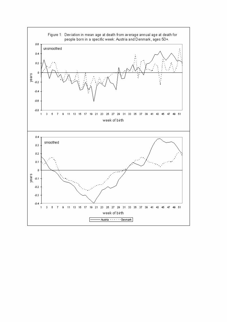
3 ResultsIn the Austrian data set, death after age 50 occurred at an average age of 77.7. The

mean life span of people born in specific weeks of the year deviates from this average, and thedeviations vary periodically in a 12-month cycle (Figure. 1). There was no significantdifference in this pattern between men and women. Average age at death is lowest for thoseborn around week 20 and highest for those born around week 46. I found a similar patternwhen I considered deaths after age 70.

Dividing the year into four quarters (weeks 1-13, 14-26, 27-39, and 40-52) I found thatthe deviation in mean age at death is highly significant (p<0.001) for those born in the secondand the fourth quarters. The life span of people born between weeks 14 and 26 is 0.28 ± 0.03years below average; the life span of those born between weeks 40 and 52 is 0.32 ± 0.03 yearsabove average. For all major groups of causes of death including accidents and suicides, meanage at death of those born in the second quarter is significantly lower than that of individualsborn in the fourth quarter (Table 1). As regards suicides the difference can partly be explainedby the seasonal distribution of suicides: in the Austrian data set the number of suicides peaksbetween March and June and is lowest in December. A similar pattern was found by Avalineet al. [2] for France.

In the Danish data set further life expectancy at age 50 is 27.24 years. The average ageat death is lowest around week 18, and it peaks in week 51. As was the case for Austrians, thelife span of Danes born in specific weeks varies periodically around the mean (Fig. 1). Forthose born in the second quarter, life spans are 0.17 years below average; for those born in thefourth quarter they are 0.13 years above average. This difference is statistically significant(Cox-Mantel statistic: p<0.001).

To test whether the season of birth affects survival up to the oldest ages, I comparedthe distribution of birth dates in different age groups. An excess mortality among people bornduring the first part of the year means that with advancing age the proportion of people bornduring the second part of the year will increase. In both countries the distribution changessignificantly with age: at older ages relatively more people celebrate their birthday in thesecond part of the year than at younger ages (Figure. 2a, 3).

In principle, the differences in life expectancy by month of birth could be caused eitherby factors that influence life span at the end of life, or by factors that work at the beginning oflife. Two possible factors that may affect life expectancy at the end of life are the seasonaldistribution of deaths and the “birthday-effect”.

In both Denmark and Austria deaths peak in late winter and are lowest during thesummer. In the Austrian data set the exact dates of death were redistributed such that in eachweek of the year the same number of people died while the rank order of the death-dates

remained unchanged. Despite the transformation of the monthly death distribution, the excessmortality of those born in spring remains (see Figure. 4).

Survival models 1a and 1b estimate the effect of the month of birth corrected for theimpact of the current month. They reveal that differences according to month of birth remain,even when corrected for seasonally changing mortality risks. Neither the correction for periodfactors nor for cohort factors changes the result (Table 2a, 2b). A model which included aninteraction term between cohort and month of birth showed that the principal pattern of excessmortality for people born in spring is present in all cohorts. In particular, nothing unusual wasfound for those cohorts born shortly before or during World War I.

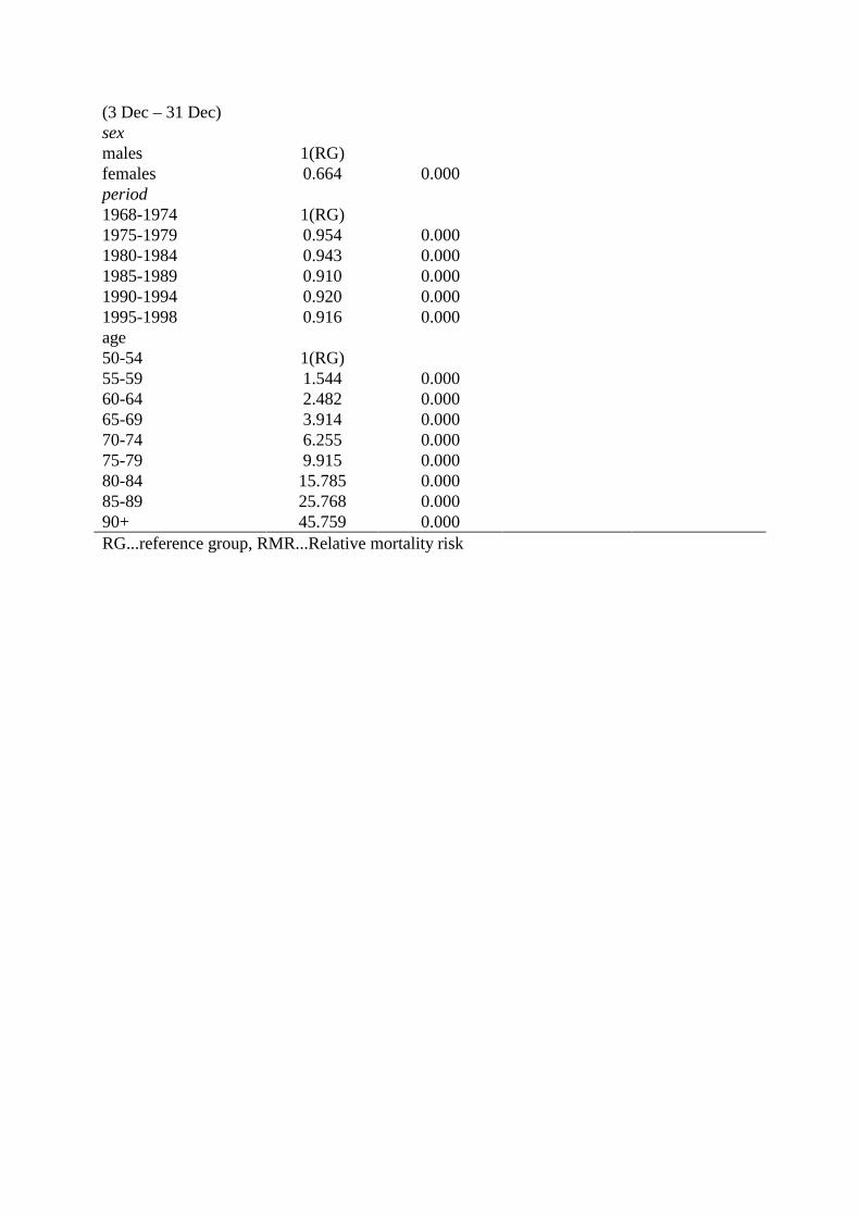
If it is the case that people have a higher risk of death shortly after their birthday, therisk of mortality should be highest in the first three months after their birthday and lowest inthe three months before their next birthday. This pattern should be observed independently ofthe month of birth. The results of the models 2a and 2b (Tables 3a and 3b) show that thoseborn in spring do in fact experience the highest mortality risk within the three months aftertheir birthday. However, those born in autumn and winter tend to have an increased likelihoodto die between four and twelve months after their birthday. This result leads to the conclusionthat there is no “birthday effect” in Denmark. As a consequence the shorter life span of peopleborn in spring is independent of the “birthday effect”.

4 DiscussionThis study is the first comparative analysis of the relationship between month of birth andlongevity on the basis of data for total populations. The life span of 681,677 Austrians and1,371,003 Danes was studied. The Austrian data set is cross-sectional and includes onlyinformation about those who have died but lacks information about the risk-population. Thisis due to the fact that in Austria no population register exists. Therefore, for inter-census yearsit is not possible to sub-divide the Austrian population according to month of birth. Because ofthe restrictions of the Austrian data set I refrained from estimating an event-history modelwhich would be conditional on the outcome of death and would therefore be biased. TheDanish data is based on the population register established in 1968: it is longitudinal andincludes both the population at risk and those who have died. Thus, an event-history model isthe proper statistical method for the analysis of this data.

Both data sets reveal that the mean age at death of people born in spring is lower thanthat of those born in winter. The differences in Austria seem to be greater than in Denmark.Neither the seasonal distribution of deaths nor the ‘birthday effect’ can explain the differencesin life span.

Following I will discuss the evidence for and against three hypotheses that explain therelationship between month of birth and longevity.

The first hypothesis is that the differences in life expectancy are the result of selectivesurvival in infancy. In the last century it was a well-known fact that the likelihood of infants tosurvive their first year of life depended to some extent on their month of birth. Thisknowledge is documented in the extensive data sets on infant mortality in the central statisticaloffices of many countries (for an overview see [6]). Here, there is data on infant mortality bysingle month age groups and by month of death. For example, between 1841 and 1850,Belgian infants born in spring experienced lower mortality during their first three months oflife than infants born in other seasons but were exposed to a greater mortality risk betweentheir third and sixth months [6, 10].

A recent study on infant mortality by age and season of birth [6] shows that for fivecountries in the last century, the mortality risk in the first two years of life differed accordingto the season of birth. The pattern was different in the various countries. The authors explain

this by the interaction between climate and socio-cultural behaviour peculiar to the givencountry, such as breast-feeding and weaning practices. For example, in Italy the summercohorts were advantaged because they went through the summer with the full protectionafforded by breast-feeding and reached winter at an age when they were less vulnerable toviral infections of the respiratory tract. The winter cohorts, on the other hand, were exposed tothe impact of the cold season on respiratory diseases in their first months of life. This was thenfollowed by the hot summers and the accompanying viral infections of the digestive tract, at atime when the protection of breast-feeding was diminished. In Switzerland the pattern was justthe opposite: the mortality risk was highest for those born in spring and summer; it was lowestfor infants born in autumn.

An unpublished analysis of Danish data on infant mortality for the years 1911–1915conducted by the author reveals that in their first year of life, infants who were born in springand early summer had a noticeably increased mortality risk. This pattern runs counter to thenotion that at older ages the difference in life expectancy according to month of birth is due toselective survival during infancy. Selective survival implies that those cohorts live longer thatare born in a season where it is more difficult to survive the first year of life. At older agesthese cohorts will then consist of relatively more robust individuals, since frailer members ofthe cohort already died during infancy. It seems that the opposite is the case: the seasonalpattern in infant death suggests that for those born during the more harmful period of a year,some trait is fixed which makes them more susceptible to diseases later in life.

The explanation of the debilitating effect of early life events, in particular of viralinfections early in life, is supported by a large number of studies on seasonality inschizophrenia. A review by Torrey et al. [19] consists of more than 250 studies covering 29countries in the northern and 5 in the southern hemisphere. For the northern hemisphere mostof these studies find a significant excess of births in winter and spring (December to May) forschizophrenia. A study on schizophrenia in Queensland, Australia, suggests for those born inthe southern Hemisphere an excess birth in their winter (July to September), while those bornin the northern Hemisphere had a March–April birth excess [13]. A recent study in Denmarkon the effects of family history and place and season of birth on the risk of schizophrenia [16]found an excess of spring-births. The authors come to the conclusion that, although in most orall cases genetic factors are a necessary cause of schizophrenia, they are modulated byenvironmental factors such as the season of birth.

The second possible explanation for the differences in life expectancy according tomonth of birth is prenatal influence. A series of studies by Barker (e.g. [4]) suggest that thesusceptibility to circulatory heart diseases later in life may, among other things, also bedetermined by the nutrition of the mother during pregnancy. At the beginning of this centurythe food supply in general, and the availability of fresh fruits and vegetables in particular,differed from season to season. Mothers who gave birth in late autumn and early winter hadaccess to fresh fruits and vegetables throughout most of the time of their pregnancy; those whogave birth in spring and early summer may have experienced relatively longer periods ofinadequate nutrition. However, a study on the effect of the great famine in Finland in the years1866-1868 showed that cohorts born shortly before or during the famine did not have a highermortality risk later in life than those born after the famine [11].

The third hypothesis is that social factors that are closely related to an individual’sbirthday could be responsible for the differences in life span. Age at first school attendance isone example. Children who are born after a certain deadline have to wait one more year beforethey can enrol. In this case they are about a year older than the youngest children in their class.At the turn of the century school started on 1 October in Austria. Those children who had notturned six before this date had to wait another year. Thus, children born in autumn and winter

experienced an age advantage over their classmates who were born at the beginning of theyear. Research suggests that this age advantage affects scholastic aptitude [1, 7, 8] which maytranslate into a lifelong advantage in various ways [18]. However, at the turn of the centurymost schools, especially in rural areas, consisted of only one or two classes. Thus, children ofall ages were instructed together. It is questionable whether a one year age advantage wouldalso influence the development of children in a class where the youngest and the oldest pupilsare more than four years apart in age.

5 ConclusionThis study provides strong evidence that among people aged 50 and older, those born inwinter have a higher life expectancy than those born in summer. This pattern appears not to bethe result of factors that shorten one’s life span at the end of life. It seems rather to result fromfactors that affect individuals early in life. I have raised three hypotheses to explain therelationship between month of birth and longevity. I finally came to the conclusion that atpresent it is not yet known whether the underlying causal mechanisms are of a social or of abiological nature. However, I found evidence that in Denmark selective survival during thefirst year of life cannot explain the observed phenomenon. More insights into the causalmechanisms will be gained by undertaking comparative studies of populations born in thenorthern and the southern hemispheres. In addition, the analysis of seasonal patterns in infantmortality and stillbirths may shed more light on the relationship between month of birth andlife expectancy at older ages.

6 AcknowledgementI am grateful to James W. Vaupel for his comments and suggestions. I thank Josef Kytir,Kaare Christensen, Axel Skytthe and Lisbeth Knudsen for their help in obtaining the data usedin this study, and Jan Hoem and Alexia Prskawetz for their generosity in providing theircomputer codes. I also thank Hans-Georg Müller for his statistical advice.

NotesNote 1.: The following table contains the binary variable sets for the covariates “currentmonth” (v1-v12) and “time lived since last birthday”(p1, p2) for people born in weeks 1-4. Itcan be seen that for a specific month of birth p1 and p2 are always linear combinations of v1to v12. Current month and time lived since last birthday are defined for each year of a person’slive after 1 April 1968. This results in the variables p1 and p2 being highly correlated with thevariables v1 to v12. Ultimately this may be the reason why a model that includes all fourteenvariables simultaneously does not converge.

Current month time livedsince lastbirthday

v1 v2 v3 v4 v5 v6 v7 v8 v9 v10 v11 v12 p1 p20 0 0 0 0 0 0 0 0 0 0 0 0 01 0 0 0 0 0 0 0 0 0 0 0 0 00 1 0 0 0 0 0 0 0 0 0 0 0 00 0 1 0 0 0 0 0 0 0 0 0 1 00 0 0 1 0 0 0 0 0 0 0 0 1 00 0 0 0 1 0 0 0 0 0 0 0 1 00 0 0 0 0 1 0 0 0 0 0 0 1 00 0 0 0 0 0 1 0 0 0 0 0 1 00 0 0 0 0 0 0 1 0 0 0 0 1 00 0 0 0 0 0 0 0 1 0 0 0 1 00 0 0 0 0 0 0 0 0 1 0 0 0 10 0 0 0 0 0 0 0 0 0 1 0 0 10 0 0 0 0 0 0 0 0 0 0 1 0 1

References1. Alton A, Massey A. Date of birth and achievement in GCSE and GCE A-level. EducationalResearch, 1998, 40, 1: 105-109.2. Avaline VF, Baudelot C, Beveraggi M, Lahlou, S. Suicide et rythmes sociaux. Economie etstatistique, 1984, 168: 71-76.3. Barak Y et al. Season of Birth and Autistic Disorder in Israel. Am Journal of Psychiatry,1995, 125, 5: 798-800.4. Barker DJP. Mothers, babies, and disease in later life. 1994, London: BMJ PublishingGroup.5. Bovet J, Spagnoli J, Sudan C. Mortality and birthday. Sozial undPräventivmedizin/Medicine sociale et preventive. 1997, 42, 3: 155-161.6. Breschi M, Bacci ML. Month of birth as a factor in children’s survival. In Desjardins B,Brignoli P, editors. Infant and child mortality in the past. 1997, Oxford. Clarendon press: 157-173.7. Carroll HC. Season of birth and school attendance. British Journal of EducationalPsychology 1992, 62, 3: 391-396.8. Flynn JM, Rahbar MH, Bernstein AJ. Is there an association between season of birth andreading disability? Journal of Developmental and Behavioral Pediatrics 1996, 17, 1:22-26.9. Greville TNE. Short methods of constructing abridged life tables. Rec. Am. Inst. Actuar.1943, 32:29-43.10. Huntington E. Season of birth. 1938, New York: John Wiley and Sons.11. Kannisto V, Christensen K, Vaupel JW. No increased mortality in later life for cohortsborn during famine. Am J Epidemiol. 1997, 11, 145:987-994.12. Lewis MS. Age incidence and schizophrenia: Part I. The season of birth controversy.Schizophrenia Bulletin 1989, 15, 1: 59-73.13. McGrath J, Welham J, Pemberton M. Month of birth, hemisphere of birth andschizophrenia. British Journal of Psychiatry, 1995, 167: 783-785.14. Miura T, Shimura M. Longevity and season of birth(in Jpn., Eng. abs.). Jpn. J.Biometeorology, 1980, 17: 27-31.15.Moore, SE et al. Season of birth predicts mortality in rural Gambia. Nature, 1997, 388:434.16. Mortensen PB et al. Effects of family history and place and season of birth on the risk ofschizophrenia. The New England Journal of Medicine, 1999, 340, 8: 603-608.17. Nakao H, Shimura M, Miura T. Cancers and season of birth - analysis of personal historiesin breast cancer. In Miura T., editor. Seasonality of birth. Progress in Biometeorology, Vol. 6.1987, The Hague: SPB Academic Publishing: 189-196.18. Pflug EJS. Season of birth, schooling and earnings. Targeted Socio-economic Research,Schooling, Training and Transition. 1998, WP- 01-1998: University of Amsterdam.19. Torrey EF, Miller J, Rawlings R, Yolken RH. Seasonality of births in schizophrenia andbipolar disorders: a review of literature. Schizophrenia Research, 1997, 28:1-38.20. Vaupel JW, Yashin AI. Heterogeneity’s ruses: Some surprising effects of selection inpopulation dynamics. The American Statistician, 1985, 39: 176-185.21. Verdoux H. et al. Seasonality of birth in schizophrenia: the effect of regional populationdensity. Schizophrenia Research 1997, 23: 175-180.22. Vézina H. et al. Season of birth and Alzheimer’s disease: a population-based study inSaguenay-Lac-St-Jean/Quebec (IMAGE Project). Psychological Medicine 1996, 26: 143-149.23. Wassermann I, Stack S. Testing the deathdip and deathrise hypothesis: Ohio mortalityresults, 1989-1991. Canadian Studies in Population, 1994, 21,2:133-148.

24. Yuen J. et al. Season of birth and breast cancer risk in Sweden. Br. J. Cancer ,1994, 70:564-568.25. RocaNova Version 2.0 by Sten Martinelle. Copyright Statistics Sweden 1996, PopulationResearch Office.

Table 1: Mean age at death by quarter of birth for major groups of causes of death; all deathsabove age 50 in Austria between the years 1990 and 1997.

Season of birthCause of death 1st

Quarter2nd

Quarter3rd

Quarter4th

QuarterAnnualAverage

p-value(F-test)

Infectious diseases 71.74 71.48 72.39 72.89 72.14 0.314Malignant neoplasm 73.48 73.37 73.56 73.81 73.55 0.000Circulatory diseases 80.26 80.04 80.36 80.64 80.32 0.000Other natural causesof death

77.21 76.76 77.06 77.58 77.20 0.000

Accidents & Suicides 72.77 72.44 72.82 73.31 72.83 0.005

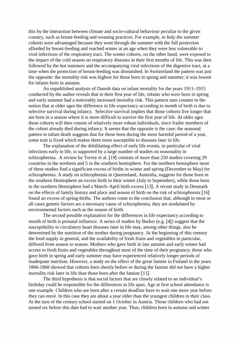
Table 2a: Model 1a: Relative mortality risk estimated by a multivariate survival model whichincludes simultaneously the four covariates “month of birth”, “current month”, “sex” and“period”.

Month of birth Current monthRMR p-value RMR p-value

monthWeeks 1-4(1 Jan –28 Jan)

0.967 0.000 1 (RG)

Weeks 5-8(29 Jan –25 Feb)

0.974 0.000 0.995 0.289

Weeks 9-12(26 Feb – 25 Mar)

0.997 0.542 0.998 0.631

Weeks 13-16(26 Mar – 22 Apr)

1 (RG) 0.998 0.638

Weeks 17-20(23 Apr – 20 May)

1.000 0.836 0.997 0.524

Weeks 21-24(21 May – 17 Jun)

1.002 0.616 0.991 0.046

Weeks 25-28(18 Jun – 15 Jul)

0.994 0.221 0.988 0.012

Weeks 29-32(16 Jul – 12 Aug)

0.981 0.000 0.990 0.026

Weeks 33-36(13 Aug – 9 Sep)

0.979 0.000 0.991 0.060

Weeks 37-40(10 Sep – 7 Oct)

0.974 0.000 0.998 0.640

Weeks 41-44(8 Oct – 4 Nov)

0.971 0.000 0.998 0.683

Weeks 45-48(5 Nov- 2 Dec)

0.969 0.000 1.001 0.834

Weeks 49-52 0.969 0.000 1.001 0.861

(3 Dec – 31 Dec)sexmales 1(RG)females 0.664 0.000period1968-1974 1(RG)1975-1979 0.954 0.0001980-1984 0.943 0.0001985-1989 0.910 0.0001990-1994 0.920 0.0001995-1998 0.916 0.000age50-54 1(RG)55-59 1.544 0.00060-64 2.482 0.00065-69 3.914 0.00070-74 6.255 0.00075-79 9.915 0.00080-84 15.785 0.00085-89 25.768 0.00090+ 45.759 0.000RG...reference group, RMR...Relative mortality risk

Table 2b: Model 1b: Relative mortality risk estimated by a multivariate survival model whichincludes simultaneously the four covariates “month of birth”, “current month”, “sex” and“cohort”.

Month of birth Current monthRMR p-value RMR p-value

monthWeeks 1-4(1 Jan –28 Jan)

0.969 0.000 1 (RG)

Weeks 5-8(29 Jan –25 Feb)

0.976 0.000 0.995 0.289

Weeks 9-12(26 Feb – 25 Mar)

0.998 0.541 0.998 0.631

Weeks 13-16(26 Mar – 22 Apr)

1(RG) 0.998 0.638

Weeks 17-20(23 Apr – 20 May)

1.000 0.865 0.997 0.524

Weeks 21-24(21 May – 17 Jun)

1.000 0.883 0.991 0.046

Weeks 25-28(18 Jun – 15 Jul)

0.993 0.096 0.988 0.012

Weeks 29-32(16 Jul – 12 Aug)

0.980 0.000 0.990 0.026

Weeks 33-36(13 Aug – 9 Sep)

0.977 0.000 0.991 0.060

Weeks 37-40(10 Sep – 7 Oct)

0.971 0.000 0.998 0.640

Weeks 41-44(8 Oct – 4 Nov)

0.968 0.000 0.998 0.683

Weeks 45-48(5 Nov- 2 Dec)

0.965 0.000 1.001 0.834

Weeks 49-52(3 Dec – 31 Dec)

0.964 0.000 1.001 0.861

sexmales 1(RG)females 0.646 0.000cohort1860-1879 1(RG)1880-1889 0.911 0.0001890-1899 0.839 0.0001900-1909 0.782 0.0001910-1918 0.729 0.000age50-54 1(RG)55-59 1.530 0.00060-64 2.370 0.00065-69 3.638 0.00070-74 5.637 0.00075-79 8.742 0.00080-84 13.526 0.000

85-89 21.408 0.00090+ 36.560 0.000RG... reference group, RMR...Relative Mortality Risk

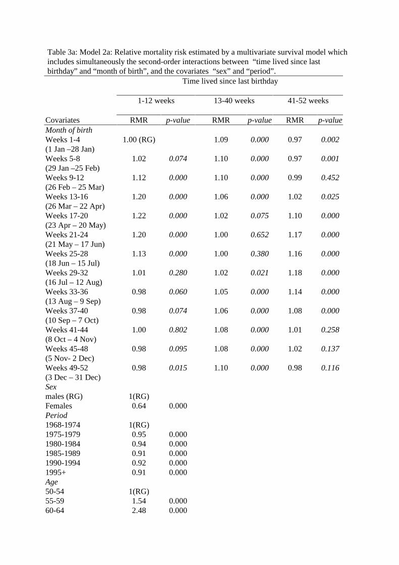
Table 3a: Model 2a: Relative mortality risk estimated by a multivariate survival model whichincludes simultaneously the second-order interactions between “time lived since lastbirthday” and “month of birth”, and the covariates “sex” and “period”.

Time lived since last birthday

1-12 weeks 13-40 weeks 41-52 weeks

Covariates RMR p-value RMR p-value RMR p-valueMonth of birthWeeks 1-4(1 Jan –28 Jan)

1.00 (RG) 1.09 0.000 0.97 0.002

Weeks 5-8(29 Jan –25 Feb)

1.02 0.074 1.10 0.000 0.97 0.001

Weeks 9-12(26 Feb – 25 Mar)

1.12 0.000 1.10 0.000 0.99 0.452

Weeks 13-16(26 Mar – 22 Apr)

1.20 0.000 1.06 0.000 1.02 0.025

Weeks 17-20(23 Apr – 20 May)

1.22 0.000 1.02 0.075 1.10 0.000

Weeks 21-24(21 May – 17 Jun)

1.20 0.000 1.00 0.652 1.17 0.000

Weeks 25-28(18 Jun – 15 Jul)

1.13 0.000 1.00 0.380 1.16 0.000

Weeks 29-32(16 Jul – 12 Aug)

1.01 0.280 1.02 0.021 1.18 0.000

Weeks 33-36(13 Aug – 9 Sep)

0.98 0.060 1.05 0.000 1.14 0.000

Weeks 37-40(10 Sep – 7 Oct)

0.98 0.074 1.06 0.000 1.08 0.000

Weeks 41-44(8 Oct – 4 Nov)

1.00 0.802 1.08 0.000 1.01 0.258

Weeks 45-48(5 Nov- 2 Dec)

0.98 0.095 1.08 0.000 1.02 0.137

Weeks 49-52(3 Dec – 31 Dec)

0.98 0.015 1.10 0.000 0.98 0.116

Sexmales (RG) 1(RG)Females 0.64 0.000Period1968-1974 1(RG)1975-1979 0.95 0.0001980-1984 0.94 0.0001985-1989 0.91 0.0001990-1994 0.92 0.0001995+ 0.91 0.000Age50-54 1(RG)55-59 1.54 0.00060-64 2.48 0.000

65-69 3.91 0.00070-74 6.26 0.00075-79 9.92 0.00080-84 15.79 0.00085-89 25.77 0.00090+ 45.76 0.000RG.......reference group, RMR... Relative Mortality Risk

Table 3b: Model 2b: Relative mortality risk estimated by a multivariate survival model whichincludes simultaneously the second-order interactions between “time lived since lastbirthday” and “month of birth”, and the covariates “sex” and “cohort”.

Time lived since last birthday

1-12 weeks 13-40 weeks 41-52 weeks

Covariates RMR p-value RMR p-value RMR p-valueMonth of birthWeeks 1-4(1 Jan –28 Jan)

1.00 (RG) 1.09 0.000 0.97 0.001

Weeks 5-8(29 Jan –25 Feb)

1.02 0.074 1.10 0.000 0.97 0.001

Weeks 9-12(26 Feb – 25 Mar)

1.12 0.000 1.10 0.000 0.99 0.460

Weeks 13-16(26 Mar – 22 Apr)

1.19 0.000 1.06 0.000 1.02 0.030

Weeks 17-20(23 Apr – 20 May)

1.21 0.000 1.02 0.091 1.10 0.000

Weeks 21-24(21 May – 17 Jun)

1.20 0.000 1.00 0.539 1.16 0.000

Weeks 25-28(18 Jun – 15 Jul)

1.13 0.000 1.00 0.593 1.16 0.000

Weeks 29-32(16 Jul – 12 Aug)

1.01 0.345 1.02 0.069 1.18 0.000

Weeks 33-36(13 Aug – 9 Sep)

0.98 0.037 1.04 0.000 1.13 0.000

Weeks 37-40(10 Sep – 7 Oct)

0.98 0.020 1.06 0.000 1.07 0.000

Weeks 41-44(8 Oct – 4 Nov)

0.99 0.347 1.08 0.000 1.01 0.454

Weeks 45-48(5 Nov- 2 Dec)

0.98 0.019 1.08 0.000 1.01 0.458

Weeks 49-52(3 Dec – 31 Dec)

0.97 0.002 1.09 0.000 0.98 0.019

Sexmales (RG) 1(RG)females 0.65 0.000cohort1860-1879 1(RG)1880-1889 0.91 0.0001890-1899 0.84 0.0001900-1909 0.78 0.0001910-1918 0.73 0.000age50-54 1(RG)55-59 1.53 0.00060-64 2.37 0.000

65-69 3.64 0.00070-74 5.63 0.00075-79 8.73 0.00080-84 13.54 0.00085-89 21.37 0.00090+ 36.50 0.000RG...reference group, RMR... Relative Mortality Risk