Longevity and Lifetime Labor Supply: Evidence and...

Electronic copy available at: http://ssrn.com/abstract=941936

Longevity and Lifetime Labor Supply:

Evidence and Implications∗

Moshe Hazan†

Hebrew University and CEPR

May 19, 2009

Abstract

Conventional wisdom suggests that increased life expectancy had a keyrole in causing a rise in investment in human capital. I incorporate the re-tirement decision into a version of Ben-Porath’s (1967) model and find thata necessary condition for this causal relationship to hold is that increasedlife expectancy will also increase lifetime labor supply. I then show that thiscondition does not hold for American men born between 1840 and 1970 andfor the American population born between 1890 and 1970. The data suggestsimilar patterns in Western Europe. I end by discussing the implications ofmy findings for the debate on the fundamental causes of long-run growth.

JEL Classification: E20, J22, J24, O11.Keywords: Longevity, Hours Worked, Human Capital, Economic Growth.

∗I thank Steven Berry, the co-editor, and four referees for detailed and valuable comments. I also thank DaronAcemoglu, Stefania Albanesi, Mark Bils, Hoyt Bleakley, Matthias Doepke, Reto Foellmi, Oded Galor, Eric Gould, Pe-ter Howitt, Charles Jones, Sebnem Kalemli-Ozcan, Todd Kaplan, Peter Klenow, Kevin Lang, Doron Kliger, Robert Margo,Joram Mayshar, Omer Moav, Joel Mokyr, Dilip Mookherjee, Andy Newman, Claudia Olivetti, Daniele Paserman, ValerieRamey, Yona Rubinstein, Eytan Sheshinski, Avi Simhon, Guillaume Vandenbroucke, David Weil, Joseph Zeira, StephenZeldes, Fabrizio Zilibotti, Hosny Zoabi, conference participants in the Minerva DEGIT, Jerusalem 2006; Society for Eco-nomic Dynamics, Vancouver 2006; NBER Summer Institute, Growth Meeting 2006; European Growth and Integrationsince the Mid-Nineteenth Century (Marie Curie Research Training Network), Lund 2006; The European Meeting of theEconometric Society, Milan 2008; Rags to Riches, Barcelona 2008 and seminar participants at Bar Ilan University, BostonUniversity, Brown University, Columbia University, the University of Cyprus, Haifa University, Hebrew University, Uni-versitat Pompeu Fabra and the University of Zurich. Amnon Schreiber and Shalva Zonenashvili provided excellentresearch assistance. Financial support from the Hebrew University is greatly acknowledged.

†Address: Department of Economics, The Hebrew University of Jerusalem, Mt. Scopus, Jerusalem 91905, Israel.E-mail: [email protected]

Electronic copy available at: http://ssrn.com/abstract=941936

1 Introduction

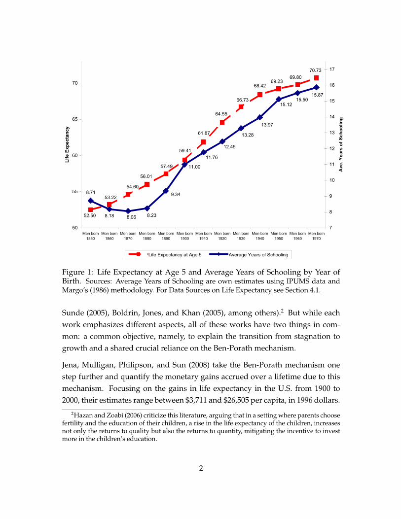
The life expectancy at age 5 of American men born in the mid 19th century was52.5 years and their average years of schooling were less than 9. Their peers, borna hundred years later, gained more than 16 years of life and invested 6 more yearsin schooling (see Figure 1). Conventional wisdom suggests that these gains in lifeexpectancy positively affected schooling by increasing the horizon over whichinvestments in schooling have been paid off. Hereafter, I refer to this mechanismas the Ben-Porath mechanism, following the seminal work of Ben-Porath (1967).1

Prominent scholars have emphasized that in the context of economic growth,exogenous reductions in mortality rates were crucial in initiating the process ofhuman capital accumulation, which itself was instrumental in the transition from“stagnation” to “growth”. For example, Galor and Weil (1999) write,

[. . . ] A second effect of falling mortality is that it raises the rate of return

on investments in a child’s human capital and thus can induce households

to make quality-quantity trade-offs. This inducement to increased invest-

ment in child quality would be complementary to the increase in the rate

of return to human capital discussed in Section 1. [. . . ] The effect of lower

mortality in raising the expected rate of return to human capital investments

will nonetheless be present, leading to more schooling and eventually to a

higher rate of technological progress. This will in turn raise income and fur-

ther lower mortality. (p.153)

This mechanism has been explored theoretically by others as well (see Meltzer(1992), de la Croix and Licandro (1999), Kalemli-Ozcan, Ryder, and Weil (2000),Boucekkine, de la Croix, and Licandro (2002, 2003), Soares (2005), Cervellati and

1The essence of the Ben-Porath model is that individuals choose their human capital accordingto the future rewards that this human capital will receive. The mechanism described above andlabeled “the Ben-Porath mechanism” is one of but several predictions of the Ben-Porath modeland the aim of the current paper is the empirical evaluation of only this prediction. Anotherprominent prediction of the Ben-Porath model suggests that an increase in the rental rate onhuman capital will increase future rewards to human capital and hence increase investment inschooling. This prediction is discussed in the concluding remarks.

1

61.87

66.73

70.73

69.8069.23

68.42

59.41

52.50

53.22

54.60

56.01

57.49

64.55

8.18 8.06 8.23

9.34

11.00

11.76

12.45

13.28

13.97

15.1215.50

15.87

8.71

50

55

60

65

70

Men born

1850

Men born

1860

Men born

1870

Men born

1880

Men born

1890

Men born

1900

Men born

1910

Men born

1920

Men born

1930

Men born

1940

Men born

1950

Men born

1960

Men born

1970

Lif

e E

xp

ecta

ncy

7

8

9

10

11

12

13

14

15

16

17

Ave.

Years

of

Sch

oo

lin

g

Life Expectancy at Age 5 Average Years of Schooling

Figure 1: Life Expectancy at Age 5 and Average Years of Schooling by Year ofBirth. Sources: Average Years of Schooling are own estimates using IPUMS data andMargo’s (1986) methodology. For Data Sources on Life Expectancy see Section 4.1.

Sunde (2005), Boldrin, Jones, and Khan (2005), among others).2 But while eachwork emphasizes different aspects, all of these works have two things in com-mon: a common objective, namely, to explain the transition from stagnation togrowth and a shared crucial reliance on the Ben-Porath mechanism.

Jena, Mulligan, Philipson, and Sun (2008) take the Ben-Porath mechanism onestep further and quantify the monetary gains accrued over a lifetime due to thismechanism. Focusing on the gains in life expectancy in the U.S. from 1900 to2000, their estimates range between $3,711 and $26,505 per capita, in 1996 dollars.

2Hazan and Zoabi (2006) criticize this literature, arguing that in a setting where parents choosefertility and the education of their children, a rise in the life expectancy of the children, increasesnot only the returns to quality but also the returns to quantity, mitigating the incentive to investmore in the children’s education.

2

The Ben-Porath mechanism, however, is not just a legacy of the past. In the con-text of comparative development, several scholars, using different tools, havetried to evaluate the causal effect of life expectancy on investment in humancapital. Acemoglu and Johnson (2006) and Lorentzen, McMillan, and Wacziarg(2008) find no effect of life expectancy on school enrolment using cross countryregressions, whereas Bils and Klenow (2000) and Manuelli and Seshadri (2005)find positive effects, although of a different order of magnitude, using calibratedgeneral equilibrium models.3 The causal effect of life expectancy on investmentin human capital is studied in the development literature as well. Jayachandranand Lleras-Muney (2009) find significant effect of a decline in maternal mortal-ity risk on female literacy rates and school enrolment in Sri Lanka, and Fortson(2007) finds a large negative effect of regional HIV prevalence on individual hu-man capital investment in sub-Saharan Africa.

Finally, the Ben-Porath mechanism is also mentioned outside the academic realm.In the public debate on the benefits of improving health in developing countries,a popular view suggests that while improving the health and longevity of thepoor is an end in itself, it is also a means to achieving economic development.This view is best reflected in the report of the World Health Organization’s Com-mission on Macroeconomics and Health (2001) that states,

The gains in growth of per capita income as a result of improved health are

impressive, but tell only a part of the story. Even if per capita economic

growth were unaffected by health, there would still be important gains in

economic well-being from increased longevity. [. . . ] Longer-lived house-

holds will tend to invest a higher fraction of their incomes in education and

financial saving, because their longer time horizon allows them more years

to reap the benefits of such investments (p. 25).

Despite its popularity, the evidence on the Ben-Porath mechanism is brief andmixed, and encompasses the experience of only recent decades. My purpose isto investigate empirically the relevance of this mechanism to the transition fromstagnation to growth of today’s developed countries.

3See also Caselli (2005) and Ashraf, Lester, and Weil (2008). Both works present calibratedvalues for the elasticity of human capital with respect to the adult mortality rate. The former usescross country data and the latter use micro estimates.

3

I do so by noting that there is a fundamental asymmetry between providing sup-port for a hypothesis and refuting it. While meeting a necessary condition is onlya prerequisite for providing supportive evidence for a hypothesis, failure to meeta necessary condition is sufficient to refute one. I examine therefore a crucialimplication of the Ben-Porath mechanism. Specifically, I argue that although theBen-Porath mechanism is phrased as the effect of the prolongation of (working)life, it in fact suggests that as individuals live longer, they invest more in humancapital, if and only if, their lifetime labor supply increases. Importantly, incorpo-ration of the retirement choice into a version of Ben-Porath’s (1967) model doesnot change the above statement.4 Section 2 of the paper formulates this argu-ment. Clearly, this statement is true as long as schooling is desired only in orderto increase labor market productivity. In Section 9 I discuss several other mo-tives that may positively affect the investment in human capital in response to anincrease in longevity.

The discussion above suggests that the necessary condition for the Ben-Porathmechanism can be tested directly, by looking at the correlation between longevityand lifetime labor supply. I therefore suggest estimating the empirical counter-part of the lifetime labor supply, i.e., the expected total working hours over a life-time (henceforth: ETWH) of consecutive cohorts of American men, born between1840 and 1970 and of all American individuals born between 1890 and 1970. Apositive correlation between ETWH and longevity should serve as supportiveevidence for the Ben-Porath mechanism. Conversely, a negative correlation be-tween these two variables would suggest that the Ben-Porath mechanism cannotaccount for any of the immense increase in education that has accompanied thegrowth process over the last 150 years.

The ETWH is determined by three factors: the age specific mortality rates, whichdetermine the probability of being alive at each age, and the labor supply deci-sions along both the extensive and intensive margins at each age. Clearly, holdinglabor supply decisions constant, the Ben-Porath mechanism suggests a positiveeffect of longevity on lifetime labor supply and thereby on investment in educa-

4An earlier version of this paper, (Hazan 2006), showed that incorporation of a leisure choicedoes not change the statement made above.

4

tion.5 However, the data suggest that the reduction in labor supply along boththe extensive and intensive margins outweighs the gains in longevity, leading toa decline in lifetime labor supply. Thus, if one attempts to decompose the ob-served change in schooling over the relevant period to its different sources, thetotal effect of the Ben-Porath mechanism enters with a non-positive sign, and ittherefore cannot provide an explanation for the observed rise in education.

My approach has two major advantages. Firstly, it relies on sound theoreticalprediction and therefore the empirical test is not specific to econometric speci-fications or structural assumptions. Secondly, it uses the experience of today’sdeveloped countries over more than 150 years and can therefore shed light onthe long-run economic consequences of the prolongation of life in the develop-ing world.

The rest of the paper is organized as follows. In Section 2 I present a simplifiedversion of the Ben-Porath model to explicitly derive the effect of an increase inlife expectancy on education and lifetime labor supply. In Section 3 I present mymethodology for the estimation of the ETWH and in Section 4 I describe the data.In Section 5 I present my results for men and in Section 6 I present results for allindividuals by combining the labor supply of both men and women. In Section 7I explore the robustness of the results and in Section 8 I provide suggestive evi-dence that my results are not confined to the U.S. but are a robust feature of thegrowth process in nineteenth and twentieth centuries. In Section 9 I discuss thebroader implications of my findings and present some concluding remarks.

2 A Prototype of the Ben-Porath Model

In this section I present a simplistic version of the Ben-Porath model. The pur-pose of this section is to explicitly emphasize the implications of this type ofmodel for the effect of an increase in longevity on lifetime labor supply and

5This is the partial, casual effect of life expectancy on education which the literature aims toestimate. See e.g., Acemoglu and Johnson (2006), Lorentzen, McMillan, and Wacziarg (2008) andJayachandran and Lleras-Muney (2009).

5

thereby on investment in schooling.6

Denote consumption at age t by c(t) and let the utility from consumption, u(c),be twice continuously differentiable, strictly increasing and strictly concave. As-sume that labor supply is indivisible so the individual may either be fully em-ployed or retired. Disutility of work, f(t), is independent of consumption andincreases in age, f ′(t) > 0.7 The individual works until retirement, R, and livesuntil T , R ≤ T . This structure implies that the individual’s lifetime utility, V isgiven by:

V =

∫ T

0

e−ρtu(c(t))dt−∫ R

0

e−ρtf(t)dt,

where ρ is the subjective discount rate.

The individual’s productivity during the working period is assumed to be equalto his human capital h. The latter is determined by the individual’s choice ofthe length of the schooling period, s, and the human capital production function,h(s) = eθ(s). Finally, schooling occurs prior to entering the labor market and thesole cost of schooling is foregone earnings. The budget constraint of the individ-ual is then given by:

∫ R

s

e−rteθ(s)dt =

∫ T

0

e−rtc(t)dt, (1)

where r is the interest rate.

Define the Lagrangian associated with maximizing lifetime utility V , subject tothe budget constraint, (1), and let λ be the Lagrange multiplier associated withthis problem. The first order conditions with respect to c(t), R and s are, respec-tively:

e−ρtu′(c(t)) = λe−rt,

6The Ben-Porath model allows for continuing investment in human capital during the phase ofworking life. My simplistic variant of the model does not allow for that. Modeling the schoolingdecision as in Ben-Porath (1967) will complicate the model, making the derivation of lifetimelabor supply analytically intractable. I conjecture, nevertheless, that the results derived in thissection would hold under the more realistic structure of the original Ben-Porath model.

7This is a conventional way to model the retirement motive. See, for example, Sheshinski(2008) and Bloom, Canning, and Moore (2007).

6

e−rs+θ(s) ≥∫ R

s

e−rt+θ(s)θ′(s)dt, (2)

and,e−ρRf(R) ≤ λe−rReθ(s). (3)

To illustrate the relationship between lifetime labor supply and investment in hu-man capital in the most transparent way, I make two simplifying assumptions.Firstly, I assume that r = ρ. This assumption ensures that consumption is con-stant throughout the individual’s life. This property is warranted because theBen-Porath mechanism is silent with respect to life-cycle considerations of con-sumption. Secondly, I concentrate on an interior solution for the schooling andretirement choices. This implies that both (2) and (3) hold with strict equality.8

Using the budget constraint, the optimal consumption becomes:

c = c(s,R) =eθ(s)(e−rs − e−rR)

1− e−rT(4)

and (2) and (3) can be re-written respectively as:

1

θ′(s)=

1− e−r(R−s)

r(5)

and,f(R) = u′(c(s,R))eθ(s). (6)

Note that the left hand side of (5) is the cost to increase schooling to the pointwhere productivity rises by one unit, while the right hand side of (5) is the dis-counted value of an increase in income by one unit per period over the produc-tive life, R − s. Similarly, the left hand side of (6) is the disutility from work atage R, while the right hand side of (6) is the marginal cost of retiring, measuredin terms of the loss of utility from foregone consumption.

Inspection of (4), (5) and (6) reveals the effect of longevity on the optimal levelof schooling, s and lifetime labor supply, R − s. This effect is summarized in the

8Sufficient conditions for an interior solution for R are f(0) = 0 and f(T ) = ∞.

7

following two propositions. The proofs are relegated to the appendix.

Proposition 1 If θ(·) is twice continuously differentiable, strictly increasing and strictlyconcave, an increase in longevity induces an increase in schooling and in lifetime laborsupply.

Proposition 2 If θ(·) is linear, an increase in longevity induces an increase in schoolingand has no effect on lifetime labor supply.

It follows that if there are no diminishing returns to schooling, changes in longevitypositively affect schooling but leave the optimal lifetime labor supply unaffected.Hall and Jones (1999) and Bils and Klenow (2000) argue that in a cross section ofcountries there are sharp diminishing returns to human capital.9 In contrast, thetypical finding in studies based on micro data within countries is that of linearreturns to education. Some argue, however, that the latter studies are more proneto ability bias, which may drive the estimates toward linearity (Card 1995, e.g.).Assuming that the returns to education are (weakly) concave, the effect of anincrease in longevity on lifetime labor supply that increases human capital in-vestment, is non-negative.

I conclude from Propositions 1 and 2 that for any reasonable human capital pro-duction function, a rise in longevity that induces an increase in the investment inhuman capital must also induce a rise in lifetime labor supply. It should be men-tioned that in an earlier version of this paper, (Hazan 2006), the intensive marginof the labor supply decision was modeled and the results with respect to the ef-fect of longevity on schooling and lifetime labor supply were similar to thosesummarized in Propositions 1 and 2. I now proceed with my empirical exerciseof estimating the ETWH of consecutive cohorts of Americans to see whether theirexpected lifetime labor supply has indeed increased in parallel to the increase intheir longevity and schooling, as the Ben-Porath mechanism predicts.

9Most models which analyze long-run growth assume that human capital is strictly increasingand strictly concave with respect to time invested (see Galor and Weil (2000), Kalemli-Ozcan, Ry-der, and Weil (2000), Hazan and Berdugo (2002) and Moav (2005), among others). The assumptionthat θ(·) is strictly increasing and strictly concave implies that the rate of return is diminishing, aless restrictive assumption.

8

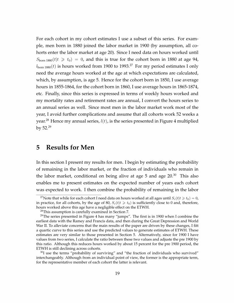
3 Methodology

In this section, I explain my methodology for estimating the ETWH of each co-hort. Let TWHc denote the lifetime working hours of a representative memberof cohort c. Then ETWHc is an average of working hours at each age t, lc(t),weighted by the probability of remaining in the labor market at each age, thesurvivor function, denoted by Sc(t). The ETWH depends, of course, on the age atwhich expectations are calculated. Formally, the ETWH of an individual aged t0

who belongs to cohort c is:

E(TWHc|t > t0) =∞∑

t=t0

lc(t)Sc(t|t > t0).

Below I explain how I estimate the survivor function, Sc(t|t > t0) and then dis-cuss how I deal with the manner in which individuals form their expectationswith respect to the relevant variables that determine the ETWH.

3.1 The Survivor Function

To estimate the survivor function, Sc(t|t > t0), I estimate the hazard function, i.e.,the rate of leaving the labor market in the age interval [t, t + 1), and then cal-culate the survivor function directly. Two factors affect this hazard function: (i)mortality rates–at each age individuals may die and leave the labor market, and(ii) retirement rates–conditional on being alive, at each age individuals choosewhether to continue working or to permanently leave the labor market and re-tire. Specifically, an individual of cohort c who survives to age t0 and is still aliveat age t, leaves the labor market if he dies in the age interval [t, t + 1), an eventthat occurs with probability qc(t). If he remains alive, an event that occurs withprobability 1 − qc(t), he may choose to retire with probability Rc(t). Applyingthe law of large numbers, it follows that the hazard function for the representativemember of cohort c is given by:

λc(t) = qc(t) + (1− qc(t)) ·Rc(t), (7)

9

where qc(t) and Rc(t) are now interpreted as the mortality rate and the retirementrate of the representative member of cohort c at age t, respectively. Hence, toestimate the hazard function using (7), I need data on mortality and retirementrates for each cohort c at each age t, t > t0 . Finally, the survivor function, Sc(t|t >t0) is given by:

Sc(t|t > t0) =t∏

i=t0

(1− λc(i)) . (8)

3.2 The Formation of Expectations

It is important to understand how individuals form expectations regarding mor-tality rates, retirement rates and the hours they intend to work over the courseof their lives, because most of the investment in human capital predates entry tothe labor market. Specifically, I am interested in the way each cohort anticipatesits mortality rate at each age, qc(t), its retirement rate at each age, Rc(t), and thehours it intends to work at each age, lc(t). At one extreme, one can assume thateach cohort perfectly foresees its course of life and hence use the actual mortalityrates, retirement rates and hours worked of cohort members at each age. I referto these estimates as cohort estimates. At the other extreme, one can assume thateach cohort has static expectations and hence use mortality rates, retirement ratesand hours worked by age from the cross section at the age at which expectationsare formed. I refer to these estimates as period estimates. I estimate the ETWHusing these two extreme assumptions, assuming that individuals’ beliefs aboutthe future are a weighted average of these two extremes.

4 Data

As suggested in Section 3, to estimate the ETWH I need data on three variables:the expected mortality and retirement rates and the expected working hours. Asmentioned in Section 3.2, I need different data for the cohort estimates and theperiod estimates. In particular, since the cohort estimates require the utilization

10

of actual cohort data, I can produce these estimates for cohorts born between 1840and 1930. In contrast, the period estimates require cross-sectional data and henceI have these estimates for cohorts born between 1850 and 1970.10 In what follows,each subsection begins by discussing data sources and a general description ofeach variable. A description of the data for the cohort estimates then follows.11

4.1 Mortality Rates

Generally, there are two types of life tables: period life tables and cohort life ta-bles. A period life table is generated from cross-sectional data. It reports, amongother things, the probability of dying within an age interval in the concurrentlyliving population. A cohort life table, on the other hand, follows a specific cohortand reports, among other things, the probability of dying within an age intervalin that specific cohort. If mortality rates at each age were constant over time, theperiod life table and the cohort life table would coincide. However, if mortalityrates were falling over time, the period life table would underestimate gains inlife expectancy of each cohort. In my estimation, I employ data from cohort lifetables for the cohort estimates and period life tables for the period estimates.

My main source is Bell, Wade, and Goss (1992), who provide both period andcohort life tables from 1900 to 2080.12 For earlier periods, I use period life tablesfrom Haines (1998). Note that one can construct cohort life tables from the periodlife table by culling mortality rates for different ages from different years.

Looking across the cohorts I observe that mortality rates have been declining atall ages for men born in 1840 onward. Since I aim to discover whether individualswere expected to increase or decrease their ETWH and decide on their educationin relation to that, I am interested in mortality rates at the “relevant ages”. Sinceinvestment in formal education does not start prior to age 5, and entrance to the

10More accurately, men born between 1836-45 are referred to as “men born 1840”, men bornbetween 1846-55 are referred to as “men born 1850”, etc.

11For brevity, I niether discuss nor present the data for the period estimates in detail and onlypresent the period estimates of the ETWH. A discussion of these data can be found in Hazan(2006).

12Data for the years 1990-2080 reflect projected mortality.

11

labor market starts, on average, at age 20, I focus on mortality rates, conditionalon surviving to ages 5 and 20.

The available data on mortality can be presented in several ways. One way is touse mortality rates at each age to construct survival curves. These curves showthe percentage of individuals who are still alive at each age. A second way is toestimate the life expectancy. Graphically, this is the area under a survival curve.Below I present summary data of these two approaches.

4.1.1 Mortality Rates - Cohort Estimates for Men Born Between 1840 and 1930

Figure 2 plots the survival curves for men born in 1840, 1880 and 1930 who sur-vived to age 20.13 As can be seen from the figure, survival to each age has beenincreasing, with the largest gains concentrated in the ages 50 to 75. These gainsare translated into sizable gains in life expectancy at age 20. While a 20 year-oldman who belongs to the cohort born in 1840 was expected to live for another 43.2years, his counterpart in the cohort born in 1880 was expected to live for another45.65 years and their counterpart born in 1930 was expected to live for another53.01 years. Overall, conditional on surviving to age 20, individuals born in 1930were expected to live almost 10 years more than their counterparts born in 1840.Finally, there were also reductions in mortality rates at younger ages. The prob-ability of surviving to age 20, conditional on being alive at age 5 has increasedfrom 0.92 for individuals born in 1840 to 0.98 for individuals born in 1930, withmost of the increase concentrated in the younger cohorts.14

4.2 Labor Force Participation and Retirement Rates

To estimate retirement rates, I first estimate labor force participation rates andthen compute the retirement rates between age t and age t + 1, Rc(t), as the rate

13Including all ten cohorts on the same graph hides more than it reveals. I choose the cohortborn in 1840 because it is the oldest, the cohort born in 1930 because it is the youngest and thecohort born in 1880 because it is in the middle.

14Figures showing the life expectancy at age 20 and the probability of surviving from age 5 to20 can be found in Hazan (2006).

12

0

0.1

0.2

0.3

0.4

0.5

0.6

0.7

0.8

0.9

1

20 35 50 65 80 95

Age

Fraction

Men born 1840 Men born 1880 Men born 1930

Figure 2: The Probability of Remaining Alive, Conditional on Reaching Age 20for Men Born in 1840, 1880 and 1930: Cohort Estimates. See text for sources.

of change in labor force participation between age t and t + 1.15 To estimate la-bor force participation rates, I use the Integrated Public Use Microdata Series(IPUMS) which are available from 1850 to 2000 (except for 1890) (Ruggles, Sobek,Alexander, Fitch, Goeken, Kelly Hall, King, and Ronnander 2004). Prior to 1940,an individual was considered as part of the labor force if he or she reported hav-ing a gainful occupation. This is also known as the concept of “gainful employ-ment”. From 1940 onward, however, the definition changed and an individualis considered part of the labor force if within a specific reference week, he or shehas a job from which he or she is temporarily absent, working, or seeking work.Some scholars have argued that the former definition is more comprehensive

15Although non-participation at a given age does not necessarily imply permanent retirement,this is what I assume here. This is not a bad assumption since I assume that retirement does notstart prior to age 45. For men age 45 and above, the rate of exit and re-entry to the labor forceis supposedly rather low. Furthermore, if the decision to leave the labor force and then return isuncorrelated across individuals of the same age and cohort, things would average out because Iestimate variables at the cohort level. For expositional purposes, in this section I present the dataon labor force participation rates.

13

than the latter. Moen (1988) suggests a method of estimating a consistent time se-ries of labor force participation rates across all available IPUMS samples, basedon the concept of gainful employment. In my estimation I employ the methodsuggested by Moen.16

4.2.1 Labor Force Participation and Retirement Rates - Cohort Estimates forMen Born Between 1840 and 1930

For each cohort I estimate the labor force participation rate based on the conceptof gainful employment at each age starting from age 45.17 Similar to Figure 2, Fig-ure 3 presents labor force participation rates for men born in 1840, 1880 and 1930.As can be seen, from age 55 and over, the younger the cohort is, the faster the de-cline in its participation. Notice that while participation at age 45 is about 96-97percent for all three cohorts, by age 60 it declines to 89 percent for men born in1840, 80 percent for men born in 1880 and 76 percent for the men in 1930. By age70, the estimates are 61 percent, 48 percent and 29 percent, respectively.18 Thus,while the fraction of those who survive to each age has increased, the fraction ofthose who have already retired has increased as well. In Section 5.1, I combinethe survival and retirement rates to obtain the fraction of those who remain inthe labor market at each age, Sc(t|t > t0).

16See also Costa (1998a), Chapter 2.17I assume that participation rates are constant for all cohorts between age 20 and 45. The data

support this claim firmly. In addition, from age 75 and over, there are too few observations ineach cell. Hence I estimate participation in 5-year intervals (75-9, 80-4, 85-9 and 90-4) and use alinear trend to predict participation at each age. Finally, members of the cohort born in 1920 were84 years old in 2000 and members of the cohort born in 1930 were 74 years old in 2000. Hence forthe cohort born in 1920 I use the participation rates of the cohort born in 1910 at ages 85-94 andfor the cohort born in 1930 I use the participation rates of the cohort born in 1920 at age 75-84 andthe participation rates of the cohort born in 1910 at ages 85-94.

18The long-run decline in labor force participation at age 55 and above is discussed by Costa(1998a) and Moen (1988). Lee (2001) discusses the length of the retirement period of cohorts ofAmerican men born between 1850 and 1990.

14

0.0

0.1

0.2

0.3

0.4

0.5

0.6

0.7

0.8

0.9

1.0

45 55 65 75 85 95

Age

Fraction


Figure 3: Labor Force Participation for Men born in 1840, 1880 and 1930: CohortEstimates. See text for sources.

4.3 Hours Worked

Questions about hours worked last week or usual hours worked per week werenot asked by the U.S. Bureau of the Census prior to 1940. Hence, it is not possibleto estimate a consistent time series of hours worked by age and sex from microdata over my period of interest, 1860-present. Whaples (1990), which is probablythe most comprehensive study on the length of the American work week prior to1900, puts together the available aggregated time-series data from as early as 1830to the present day. Clearly, such series suffer from biases due to the aggregationitself (e.g., changes over time in the workers’ age composition, the fraction ofpart-time workers, the fraction of women in the labor force and so forth), due tosampling of different industries (e.g., manufacturing vs. all private sectors vs. allsectors of the economy) and a host of other reasons.

15

Whaples (1990) reports two time series for the pre 1900 period: the Weeks andthe Aldrich series. The former suggests that the average work week was 62 hoursin 1860, 61.1 hours in 1870 and 60.7 hours in 1880, while the latter suggests thatthe average work week was 66 hours in 1860, 63 hours in 1870, 61.8 hours in 1880and 60 hours in 1890.

During the last quarter of the nineteenth century, state Bureaus of Labor Statis-tics published several surveys of the economic circumstances of non-farm wage-earners. I rely on nine such surveys published between 1888 and 1899, all ofwhich contain information on individuals’ daily hours of work, their wages, ageand sex, as well as other personal characteristics.19 Specifically, I combine thesurveys from California in 1892, Kansas in 1895, 1896, 1897, and 1899, Maine in1890, Michigan stone workers in 1888, Michigan railway workers in 1893 andWisconsin in 1895. Altogether I have data on 13,515 male workers.20 I use thiscombined dataset to generate an estimate of hours worked by males for 1890. Av-erage hours worked by males yields an estimate of 10.2 hours per day, or 61.2 perweek.21 The micro data set allows me to study the distribution of hours workedacross the male population in more detail. The data suggest that average weeklyhours did not vary much by age: although hours are somewhat higher at ages20-29 and 30-39, 61.7 and 61.8 respectively, they were only reduced to 60.2, 60.5,60.3 and 60.2 for the age groups 40-9, 50-9, 60-9 and 70-9, respectively. Across thewage distribution, however, there is more variation. The work week of individ-uals whose wages are in the 10th percentile consisted of 62.15 hours while that ofindividuals whose wages are in the 90th percentile consisted of only 56.53 hours.

Starting in 1900, in contrast, consistent time-series on hours worked both by men,

19The data are available through the Historical Labor Statistics Project, Institute of Businessand Economic Research, University of California, Berkeley, CA 94720. See Carter, Ransom, Sutch,and Zhao (n.d.).

20Costa (1998b) argues that when these data sets are pulled together, they represent quite wellthe occupational distribution of the 1900 census and the 1910 industrial distribution. Hence Iassume that they represent the U.S. population at that time.

21Hours reported in these data sets are per day. As discussed in Costa (1998b), the 1897 Kansasdata set included a question on whether hours worked were reduced or increased on Saturday.Nine percent reported that hours were reduced, 14 percent reported that hours were increasedand 76 percent that they remained the same. Sundstorm (2006) also argues that the typical num-ber of working days per week in the late nineteenth century was 6. Hence, I assume a 6-day workweek.

16

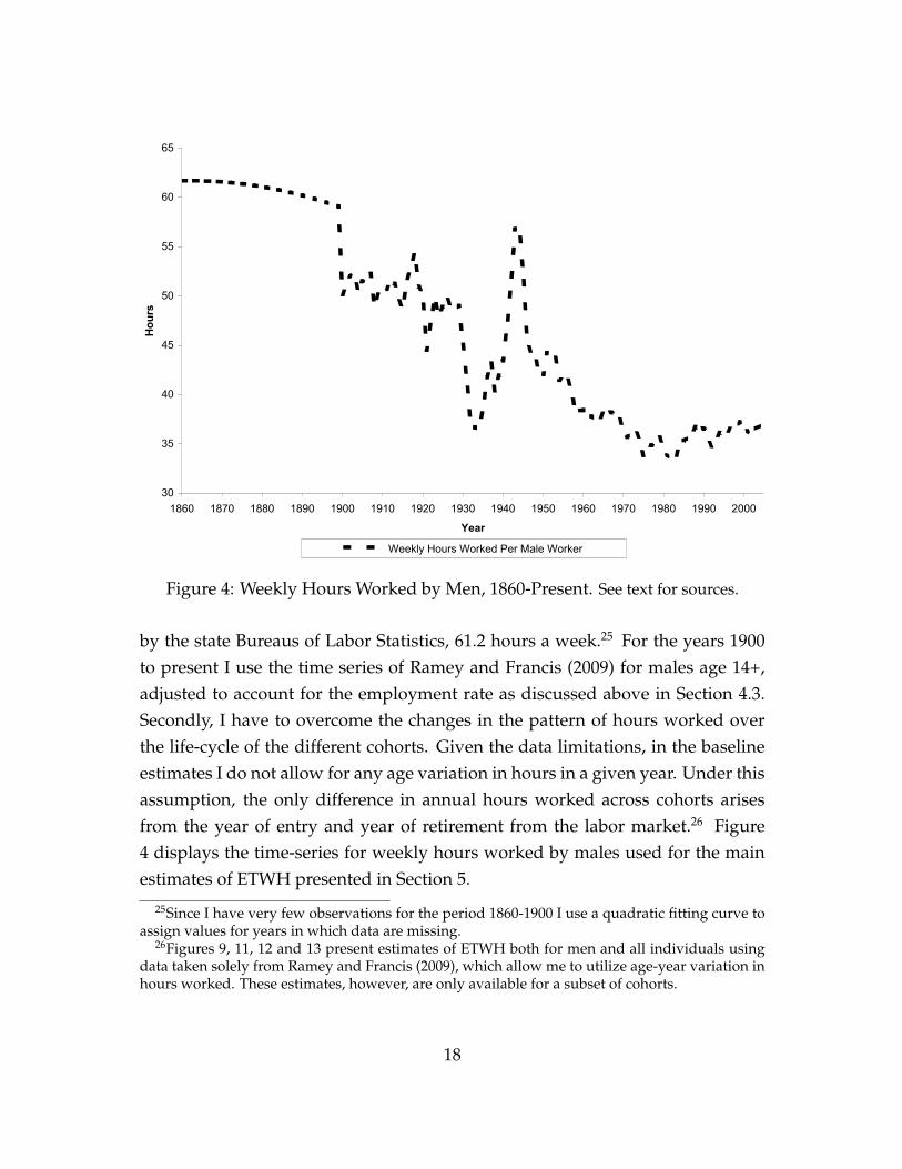
women and all individuals are available from Ramey and Francis (2009), whichare based on Kendrick (1961).22 For my main results of ETWH for men, I usethe time series of hours for males age 14+. These data, however, present hoursworked by person and not per worker. Hence, to transform this data into hoursper worker, I estimate employment rates for males age 14+ from Census dataand divide the hours per person by the fraction of men employed in each year.The resulting time-series suggests that weekly hours per male worker fluctuatedat around 50 hours between 1900 and 1925. It then sharply declined for abouta decade during the Great Depression, rebounded to almost 57 hours a weekduring war time in the years 1943 and 1944, and then started its long run declinefrom about 45 hours a week in 1946 to about 36 hours by 1970. Since then it hasfluctuated at around this value.23

4.3.1 A Baseline Time Series for Hours

The discussion above highlights several obstacles in generating a consistent timeseries of hours worked at each age t for each cohort c. Firstly, in some series thesample consists of men and women while in others it consists only men. Sec-ondly, some series consist of only part of the economy while others report on allsectors of the economy. Thirdly, over time, there is a change in the pattern ofhours worked over a lifetime: in the 1890s and in 1940, hours by age did not varymuch, but starting in 1950, hours by age varied substantially.24 These issues posita problem in generating consistent time series of hours worked by age for eachcohort.

In an attempt to overcome these obstacles, I make the following assumptions.Firstly, for the period 1860-1880, I take the Weeks estimates which are lower thanthe Aldrich estimates for all years: 62 hours in 1860, 61.1 hours in 1870 and 60.7hours in 1880. For 1890, I take my estimate from the micro data sets published

22The data are available athttp://econ.ucsd.edu/˜vramey/research.html/Century_Public_Data.xls

23See also Jones (1963) which documents average weekly hours in manufacturing for the years1900-1957.

24Hazan (2006) presents the cross-sectional relationship between age and hours for variousyears.

17

30

35

40

45

50

55

60

65

1860 1870 1880 1890 1900 1910 1920 1930 1940 1950 1960 1970 1980 1990 2000

Year

Hours

Weekly Hours Worked Per Male Worker

Figure 4: Weekly Hours Worked by Men, 1860-Present. See text for sources.

by the state Bureaus of Labor Statistics, 61.2 hours a week.25 For the years 1900to present I use the time series of Ramey and Francis (2009) for males age 14+,adjusted to account for the employment rate as discussed above in Section 4.3.Secondly, I have to overcome the changes in the pattern of hours worked overthe life-cycle of the different cohorts. Given the data limitations, in the baselineestimates I do not allow for any age variation in hours in a given year. Under thisassumption, the only difference in annual hours worked across cohorts arisesfrom the year of entry and year of retirement from the labor market.26 Figure4 displays the time-series for weekly hours worked by males used for the mainestimates of ETWH presented in Section 5.

25Since I have very few observations for the period 1860-1900 I use a quadratic fitting curve toassign values for years in which data are missing.

26Figures 9, 11, 12 and 13 present estimates of ETWH both for men and all individuals usingdata taken solely from Ramey and Francis (2009), which allow me to utilize age-year variation inhours worked. These estimates, however, are only available for a subset of cohorts.

18

For each cohort in my cohort estimates I use a subset of this series. For exam-ple, men born in 1880 joined the labor market in 1900 (by assumption, all co-horts enter the labor market at age 20). Since I need data on hours worked untilSborn 1880(t|t > t0) = 0, and this is true for the cohort born in 1880 at age 94,lborn 1880(t) is hours worked from 1900 to 1993.27 For my period estimates I onlyneed the average hours worked at the age at which expectations are calculated,which, by assumption, is age 5. Hence for the cohort born in 1850, I use averagehours in 1855-1864, for the cohort born in 1860, I use average hours in 1865-1874,etc. Finally, since this series is expressed in terms of weekly hours worked andmy mortality rates and retirement rates are annual, I convert the hours series toan annual series as well. Since most men in the labor market work most of theyear, I avoid further complications and assume that all cohorts work 52 weeks ayear.28 Hence my annual series, l(t), is the series presented in Figure 4 multipliedby 52.29

5 Results for Men

In this section I present my results for men. I begin by estimating the probabilityof remaining in the labor market, or the fraction of individuals who remain inthe labor market, conditional on being alive at age 5 and age 20.30 This alsoenables me to present estimates on the expected number of years each cohortwas expected to work. I then combine the probability of remaining in the labor

27Note that while for each cohort I need data on hours worked at all ages until Sc(t|t > t0) = 0,in practice, for all cohorts, by the age of 80, Sc(t|t > t0) is sufficiently close to 0 and, therefore,hours worked above this age have a negligible effect on the ETWH.

28This assumption is carefully examined in Section 7.29The series presented in Figure 4 has many “jumps”. The first is in 1900 when I combine the

earliest data with the Ramey and Francis data, and then during the Great Depression and WorldWar II. To alleviate concerns that the main results of the paper are driven by these changes, I fitta quartic curve to this series and use the predicted values to generate estimates of ETWH. Theseestimates are very similar to those presented in Section 5. Alternatively, since for 1900 I havevalues from two series, I calculate the ratio between these two values and adjuste the pre 1900 bythis ratio. Although this reduces hours worked by about 15 percent for the pre 1900 period, theETWH is still declining across cohorts.

30I use the terms “probability of surviving” and “the fraction of individuals who survived”interchangeably. Although from an individual point of view, the former is the appropriate term,for the representative member of each cohort the latter is relevant.

19

0

0.1

0.2

0.3

0.4

0.5

0.6

0.7

0.8

0.9

1

20 25 30 35 40 45 50 55 60 65 70 75 80 85 90 95

Age

Fraction


Figure 5: The Probability of Remaining in the Labor Market, Conditional on En-try into the Labor Force at Age 20: Cohort Estimates for Men. See text for sources.

market with the series of hours worked per year to arrive at my main results, theETWH.

5.1 The Probability of Remaining in the Labor Market - Cohort

Estimates for Men Born 1840–1930

In this section I present my cohort estimates of Sc(t|t > t0), the fraction of indi-viduals who remain in the labor market at age t, conditional on being alive at aget0, for members of cohort c. Specifically, I let t0 = 20 and assume that individu-als of each cohort enter the labor market at age 20. I then estimate the fractionof those who remain in the labor market at all ages over 20, by estimating thehazard function, (7), and computing Sc(t|t > 20) using (8). Figure 5 shows thefraction of individuals who remain in the labor market conditional on being alive

20

35.11 34.96

36.01

37.39

38.11

39.08

40.85

37.4937.77 37.68

38.40

39.59

40.35

41.73

34.26

34.86

38.98

40.32

40.68

37.23

33

34

35

36

37

38

39

40

41

42

Men born

1840

Men born

1850

Men born

1860

Men born

1870

Men born

1880

Men born

1890

Men born

1900

Men born

1910

Men born

1920

Men born

1930

Years

Expected at age 5 Expected at age 20

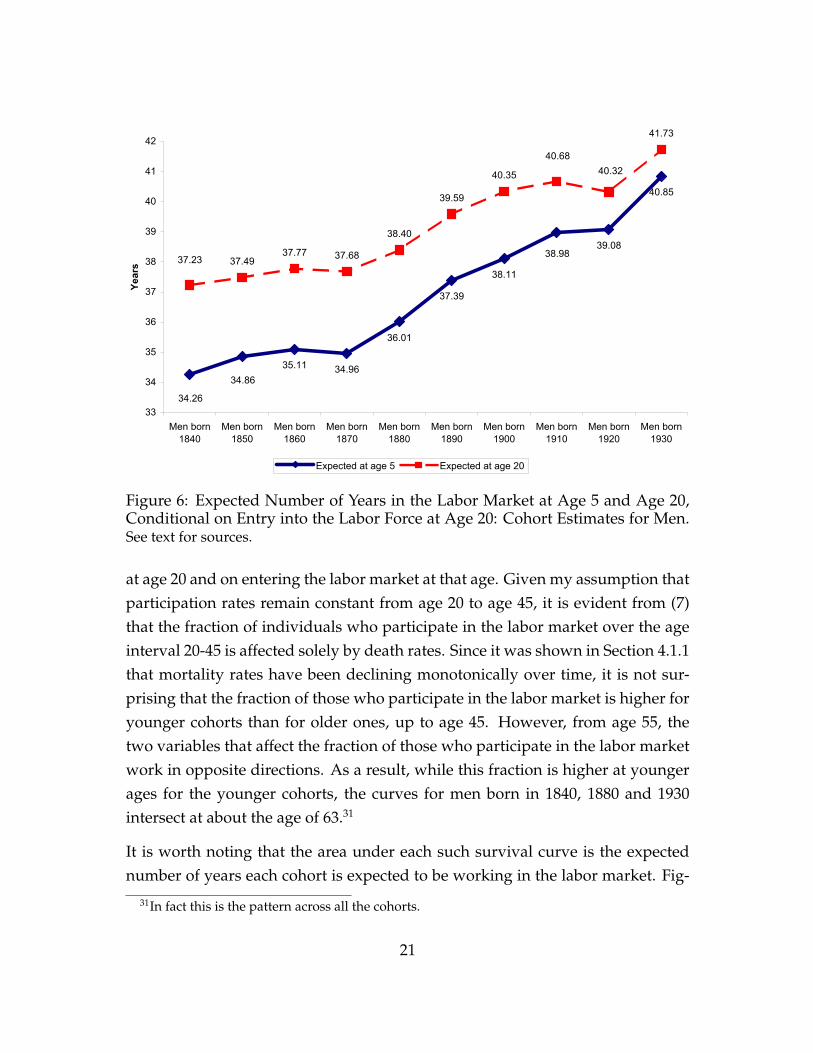
Figure 6: Expected Number of Years in the Labor Market at Age 5 and Age 20,Conditional on Entry into the Labor Force at Age 20: Cohort Estimates for Men.See text for sources.

at age 20 and on entering the labor market at that age. Given my assumption thatparticipation rates remain constant from age 20 to age 45, it is evident from (7)that the fraction of individuals who participate in the labor market over the ageinterval 20-45 is affected solely by death rates. Since it was shown in Section 4.1.1that mortality rates have been declining monotonically over time, it is not sur-prising that the fraction of those who participate in the labor market is higher foryounger cohorts than for older ones, up to age 45. However, from age 55, thetwo variables that affect the fraction of those who participate in the labor marketwork in opposite directions. As a result, while this fraction is higher at youngerages for the younger cohorts, the curves for men born in 1840, 1880 and 1930intersect at about the age of 63.31

It is worth noting that the area under each such survival curve is the expectednumber of years each cohort is expected to be working in the labor market. Fig-

31In fact this is the pattern across all the cohorts.

21

ure 6 plots the number of years that each cohort was expected to work, for indi-viduals who survive to age 20, assuming that entry age is fixed at 20.32 As canbe seen from this figure, the representative member of the cohort born in 1840was expected to work for 37.23 years, whereas his counterpart born in 1930 wasexpected to work for 41.73 years. I then redo this exercise, assuming that expec-tations are calculated at age 5 (i.e., t0 = 5), but maintaining the assumption thatentry to the labor market occurs at age 20. Since the probability of surviving toage 20, conditioned on surviving to age 5, increases across cohorts, the differ-ence in the expected number of years across the cohort is larger by about twoyears. Overall, it is evident that the lower mortality rates for the younger cohortsslightly outweigh their higher retirement rates. Given that the ETWH is an aver-age of the hours worked at each age, weighted by the probability of being in thelabor market at that age, the trend in ETWH across the cohorts at hand will bemostly determined by the trend in hours-worked at each age.

5.2 ETWH: Cohort Estimates

I now present the main results of the paper. Figures 7 and 8 present the cohortestimates of the ETWH for cohorts of men born between 1840 and 1930. Eachfigure contains two series of estimates. The first is labeled “by Age 95” and showsthe ETWH until each cohort is completely retired from the labor market. Thesecond is labeled “by Age 70” and shows the ETWH, truncated at age 70. Thelatter is presented to alleviate any concerns that the declining trend of ETWHmight be driven by men older than 70 years old, who conditional on participatingin the labor market, worked more than 60 hours a week in the late 19th century.33

I begin by presenting the estimates under the assumption that expectations arecalculated at age 20. As can be seen in Figure 7, the lifetime labor supply as mea-

32Note that this is a very conservative assumption. While participation at ages 20-24 is lowerthan at ages 25-45 for the younger cohorts, probably due to college education, for the oldestcohorts, the average age of entrance to the labor market was likely to have been lower than 20.Hence I over-estimate the difference in the expected number of years in the labor market betweenthe oldest and youngest cohorts, which, in turn, under-estimate the difference in ETWH.

33Hereafter, all figures which present estimates of ETWH show both ETWH by age 95 and age70.

22

sured by the ETWH of consecutive cohorts has been declining monotonically.The oldest cohort, born in 1840, was expected to work 115,378 hours in its life-time. In contrast, the youngest cohort, born in 1930, was expected to work only81,411 hours. This amounts to a decline of more than 29 percent between menborn in 1840 and 1930, an average decline of more than 2.5 percent between twoadjacent cohorts.

81,411

112,279

109,298

98,816

93,945 93,581

90,531

86,000

83,194

79,182

85,023

87,692

92,122

95,56296,233

101,271

107,835

112,199

115,378

105,712

75,000

80,000

85,000

90,000

95,000

100,000

105,000

110,000

115,000

120,000

Men born

1840

Men born

1850

Men born

1860

Men born

1870

Men born

1880

Men born

1890

Men born

1900

Men born

1910

Men born

1920

Men born

1930

Hours

Expected Total Working Hours Over the Lifetime at Age 20, by Age 95

Expected Total Working Hours Over the Lifetime at Age 20 by Age 70

Figure 7: Expected Total Working Hours over the Lifetime of Consecutive Co-horts of Men Born Between 1840 and 1930. Individuals Are Assumed to Enterthe Labor Market at Age 20: Cohort Estimates are Calculated at Age 20. See textfor sources and estimation procedure.

The probability of surviving to age 20 from age 5, however, has increased from0.92 for the cohort born in 1840 to 0.98 for the cohort born in 1930. Since in-vestment in education begins at age 5, one might rightfully argue that the ageat which expectations should be calculated is age 5.34 This is what I do in Fig-

34Recall that while expectations are calculated at age 5, it is assumed that the age of entery thelabor market is 20.

23

106,176

104,352

90,245 90,269

87,020

84,039

82,412

79,684

100,217

93,972

80,640

82,417

85,517

88,39888,100

91,694

98,244

101,654

103,324

77,50275,000

80,000

85,000

90,000

95,000

100,000

105,000

110,000

Men born

1840

Men born

1850

Men born

1860

Men born

1870

Men born

1880

Men born

1890

Men born

1900

Men born

1910

Men born

1920

Men born

1930

Hours


Expected Total Working Hours Over the Lifetime at Age 5 by Age 70

Figure 8: Expected Total Working Hours over the Lifetime of Consecutive Co-horts of Men Born Between 1840 and 1930. Individuals Are Assumed to Enterthe Labor Market at Age 20: Cohort Estimates are Calculated at Age 5. See text forsources and estimation procedure.

ure 8. As can be seen, although the difference in the ETWH between the cohortshas narrowed, it is still substantial: while members of the earliest cohort wereexpected at age 5 to work for 106,176 hours over their lifetime, their counterpartsborn ninety years later, were expected at that age to work for 79,684 hours. Thisamounts to a decline of nearly 25 percent between men born in 1840 and 1930,an average decline of more than 2 percent between two adjacent cohorts. Finally,note that in both figures, the decline in ETWH is monotonic across the cohorts.

The main advantage of the estimates presented in Figures 7 and 8 is that theyencompass ten cohorts of men born over a period of ninety years. They suffer,however, from two disadvantages, due to the time-series of annual hours-workedused in the estimation. Firstly, the hours series used for these estimates combinesdifferent sources for the pre 1900 and post 1900 period. Secondly, it does not

24

allow for age-year variation in hours worked. To alleviate concerns that the de-clining trend in ETWH is generated due to potential biases in the time-series ofhours worked used, I employ data on hours worked by men from 1900 to 2005,computed by Ramey and Francis (2009). These data enable me to overcome thetwo shortcomings just mentioned, at the expense of obtaining cohort estimates ofthe ETWH of men born between 1890 and 1930.35 Given that Ramey and Francisreport hours per person by age groups with the youngest age group containingmen aged 10 till 13, I assume that expectations are formed at age 10, and removemy earlier assumption that men of all cohorts enter the labor market at age 20.

Figure 9 presents the cohort estimates of ETWH for men born 1890-1930, usingRamey and Francis’ data.36 A few points are worth mentioning. Firstly, similarto the estimates presented in Figures 7 and 8, ETWH is monotonically decreasingacross cohorts. Secondly, although the estimates based on Ramey and Francis’data are somewhat larger than those presented in Figures 7 and 8, the differ-ence across cohorts is almost constant. Finally, the decline across cohorts doesnot spring from different behavior at very old ages: the difference between theETWH by age 95 and by age 70 is almost constant.

5.3 ETWH: Period Estimates

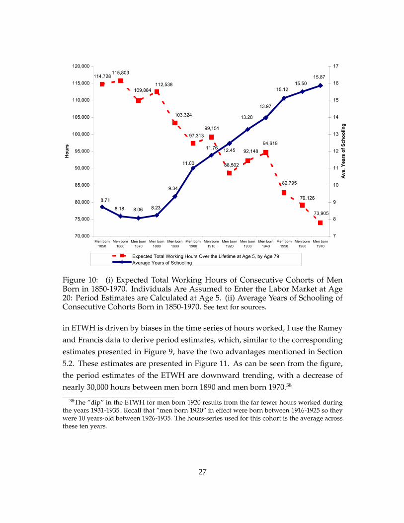
One reason to present the period estimates is that assuming that individuals per-fectly foresee their entire lifetime may be a strong assumption. Hence, I alsopresent the period estimates for ETWH for men born between 1850 and 1970.Figure 10 presents the period estimates for ETWH until age 79, assuming that ex-pectations are taken at age 5.37 While the period estimates series does not mono-

35The Ramey and Francis’ data comprise hours per person and not per worker. I therefore ad-just my methodology such that I define the survivor function as the probability of being alive andweight it by hours worked per person, a series which already takes into account the participationdecision, conditional on being alive.

36Men born 1920 were of age 85 in 2005 and men born 1930 were of age 75 in 2005. I assumethat men born 1920 work the same number of hours at ages 86-95 as men born 1910. Similarly, Iassume that men born 1930 work the same number of hours at ages 75-84 as men born 1920 andthe same number of hours at ages 86-95 as men born 1910.

37The truncation at age 79 is because the period life tables in Haines (1998) do not report thedeath rate for individuals age 80 and over. This is not a major problem, however. Since S(·) is

25

96,593

93,263

89,239

84,968

83,647

98,316

94,602

90,535

86,434

85,534

80,000

82,000

84,000

86,000

88,000

90,000

92,000

94,000

96,000

98,000

100,000

Men born 1890 Men born 1900 Men born 1910 Men born 1920 Men born 1930

Hours



Figure 9: Expected Total Working Hours over the Lifetime of Consecutive Co-horts of Men Born in 1890-1930. Cohort Estimates Calculated at Age 10. Hoursseries based on Ramey and Francis (2008). See text for sources and estimation proce-dure.

tonically decline between each adjacent cohorts, e.g., men born 1850 expectedto work a thousand hours less than men born 1860, the general trend is clear:ETWH declined by more than 35 percent between men born in 1850 and menborn in 1970.

The baseline time series of hours used in these estimates is the one used in thecohort estimates presented in Figures 7 and 8. Note that the nature of the periodestimates exposes them to a larger biases than the cohort estimates, for a givenbias in the hours-series. Hence, to alleviate the concern that the declining trend

non-increasing, and since in the data the older the cohort is, the larger the value of Sc(79), when Iuse Sc(t), t ≤ 79, to estimate the ETWH, I under-estimate the differences across cohorts. Estimatesof the ETWH by age 70 are not presented, for clarity, because their values are very similar to thosepresented here.

26

114,728115,803

97,313

109,884

112,538

103,324

82,795

79,126

94,619

73,905

92,148

88,502

99,151

8.71

8.18 8.06 8.23

9.34

11.00

11.7612.45

13.28

13.97

15.12

15.50

15.87

70,000

75,000

80,000

85,000

90,000

95,000

100,000

105,000

110,000

115,000

120,000

Men born

1850

Men born

1860

Men born

1870

Men born

1880

Men born

1890

Men born

1900

Men born

1910

Men born

1920

Men born

1930

Men born

1940

Men born

1950

Men born

1960

Men born

1970

Ho

urs

7

8

9

10

11

12

13

14

15

16

17

Av

e.

Ye

ars

of

Sc

ho

oli

ng


Average Years of Schooling

Figure 10: (i) Expected Total Working Hours of Consecutive Cohorts of MenBorn in 1850-1970. Individuals Are Assumed to Enter the Labor Market at Age20: Period Estimates are Calculated at Age 5. (ii) Average Years of Schooling ofConsecutive Cohorts Born in 1850-1970. See text for sources.

in ETWH is driven by biases in the time series of hours worked, I use the Rameyand Francis data to derive period estimates, which, similar to the correspondingestimates presented in Figure 9, have the two advantages mentioned in Section5.2. These estimates are presented in Figure 11. As can be seen from the figure,the period estimates of the ETWH are downward trending, with a decrease ofnearly 30,000 hours between men born 1890 and men born 1970.38

38The ”dip” in the ETWH for men born 1920 results from the far fewer hours worked duringthe years 1931-1935. Recall that ”men born 1920” in effect were born between 1916-1925 so theywere 10 years-old between 1926-1935. The hours-series used for this cohort is the average acrossthese ten years.

27

76,261

83,466

87,904

92,805

96,488

89,294

103,802105,767104,885

77,768

85,307

90,474

96,657

100,545

93,596

108,940

110,817109,909

70,000

75,000

80,000

85,000

90,000

95,000

100,000

105,000

110,000

115,000

Men born

1890

Men born

1900

Men born

1910

Men born

1920

Men born

1930

Men born

1940

Men born

1950

Men born

1960

Men born

1970

Hours



Figure 11: Expected Total Working Hours over the Lifetime of Consecutive Co-horts of Men Born in 1890-1970. Individuals Are Assumed to Enter the LaborMarket at Age 20: Period Estimates are Calculated at Age 10. Hours series basedon Ramey and Francis (2009). See text for sources and estimation procedure.

6 Results for All Individuals

Thus far, the estimates presented of ETWH were only for men. One may worry,however, that the focus on men may be biasing the results against the Ben-Porathmechanism. To see why, suppose one tested the theory on women instead. Onewould find that as longevity increased, both education and lifetime labor supplyincreased, thereby supporting the Ben-Porath mechanism. Thus, in this section Ipresent estimates of ETWH for all individuals by combining mortality data andlabor market decisions for both men and women.39

Due to data availability on hours worked by all individuals, however, I can only

39I thank two referees for raising this point and for suggesting that I make use of the Rameyand Francis data to address this issue.

28

63,927

63,128

61,916

61,058

62,342

62,513

61,952

60,711

59,653

60,655

59,000

60,000

61,000

62,000

63,000

64,000

65,000

Individuals born 1890 Individuals born 1900 Individuals born 1910 Individuals born 1920 Individuals born 1930

Hours



Figure 12: Expected Total Working Hours over the Lifetime of Consecutive Co-horts of All Individuals Born in 1890-1930. Cohort Estimates are Calculated atAge 10. See text for sources and estimation procedure.

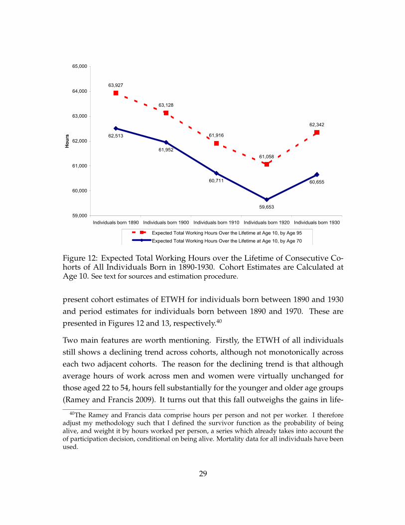
present cohort estimates of ETWH for individuals born between 1890 and 1930and period estimates for individuals born between 1890 and 1970. These arepresented in Figures 12 and 13, respectively.40

Two main features are worth mentioning. Firstly, the ETWH of all individualsstill shows a declining trend across cohorts, although not monotonically acrosseach two adjacent cohorts. The reason for the declining trend is that althoughaverage hours of work across men and women were virtually unchanged forthose aged 22 to 54, hours fell substantially for the younger and older age groups(Ramey and Francis 2009). It turns out that this fall outweighs the gains in life-

40The Ramey and Francis data comprise hours per person and not per worker. I thereforeadjust my methodology such that I defined the survivor function as the probability of beingalive, and weight it by hours worked per person, a series which already takes into account theof participation decision, conditional on being alive. Mortality data for all individuals have beenused.

29

65,570

63,225

65,169

67,457

57,493

61,774

60,523 60,236 60,192

70,651

68,27568,645

60,292

65,963

64,538

62,622

61,84161,503

55,000

57,000

59,000

61,000

63,000

65,000

67,000

69,000

71,000

Individuals

born 1890

Individuals

born 1900

Individuals

born 1910

Individuals

born 1920

Individuals

born 1930

Individuals

born 1940

Individuals

born 1950

Individuals

born 1960

Individuals

born 1970

Hours



Figure 13: Expected Total Working Hours over the Lifetime of Consecutive Co-horts of All Individuals Born in 1890-1970. Period Estimates are Calculated atAge 10. See text for sources and estimation procedure.

expectancy across the cohorts at study. Secondly, in light of the long-run trendof increasing labor supply of women, the decline in ETWH across cohorts is of amuch smaller magnitude, compared to the estimates for men.

7 Robustness of the Results

In this section I explore the robustness of my estimates for the ETWH for men.Some scholars argue that in nineteenth century America, most employment, par-ticularly that in agriculture, was seasonal (Atack and Bateman 1992, Engermanand Goldin 1994). Since seasonality in employment declined over time, my as-sumption that workers of all cohorts work 52 weeks a year biases upward thedifference across cohorts in the ETWH. To explore this possibility I conduct a

30

25.6725.57

26.63

30.45

26.30

30.75

28.77

25

26

27

28

29

30

31

32

Men born 1850 Men born 1860 Men born 1870 Men born 1880 Men born 1890 Men born 1900 Men born 1910

weeks

Figure 14: Counterfactual Experiment: Expected Number of Weeks of Employ-ment that would equalize ETWH to that of the Cohort Born in 1970. See text forthe derivation of these estimates.

counterfactual experiment. I try to answer the hypothetical question: how manyweeks of employment a year does the representative member of the cohorts bornbetween 1850 and 1910 expect to work, such that his ETWH would be equal tothat of the representative member of the cohort born in 1970. I then compare theanswer to the estimates implied by Engerman and Goldin (1994).

In order for the representative member of the cohort born in 1850 to have hisETWH equal that of the representative member of the cohort born in 1970, heshould have expected to work 1,596 hours a year. In 1860, the year at which therepresentative member of the cohort born in 1850 was 10 years old, the weeklyaverage hours of work was 62.17. Hence, to work 1,596 annual hours the repre-sentative member of this cohort should have expected to be employed for about26 weeks a year. The answer for this hypothetical question for all cohorts bornbetween 1850 and 1910 is presented in Figure 14. As can be seen, for all these

31

cohorts, employment of less than 31 weeks a year was enough to expect a life-time labor supply that is equal to that of the cohort born in 1970. Note that thesenumbers imply an expected length of unemployment of almost 5 months a year,which is well above the findings of Engerman and Goldin (1994) and Atack, Bate-man, and Margo (2002). Specifically, Engerman and Goldin find that in 1900 thelength of unemployment, conditional on being unemployed, was between 3 to 4months. Yet, the probability of being unemployed in 1900 was less than 50 per-cent. Taking these two findings together, it follows that the expected months ofunemployment did not exceed 2. Similarly, Atack, Bateman, and Margo (2002)find that the full time equivalent months of employment was nearly 11 months ayear both in 1870 and 1880.

8 The European Experience

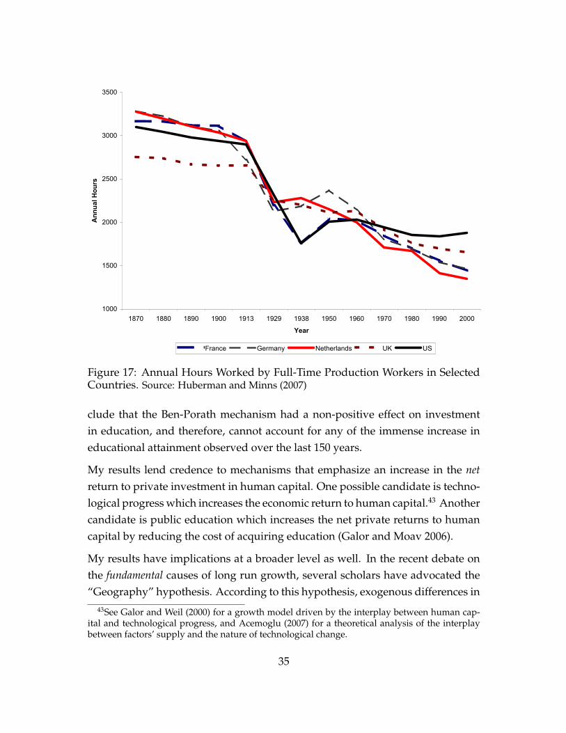
Was the American experience unique? Does the lifetime labor supply of Euro-pean men display a different time trend? In this section I briefly discuss the dataon the determinants of lifetime labor supply in some European countries andcompare them to U.S. data.41 Although the data in this section are somewhatsuggestive, my purpose is to show that my results are not unique to the U.S.experience, but rather a robust feature of the process of development of today’sdeveloped economies. To this end, I present time series of (i) life expectanciesfor males at age 5 (Figure 15), (ii) labor force participation of men aged 65 andover (Figure 16) and (iii) annual hours of work of full-time production workers(Figure 17). Figures 15–17 demonstrate remarkable similarities across these coun-tries in the determinants of ETWH, both in terms of the trends and magnitudes.I therefore conjecture that the decline in ETWH across cohorts is not unique tothe American experience but a robust feature of the process of development intoday’s developed economies.

41The selection of countries reflects availability of data from the various sources used. Refer-ences to the various sources are given in the figures.

32

40

45

50

55

60

65

70

75

1850 1860 1870 1880 1890 1900 1910 1920 1930 1940 1950 1960 1970 1980 1990 2000

Year

Years

France Germany Netherlands UK US

Figure 15: Life Expectancies at Age 5 for Males in Selected Countries, Period LifeTables. Sources: Data for France, Germany, Netherlands and UK are from the HumanMortality Database. Data sources for the U.S. are described in Section 4.1.

9 Concluding Remarks

In this paper, I demonstrate that the commonly utilized mechanism according towhich prolonging the period in which individuals may receive returns on theirhuman capital, spurs investment in human capital and causes growth, has an im-portant implicit implication. Namely, that as life prolongs, lifetime labor supplymust increase as well. Hence, I argue that this mechanism has to satisfy this nec-essary condition. Utilizing data on consecutive cohorts of American men, bornbetween 1840 and 1970, I show that this mechanism fails to satisfy its necessarycondition. Specifically, the estimates of lifetime labor supply, and average yearsof schooling, which are shown together in Figure 10, reject this necessary condi-

33

0

10

20

30

40

50

60

70

80

90

1850 1860 1870 1880 1890 1900 1910 1920 1930 1940 1950 1960 1970 1980 1990

Year

Percent

France Germany UK US

Figure 16: Labor Force Participation of Men Aged 65 and over in Selected Coun-tries. Source: Costa (1998a), Table 2A.2.

tion unequivocally.42 I also provide suggestive evidence that the determinants oflifetime labor supply are remarkably similar between the U.S. and other devel-oped countries, such as England, France, Germany, and the Netherlands. Thus,I conjecture that my main result that ETWH has declined is a robust feature ofthe process of development in today’s developed economies. I therefore con-

42The correlation between the period estimates of ETWH and schooling is -0.93 with a p value of0, and between the cohort estimates of ETWH and schooling is -0.85, with a p value of 0.0081. Onemay argue that hours per school day may have been reduced as well, challenging the argumentthat schooling has been increasing. Ramey and Francis (2009) argue that the average weeklyhours spent in school by individuals in the age group 14-17 has increased from 1.4 in 1900 to 20.2in 1970 and has been fluctuating around this value since then (see their Table 3). Goldin (1999)provides data on the average length of the school term and the average number of days attendedper pupil enrolled. Both series show monotonic increases from the school year 1869-70 (whichis the earliest data point of this series). For example, the average number of days attended perpupil enrolled has increased from about 80 days in the school year 1869-70, to nearly 100 in theschool year 1899-1900, and to 150 day in the school year 1939-40.

34

1000

1500

2000

2500

3000

3500

1870 1880 1890 1900 1913 1929 1938 1950 1960 1970 1980 1990 2000

Year

An

nu

al

Ho

urs

France Germany Netherlands UK US

Figure 17: Annual Hours Worked by Full-Time Production Workers in SelectedCountries. Source: Huberman and Minns (2007)

clude that the Ben-Porath mechanism had a non-positive effect on investmentin education, and therefore, cannot account for any of the immense increase ineducational attainment observed over the last 150 years.

My results lend credence to mechanisms that emphasize an increase in the netreturn to private investment in human capital. One possible candidate is techno-logical progress which increases the economic return to human capital.43 Anothercandidate is public education which increases the net private returns to humancapital by reducing the cost of acquiring education (Galor and Moav 2006).

My results have implications at a broader level as well. In the recent debate onthe fundamental causes of long run growth, several scholars have advocated the“Geography” hypothesis. According to this hypothesis, exogenous differences in

43See Galor and Weil (2000) for a growth model driven by the interplay between human cap-ital and technological progress, and Acemoglu (2007) for a theoretical analysis of the interplaybetween factors’ supply and the nature of technological change.

35

the environment are the fundamental cause of long run growth. One importantdifference is the “disease burden” in the tropics, which, compared to temperatezones, results in high morbidity and mortality rates, and in turn, impedes devel-opment (Bloom and Sachs 1998, Sachs 2003). My results, however, suggest thatan important element of the geography hypothesis is not supported by the data,namely that mortality decline did not play a role in the growth process of theU.S. and Western Europe via the human capital channel. Furthermore, mortalityrates in mid 19th century America were much higher than those existing in Sub-Saharan Africa today.44 Hence, if lessons of the past guide our perceptions of thefuture, my results cast doubt on the optimistic view advocated by World HealthOrganization’s Commission on Macroeconomics and Health (2001), as quoted inthe introduction.

Some caveats are in place. Firstly, my analysis was conducted for a representativemember of each cohort. However, it could be that ETWH have increased formore educated individuals, while declining for less educated workers and thatthe latter dominated. While this is possible, data limitations preclude me fromestimating ETWH in different segments of the skill distribution. In particular,weekly hours worked by wage or education cannot be estimated consistentlyprior to 1940, and mortality rates by wage or education are not available.

Secondly, one should not conclude from this paper that gains in life expectancyare useless, or that they do not affect growth. For one thing, they are desirablefor their own sake, as long as individuals value life (over death). Murphy andTopel (2006) build a model to value longevity and health, based on individu-als willingness to pay, and estimate substantial economic gains from both gainsin life expectancies and improvements in health over the twentieth century inAmerica.45

44Using data from the World Development Indicators for the year 2000, I average three mea-sures of mortality across all 48 countries of Sub-Saharan Africa: life expectancy at birth, adultmortality rate and child mortality rate. The figures for Sub-Saharan Africa are 51.61 years, 407per 1,000 and 147 per 1,000, respectively. The corresponding numbers for mid 19th century Amer-ica are 37.23 years, 585 per 1,000 and 322 per 1,000, respectively.

45Related to gains in longevity are improvements in health. From a theoretical point of view,however, longevity and health are distinct. While longevity measures the length of (productive)life, health affects the productivity (in school or in the labor market) per unit of time. Interestingly,Bleakley (2007) analyzes the eradication of the nonfatal disease hookworm from the American

36

Finally, human capital might also make leisure more valuable (Vandenbroucke2009), provide social status (Fershtman, Murphy, and Weiss 1996), and increasethe attractiveness in the marriage market (Gould 2008). Thus, greater longevitycan potentially increase the investment in human capital for these reasons, ratherthan for labor market productivity. Hence, one can build a model in which anincrease in longevity reduces total lifetime labor supply and increases educationand total welfare, reconciling my findings with the Ben-Porath (1967) model.

References

ACEMOGLU, D. (2007): “Equilibrium Bias of Technology,” Econometrica, 75, 1371–1410.

ACEMOGLU, D., AND S. JOHNSON (2006): “Disease and Development: The Effectof Life Expectancy on Economic Growth,” NBER Working Paper 12269.

ASHRAF, Q. H., A. LESTER, AND D. N. WEIL (2008): “When Does ImprovingHealth Raise GDP?,” in NBER Macroeconomics Annual, vol. 23, chap. 4. Univer-sity of Chicago Press.

ATACK, J., AND F. BATEMAN (1992): “How Long Was the Workday in 1880?,”Journal of Economic History, 52(1), 129–160.

ATACK, J., F. BATEMAN, AND R. A. MARGO (2002): “Part-Year Operation inNineteenth-Century American Manufacturing: Evidence from the 1870 and1880 Censuses,” Journal of Economic History, 62(3), 792–809.

BELL, F. C., A. H. WADE, AND S. C. GOSS (1992): Life Tables for the United StatesSocial Security Area 1900-2080. Government Printing Office, Washington, DC.

BEN-PORATH, Y. (1967): “The Production of Human Capital and the Life Cycleof Earnings,” Journal of Political Economy, 75, 352–365.

south, and finds a positive effect of the eradication on schooling. Moreover, in a related work(Bleakley 2006), he finds an interesting natural experiment that forms a bridge between healthand longevity. In Colombia, most of the malarial areas were afflicted with vivax malaria, a high-morbidity strain. However, significant portions of the country suffered from elevated rates offalciparum, a malaria parasite associated with high mortality. Bleakley finds that eradicating vivaxmalaria produced substantial gains in human capital and income, while on the other hand, hisestimates indicated no such gains from eradicating falciparum.

37

BILS, M., AND P. J. KLENOW (2000): “Does Schooling Cause Growth?,” AmericanEconomic Review, 90(5), 1160–1183.

BLEAKLEY, H. (2006): “Malaria in the Americas: A Retrospective Analysis ofChildhood Exposure,” CEDE Working paper 2006-35.

(2007): “Disease and Development: Evidence from Hookworm Eradica-tion in the American South,” Quarterly Journal of Economics, 122(1), 73–117.

BLOOM, D. E., D. CANNING, AND M. MOORE (2007): “A Theory of Retirement,”PGDA Working Paper No. 26.

BLOOM, D. E., AND J. D. SACHS (1998): “Geography, Demography and EconomicGrowth in Africa,” Brookings Papers on Economic Activity, 2, 207–295.

BOLDRIN, M., L. E. JONES, AND A. KHAN (2005): “Three Equations Generat-ing an Industrial Revolution?,” unpublished manuscript, University of Min-nesota.

BOUCEKKINE, R., D. DE LA CROIX, AND O. LICANDRO (2002): “Vintage HumanCapital, Demographic Trends, and Endogenous Growth,” Journal of EconomicTheory, 104, 340–375.

(2003): “Early Mortality Decline at the Dawn of Modern Growth,” Scan-dinavian Journal of Economics, 105, 401–418.

CARD, D. (1995): “Earnings, Schooling and Ability Revisited,” in Research in La-bor Economics, ed. by S. Polachek. JAI Press, Greenwich, CT.

CARTER, S. B., R. RANSOM, R. SUTCH, AND H. ZHAO (n.d.): “Com-puter Files of Various State Bureau of Labor Statistics Reports.,”http://www.eh.net/databases/labor/.

CASELLI, F. (2005): “Accounting for Cross-Country Income Differences,” inHandbook of Economic Growth, ed. by P. Aghion, and S. N. Durlauf, vol. 1A,chap. 9, pp. 679–741. Elsevier.

CERVELLATI, M., AND U. SUNDE (2005): “Human Capital Formation, Life Ex-pectancy and Process of Economic Development,” American Economic Review,95(5), 1653–1672.

COSTA, D. L. (1998a): The Evolution of Retirement. University of Chicago Press,Chicago, IL.

(1998b): “The Wage and the Length of the Work Day: From the 1890s to1991,” NBER Working Paper 6504.

38

DE LA CROIX, D., AND O. LICANDRO (1999): “Life Expectancy and EndogenousGrowth,” Economics Letters, 65, 255–263.

ENGERMAN, S., AND C. GOLDIN (1994): “Seasonality in Nineteenth Century La-bor Market,” in Economic Development in Historical Perspective, ed. by D. Schae-fer, and T. Weiss. Stanford University Press, Palo Alto, CA.

FERSHTMAN, C., K. M. MURPHY, AND Y. WEISS (1996): “Social Status, Educa-tion, and Growth,” Journal of Political Economy, 104, 108–132.

FORTSON, J. G. (2007): “Mortality risk and human capital investment: The im-pact of HIV/AIDS in sub-Saharan Africa,” Unpublished manuscript, Univer-sity of Chicago.

GALOR, O., AND O. MOAV (2006): “Das Human Kapital: A Theory of the Demiseof the Class Structure,” Review of Economic Studies, 73(1), 85–117.

GALOR, O., AND D. N. WEIL (1999): “From Malthusian Stagnation to ModernGrowth,” American Economic Review, 89(2), 150–154.

(2000): “Population, Technology, and Growth: From Malthusian Stagna-tion to the Demographic Transition and Beyond,” American Economic Review,90(4), 806–828.

GOLDIN, C. (1999): “A Brief History of Education in the United States,” NBERHistorical Paper 119.

GOULD, E. D. (2008): “Marriage and Career: The Dynamic Decisions of YoungMen,” Joural of Human Capital, 2, 337–378.

HAINES, M. R. (1998): “Estimated Life Table for the United States, 1850-1910,”Historical Methods, 31(4), 149–167.

HALL, R. E., AND C. I. JONES (1999): “Why Do Some Countries Produce So MuchMore Output per Worker than Others?,” Quarterly Journal of Economics, 114(1),83–116.

HAZAN, M. (2006): “Longevity and Lifetime Labor Input: Data and Implica-tions,” CEPR Discussion Paper 5963.

HAZAN, M., AND B. BERDUGO (2002): “Child Labor, Fertility, and EconomicGrowth,” Economic Journal, 112(482), 810–828.

HAZAN, M., AND H. ZOABI (2006): “Does Longevity Cause Growth? A Theoret-ical Critique,” Journal of Economic Growth, 11(4), 363–376.

39

HUBERMAN, M., AND C. MINNS (2007): “The Times They are Not Changin’:Days and Hours of Work in Old and New Worlds, 1870-2000,” Explorations inEconomic History, 44, 538–567.

HUMAN MORTALITY DATABASE, UC Berkeley, and Max Planck Institute for De-mographic Research. Available at www.mortality.org.

JAYACHANDRAN, S., AND A. LLERAS-MUNEY (2009): “Life Expectancy and Hu-man Capital Investments: Evidence from Maternal Mortality Declines,” Quar-terly Journal of Economics, 124, forthcoming.

JENA, A., C. MULLIGAN, T. J. PHILIPSON, AND E. SUN (2008): “The Value of Lifein General Equilibrium,” NBER Working Paper 14157.

JONES, E. B. (1963): “New Estimates of Hours of Work Per Week and HourlyEarnings, 1900-1957,” The Review of Economics and Statistics, 45, 374–385.

KALEMLI-OZCAN, S., H. E. RYDER, AND D. N. WEIL (2000): “Mortality Decline,Human Capital Investment, and Economic Growth,” Journal of DevelopmentEconomics, 62, 1–23.

KENDRICK, J. W. (1961): Productivity Trends in the United States. Princeton Uni-versity Press, Princeton, NJ.

LEE, C. (2001): “The Expected Length of Male Retirement in the United States,”Journal of Population Economics, 14, 641–650.

LORENTZEN, P., J. MCMILLAN, AND R. WACZIARG (2008): “Death and Develop-ment,” Journal of Economic Growth, 13, 81–124.

MANUELLI, R. E., AND A. SESHADRI (2005): “Human Capital and the Wealth ofNations,” unpublished manuscript, University of Wisconsin-Madison.

MARGO, R. A. (1986): “Race and Human capital: Comment,” American EconomicReview, 76, 1221–1224.

MELTZER, D. (1992): “Mortality Decline, the Demographic Transition, and Eco-nomic Growth,” Ph.D. thesis, University of Chicago.

MOAV, O. (2005): “Cheap Children and the Persistence of Poverty,” EconomicJournal, 115(500), 88–110.

MOEN, J. R. (1988): “From Gainful Employment to Labor Force: Definitions anda New Estimate of Work Rates of American Males, 1860 to 1980,” HistoricalMethods, 21(4), 149–159.

40

MURPHY, K. M., AND R. H. TOPEL (2006): “The Value of Health and Longevity,”Journal of Political Economy, 114(5), 871–904.

RAMEY, V. A., AND N. FRANCIS (2009): “A Century of Work and Leisure,” Amer-ican Economic Journal: Macroeconomics, Forthcoming.

RUGGLES, S., M. SOBEK, T. ALEXANDER, C. A. FITCH, R. GOEKEN,P. KELLY HALL, M. KING, AND C. RONNANDER (2004): Integrated Public UseMicrodata Series: Version 3.0 [Machine-readable database]Minneapolis, MN.

SACHS, J. D. (2003): “Institutions Don’t Rule: Direct Effects of Geography on PerCapita Income,” NBER Working Paper 9490.

SHESHINSKI, E. (2008): The Economic Theory of Annuities. Princeton UniversityPress, Princeton, NJ.

SOARES, R. R. (2005): “Mortality Reductions, Educational Attainment, and Fer-tility Choice,” American Economic Review, 95(3), 580–601.

SUNDSTORM, W. A. (2006): “Hours and Working Conditions,” in Historical Statis-tics of the United States, ed. by S. B. Carter, S. S. Gartner, M. R. Haines, A. L.Olmstead, R. Sutch, and G. Wright, vol. 2, pp. 46–54. Cambridge UniversityPress, millennial edition edn.

VANDENBROUCKE, G. (2009): “Trends in Hours: The U.S. from 1900 to 1950,”Journal of Economic Dynamics and Control, 33, 237–249.

WHAPLES, R. (1990): “The Shortening of the American Work Week: An Eco-nomic and Historical Analysis of its Context, Causes and Consequences,”Ph.D. thesis, University of Pennsylvania.

WORLD HEALTH ORGANIZATION (2001): “Macroeconomics and Health: Invest-ing in Health for Economic Development,” Report of the Commission on Macroe-conomics and Health, Geneva.

41

A Proofs for Propositions 1 & 2

Differentiating (5) and (6) with respect to longevity, T , yields, respectively:

−(

1

θ′(s)

)2

θ′′(s)ds

dT= e−r(R−s)

(dR

dT− ds

dT

)(9)

and,

f ′(R)dR

dT= u′(·)eθ(s)θ′(s)

ds

dT+ eθ(s)u′′(·) dc

dT(10)

where dcdT

is given by:

dc

dT= eθ(s)

[θ′(s)(e−rs − e−rR) ds

dT + r(e−rR dRdT − e−rs ds

dT )](1− e−rT )− re−rT (e−rs − e−rR)

(1− e−rT )2(11)

Proof of Proposition 1: Solving for dsdT

in equations (9), (10) and (11), using thefirst order conditions and taking into account the second order conditions yieldsdsdT

> 0. Given that, by the strict concavity of θ(·), the left-hand side of (9) ispositive. Clearly, the right-hand side of (9) is positive, if and only if dR

dT> ds

dT,

which implies that d(R−s)dT

> 0. 2

Proof of Proposition 2: Solving for dsdT

> 0 in equations (9), (10) and (11), usingthe first order conditions and taking into account the second order conditionsyields ds

dT> 0. The linearity of θ(·) implies that the left-hand side of (9) equals 0.

Clearly, the right-hand side of (9) equals 0, if and only if dRdT

= dsdT

, which impliesthat d(R−s)

dT= 0. 2

42

Longevity and Lifetime Labor Supply: Evidence and...

Documents

Transcript of Longevity and Lifetime Labor Supply: Evidence and...