Long-time Simulations with Complex Code Using Multiple ...gobbert/papers/Graf_JCAM2017.pdfLong-time...

Long-time Simulations with Complex CodeUsing Multiple Nodes of Intel Xeon Phi Knights Landing

Jonathan S. Grafa, Matthias K. Gobberta,∗, Samuel Khuvisa

a Department of Mathematics and Statistics, University of Maryland, Baltimore County, 1000 Hilltop Circle, Baltimore,MD 21250, U.S.A.

Abstract

Modern partial differential equation (PDE) models across scientific disciplines require sophisticated numericalmethods resulting in complex codes as well as large numbers of simulations for analysis like parameter studiesand uncertainty quantification. To evaluate the behavior of the model for sufficeintly long times, for instance,to compare to laboratory time scales, often requires long-time simulations with small time steps and high meshresolutions. This motivates the need for very efficient numerical methods and the use of parallel computing onthe most recent modern architectures. We use complex code resulting from a PDE model of calcium dynamicsin a heart cell to analyze the performance of the recently released Intel Xeon Phi Knights Landing (KNL).The KNL is a second-generation many-integrated-core (MIC) processor released in 2016 with a theoreticalpeak performance of over 3 TFLOP/s of double-precision floating-point operations for which complex codescan be easily ported because of the x86 compatibility of each KNL core. We demonstrate the benefit of hybridMPI+OpenMP code when implemented effectively and run efficiently on the KNL including on multiple KNLnodes. For multi-KNL runs for our sample code, it is shown to be optimal to use all cores of each KNL, oneMPI process on every other tile, and only two of the maximum of four threads per core.

Keywords: Intel Xeon Phi; Knights Landing; MPI; OpenMP; Parabolic partial differential equations;Calcium Induced Calcium Release.2000 MSC: 35K61 65M08 65Y05 68U20 92C35

1. INTRODUCTION

The size and structure of modern processors has developed significantly in recent years. As the rapid processingspeed increases of a single chip stalled in the presence of the physical issues of power consumption and heatgeneration, a shift to multi-core architectures occurred. Today, CPUs in consumer devices are dual- or quad-core. The iPhone 7 features a quad-core processor, as do most mainstream laptops. Typical state-of-the-artdistributed-memory clusters contain two multi-core CPUs per node with, for instance, 8 to 16 cores. Recentdevelopments in parallel computing architectures also include the use of graphics processing units (GPUs) asa massively parallel accelerator, with thousands of special purpose cores, in general purpose computing andmany-integrated-core (MIC) architectures like the Intel Xeon Phi with more than 60 cores. Besides the largernumber of computational cores in both GPU and Phi, the key difference to a CPU is each one’s significanton-chip memory, on the order of several GB, which contributes significantly to their performance gain overCPUs. A difference between GPU and Phi is the x86 compatibility of each Xeon Phi core that makes portingof code from Intel CPUs to this architecture much more readily possible, typically by recompiling with thesuggested addition of a compiler flag.

The recent emergence of the second-generation Intel Xeon Phi in 2016, codenamed Knights Landing (KNL),represents a significant improvement over the first-generation in 2012, codenamed Knights Corner (KNC). TheKNL was announced in June 2014 [11] and began shipping in July 2016. The KNL itself is like a ‘massivelyparallel’ supercomputer from the early 2000s with dozens of nodes connected by a Cartesian network, allin a single chip now with a theoretical peak performance of over 3 TFLOP/s of double-precision floating-

∗Corresponding author Tel. +1 410 455 2404; fax +1 410 455 1066.Email addresses: [email protected] (Jonathan S. Graf), [email protected] (Matthias K. Gobbert), [email protected]

(Samuel Khuvis)

Preprint submitted to Elsevier January 8, 2018

point performance [24]. Already the first-generation Phi KNC had an impact since its appearance in 2012,as exhibited by many of the highest-ranked clusters on the Top 500 list (www.top500.org) since then thatuse the Phi, but the KNL has significant improvement in on-chip memory over the KNC. Two clusters usingpre-production or early-production KNL chips achieved ranks #5 and #6 on the November 2016 Top 500list. Entry #5 is the Cori cluster at NERSC (www.nersc.gov) in the USA with Cray XC40, Intel Xeon Phi7250 68C 1.4GHz, and Aries interconnect. Entry #6 is the Oakforest-PACS cluster at the Joint Center forAdvanced High Performance Computing in Japan with PRIMERGY CX1640 M1, Intel Xeon Phi 7250 68C1.4GHz, and Intel Omni-Path network. On the High Performance Conjugate Gradient (HPCG) benchmarklist (www.hpcg-benchmark.org) the same two clusters made the top ten on November 2016 HPCG list. TheOakforest-PACS cluster earned the #3 in this case, and the Cori cluster at NERSC again ranked #5. Thesame KNL model as in these machines is used in this work.

We use the cluster Stampede in the Texas Advanced Computing Center (TACC) at the University ofTexas at Austin (www.tacc.utexas.edu) in this work, since many researchers, e.g., U.S. based faculty, canapply for allocations through XSEDE (www.xsede.org) [25]. At the time of this writing in early 2017, theStampede-KNL cluster at TACC had 504 available KNL nodes; since Fall 2017, Stampede 2 has now over4,200 KNL nodes available. This makes the results here applicable, timely, and useful for many researchersgoing forward.

As example of complex code, we use a system of coupled, non-linear, time-dependent advection-diffusion-reaction equations of the form

u(i)t −∇ ·

(D(i)∇u(i)

)+ β(i) ·

(∇u(i)

)+ a(i) u(i) = q(i), i = 1, . . . , ns, (1.1)

with functions u(i) = u(i)(x, t), i = 1, . . . , ns, of space x ∈ Ω ⊂ R3 with a three-dimensional domain andtime 0 ≤ t ≤ tfin representing the concentrations of the ns species. We use the problem of modeling calciumdynamics in a heart cell as motivating application, which combines the need for fine meshes of the three-dimensional domain with the need for sophisticated numerical methods due to the large number of pointsources for the most crucial feature of the application [2, 3, 6, 8, 17, 22]. To address the need for longsimulations times that match the scale of laboratory experiments, we take advantage of the power of parallelcomputing. For the numerical method we use a method of lines technique for which the spatial discretizationresults in a stiff system of ordinary differential equations (ODEs) that must be solved at each time step. Weuse the finite volume method as the spatial discretization so that advection and diffusion in (1.1) can both bedealt with [9, 22]. The matrix-free implementation of the iterative methods as linear solver avoids storing anysystem matrix and enables simulations even for fine meshes to fit in the on-chip memory of the KNL.

Despite the optimal memory usage, very fine meshes will eventually require more memory than one KNLprovides. In this case, pooling the memory from several KNLs across several nodes enables the solution oflarge problems as well as offers the chance for speeding up calculations. Thus the scalability and performanceof the code using multiple KNLs is very important to be tested.

We demonstrate the feasibility of porting and tuning special purpose application code to a single KNL anddemonstrate the performance of multiple KNL. We also demonstrate the need for implementing multi-threadingin all time consuming portions of the code by showing results also for an intermediate version of OpenMPparallelization. Concretely, this work demonstrates the scalability of the MPI and OpenMP implementations,investigates the balance of MPI processes versus OpenMP threads, and the choice of number of threads percore to use on the KNL, intended to provide experiences useful to researchers considering using the KNL.Finally, we show the scalability of the code using more than one KNL.

The remainder of this paper is organized as follows. Section 2 describes the key features of the second-generation KNL to emphasize the differences from the first-generation KNC. Section 3 introduces the motivat-ing application problem of calcium dynamics in a heart cell. Section 4 describes the numerical method usedand its implementation in a complex special purpose code. Section 5 presents performance studies with thecode on the KNL. We study MPI only code scalability, assess two different MPI+OpenMP implementations,and demonstrate the scalability and potential benefit of using more than multiple KNLs. Section 6 summarizesour conclusions on the performance of the code on the KNL and discusses opportunities for future work.

2

www.top500.org

www.nersc.gov

www.hpcg-benchmark.org

www.tacc.utexas.edu

www.xsede.org

2. INTEL XEON PHI KNIGHTS LANDING

Unlike the special purpose cores in a GPU, each Intel Xeon Phi core is an x86 compatible architecture whichallows the user to run the same code on the Phi as they run on an x86 CPU. This represents a very significantadvantage to the programmer, as their code can be quickly run on the Phi, typically with the addition of acompiler flag. The Intel many-integrated-core (MIC) Xeon Phi processors feature more more than 60 cores.The cores in the Phi are slower than the cores in a modern CPU, for example, 1.4 GHz KNL cores versus2.7 GHz CPU cores. But Phi chips also include on-chip memory, like GPUs, on the order of multiple GBwhile CPUs have essentially no on-chip memory, namely only L3 cache on the order of 20 MB. The KNL nodeDDR4 memory is connected though 6 channels and has a total of 96 GB, with larger capacity also possible.The 16 GB MCDRAM (Multi-Channel DRAM) memory on board the KNL is a new form of HMC (HybridMemory Cube) or stacked memory. The Phi can also access the DDR4 memory of the node, but MCDRAMis directly in the chip and is nominally 5x faster than DDR4 [24]. Therefore, for bandwidth bound problemsthat fit in the GBs of on-chip memory of the Phi that do not require usage of the lower performance nodalmemory, the Phi can outperform CPUs.

The second-generation of the Phi, codenamed Knights Landing (KNL), represents a very different designfrom the first-generation of the Phi, codenamed Knights Corner (KNC). The KNC must be configured as aco-processor to a CPU, like a GPU is a co-processor to a CPU. The KNL can serve as a standalone processor,without a CPU host.

The KNC can have up to 61 cores with 8 GB of GDDR on-chip memory connected with the cores througha bidirectional ring bus as shown in Figure 2.1 (a). The KNL can have up to 72 cores, with 2 cores on each ofthe tiles in the 2D mesh interconnect that provides high-bandwidth connections between tiles and controllerson the chip as shown in Figure 2.1 (b). The KNL on-chip MCDRAM is nearly 50% faster than the KNCon-chip GDDR5 memory.

It is also important to note that the KNL has double the number of Vector Processing Units (VPUs) fromthe first-generation model. The KNC had one VPU per core while the KNL has two VPUs per core. Sinceeach VPU is 512 bits wide, 8 double precision operations per cycle can be executed. Thus, on each KNL core16 double precision operations can occur at the same time [23].

We focus on the Intel Xeon Phi 7250 KNL compute nodes in the 508-node Stampede-KNL cluster. EachKNL runs CentOS 7 as a self-hosted node. This model has 68 cores with 4 hardware threads per core across34 tiles with two cores each and L2 cache is shared by the two cores on each tile [14]. Each core has a clockrate of 1.4 GHz. Memory is controlled by 2 DDR controllers on opposite sides of the chip, and 8 controllersfor MCDRAM with two in each quadrant. The 2D mesh structure connects the tiles, and the controllers onthe chip. The interconnect between nodes on the Stampede-KNL cluster is a 100 Gb/sec Intel Omni-Pathnetwork.

The configuration of the KNL is versatile, but requires a choice at boot time on the configuration of theMCDRAM memory relative to the DDR memory of the node and choice of clustering mode for low levelmemory access localization. The Intel Developer Zone includes a tutorial on the High Bandwidth Memoryon the KNL [15] and notes explicitly that “with the different memory modes by which the system can bebooted, it becomes very challenging from a software perspective to understand the best mode suitable for anapplication.”

The KNL can be configured in one of three memory modes and one of three cluster modes. The threepossible memory modes are Cache, Flat, and Hybrid mode. Each mode sets up the access of the MCDRAMand DDR4 differently, which can have significant impact on performance, especially for certain problem sizes.The user must make an appropriate choice for their simulation in order to achieve optimal performance.

In Cache memory mode no software modifications are required, but there is higher latency for DDRaccess and L3 cache misses are limited by the DDR bandwidth. All memory must go through the hierarchy,it is first transferred as DDR, then MCDRAM, then L2 cache, then to the KNL cores. There is also less totaladdressable memory in this mode, limited by the 96 GB size of the DDR4.

In Flat memory mode, the MCDRAM and DDR4 are separate addressable memory spaces, so the entire112 GB is available. Using only the MCDRAM capitalizes on the maximum bandwidth with lower latencythan in Cache mode since the memory hierarchy does not include a L3 cache, but is limited to 16 GB. Usingonly the DDR4 fails to capitalize on the higher bandwidth of the MCDRAM and is limited to the 96 GB sizeof the DDR4. The numactl utility can be used to easily run Flat memory mode using either the DDR4, the

3

(a) (b)

Figure 2.1: (a) Schematic of a KNC with 60 cores connected by a bi-directional ring bus to 8 GB on-chip memory. (b) Schematicof a KNL with 2 cores per tile, connected by a 2D mesh structure to 16 GB on-chip memory and 96 GB node memory. (Imagescourtesy of HPCF hpcf.umbc.edu.)

MCDRAM, or the MCDRAM and DDR4 once the MCDRAM fills up with run time flags that specify thetype of memory to use.

If the user wants to see maximum benefit in Flat memory mode, software modifications are necessary andrequire decisions on what data should go where. In particular, careful management of the MCDRAM andtracking of its usage is important and can add significant complexity to the code. With this explicit controlin Flat memory mode, the user can access all of the 112 GB of memory, exactly in the way they desire, withinthe size constraints. The memkind library (memkind.github.io/memkind/) is one option for users to managememory in the code and control explicitly which parts of the code use which type of memory. The paper[24] includes discussion on their Flat MCDRAM software architecture including their HBW_malloc library inmemkind to allocate critical memory in MCDRAM. For the reason that implementing the memkind librarywould require the user to modify the code, we focus on control using the numactl utility.

For a user very aware of the memory demands of their code a customized Hybrid memory mode setup,made from carefully choosing the amount of MCDRAM to use a L3 cache and managing access to the DDR4and MCDRAM NUMA nodes, could be complicated, but beneficial. Since Hybrid mode is a combination ofCache and Flat memory modes and is not currently supported on Stampede, we omit further consideration atthis time. We expect that the full treatment of Cache and Flat memory modes may help guide the sophisticateduser in their Hybrid mode configuration choices.

The three possible cluster modes are All-to-All, Quadrant, and Sub-NUMA 4 (SNC-4) mode. Eachcluster mode handles cache level memory access differently. For a simple understanding of the differences,consider that All-to-All cluster mode has no communication localized, Quadrant cluster mode has somecommunication localized, and SNC-4 cluster mode has all communication localized. To be precise, eachcluster mode differs in the localization relationship between the tile, the distributed tag directory, and thememory [24]. All-to-All cluster mode has no localized relationship between the tile, the directory, and thememory. In Quadrant cluster mode, the four virtual quadrants provide localization between directory andmemory. That is, a directory will only access memory in its own quadrant but a request from any tile canland on any directory. Sub-NUMA cluster mode further localizes the tile with directory and the memory. InSNC cluster mode, a request from a tile will access directory in its local cluster and the directory will accessmemory controllers also in that cluster [24]. As a result, All-to-All cluster mode cache actions can have ahigher latency than other mode. Quadrant cluster mode can have better latency than All-to-All, but SNCcluster mode should have the lowest latency among the three cluster modes.

4

hpcf.umbc.edu

memkind.github.io/memkind/

3. APPLICATION PROBLEM

Our motivating problem of calcium dynamics in a heart cell is modeled by a system of time-dependent parabolicpartial differential equations of the form (1.1), coupled by non-linear reaction and source terms in the righthad side terms q(i). The full model described in [2] consists of 8 species. In this work, we focus on 6 speciesof the model, that is, ns = 6 in (1.1). Table 3.1 lists the selected variables relevant to the simulation caseused here. For a full description of the model with description of the physiological components, variables,parameter values, and coefficients, see [2] and the tables therein.

The study of this particular model is motivated by the overwhelming presence of heart disease as theleading cause of death in the United States according to the Centers for Disease Control and Prevention [4].Models like the one we focus on seek to provide more in-depth understanding of the calcium dynamics that mayyield new methods in the realm of drug therapy for the treatment of cardiac arrhythmias. In particular, it hasbeen shown that the dysregulation of the interaction between the electrical, calcium, and mechanical systemsis a precursor to cardiac arrhythmias [5, 20]. We use the model to perform simulations of the dynamics basedon different physiological characteristics and parameters to complement the studies in a laboratory settingthat require long time scales, often on the order of minutes. The most important components of the cell forthis model are the calcium release units (CRUs) that are groups of individual calcium-sensitive ryanodinereceptors. Calcium ions Ca2+ can be released, when the concentration of calcium is high enough, into theintracellular space known as the cytosol, from the primary calcium store in the cell, known as the sarcoplasmicreticulum (SR).

The domain in our model is a hexahedron, given by Ω = (−6.4, 6.4) × (−6.4, 6.4) × (−32.0, 32.0) in unitsof µm, to capture the key feature of the elongated shape of a heart cell. With the physiological constants∆xs = 0.8, ∆ys = 0.8, and ∆zs = 2.0 for the CRU spacings, we have therefore a CRU lattice Ωs of allCRU locations of size 15 × 15 × 31 = 6,975 CRUs throughout the interior of the cell. The numerical meshrequired for the spatial discretization must be a least as fine as the CRU lattice, but in reality should be morerefined in order to accurately capture the physiological behaviors. For physiological parameter studies we runsimulations to final time of 1,000 ms at present, but longer simulation times are strongly desirable to approachthe laboratory time scales of minutes eventually. To indicate the computational complexity of the model wediscuss two key features:

(i) The key term in model is the way in which the release of calcium ions from the store in the SR to thecytosol is modeled by a term JCRU included in the right-hand side q(1). The concentration of calcium ions inthe cytosol is denoted by c = u(1) and the concentration of calcium ions in the SR is denoted by s = u(4) forshort here. The effect of all CRUs is modeled as a superposition over all points x of the CRU lattice Ωs by

JCRU (c, s,x, t) =∑x∈Ωs

σ s−cs0−c0 O(c, s,x, t) δ(x− x) (3.1)

with

O(c, s,x, t) =

1 if urand ≤ Jprob,0 if urand > Jprob,

(3.2)

where

Jprob(c, s) =Pmax

( cnprob

Knprob

probc+ cnprob

)( snprob

Knprob

probs+ snprob

). (3.3)

Table 3.1: Variables in the CICR model. Shorthand notation micromolar = µM = 10−6 mol/L.

Variable Definition Unitsx = (x, y, z) spatial position µmt time ms

u(1)(x, t) cytosol calcium concentration µM

u(2)(x, t) fluorescent dye concentration (cytosol buffer species) µM

u(3)(x, t) troponin concentration (cytosol buffer species) µM

u(4)(x, t) SR calcium concentration µM

u(5)(x, t) membrane potential (voltage) mV

u(6)(x, t) fraction of open potassium channels 1

5

Each CRU at its location x ∈ Ωs is turned on and off by the gating function O. This function lets calciumions be released from the SR to the cytosol, when a uniform random number urand is less than an openingprobability Jprob, which contains two fractions that model the effect of calcium concentration in the cytosoland SR, respectively, on the likelihood of a CRU opening. The first fraction is larger, if the concentrationc = u(1) in the cytosol itself is larger; thus, this self-inducing mechanism gives rise to the term calcium inducedcalcium release (CICR). The second fraction in Jprob is larger, if the concentration s = u(4) in the SR is larger;this models the practical effect of “budgeting” the calcium SR stores such that when the stores are low, theCRU at that location becomes much less likely to open. Once a CRU opens, it stays open for 5 ms, afterwhich it closes and is modeled not to re-open for 100 ms. During this time, other pump and leak terms in q(1)

affect the regulation back to basal level c = u(1) = 0.1 µM. The Dirac delta distribution δ(x− x) models eachCRU as a point source for calcium release. The presence of the highly non-smooth Dirac delta distributionmotivates the need for our special purpose code. The probabilistic model in the JCRU term also demonstratesthe need for uncertainty quantification in this model as was studied in [3].

(ii) The feedback coupling for the calcium signaling dynamics to the electrical excitation dynamics isachieved in the right-hand side term

q(5) = τ1

C

(Iapp − gL(V − VL)− gCam∞(V ) (V − VCa)− gK n (V − VK) + ω (Jmpump

− Jmleak)), (3.4)

with V = u(5) and n = u(6) for short. This term is an example of the need for many parameter studies withthis model as in [1, 2]. In [2] the addition of the ω term in (3.4) for the feedback strength of the calciumsignaling to the electrical excitation dynamics is studied with ω = 10, 30, 50, and 100 µA ms/(µM cm2) andcompared to the case without feedback, parameterized by ω = 0. We include that equation of the modelexplicitly here and show a specific case in the simulation here with ω = 10. Each parameter study requiresmany simulations and the very long run times for each simulation make parameter studies very costly.

To demonstrate the capabilities of the code, we show some simulation results for the specific parameterset that is also used for the performance studies in this work. To give a flavor of results that can be obtainedthrough the simulation, we show six different types of plots: CRU plots, isosurface plots, confocal images, aline scan, a voltage plot and a SR plot. Each of these plots displays different information in relation to thecalcium dynamics within the system.

The CRU plots in Figure 3.1 show the open calcium release units, which are represented by blue dots inthe domain.

The isosurface plots in Figure 3.2 show the concentration of Ca2+ in the cytosol, c = u(1)(x, t). The colorblue represents locations at which the Ca2+ concentration is 65 µM, indicating the presence of significantlymore than basal level of calcium.

The confocal images in Figure 3.3 are a two-dimension view of the calcium concentration in the cytosol,c = u(1)(x, t), consolidated to two dimensions through an integration along the y dimension. This is meant toreplicate what scientists see in the laboratory experiments using florescent dye to bind to the calcium in theheart cell. The lighter shades of green indicate higher calcium concentrations, while the darker green shadesindicate lower concentrations of calcium.

Figure 3.4 includes three other types of plots that each capture the full 1,000 ms simulation time inindividual plots. Figure 3.4 (a) shows a line scan that is produced by tracking the concentration of thecytosolic Ca2+ concentration along the center of the axis in the longitudinal direction of the cell at eachmillisecond. The concentrations of Ca2+ in the cytosol, c = u(1)(x, t), are plotted on a two-dimensionaldomain versus time, and then overlaid upon each other producing the final image. Higher concentrations ofCa2+ are indicated by red, while lower concentrations are indicated by blue. Figure 3.4 (b) shows a SR plotthat shows the concentration of Ca2+ in the SR, s = u(4)(x, t) as function of time, at three characteristicpoints x at left, center, and right of the domain. Figure 3.4 (c) shows the voltage, V = u(5)(x, t), at the centerof the cell domain plotted versus time.

6

Figure 3.1: Snapshots of open CRUs at selected points in time showing almost zero open CRUs initially, through many openCRUs at t = 30 ms over the first 45 ms.

Figure 3.2: Snapshots of isosurface plots at selected points in time showing calcium concentration in the cytosol of the cellincreasing dramatically over the first 50 ms of the simulation in accordance with the increasing number of open CRUs in the first30 ms.

7

Figure 3.3: Snapshots of 2D confocal images at selected points in time showing calcium concentration in the cytosol of the cellincreasing dramatically over the first 50 ms of the simulation in accordance with the increasing number of open CRUs in the first30 ms.

(a) Line scan

(b) SR plot (c) Voltage plot

Figure 3.4: (a) Line scan showing a 2D view of the calcium concentration in the cytosol. Calcium concentration in the cytosolincreases rapidly to fill the cell is a repetitive manner four times before the SR calcium store is almost depleted of calcium. (b)SR plot showing the calcium concentration in the SR, with four sharp decreases corresponding with the significant increases ofcalcium in the cytosol as shown in (a). (c) Voltage at the center of the cell plotted against time with peaks around 280 and 720ms. The third evacuation of calcium in the cell shown in the line scan (a) roughly corresponds with the first peak in voltage,but there is not enough calcium in the store to observe a visible release corresponding to the second peak in voltage. This choiceof ω = 10 shows a different behavior than the ω = 0 case, demonstrating the feedback effect from the calcium signaling to theelectrical excitation system.

8

4. NUMERICAL METHOD

We consider the system of time-dependent parabolic partial differential equations (PDEs) of the form (1.1)as test problem for parallel performance, since their implementation results in complex code with proto-typical performance features. These PDEs are coupled by several non-linear reaction and source terms inq(i)(u(1), . . . , u(ns),x, t). Taking a method of lines (MOL) approach, we use the finite volume method (FVM)as the spatial discretization, with N = (Nx + 1) (Ny + 1) (Nz + 1) control volumes. Applying the FVM tothe ns species PDEs results in a large system of ordinary differential equations (ODEs) with neq = nsNdegrees of freedom (DOF). The resulting ODE system is stiff, thus requires the use of implicit ODE methods.We make use of sophisticated time-stepping methods, in particular, the family of numerical differentiationformulas (NDFk) that is both variable order and adaptive in time step size. Implicit ODE methods requirethe solution of the system of the neq non-linear equations at every time step. We use Newton’s method as thenon-linear solver, and at each Newton step we use the biconjugate gradient stabilized (BiCGSTAB) methodas the linear solver. Complete details of the numerical method can be found in [9, 22].

Table 4.1 shows the number of degrees of freedom for different mesh sizes for this problem and gives thememory predictions for the 6 species simulations. We are using a matrix-free method that minimizes memoryusage by not storing any system matrix; the code with the NDFk method of orders 1 ≤ k ≤ 5 requires then,including all auxiliary method vectors, the storage of only 17 arrays of significant size neq. For the simulationsin Table 4.1, we observe that four of the mesh sizes presented, the finest being 128 × 128 × 512, fit into the16 GB of MCDRAM on the KNL. From Table 4.1 we note that the 256× 256× 1024 mesh requires more than50 GB and does not fit in the 16 GB of MCDRAM on the KNL, but can be accommodated on a single KNLnode.

By restricting our attention to mesh sizes that fit entirely into the on-chip memory of the KNL, we canaccommodate two mesh refinements more than the 32 × 32 × 128 mesh used in Section 3. The trade-off forthe use of the finer meshes is the very long run times for each simulation. For this reason and to enable us tostudy finer meshes on the KNL with reasonable run times, we restrict our simulation final time for the parallelperformance study to 10 ms only.

The MPI code in C was compiled for the KNL on the Stampede-KNL cluster login node using the Intelcompiler version 17.0.0 with flag for the KNL -xMIC-AVX512 and the other flags -O3 -std=c99 -Wall and IntelMPI version 17.0.0. While -O3 already includes vectorization of the code, the flag -xMIC-AVX512 ensures thatthe optimal length of 512 bits is used for the vector instructions on the KNL. For the the hybrid MPI+OpenMPcode we add the flag -qopenmp and note again the Intel compiler version 17.0.0, with OpenMP version 4.5,and Intel MPI version 17.0.0.

The notation (**) in results tables indicates that for the given case the level of parallelization requiredis too large for the given mesh. In particular, if there are more MPI processes than possible slices in thez-direction of the mesh, which constrains the parallelism in the implementation, the case is impossible. Then,for the mesh 16× 16× 64, no more than 64 MPI processes can be used. Similarly, for the 32× 32× 128 mesh,128 MPI processes is the maximum possible.

Table 4.1: Sizing study on a KNL with ns = 6 species using double precision arithmetic, listing the mesh resolution Nx×Ny×Nz ,the number of control volumes N = (Nx + 1) (Ny + 1) (Nz + 1), the number of degrees of freedom (DOF) neq = nsN , and thepredicted memory usage in GB.

Resolution N DOF neq memory usageNx ×Ny ×Nz predicted (GB)

16× 16× 64 18,785 112,710 0.0132× 32× 128 140,481 842,886 0.1164× 64× 256 1,085,825 6,514,950 0.83

128× 128× 512 8,536,833 51,220,998 6.49256× 256× 1024 67,700,225 406,201,350 54.45

9

5. RESULTS

In this section, we present our study of the performance of the complex CICR code on the KNL. Giventhe significantly better performance using the high-performance on-chip MCDRAM as shown in [7, 18, 24],we focus our attention on all meshes in Table 4.1 that fit in the 16 GB of MCDRAM. Since we focus onruns that fit in the MCDRAM, we primarily use the Flat Quadrant KNL configuration using the MCDRAMonly. We use our findings in [7, 18], to make initial decisions for our CICR runs on the KNL and test ona single KNL before using our results to guide our multiple KNL performance studies. The opportunity tosignificantly reduce runtimes through the use of multiple KNL nodes is very important for this and othermodels that require long simulation times, so the study of scalability and performance using multiple KNLsis very important in this case.

We also study different process and thread affinity types since it is another run time decision for the user.Intel provides some context and description for this in relation to the Phi architecture in [16]. The more generaldescription of the thread affinity interface can be found in [12]. The KMP_AFFINITY environment variable isan Intel OpenMP runtime extension that pins OpenMP threads to hardware threads (“thread pinning”). TheKMP_AFFINITY can take a number of different types but we focus on two popular choices with very differentbehaviors. With KMP_AFFINITY=compact, the current OpenMP thread is placed as close as possible to wherethe previous thread was placed. In the case of KMP_AFFINITY=scatter, we have the opposite behavior, threadsare distributed as evenly as possible across the entire system. Comparing these two different options providessome insight into the impact of the KMP_AFFINITY choice on the KNL. It is also possible to specify explicitlywhich hardware threads using KMP_AFFINITY=proclist=[<id_list>],explicit.

For Intel OpenMP it is also possible to use the runtime extension KMP_HW_SUBSETS to control the al-location of resources [13]. For example, KMP_HW_SUBSETS=68c,4t specifies using 68 cores and 4 threadsper core. For more explicit control the user may use both environment variables, KMP_HW_SUBSETS=2t andKMP_AFFINITY=scatter. On Stampede, KMP_HW_SUBSETS is the recommended choice in place of the deprecatedKMP_PLACE_THREADS.

We are confident in the differences in the behavior of KMP_AFFINITY=compact and KMP_AFFINITY=scatter

in our runs based on logs for each OpenMP thread that record their cpu id, MPI process id, and the nodenumber. We can identify which hardware threads of the KNL are aligned with each KNL core by running thelstopo command on one of the KNL nodes. In particular we note that core 0 of the KNL contains hardwarethreads 000, 068, 136, and 204, and is on the same tile with core 1, containing threads 001, 069, 137, and 205,and so on.

We use the same physiological parameter set used in the simulations shown in Section 3. However, we usea final simulation time of 10 ms, rather than the 1,000 ms used in Section 3 or the longer simulation timesrequired for laboratory scale experiments. We observed that there are approximately a factor of one hundredfewer time steps required for final time of 10 ms rather than 1,000 ms, thus the resulting run times are alsoapproximately a factor of one hundred fewer in the 10 ms case.

The remainder of this section is organized as follows. Section 5.1 begins the study on a single KNL bytesting the MPI only code for scalability and reporting memory usage observations. Section 5.2 introducesan initial MPI+OpenMP implementation that uses multi-threading for the most time consuming portion ofthe code and includes our first MPI versus OpenMP tests. Section 5.3 presents a second MPI+OpenMPimplementation that performs significantly better than the first MPI+OpenMP implementation as a resultof additional multi-threading around the reaction term computations in the code. We assess the balance ofMPI process to OpenMP threads, the number of threads per core using all 68 or only 64 cores, and OpenMPmulti-threading strong scalability on a single KNL. Finally, Section 5.4 analyzes the performance of the codewhen pooling the resources of several KNL nodes. The results demonstrate the scalability and potential benefitof using more than one KNL with optimal run options in place.

10

5.1. MPI only code performance

We start with our existing MPI only code that was used in [2] and refer to it as code version 1 in this work. Toassess the existing code performance on a single KNL we present a strong scalability study of MPI processesin Table 5.2. As was done in [7], we present the memory observations for the code using different numbers ofMPI processes. Recall for the Poisson problem in [7] we used the same Intel compiler and MPI implementationused here, since they are default on the Stampede-KNL cluster. The memory observations in Table 5.1 seekto verify that even with large number of MPI processes on a single KNL, runs fit in the high-performancememory resource, the 16 GB of MCDRAM. Though we expect from Table 4.1 that none of the four selectedmesh sizes will require more than 16 GB of memory total, the significant memory overhead associated withMPI processes in [7] make the observation worthwhile. The memory usage is observed in the code by checkingthe VmRSS field in the the special file /proc/self/status.

The second column of Table 5.1 repeats the memory predictions from Table 4.1. From the second to thethird column of Table 5.1 we observe that the predicted memory usage is a reasonable underestimate of thetotal memory usage with the current MPI implementation, in the 1 MPI process case. We observe the largeoverhead associated with the use of many MPI processes. The key observation is that in the 128× 128× 512mesh size case, in which the total memory observed is more than the 16 GB of MCDRAM. For this reason,we run the MPI strong scalability study in Table 5.2 on a single KNL in Cache Quadrant configuration ratherthan the Flat Quadrant configuration where we restricted our memory usage to the MCDRAM. The CacheQuadrant configuration is the primary configuration on the Stampede KNL cluster and performs comparablyto Flat mode for problems that fit in the on chip memory as shown in [7].

Table 5.2 presents a strong scalability study by number of MPI processes p. Each row lists the results forone problem size. Each column corresponds to the number of parallel processes p used in the run. Strongscalability is one key motivation for parallel computing: the run times for a problem of a given, fixed size canbe potentially dramatically reduced by spreading the work across a group of parallel processes. More precisely,the ideal behavior of code for a fixed problem size using p parallel processes is that it be p times as fast. IfTp(N) denotes the wall clock time for a problem of a fixed size parametrized by N using p processes, then thequantity Sp = T1(N)/Tp(N) measures the speedup of the code from 1 to p processes, whose optimal value isSp = p. The efficiency Ep = Sp/p characterizes in relative terms how close a run with p parallel processes isto this optimal value, for which Ep = 1. Table 5.2 (b) shows the observed speedup Sp. Table 5.2 (c) showsthe observed efficiency Ep.

In Table 5.2 we observe that the code scales well, with near optimal halving of run time with the doublingof MPI processes from 2 to 4 in each mesh size. For example, with the 32 × 32 × 128 mesh, using 2 MPIprocess the run time is 10:05, but with 4 MPI processes, the run time is nearly halved, 05:11. But, this goodscaling slows down quickly. In the 16× 16× 64 mesh case from 8 to 16 MPI process is only a 00:15 to 00:11reduction in run time. Then there is no observed benefit from doubling the MPI processes again to 32, as therun time remains at 00:11 and there is a loss in performance in using 64 MPI processes. In the 32× 32× 128and 64×64×256 mesh cases the 8 to 16 MPI processes jump still shows good scalability, but again more MPIprocesses on the single KNL loses its benefit after a point. For the 128× 128× 512 case, since the run timeswith only a few processes are excessive, we start the study using 16 processes with confidence that the codescales well with less process already from the coarser meshes. For the speedup and efficiency calculations forthe 128 × 128 × 512 mesh we use the 16 process run as the base case. Overall, we focus on the finer meshesans conclude that the code scales well for up to 64 processes.

Figure 5.1 (a) and (b) presents the customary graphical representations of speedup and efficiency, respec-tively, for code version 1 (MPI only) on a single KNL. Figure 5.1 (a) shows the speedup pattern in Table 5.2 (b)a bit more intuitively. The efficiency plotted in Figure 5.1 (b) is directly derived from the speedup, but the

Table 5.1: Observed total memory usage for CICR in units of GB on 1 KNL in Stampede using 256 threads in Cache Quadrantconfiguration for code version 1, MPI only.

MPI proc Predicted p = 1 2 4 8 16 32 64 128 256Threads/proc (GB) 1 1 1 1 1 1 1 1 116× 16× 64 0.01 0.06 0.09 0.16 0.30 0.58 1.15 2.27 (**) (**)32× 32× 128 0.11 0.17 0.20 0.27 0.41 0.68 1.25 2.40 5.24 (**)64× 64× 256 0.83 0.97 1.00 1.07 1.21 1.50 2.07 3.20 6.10 12.59

128× 128× 512 6.49 7.30 7.32 7.40 7.54 7.85 8.45 9.67 12.67 19.42

11

(a) Observed speedup Sp (b) Observed efficiency Ep

Figure 5.1: Speedup (a) and Efficiency (b) plots for code version 1, MPI only, on one KNL using p MPI processes.

plot is still useful because it details interesting features for small values of p that are hard to discern in thespeedup plot. Here, we notice the consistency of most results for small numbers of MPI processes. We observeclearly that the finer mesh problem sizes perform better in this study.

The fundamental reason for the speedup and efficiency to trail off is that too little work is performedon each process. Due to the one-dimensional split in the z-direction into as many sub domains as parallelprocesses p, eventually only one or two x–y-planes of data are located on each process. This is not enoughcalculation work to justify the cost of communicating between the processes. In the 8 through 32 MPI processrange the code performs slightly better in terms of scalability than the 3 species code on CPU nodes shownin [10]. This study can help recommend how many processes to use for a certain mesh size and indicated that8 to 32 MPI processes seem to be a good initial choice on the KNL.

Table 5.2: CICR strong scalability study of MPI processes. Observed wall clock times in units of HH:MM:SS on 1 KNL in CacheQuadrant Configuration, using MPI parallelism only. For up to 64 processes one processes per core is used, then 2 processes percore (64 cores) for 128 processes, and 4 processes per core (64 cores) for 256 processes. ET indicates excessive time.

Code version 1, MPI only – 1 KNL – Cache Quadrant Configuration

(a) Wall clock timeMPI proc p 1 2 4 8 16 32 64 128 256

16 × 16 × 64 00:01:30 00:00:49 00:00:25 00:00:15 00:00:11 00:00:11 00:00:14 (**) (**)32 × 32 × 128 00:18:59 00:10:05 00:05:11 00:02:44 00:01:32 00:01:01 00:00:50 00:01:11 (**)64 × 64 × 256 05:17:38 02:47:19 01:26:31 00:43:02 00:22:40 00:12:16 00:07:32 00:07:41 00:09:35

128 × 128 × 512 ET ET ET ET 05:30:27 02:53:04 01:37:49 01:23:34 01:27:52

(b) Observed speedup SpMPI proc p 1 2 4 8 16 32 64 128 256

16 × 16 × 64 1.00 1.84 3.57 6.04 8.43 8.17 6.53 (**) (**)32 × 32 × 128 1.00 1.88 3.66 6.97 12.41 18.69 22.88 16.02 (**)64 × 64 × 256 1.00 1.90 3.67 7.38 14.01 25.90 42.13 41.36 33.12

128 × 128 × 512 — — — — 16.00 30.60 54.14 63.36 60.26

(c) Observed efficiency EpMPI proc p 1 2 4 8 16 32 64 128 256

16 × 16 × 64 1.00 0.92 0.89 0.75 0.53 0.26 0.10 (**) (**)32 × 32 × 128 1.00 0.94 0.92 0.87 0.78 0.58 0.36 0.13 (**)64 × 64 × 256 1.00 0.95 0.92 0.92 0.88 0.81 0.66 0.32 0.13

128 × 128 × 512 — — — — 1.00 0.96 0.85 0.50 0.24

12

5.2. Hybrid MPI+OpenMP: Code Version 2

We now consider an initial implementation of MPI+OpenMP code, which we refer to in this work as codeversion 2. This version represents an interim version in our development of the hybrid code. Performancestudies here will demonstrate the need for a better OpenMP implementation. For the addition of OpenMPparallelism to the existing MPI code we began with adding #pragma omp parallel for around our sizablefor loops in our utility routines. We intentionally added OpenMP loops for initialization of the large vectorsin the code so that data would be set up in the way that it would be accessed in the multi-threaded loops.Additionally we added multi-threading around the main for loops in the most time consuming portion of thecode, the matrix free matrix vector product.

We made use of profiling tools, specifically Intel’s VTune Amplifier and TAU (Tuning and Analysis Util-ities), to assess the performance of the implementations. TAU is a joint project between the University ofOregon Performance Research Lab, The LANL Advanced Computing 16 Laboratory, and The Research CenterJulich at ZAM, Germany. More information about TAU is available at www.cs.uoregon.edu/research/tau.

Table 5.3 presents a performance study using 256 threads of a KNL with different combinations of MPIprocesses and OpenMP threads for the MPI+OpenMP code version 2. In sub table (a) KMP_AFFINITY=compactis used, while in sub table (b) KMP_AFFINITY=scatter is used.

In Table 5.3 we observe that for the MPI+OpenMP code version 2 using more MPI processes comparesto OpenMP threads results in significantly better performance. The impact of the OpenMP parallelism is somuted that the timing from 1 to 2 to 4 MPI processes improve by almost a factor of 2 each time. This lead usto believe that a much better OpenMP implementation was still possible. The best run times for each meshsize though, do not use the maximum possible MPI process with minimal multi-threading, but rather use abalance of MPI and OpenMP parallelism. In the 32× 32× 128 case the best run time uses 32 MPI processeswith 8 threads per process, while in the 64 × 64 × 256 case the best run time uses 64 MPI processes with 4threads per process. This shows us already the importance of hybrid code, that is the use of both MPI andOpenMP parallelism on architectures like the KNL.

We also compare Table 5.3 (a) against Table 5.3 (b) to assess the performance of KMP_AFFINITY=compactversus KMP_AFFINITY=scatter. We observe that there is very little difference in performance, with a every soslight edge in favor of KMP_AFFINITY=scatter. This matches the result from [7].

We also test another important choice for running hybrid MPI+OpenMP code on the KNL in the distri-bution of threads to cores. Table 5.4 shows the wall clock times for varying combinations of MPI processesand OpenMP threads for the 6-species CICR code using all 68 KNL cores with 1, 2, 3 and 4 threads per corein Flat Quadrant Configuration and KMP_AFFINITY=scatter. In each case we maintain the number of MPIprocesses and simply increase the number of threads per process to use more threads per core. We use onlymultiples of 68 for the number of MPI processes. We use all 68 cores and based on our results from [7]. Thechoice of KMP_AFFINITY=scatter is also suggested from the results in [7] as well as the results in Table 5.3.

From Table 5.4 we observe that using only 1 or 2 threads per core performs better than using 3 or 4 threadsper core. This result tells us that using the full 272 threads (68 cores with 4 threads per core) of the KNL isnot advantageous to leaving significant amounts of the hardware free.

With this OpenMP implementation the best run times in Table 5.3 do not beat the best run times fromversion 1 of the code in Table 5.2 (a). However, Table 5.4 sheds light as to why not. Without makingoptimal choices for number of threads per core and the balance of MPI processes to OpenMP threads optimalperformance is not possible. We see from Table 5.4 that using 1 or 2 threads per core gives the best performance.The optimal run times in Table 5.4 beat the best run times for version 1 of the code.

Table 5.3: Observed wall clock times in units of HH:MM:SS for MPI+OpenMP code version 2 on 1 KNL on Stampede using256 threads in Flat Quadrant Configuration, using MCDRAM only, with two settings of KMP AFFINITY.

(a) KNL – Flat Quadrant Configuration – MCDRAM – Compact

MPI proc 1 2 4 8 16 32 64 128 256Threads/proc 256 128 64 32 16 8 4 2 1

16 × 16 × 64 00:00:35 00:00:22 00:00:15 00:00:12 00:00:12 00:00:15 (**) (**) (**)32 × 32 × 128 00:05:03 00:03:21 00:01:58 00:01:23 00:01:03 00:01:01 00:01:12 (**) (**)64 × 64 × 256 00:44:28 00:27:48 00:18:39 00:14:17 00:11:30 00:09:58 00:09:48 00:10:39 00:12:24

(b) KNL – Flat Quadrant Configuration – MCDRAM – Scatter


16 × 16 × 64 00:00:33 00:00:21 00:00:15 00:00:12 00:00:13 00:00:16 (**) (**) (**)32 × 32 × 128 00:05:00 00:03:17 00:01:59 00:01:21 00:01:04 00:01:01 00:01:11 (**) (**)64 × 64 × 256 00:45:05 00:28:00 00:18:35 00:13:57 00:11:20 00:09:46 00:09:36 00:10:38 00:12:28

13

www.cs.uoregon.edu/research/tau

5.3. Hybrid MPI+OpenMP: Code Version 3

We now consider our final MPI+OpenMP hybrid code implementation, which we refer to as code version 3in this work. For this final version we add to code version 2 additional multi-threading as the most timeconsuming function of the code yet to use multi-threading directly. This is the function that includes thenon-linear reactions in the CICR that couple the species of the model. It represents the final substantialportion of the CICR code that may benefit from multi-threading. The results of the performance tests in thissection show that the OpenMP performance improves significantly over code version 2. Again we made useof Intel’s VTune Amplifier and TAU to assess the performance of the implementations.

This section is organized as follows. Table 5.5 presents a performance study using 256 threads on a singleKNL with different combinations of MPI processes and OpenMP threads for the MPI+OpenMP hybrid codeversion 3. In Table 5.5 (a) KMP_AFFINITY=compact is used, while in Table 5.5 (b) KMP_AFFINITY=scatter isused. Next, Table 5.6 presents a performance study for different numbers of threads per core using all 68 coreson a single KNL. This is paired with a threads per core study using 64 cores on a single KNL, that is leaving4 cores free, in Table 5.7. Finally, Table 5.8 presents an OpenMP multi-threading strong scalability study ona single KNL.

In Table 5.5, we observe that neither MPI only nor OpenMP only parallelism performs as well as usingMPI+OpenMP together. This matches our observation from Table 5.3 and again our conclusion from [2].We observe this from the fact that the run times in the second column and right most column for each meshare significantly longer than the best run time across the row for each mesh. For example, in Table 5.5 (a)with the 64 × 64 × 256 mesh using 256 MPI processes with 1 thread per process runs for 13:28 and using 1MPI process with 256 threads runs for 11:23, while the best run time is 07:35 from 16 MPI process with 16OpenMP threads per process. The use of 8 or 16 MPI processes and 32 or 16 threads per process performedwell for all problem sizes.

As was true with version 2 of the MPI+OpenMP code in Table 5.3, the performance in Table 5.5 (a)with KMP_AFFINITY=compact is comparable to the performance with KMP_AFFINITY=scatter shown in Ta-ble 5.5 (b). The only observable difference is for 32 or more MPI processes in the finer mesh, where scatter

outperforms compact. We continue to move forward with KMP_AFFINITY=scatter as our default choice.By comparing Table 5.3 to Table 5.5, we observe the difference in performance between version 2 and

version 3 of the MPI+OpenMP code. We observe that when using only a few MPI processes with largenumbers of OpenMP threads version 3 significantly outperforms version 2. We also observe that the best runtimes for code version 3 are better than the best run times for code version 2. We also observe that version 3is the only version that beats the best MPI only run times and uses a mix of MPI and OpenMP to do so. In

Table 5.4: Observed wall clock times in units of HH:MM:SS for MPI+OpenMP code version 2 on 1 KNL on Stampede using 68cores with 1, 2, 3 and 4 threads per core in Flat Quadrant Configuration, using MCDRAM only.

(a) KNL – Flat Quadrant – 68 cores – 1 thread per coreMPI proc 1 2 4 17 34 68

Threads/proc 68 34 17 4 2 116× 16× 64 00:00:17 00:00:12 00:00:08 00:00:07 (**) (**)32× 32× 128 00:03:18 00:01:52 00:01:09 00:00:42 00:00:41 00:00:5864× 64× 256 00:40:45 00:24:08 00:15:10 00:08:45 00:07:33 00:07:56

(b) KNL – Flat Quadrant – 68 cores – 2 threads per coreMPI proc 1 2 4 17 34 68

Threads/proc 136 68 34 8 4 216× 16× 64 00:00:23 00:00:14 00:00:10 00:00:10 (**) (**)32× 32× 128 00:04:04 00:02:16 00:01:20 00:00:43 00:00:49 (**)64× 64× 256 00:41:32 00:24:40 00:15:33 00:08:23 00:07:26 00:06:48

(c) KNL – Flat Quadrant – 68 cores – 3 threads per coreMPI proc 1 2 4 17 34 68

Threads/proc 204 102 51 12 6 316× 16× 64 00:00:30 00:00:19 00:00:13 00:00:11 (**) (**)32× 32× 128 00:04:37 00:02:55 00:01:44 00:00:54 00:00:53 (**)64× 64× 256 00:44:53 00:27:52 00:18:29 00:11:02 00:08:27 00:08:28

(d) KNL – Flat Quadrant – 68 cores – 4 threads per coreMPI proc 1 2 4 17 34 68

Threads/proc 272 136 68 16 8 416× 16× 64 00:00:36 00:00:24 00:00:18 00:00:16 (**) (**)32× 32× 128 00:05:05 00:03:21 00:02:03 00:01:05 00:01:02 (**)64× 64× 256 00:43:50 00:26:00 00:16:44 00:09:32 00:12:51 00:07:51

14

the 32× 32× 128 case the best MPI run time is 50 seconds, the best version 2 run time is just over 1 minute,and the best version 3 run time is 41 seconds. In the 64× 64× 256 case the best MPI run time is 07:32, thebest version 2 run time is 09:36, and the best version 3 run time is 07:32.

Table 5.6 shows the wall clock times for varying combinations of MPI processes and OpenMP threads forthe 6-species CICR code using 68 KNL cores with 1, 2, 3 and 4 threads per core in Flat Quadrant Configurationand KMP_AFFINITY=scatter. In each case we maintain the number of MPI processes and simply increase thenumber of threads per process to use more threads per core. We use only multiples of 68 for the number ofMPI processes. We add the finest possible mesh that fits in the 16 GB KNL on-chip memory 128× 128× 512,for this optimal code implementation. For the coarsest two mesh sizes, using 1 or 2 threads per core is betterthan using 3 or 4 threads per core. But in the finer meshes, 64× 64× 256 and 128× 128× 512, the best runtimes take advantage of 4 threads per core. The 17 MPI process, and 4 OpenMP thread runs perform betterfor the finer mesh, than for the two coarser meshes. Overall, the coarser meshes benefit from more OpenMPthreads while the finer meshes benefit from more MPI processes for this code.

Table 5.7 presents the threads per core study using 64 cores on a single KNL, that is leaving 4 cores free.The general observation that 1 or 2 threads per core is again clear, perhaps with a slight favoring of 2 threadsper core for its better performance on the finer mesh. If we compare Table 5.6 with Table 5.7, we see thatusing all 68 cores appears to perform better than using only 64 cores on a single KNL. To see this take forexample, the 64×64×256 where the best run with 64 cores is 07:13, but with 68 cores it is 06:03. It is not justthe best run times that are better with 68 cores, nearly all of the comparable MPI and OpenMP combinationsfor each number of threads per core are better with 68 cores rather than 64 on a single KNL. This justifiesour use of 68 cores for the threads per core study with version 2 of the code in Table 5.4.

Table 5.8 presents a OpenMP threads strong scalability study using our code version 3 OpenMP imple-mentation with only 1 MPI process on a single KNL. For small numbers of parallel processes p (in this caseOpenMP threads) the run times are approximately halved as p is doubled corresponding to near optimalscalability. We readily observe that the scalability with OpenMP parallelism mirrors, almost exactly the goodMPI only scalability. In fact, for up to 8 processes or threads, the numbers in Table 5.8 and Table 5.2 arenearly identical.

Figure 5.2 (a) and (b) presents the customary graphical representations of speedup and efficiency, respec-tively, for code version 3 (MPI+OpenMP) on a single KNL. Figure 5.1 (a) shows the speedup pattern inTable 5.8 (b). The efficiency plotted in Figure 5.2 (a) is directly derived from the speedup, and shows thebehavior of small values of p that are hard to discern in the speedup plot.

The scalability of version 1 of the code using MPI in Table 5.8 and Figure 5.2 is nearly identical to thescalability of version 3 of the code using OpenMP Table 5.2 and Figure 5.1 for small numbers of parallelprocess. For larger numbers of parallel process the MPI only code scales marginally better than the hybridcode using only OpenMP. We conclude that the OpenMP parallelism in the code version 3 implementationscales nearly as well as our original code version 1 with MPI only.

5.4. Multiple KNL

We are also interested in the scalability of the code on multiple KNLs. On the Stampede-KNL cluster, as istypical currently, KNL nodes feature one KNL per node. The interconnect between nodes is a 100 Gb/s IntelOmni-Path network and uses a fat tree topology of eight core-switches and 320 leaf switches [19]. In our testson a single KNL, we observed that using 68 cores performed better than using only 64 cores. However, Weleave some cores free as is recommended in [21] for the management of Intel Omni-Path Architecture (OPA)

Table 5.5: Observed wall clock times in units of HH:MM:SS for MPI+OpenMP code version 3 on 1 KNL on Stampede using256 threads in Flat Quadrant Configuration, using MCDRAM only, with two settings of KMP AFFINITY.

(a) KNL – Flat Quadrant Configuration – MCDRAM – Compact


16 × 16 × 64 00:00:10 00:00:09 00:00:09 00:00:09 00:00:10 00:00:14 (**) (**) (**)32 × 32 × 128 00:00:56 00:00:45 00:00:41 00:00:40 00:00:42 00:00:50 00:01:38 (**) (**)64 × 64 × 256 00:11:23 00:09:08 00:08:01 00:07:36 00:07:35 00:08:14 00:09:19 00:11:00 00:13:28

(b) KNL – Flat Quadrant Configuration – MCDRAM – Scatter


16 × 16 × 64 00:00:10 00:00:09 00:00:09 00:00:09 00:00:11 00:00:14 (**) (**) (**)32 × 32 × 128 00:00:55 00:00:46 00:00:41 00:00:41 00:00:44 00:00:51 00:01:07 (**) (**)64 × 64 × 256 00:11:29 00:09:10 00:08:06 00:07:38 00:07:32 00:07:55 00:08:46 00:10:21 00:12:30

15

(a) Observed speedup Sp (b) Observed efficiency Ep

Figure 5.2: Speedup (a) and Efficiency (b) plots for code version 3, MPI+OpenMP, on one KNL using p OpenMP threads.

traffic and improves scalability. It is also recommended in [21] to use at least 2 MPI processes per KNL, whichwe do here.

Problems larger than 16 GB can be accommodated on a KNL node by making use of the 96 GB of DDR4node memory. But, better performance may be obtained by using more than one KNL to make use of morehigh-performance on-chip memory than is available on each KNL. This study is especially important for finemeshes, for which the run times on a single KNL are excessive. In this investigation we first test the MPI onlycode version 1 for scalability to multiple nodes then assess the MPI+OpenMP hybrid code version 3.

Table 5.9 shows the scalability of the original MPI only code on multiple KNLs. We use different numbersof MPI processes per node to demonstrate that this choice has an impact on run time and scalability. InTable 5.9 (a) we use only 8 MPI processes per node so that even the coarsest mesh can be run on 8 KNL


(a) KNL – Flat Quadrant – MCDRAM only – 1 thread per coreMPI proc 1 2 4 17 34 68

Threads/proc 68 34 17 4 2 116× 16× 64 00:00:05 00:00:05 00:00:05 00:00:07 (**) (**)32× 32× 128 00:00:40 00:00:33 00:00:31 00:00:35 00:00:39 (**)64× 64× 256 00:09:25 00:07:59 00:07:19 00:07:14 00:07:06 00:07:39

128× 128× 512 02:36:12 02:12:32 01:45:21 01:43:05 01:41:38 01:40:45(b) KNL – Flat Quadrant – MCDRAM only – 2 threads per core

MPI proc 1 2 4 17 34 68Threads/proc 136 68 34 8 4 216× 16× 64 00:00:08 00:00:07 00:00:07 00:00:09 (**) (**)32× 32× 128 00:00:44 00:00:31 00:00:28 00:00:30 00:00:41 (**)64× 64× 256 00:09:09 00:07:13 00:06:17 00:06:03 00:06:23 00:06:26

128× 128× 512 02:11:12 01:57:17 01:41:50 01:24:39 01:26:17 01:23:29(c) KNL – Flat Quadrant – MCDRAM only – 3 threads per core


128× 128× 512 02:29:06 01:57:22 01:39:58 01:32:09 01:33:29 01:28:09(d) KNL – Flat Quadrant – MCDRAM only – 4 threads per core


128× 128× 512 02:19:05 01:46:17 01:28:42 01:19:52 01:21:08 01:24:47

16

nodes. We can thus assess the scalability across up to 8 KNLs for all four of our mesh sizes. Recall that (**)indicates that the run is not possible, given that the number of MPI process is greater than the number ofslices in the z-mesh direction that constrains our MPI parallelism in the code. If we focus our attention on thefiner meshes, Table 5.2 shows the MPI code scales well up to 64 MPI processes on a single KNL. This leadsus to use 64 MPI processes per KNL in Table 5.9 (b).

Table 5.9 (a) uses 8 MPI processes per node to assess clearly the scalability of the MPI only code. Weobserve very good scalability through 8 KNL for all but our coarsest mesh, 16 × 16 × 64 and observe a runtime benefit to using more KNLs for all meshes. However, the absolute run times in Table 5.9 (a) with 8 MPIprocesses per node are hardly comparable to Table 5.9 (b) with 64 MPI processes per node. When using 8MPI processes per node in Table 5.9 (a) it requires 8 KNL nodes to perform better than a single KNL with64 MPI processes in Table 5.9 (b). This emphasizes the importance of choosing the optimal number of MPIprocesses on the KNL. Concretely, in the 64 × 64 × 256 case, we observe a run time of 08:44 with 1 KNLcompared to 07:17 with 8 KNL, and 01:49:33 compared to 01:31:58 in the 128 × 128 × 512 case. The largenumber of parallel processes required to use 64 MPI processes per node limits the cases we can observe interms of scalability. In Table 5.9 (b) we observe that using 64 processes per KNL shows good scalability from1 to 4 KNL nodes in the 64× 64× 256 and 128× 128× 512 mesh cases. The relative scalability is not quite asgood as the 8 MPI processes per node case in Table 5.9 (a), but as was noted, the performance is significantlybetter.

Table 5.10 presents a multiple KNL scalability study of code version 3 using optimal choices for MPIprocesses and OpenMP threads from our studies on a single KNL. In Table 5.10 (a), we use 8 MPI processesper node and 16 OpenMP threads per process. In Table 5.10 (b), we use 16 MPI processes per node and 8OpenMP threads per process. In Table 5.10 (c), we use 32 MPI processes per node and 4 OpenMP threadsper process. In each of the choices we use 2 threads per core on 64 cores for a total of 128 threads basedon our observations in Table 5.7. Table 5.10 assesses the balance of MPI processes to OpenMP with thehybrid MPI+OpenMP code, since the number of MPI processes was shown to have a very significant impactin Table 5.9.

We observe that the relative scalability and performance are not very different between these two choiceof MPI process and OpenMP threads in Table 5.10 (a) and Table 5.10 (b), especially in the 128× 128× 512case. Table 5.10 (a) and Table 5.10 (b) also match the less than optimal run time performance in Table 5.9 (b)with MPI only parallelism. But, using 32 MPI processes with 4 OpenMP threads per core absolute run timesin Table 5.10 (c) are better than Table 5.9 (b) with MPI only. This again demonstrates the need for hybridcode to achieve best performance.

Figure 5.3 presents a graphical representation of the hybrid MPI+OpenMP performance for the 128 ×


(a) KNL – Flat Quadrant – MCDRAM only – 1 thread per coreMPI proc 1 2 4 8 16 32 64

Threads/proc 64 32 16 8 4 2 116× 16× 64 00:00:05 00:00:05 00:00:05 00:00:06 00:00:07 00:00:10 00:00:1832× 32× 128 00:00:46 00:00:38 00:00:35 00:00:35 00:00:40 00:00:45 00:00:5864× 64× 256 00:10:06 00:08:38 00:08:01 00:07:39 00:07:47 00:08:09 00:08:41

(b) KNL – Flat Quadrant – MCDRAM only – 2 threads per coreMPI proc 1 2 4 8 16 32 64

Threads/proc 128 64 32 16 8 4 216× 16× 64 00:00:08 00:00:07 00:00:06 00:00:07 00:00:09 00:00:11 (**)32× 32× 128 00:00:45 00:00:37 00:00:34 00:00:37 00:00:40 00:00:42 00:00:5764× 64× 256 00:09:38 00:07:54 00:07:07 00:07:56 00:07:58 00:07:13 00:07:55

(c) KNL – Flat Quadrant – MCDRAM only – 3 threads per coreMPI proc 1 2 4 8 16 32 64

Threads/proc 192 96 48 24 12 6 316× 16× 64 00:00:09 00:00:08 00:00:08 00:00:09 00:00:10 00:00:12 (**)32× 32× 128 00:00:51 00:00:41 00:00:37 00:00:39 00:00:42 00:00:44 00:00:5864× 64× 256 00:11:42 00:09:28 00:08:20 00:08:56 00:08:55 00:08:09 00:07:55

(d) KNL – Flat Quadrant – MCDRAM only – 4 threads per coreMPI proc 1 2 4 8 16 32 64

Threads/proc 256 128 64 32 16 8 416× 16× 64 00:00:10 00:00:09 00:00:09 00:00:09 00:00:11 00:00:14 (**)32× 32× 128 00:00:56 00:00:46 00:00:41 00:00:40 00:00:43 00:00:51 00:01:0564× 64× 256 00:11:34 00:09:13 00:08:03 00:07:36 00:07:30 00:07:55 00:08:44

17

Table 5.8: CICR strong scalability study of OpenMP threads. Observed wall clock times in units of HH:MM:SS on 1 KNL nodein Flat Quadrant Configuration. For up to 64 threads one thread per core is used, then 2 threads per core (64 cores) for 128threads, and 4 threads per core (64 cores) for 256 threads with and KMP AFFINITY=scatter in all cases. ET indicates excessivetime.

Code version 3, MPI+OpenMP – 1 KNL – Flat Quadrant Configuration – MCDRAM only

(a) Wall clock timeOpenMP threads p 1 2 4 8 16 32 64 128 256

16 × 16 × 64 00:01:29 00:00:47 00:00:27 00:00:15 00:00:09 00:00:07 00:00:06 (**) (**)32 × 32 × 128 00:18:54 00:09:47 00:05:22 00:02:53 00:01:39 00:01:01 00:00:43 00:00:44 (**)64 × 64 × 256 05:22:24 02:40:56 01:27:17 00:45:33 00:25:11 00:15:04 00:10:00 00:09:40 00:11:42

128 × 128 × 512 ET ET ET ET 06:14:07 03:39:06 02:23:12 02:12:31 02:31:02

(b) Observed speedup SpOpenMP threads p 1 2 4 8 16 32 64 128 256

16 × 16 × 64 1.00 1.88 3.32 5.73 9.47 13.32 15.99 13.80 9.1032 × 32 × 128 1.00 1.93 3.52 6.55 11.40 18.59 26.44 25.51 19.8364 × 64 × 256 1.00 2.00 3.69 7.08 12.80 21.41 32.26 33.35 27.57

128 × 128 × 512 — — — — 16.00 27.32 41.80 45.17 39.63

(c) Observed efficiency EpOpenMP threads p 1 2 4 8 16 32 64 128 256

16 × 16 × 64 1.00 0.94 0.83 0.72 0.59 0.42 0.25 0.11 0.0432 × 32 × 128 1.00 0.97 0.88 0.82 0.71 0.58 0.41 0.20 0.0864 × 64 × 256 1.00 1.00 0.92 0.88 0.80 0.67 0.50 0.26 0.11

128 × 128 × 512 — — — — 1.00 0.85 0.65 0.35 0.15

Table 5.9: CICR strong scalability study of MPI processes. Observed wall clock times in units of HH:MM:SS on multiple KNLnode in Flat Quadrant Configuration. Different number of MPI processes per node are used in each subtable.

Code version 1, MPI only – Flat Quadrant, MCDRAM only

(a) Wall clock time – 8 MPI processes per nodeNumber of KNLs 1 2 4 8

16× 16× 64 00:00:16 00:00:11 00:00:08 00:00:0732× 32× 128 00:02:54 00:01:38 00:00:56 00:00:3564× 64× 256 00:43:43 00:22:32 00:12:06 00:07:17

128× 128× 512 11:00:53 05:39:04 02:51:11 01:31:58

(b) Wall clock time – 64 MPI processes per nodeNumber of KNLs 1 2 4 8

16× 16× 64 00:00:19 (**) (**) (**)32× 32× 128 00:01:07 00:00:56 (**) (**)64× 64× 256 00:08:44 00:05:47 00:03:56 (**)

128× 128× 512 01:49:33 01:00:34 00:36:14 00:27:55

Table 5.10: CICR strong scalability study of multiple KNL nodes with hybrid MPI+OpenMP code version 3. Observed wallclock times in units of HH:MM:SS on multiple KNL nodes in Flat Quadrant Configuration. For each KNL 64 cores are used with2 threads per core for a total of 128 threads and KMP AFFINITY=scatter in all cases.

MPI+OpenMP – Flat Quadrant, MCDRAM only(2 threads per core, 64 cores)

(a) 8 processes per node, 16 threads per processNumber of KNLs 1 2 4 8

16× 16× 64 00:00:08 00:00:08 00:00:07 (**)32× 32× 128 00:00:38 00:00:33 00:00:33 00:00:2664× 64× 256 00:07:58 00:04:41 00:03:57 00:04:25

128× 128× 512 01:53:01 00:58:18 00:33:01 00:27:59

(b) 16 processes per node, 8 threads per processNumber of KNLs 1 2 4 8

16× 16× 64 00:00:10 00:00:08 (**) (**)32× 32× 128 00:00:46 00:00:43 00:00:29 (**)64× 64× 256 00:08:34 00:05:12 00:04:55 00:03:23

128× 128× 512 01:51:58 00:58:18 00:33:48 00:28:49

(c) 32 processes per node, 4 threads per processNumber of KNLs 1 2 4 8

16× 16× 64 00:00:12 (**) (**) (**)32× 32× 128 00:00:52 00:00:42 (**) (**)64× 64× 256 00:07:13 00:05:03 00:03:23 (**)

128× 128× 512 01:29:50 00:52:18 00:33:42 00:22:15

18

(a) Wall clock times (b) Speedup

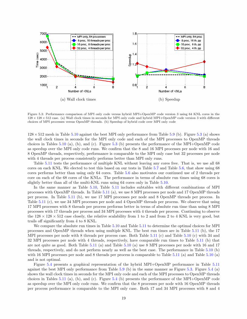
Figure 5.3: Performance comparison of MPI only code versus hybrid MPI+OpenMP code version 3 using 64 KNL cores in the128× 128× 512 case. (a) Wall clock times in seconds for MPI only code and hybrid MPI+OpenMP code version 3 with differentchoices of MPI processes versus OpenMP threads. (b) Speedup of hybrid code over MPI only code

128× 512 mesh in Table 5.10 against the best MPI only performance from Table 5.9 (b). Figure 5.3 (a) showsthe wall clock times in seconds for the MPI only code and each of the MPI processes to OpenMP threadschoices in Tables 5.10 (a), (b), and (c). Figure 5.3 (b) presents the performance of the MPI+OpenMP codeas speedup over the MPI only code runs. We confirm that the 8 and 16 MPI processes per node with 16 and8 OpenMP threads, respectively, performance is comparable to the MPI only case but 32 processes per nodewith 4 threads per process consistently performs better than MPI only runs.

Table 5.11 tests the performance of multiple KNL without leaving any cores free. That is, we use all 68cores on each KNL. We elected to test this based on our tests in Table 5.7 and Table 5.6, that show using 68cores performs better than using only 64 cores. Table 5.6 also motivates our continued use of 2 threads percore on each of the 68 cores of the KNLs. The performance in terms of absolute run times using 68 cores isslightly better than all of the multi-KNL runs using 64 cores only in Table 5.10.

In the same manner as Table 5.10, Table 5.11 includes subtables with different combinations of MPIprocesses with OpenMP threads. In Table 5.11 (a), we use 8 MPI processes per node and 17 OpenMP threadsper process. In Table 5.11 (b), we use 17 MPI processes per node and 8 OpenMP threads per process. InTable 5.11 (c), we use 34 MPI processes per node and 4 OpenMP threads per process. We observe that using17 MPI processes with 8 threads per process performs better in terms of absolute run time than using 8 MPIprocesses with 17 threads per process and 34 MPI processes with 4 threads per process. Continuing to observethe 128 × 128 × 512 case closely, the relative scalability from 1 to 2 and from 2 to 4 KNL is very good, buttrails off significantly from 4 to 8 KNL.

We compare the absolute run times in Table 5.10 and Table 5.11 to determine the optimal choices for MPIprocesses and OpenMP threads when using multiple KNL. The best run times are in Table 5.11 (b), the 17MPI processes per node with 8 threads per process case. Both Table 5.11 (c) and Table 5.10 (c) with 34 and32 MPI processes per node with 4 threads, respectively, have comparable run times to Table 5.11 (b) thatare not quite as good. Both Table 5.11 (a) and Table 5.10 (a) use 8 MPI processes per node with 16 and 17threads, respectively, and do not perform nearly as well as the best case. The performance in Table 5.10 (b)with 16 MPI processes per node and 8 threads per process is comparable to Table 5.11 (a) and Table 5.10 (a)and is not optimal.

Figure 5.4 presents a graphical representation of the hybrid MPI+OpenMP performance in Table 5.11against the best MPI only performance from Table 5.9 (b) in the same manner as Figure 5.3. Figure 5.4 (a)shows the wall clock times in seconds for the MPI only code and each of the MPI processes to OpenMP threadschoices in Tables 5.11 (a), (b), and (c). Figure 5.4 (b) presents the performance of the MPI+OpenMP codeas speedup over the MPI only code runs. We confirm that the 8 processes per node with 16 OpenMP threadsper process performance is comparable to the MPI only case. Both 17 and 34 MPI processes with 8 and 4

19

Table 5.11: CICR strong scalability study of multiple KNL nodes with hybrid MPI+OpenMP code version 3. Observed wallclock times in units of HH:MM:SS on multiple KNL nodes in Flat Quadrant Configuration. For each KNL 68 cores are used with2 threads per core for a total of 136 threads and KMP AFFINITY=scatter in all cases.

MPI+OpenMP – Flat Quadrant, MCDRAM only(2 threads per core, 68 cores)

(a) 8 processes per node, 17 threads per processNumber of KNLs 1 2 4 8

16× 16× 64 00:00:08 00:00:08 00:00:07 (**)32× 32× 128 00:00:35 00:00:34 00:00:32 00:00:2664× 64× 256 00:08:00 00:04:21 00:04:00 00:04:13

128× 128× 512 01:54:32 00:58:48 00:30:49 00:28:18

(b) 17 processes per node, 8 threads per processNumber of KNLs 1 2 4 8

16× 16× 64 00:00:09 (**) (**) (**)32× 32× 128 00:00:31 00:00:30 (**) (**)64× 64× 256 00:06:07 00:03:25 00:03:55 (**)

128× 128× 512 01:25:39 00:45:40 00:23:49 00:21:42

(c) 34 processes per node, 4 threads per processNumber of KNLs 1 2 4 8

16× 16× 64 (**) (**) (**) (**)32× 32× 128 00:00:40 (**) (**) (**)64× 64× 256 00:06:28 00:04:14 (**) (**)

128× 128× 512 01:27:04 00:48:01 00:27:48 (**)

(a) Wall clock times (b) Speedup

Figure 5.4: Performance comparison of MPI only code versus hybrid MPI+OpenMP code version 3 using 68 KNL cores in the128× 128× 512 case. (a) Wall clock times in seconds for MPI only code and hybrid MPI+OpenMP code version 3 with differentchoices of MPI processes versus OpenMP threads. (b) Speedup of hybrid code over MPI only code

threads per processes, respectively, perform better than the MPI only case.We can also compare Figures 5.3 and 5.4 to observe the speedup increase using 68 cores rather than 64

cores. The best speedup over the best MPI only run in Figure 5.3 (b) is just over 1.2, but in Figure 5.4 (b) weobserve that both the 17 MPI processes with 8 OpenMP threads per process case and the 34 processes with4 threads per process case have better than 1.2 speedup for all cases. We confirm that the best performanceresults from 17 processes with 8 threads per process.

20

6. CONCLUSIONS AND OUTLOOK

We have demonstrated the potential for performance of complex codes on one as well as multiple KNLs usingadvantageous choices of the configurations modes based on the applications size and code characteristics. Weused the CICR problem from [2] to show performance for a specific complex application code. We discussedthe addition of OpenMP parallelism to an existing MPI code and presented two different implementationswith performance differences. This showed the need for hybrid MPI+OpenMP code implemented well for bestperformance. We also demonstrated the feasibility and benefit to using multiple KNL nodes.

The CICR code requires more demanding and significant communication and is more computationallyintensive than the Poisson problem from [7, 18]. This application code put additional burden on the MPI com-munication and the balance with OpenMP threads. We observed this effect with two different MPI+OpenMPimplementations. Careful memory observations showed the difference in memory overhead for MPI processesversus OpenMP threads as a benefit to OpenMP multi-threading parallelism. Memory observations confirmedthat the careful memory management of this special purpose code enables us to study very fine meshes forphysiological studies, like 128× 128× 512, in the 16 GB of MCDRAM on the KNL. We tested the scalabilityof the MPI only code and the OpenMP scalability with hybrid MPI+OpenMP code on a single KNL andconfirmed the benefit of using multiple KNL nodes.

With two different hybrid MPI+OpenMP code implementations, we considered the number and placementof OpenMP threads relative to the number of MPI processes used and assessed the optimal number of OpenMPthreads per core on the KNL. The different implementations show different balances in performance withOpenMP threads versus MPI processes. The intermediate version 2 of the code clearly does not performbetter than the original MPI-only version, which demonstrates that diligent work might be needed, such as inprogramming OpenMP pragmas in all needed places. We demonstrate here that the x86 compatibility of eachPhi core is an advantage here, since it is possible to make incremental progress and to analyze performance,e.g., with VTune or other analyzing tools, at each step. Our final OpenMP implementation that implementedmulti-threading also in the function with the non-linear reaction coupling terms demonstrated significantlybetter performance with fewer MPI processes and more multi-threading. We observed that optimal choicesfor OpenMP threads to MPI processes and threads per core depended on the mesh resolution of the problem.For coarser meshes, more OpenMP threads to MPI processes performed better, but for finer meshes, usingmore MPI processes relative to the number of threads performed better. Since in reality, simulations usingdifferent mesh resolutions are often desired, e.g., a coarser one for large numbers of simulations for parameterstudies or in uncertainty quantification vs. a finer mesh to produce high-resolution images, the flexibility ofhaving a hybrid MPI+OpenMP code is useful.

We demonstrated scalability using multiple KNL with MPI only and our hybrid MPI+OpenMP code andobserved the need to choose the optimal number and combination of MPI processes and OpenMP threadsfor best performance. The code scales well for the finest meshes for small numbers of KNLs and when usinga small number of threads or cores. As observed on a single KNL, the best combinations of MPI processesand OpenMP threads using hybrid code on multiple KNLs outperformed using either MPI or OpenMP only,demonstrating the need for both in efficient production code. We observed that some choices of the distributionof MPI process to OpenMP threads result in poor performance relative to the best cases. In summary, formulti-KNL runs for our sample code, it is shown to be optimal to use all cores of each KNL, one MPI processon every other tile, and only two of the maximum of four threads per core. That is, the optimal combinationof MPI processes and OpenMP threads per process uses a total of 17 MPI processes per node and 8 OpenMPthreads per process. These specific results apply to this particular code, so researchers will have to experimentwith their code. The result that it is benficial to use all cores, without leaving any idling, indicates to alsoinvestigate this possibility.

This work enables further study of the KNL performance using the full 8 species of the CICR modelcoupling both the mechanical contraction and electrical excitation systems to the calcium signaling system.With a firm understanding of KNL performance with the code, we can make use of 2 and 4 KNL nodes to runsimulations efficiently to final times of 1,000 ms or more, rather than the 10 ms in the performance studiescontained here. This is necessary for upcoming parameter studies of the additional components of the modeland also since, for instance, laboratory time scales for this problem are on the order of minutes or only a modestmultiple longer than achieved by 1,000 ms. We can explicitly test performance with different vectorizationlevels using the options of the Intel compiler and will continue to optimize OpenMP implementation choices.

21

Additionally, we have the opportunity to continue to improve the numerical methods in the code to takeadvantage of the features of the KNL.

ACKNOWLEDGMENTS

This work used the Extreme Science and Engineering Discovery Environment (XSEDE), which is supported byNational Science Foundation grant number ACI–1053575 [25]. We acknowledge the Texas Advanced Comput-ing Center (TACC) at The University of Texas at Austin for providing HPC resources that have contributedto the research results reported within this paper. We also acknowledge the UMBC High Performance Com-puting Facility (HPCF). The facility is supported by the U.S. National Science Foundation through the MRIprogram (grant nos. CNS–0821258 and CNS–1228778) and the SCREMS program (grant no. DMS–0821311),with additional substantial support from the University of Maryland, Baltimore County (UMBC). JonathanGraf was supported by UMBC as HPCF RA.

REFERENCES

[1] Alexander, A. M., DeNardo, E. K., Frazier III, E., McCauley, M., Rojina, N., Coulibaly, Z., Peercy,B. E., Izu”, L. T., 2015. ”spontaneous calcium release in cardiac myocytes: Store overload and electricaldynamics”. Spora: A Journal of Biomathematics 1, 36–48.URL http://ir.library.illinoisstate.edu/spora/vol1/iss1/6

[2] Angeloff, K., Barajas, C. A., Middleton, A., Osia, U., Graf, J. S., Gobbert, M. K., Coulibaly, Z., 2016.Examining the effect of introducing a link from electrical excitation to calcium dynamics in a cardiomy-ocyte. Spora: A Journal of Biomathematics 2, 49–73.URL http://ir.library.illinoisstate.edu/spora/vol2/iss1/6

[3] Brewster, M. W., Graf, J. S., Huang, X., Coulibaly, Z., Gobbert, M. K., Peercy, B. E., 2015. Calciuminduced calcium release with stochastic uniform flux density in a heart cell. In: Mittal, S., Moon, I.-C.,Syriani, E. (Eds.), Proceedings of the Conference on Summer Computer Simulation. SummerSim ’15.Society for Computer Simulation International, pp. 1–6.

[4] Centers for Disease Control and Prevention, National Center for Health Statistics, 2015. Number ofdeaths for leading causes. https://www.cdc.gov/nchs/fastats/leading-causes-of-death.htm, pagelast reviewed March 17, 2017; accessed January 08, 2018.

[5] Gaeta, S. A., Krogh-Madsen, T., Christini, D. J., 2010. Feedback-control induced pattern formation incardiac myocytes: a mathematical modeling study. J. Theor. Biol. 266 (3), 408–418.

[6] Gobbert, M. K., 2008. Long-time simulations on high resolution meshes to model calcium waves in aheart cell. SIAM J. Sci. Comput. 30 (6), 2922–2947.

[7] Graf, J. S., 2017. Parallel Performance of Numerical Simulations for Applied Partial Differential EquationModels on the Intel Xeon Phi Knights Landing Processor. Ph.D. Thesis, Department of Mathematics andStatistics, University of Maryland, Baltimore County.

[8] Hanhart, A. L., Gobbert, M. K., Izu, L. T., 2004. A memory-efficient finite element method for systemsof reaction-diffusion equations with non-smooth forcing. J. Comput. Appl. Math. 169 (2), 431–458.

[9] Huang, X., 2015. An MPI-CUDA Implementation of a Model for Calcium Induced Calcium Release in aThree-Dimensional Heart Cell on a Hybrid CPU/GPU Cluster. Ph.D. Thesis, Department of Mathematicsand Statistics, University of Maryland, Baltimore County.

[10] Huang, X., Gobbert, M. K., 2015. Parallel performance studies for a three-species application problem onthe cluster maya. Tech. Rep. HPCF–2015–8, UMBC High Performance Computing Facility, University ofMaryland, Baltimore County.URL www.umbc.edu/hpcf

22

http://ir.library.illinoisstate.edu/spora/vol1/iss1/6

http://ir.library.illinoisstate.edu/spora/vol2/iss1/6

https://www.cdc.gov/nchs/fastats/leading-causes-of-death.htm

www.umbc.edu/hpcf

[11] Intel, June 23 2014. Intel re-architects the fundamental building block for high-performance computing — Intel newsroom. https://newsroom.intel.com/news-releases/

intel-re-architects-the-fundamental-building-block-for-high-performance-computing/,accessed January 08, 2018.

[12] Intel, 2015. Thread affinity interface. https://software.intel.com/en-us/node/522691#AFFINITY_

TYPES, accessed January 08, 2018.

[13] Intel, 2016. Controlling thread allocation. https://software.intel.com/en-us/node/694293, accessedJanuary 08, 2018.

[14] Intel, 2016. Intel Xeon Phi processor 7250 (16 GB, 1.40 GHz, 68 core) specifications. http:

//ark.intel.com/products/94035/Intel-Xeon-Phi-Processor-7250-16GB-1_40-GHz-68-core, ac-cessed January 08, 2018.

[15] Intel, 2016. MCDRAM (high bandwidth memory) on Knights Landing —analysis methods & tools. https://software.intel.com/en-us/articles/

mcdram-high-bandwidth-memory-on-knights-landing-analysis-methods-tools, accessed Jan-uary 08, 2018.

[16] Intel, 2016. Process and thread affinity for Intel Xeon Phi processors. https://software.intel.com/en-us/articles/process-and-thread-affinity-for-intel-xeon-phi-processors-x200, accessedJanuary 08, 2018.

[17] Izu, L. T., Means, S. A., Shadid, J. N., Chen-Izu, Y., Balke, C. W., 2006. Interplay of ryanodine receptordistribution and calcium dynamics. Biophys. J. 91, 95–112.

[18] Jabbie, I. A., Owen, G., Whiteley, B., 2017. Performance comparison of Intel Xeon Phi Knights Landing.SIAM Undergraduate Research Online (SIURO) 10.

[19] KNL User Guide, 2016. Stampede KNL cluster user guide. https://portal.tacc.utexas.edu/

user-guides/stampede#stampede-knl-clusterknl.

[20] Qu, Z., Nivala, M., Weiss, J. N., 2013. Calcium alternans in cardiac myocytes: Order from disorder. J.Mol. Cell. Cardiol. 58, 100–109.

[21] Rosales, C., James, D., Gomez-Iglesias, A., Cazes, J., Huang, L., Liu, H., Liu, S., Barth, W., 2016. KNLutilization guidelines. Tech. Rep. TR–16–03, Texas Advanced Computing Center, The University of Texasat Austin.

[22] Schafer, J., Huang, X., Kopecz, S., Birken, P., Gobbert, M. K., Meister, A., 2015. A memory-efficientfinite volume method for advection-diffusion-reaction systems with non-smooth sources. Numer. MethodsPartial Differential Equations 31 (1), 143–167.

[23] Sodani, A., 2015. Intel Xeon Phi processor “Knights Landing” architectural overview. https://www.

nersc.gov/assets/Uploads/KNL-ISC-2015-Workshop-Keynote.pdf, accessed January 08, 2018.

[24] Sodani, A., Gramunt, R., Corbal, J., Kim, H. S., Vinod, K., Chinthamani, S., Hutsell, S., Agarwal, R.,Liu, Y. C., 2016. Knights Landing: Second-generation Intel Xeon Phi product. IEEE Micro 32 (2), 34–46.

[25] Towns, J., Cockerill, T., Dahan, M., Foster, I., Gaither, K., Grimshaw, A., Hazlewood, V., Lathrop,S., Lifka, D., Peterson, G. D., Roskies, R., Scott, J. R., Wilkins-Diehr, N., 2014. XSEDE: Acceleratingscientific discovery. Comput. Sci. Eng. 16 (5), 62–74.

23

https://newsroom.intel.com/news-releases/intel-re-architects-the-fundamental-building-block-for-high-performance-computing/

https://newsroom.intel.com/news-releases/intel-re-architects-the-fundamental-building-block-for-high-performance-computing/

https://software.intel.com/en-us/node/522691#AFFINITY_TYPES

https://software.intel.com/en-us/node/522691#AFFINITY_TYPES

https://software.intel.com/en-us/node/694293

http://ark.intel.com/products/94035/Intel-Xeon-Phi-Processor-7250-16GB-1_40-GHz-68-core

http://ark.intel.com/products/94035/Intel-Xeon-Phi-Processor-7250-16GB-1_40-GHz-68-core

https://software.intel.com/en-us/articles/mcdram-high-bandwidth-memory-on-knights-landing-analysis-methods-tools

https://software.intel.com/en-us/articles/mcdram-high-bandwidth-memory-on-knights-landing-analysis-methods-tools

https://software.intel.com/en-us/articles/process-and-thread-affinity-for-intel-xeon-phi-processors-x200

https://software.intel.com/en-us/articles/process-and-thread-affinity-for-intel-xeon-phi-processors-x200

https://portal.tacc.utexas.edu/user-guides/stampede#stampede-knl-clusterknl

https://portal.tacc.utexas.edu/user-guides/stampede#stampede-knl-clusterknl

https://www.nersc.gov/assets/Uploads/KNL-ISC-2015-Workshop-Keynote.pdf

https://www.nersc.gov/assets/Uploads/KNL-ISC-2015-Workshop-Keynote.pdf

Long-time Simulations with Complex Code Using Multiple ...gobbert/papers/Graf_JCAM2017.pdfLong-time...

Documents

Transcript of Long-time Simulations with Complex Code Using Multiple ...gobbert/papers/Graf_JCAM2017.pdfLong-time...