Long-Term Satellite Record RevealsLikely Recent Aerosol TrendMichael I. Mishchenko,* Igor V. Geogdzhayev, William B. Rossow, Brian Cairns,Barbara E. Carlson, Andrew A. Lacis, Li Liu, Larry D. Travis

Recent observations of downward solarradiation fluxes at Earth’s surface haveshown a recovery from the previous de-

cline known as global “dimming” (1), with the“brightening” beginning around 1990 (2). The in-creasing amount of sunlight at the surface pro-foundly affects climate and may represent certaindiminished counterbalances to greenhouse gaswarming, thereby making the warming trendmore evident during the past decade.

It has been suggested that tropospheric aero-sols have contributed notably to the switch fromsolar dimming to brightening via both directand indirect aerosol effects (1, 2). It has furtherbeen argued (3) that the solar radiation trendmirrors the estimated recent trend in primary an-thropogenic emissions of SO2 and black carbon,which contribute substantially to the global aero-sol optical thickness (AOT). A similar increaseof net solar flux at the top of the atmosphere(TOA) over the same period appears to beexplained by corresponding changes in lower-latitude cloudiness (4), which confounds theinterpretation of the surface radiation record.Therefore, it is important to provide a direct andindependent assessment of the actual global long-term behavior of the AOT. We accomplish thisby using the longest uninterrupted record ofglobal satellite estimates of the column AOTover the oceans, the Global Aerosol ClimatologyProject (GACP) record (5). The record is derivedfrom the International Satellite Cloud ClimatologyProject (ISCCP) DX radiance data set composedof calibrated and sampled Advanced Very HighResolution Radiometer (AVHRR) radiances. Adetailed discussion of the sampling resolution,calibration history, and changes in the corre-sponding satellite sensors can be found in (6).

The global monthly average of the columnAOT is depicted for the period August 1981 toJune 2005 (Fig. 1, solid black curve). The twomajor maxima are caused by the stratosphericaerosols generated by the El Chichon (March1982) and the Mount Pinatubo (June 1991) erup-tions, also captured in the Stratospheric Aerosoland Gas Experiment (SAGE) stratospheric AOTrecord (7). The quasi-periodic oscillations in theblack curve are the result of short-term aerosolvariability.

The overall behavior of the column AOTduring the eruption-free period from January 1986to June 1991 (Fig. 1, red line) shows only a hintof a statistically significant tendency and indicatesthat the average column AOT value just beforethe Mount Pinatubo eruption was close to 0.142.After the eruption, the GACP curve is a super-position of the complex volcanic and troposphericAOT temporal variations. However, the green linereveals a long-term decreasing tendency in thetropospheric AOT. Indeed, even if we assume thatthe stratospheric AOT just before the eruptionwas as large as 0.007 and that by June 2005 thestratospheric AOT became essentially zero (com-pare with the blue curve), still the resulting de-crease in the tropospheric AOT during the 14-yearperiod comes out to be 0.03. This trend issignificant at the 99% confidence level.

Admittedly, AVHRR is not an instrument de-signed for accurate aerosol retrievals from space.Among the remaining uncertainties is radiancecalibration, which, if inaccurate, can result inspurious aerosol tendencies. Similarly, substan-tial systematic changes in the aerosol single-scattering albedo or the ocean reflectance can bemisinterpreted in terms of AOT variations. How-ever, the successful validation of GACP retriev-

als using precise sun photometer data takenfrom 1983 through 2004 (8, 9) indicates that theISCCP radiance calibration is likely to be re-liable. This conclusion is reinforced by the closecorrespondence of calculated and observed TOAsolar fluxes (4). Furthermore, the GACP AOTrecord appears to be self-consistent, with nodrastic intrasatellite variations, and is consistentwith the SAGE record.

The advantage of the AVHRR data set overthe data sets collected with more advanced re-cent satellite instruments is its duration, whichmakes possible reliable detection of statisticallysignificant tendencies like the substantial de-crease of the tropospheric AOT between 1991and 2005. With all the uncertainties, the tropo-spheric AOT decrease over the 14-year period isestimated to be at least 0.02. This change is con-sistent with long-term atmospheric transmissionrecords collected in the former Soviet Union (5).

Our results suggest that the recent downwardtrend in the tropospheric AOT may have contrib-uted to the concurrent upward trend in surfacesolar fluxes. Neither AVHRR nor other existingsatellite instruments can be used to determineunequivocally whether the recent AOT trend isdue to long-term global changes in natural or an-thropogenic aerosols. This discrimination wouldbe facilitated by an instrument like the AerosolPolarimetry Sensor (APS), scheduled for launchin December 2008 as part of the NASA Glorymission (10). It is thus imperative to provide un-interrupted multidecadal monitoring of aerosolsfrom space with dedicated instruments like APSin order to detect long-term anthropogenic trendspotentially having a strong impact on climate.

References and Notes1. M. Wild et al., Science 308, 847 (2005).2. R. T. Pinker, B. Zhang, E. G. Dutton, Science 308, 850

(2005).3. D. G. Streets, Y. Wu, M. Chin, Geophys. Res. Lett. 33,

L15806 (2006).4. Y. Zhang, W. B. Rossow, A. A. Lacis, V. Oinas,

M. I. Mishchenko, J. Geophys. Res. 109, D19105 (2004).5. I. V. Geogdzhayev, M. I. Mishchenko, E. I. Terez,

G. A. Terez, G. K. Gushchin, J. Geophys. Res. 110,D23205 (2005); and references therein.

6. W. B. Rossow, R. A. Schiffer, Bull. Am. Meteorol. Soc. 80,2261 (1999); and references therein.

7. J. Hansen et al., J. Geophys. Res. 107, 4347 (2002).8. L. Liu et al., J. Quant. Spectrosc. Radiat. Transfer 88, 97

(2004).9. A. Smirnov et al., Geophys. Res. Lett. 33, L14817

(2006).10. M. I. Mishchenko et al., J. Quant. Spectrosc. Radiat.

Transfer 88, 149 (2004).11. This research is part of NASA/Global Energy and Water

Cycle Experiment GACP and was funded by the NASARadiation Sciences Program, managed by H. Maring andD. Anderson.

24 October 2006; accepted 20 December 200610.1126/science.1136709

BREVIA

NASA Goddard Institute for Space Studies, 2880 Broadway,New York, NY 10025, USA.

*To whom correspondence should be addressed. E-mail:mmishchenko@giss.nasa.gov

Year

0

0.1

0.2

0.3

0.4

Opt

ical

thic

knes

s

81 82 83 84 85 86 87 88 89 90 91 92 93 94 95 96 97 98 99 00 01 02 03 04 05

GACPSAGE

Pinatubo

El Chichon

Fig. 1. GACP record of the globally averaged column AOT over the oceans and SAGE record of theglobally averaged stratospheric AOT.

www.sciencemag.org SCIENCE VOL 315 16 MARCH 2007 1543

on

Mar

ch 2

4, 2

007

ww

w.s

cien

cem

ag.o

rgD

ownl

oade

d fr

om

REVIEW

Perspectives on the Arctic’sShrinking Sea-Ice CoverMark C. Serreze,1* Marika M. Holland,2 Julienne Stroeve1

Linear trends in arctic sea-ice extent over the period 1979 to 2006 are negative in every month. This iceloss is best viewed as a combination of strong natural variability in the coupled ice-ocean-atmospheresystem and a growing radiative forcing associated with rising concentrations of atmospheric greenhousegases, the latter supported by evidence of qualitative consistency between observed trends and thosesimulated by climate models over the same period. Although the large scatter between individual modelsimulations leads to much uncertainty as to when a seasonally ice-free Arctic Ocean might be realized, thistransition to a new arctic state may be rapid once the ice thins to a more vulnerable state. Loss of the icecover is expected to affect the Arctic’s freshwater system and surface energy budget and could bemanifested in middle latitudes as altered patterns of atmospheric circulation and precipitation.

Themost defining feature of theArcticOceanis its floating sea-ice cover, which hastraditionally ranged fromamaximumextent

of about 16 × 106 km2 in March to a minimumextent of 7 × 106 km2 at the end ofthe summer melt season in Sep-tember (Fig. 1). Consistent satellite-derived monthly time series ofsea-ice extent are provided by theNimbus-7 Scanning MultichannelMicrowave Radiometer (October1978 to August 1987) and theDefense Meteorological SatelliteProgram Special Sensor Microwave/Imager (1987 to present). Based onregression analysis of the combinedrecord over the period 1979 to 2006,ice extent has declined for everymonth (Fig. 2), most rapidly forSeptember, for which the trend is–8.6 ± 2.9% per decade or about100,000 km2 per year. Ice extent isdefined as the area of the oceanwitha fractional ice cover (i.e., an iceconcentration) of at least 15% (1–3).

Every year since 2001 hasyielded pronounced Septemberminima, the most extreme of whichwas in 2005 (5.56 ×106 km2).Whencompared to the mean ice extentover the period 1979 to 2000, thisrepresents a spatial reduction of21% (1.6 × 106 km2), an area roughly the sizeof Alaska (Fig. 1). Comparisons with earlierrecords, which combine visible-band satellite im-agery and aircraft and ship reports, suggest that

the September 2005 ice extent was the lowest inat least the past 50 years. Data for the past fewyears suggest an accelerating decline in wintersea-ice extent (4).

Evidence for accompanying reductions in icethickness (5) is inconclusive. Upward-lookingsonar aboard submarines provides informationon ice draft—the component of the total thick-ness (about 90%) that projects below the watersurface. Comparisons between early sonar records(1958 to 1976) and those for 1993 to 1997 indicatereductions of 1.3 m inmean late summer ice draftover much of the central Arctic Ocean (6), butsparse sampling complicates interpretation. Fur-ther analysis of the submarine-acquired data in

conjunction with model simulations points tothinning through 1996 but modest recoverythereafter (7). Results from an ice-tracking al-gorithm applied to satellite data from 1978 to2003 document decreasing coverage of old, thickice (8).

Understanding the Observed Ice LossThe observed decline in ice extent reflects a con-flation of thermodynamic and dynamic processes.Thermodynamic processes involve changes insurface air temperature (SAT), radiative fluxes,and ocean conditions. Dynamic processes involvechanges in ice circulation in response to windsand ocean currents. These include changes in thestrength and location of the Beaufort Gyre (amean annual clockwise motion in the westernArctic Ocean) and characteristics of the Trans-polar Drift Stream (a motion of ice that progressesfrom the coast of Siberia, across the pole, and intothe North Atlantic via the Fram Strait). Nearly allof the ice export from the Arctic to the Atlanticoccurs through this narrow strait betweennorthern Greenland and Svalbard (Fig. 1).

Estimated rates of SAT changeover the Arctic Ocean for the pastseveral decades vary depending onthe time period and season, as wellas the data source being consid-ered. Although natural variabilityplays a large role in SAT variations,the overall pattern is one of recentwarming, which is in turn part of aglobal signal (9). Using a record thatcombined coastal station obser-vationswithdata fromdriftingbuoys(from 1979 onward) and Russian“North Pole” stations (1950 to1991), Rigor et al. (10) foundpositive SAT trends from 1979 to1997 that were most pronouncedand widespread during spring. Al-though there are biases in the buoydata relative to the North Pole data,especially for October throughApril (11), independent evidencefor warming during spring, sum-mer, and autumn since 1981 isdocumented in clear-sky surfacetemperatures retrieved from ad-vanced very-high-resolution radio-meter satellite imagery (12).

Further support for warming comes from analysisof satellite-derived passive microwave brightnesstemperatures that indicate earlier onset of springmelt and lengthening of the melt season (13), aswell as from data from the Television InfraredObservation Satellites Operational Vertical Soun-der that point to increased downwelling radiationto the surface in spring over the past decade,which is linked to increased cloud cover andwater vapor (14). Our assessments of autumn andwinter data fields from the National Centers for

1Cooperative Institute for Research in EnvironmentalSciences, National Snow and Ice Data Center, CampusBox 449, University of Colorado, Boulder, CO 80309–0449, USA. 2National Center for Atmospheric Research,Post Office Box 3000, Boulder, CO 80307, USA.

*To whom correspondence should be addressed. E-mail:serreze@kryos.colorado.edu

Fig. 1. Sea-ice extent (bright white area) for September 2005. Median iceextents based on the period 1979 to 2000 for September (red line) andMarch (blue line) illustrate the typical seasonal range. Geographic featuresreferred to in the text are labeled. Credit: NSIDC image in Google Earth.

www.sciencemag.org SCIENCE VOL 315 16 MARCH 2007 1533

SPECIALSECTION

on

Mar

ch 2

4, 2

007

ww

w.s

cien

cem

ag.o

rgD

ownl

oade

d fr

om

Environmental Prediction and National Center forAtmospheric Research (NCEP-NCAR) reanalysis(15) point to strong surface and low-level warm-ing for the period 2000 to 2006 relative to 1979 to1999. Weaker warming is evident for summer.

All of these results are consistent with a declin-ing ice cover. However, at least part of the recentcold-season warming seen in the NCEP-NCARdata is itself driven by the loss of ice, because thisloss allows for stronger heat fluxes from the ocean tothe atmosphere. The warmer atmosphere will thenpromote a stronger longwave flux to the surface.

Links have also been established between iceloss and changes in ice circulation associated withthe behavior of the North Atlantic Oscillation(NAO),NorthernAnnularMode (NAM), and otheratmospheric patterns. The NAO refers to covari-ability between the strength of the Icelandic Lowand that of the Azores High, which are the twocenters of action in the North Atlantic atmosphericcirculation. When both are strong (or weak), theNAO is in its positive (or negative) phase. TheNAM refers to an oscillation of atmospheric massbetween the Arctic and middle latitudes and ispositive when arctic pressures are low and mid-latitude pressures are high. TheNAOandNAMare

closely related and can be largely viewed as ex-pressions of the same phenomenon.

From about 1970 through the mid-1990s,winter indices of the NAO-NAM shifted fromnegative to strongly positive. Rigor et al. (16)showed that altered surface winds resulted in amore cyclonic motion of ice and an enhancedtransport of ice away from the Siberian andAlaskancoasts (i.e., a more pronounced Transpolar DriftStream). This change in circulation fostered open-ings in the ice cover. Although these openingsquickly refroze in response to low winter SATs,coastal areas in springwere nevertheless left with ananomalous coverage of young, thin ice. This thin icethenmelted out in summer, whichwas expressed aslarge reductions in ice extent. Summer ice loss wasfurther enhanced as the thinner ice promotedstronger heat fluxes to the atmosphere, fosteringhigher spring air temperatures and earliermelt onset.

Given that the NAO-NAM has regressed backto a more neutral state since the late 1990s (17),these processes cannot readily explain the extremeSeptember sea-ice minima of recent years. Rigorand Wallace (18) argued that recent extremesrepresent delayed impacts of the very stronglypositive winter NAO-NAM state from about 1989

to 1995. As the NAO-NAM rose to this positivestate, shifts in the wind field not only promoted theproduction of thinner spring ice in coastal areas butflushed much of the Arctic’s store of thick ice intothe North Atlantic through Fram Strait.

Rothrock and Zhang (19) modified this view.Using a coupled ice-ocean model, they arguedthat although wind forcing was the dominantdriver of declining ice thickness and volumefrom the late 1980s through mid-1990s, the iceresponse to generally rising air temperatures wasmore steadily downward over the study period(1948 to 1999). In other words, without theNAO-NAM forcing, there would still have beena downward trend in ice extent, albeit smallerthan that observed. Lindsay and Zhang (20) cameto similar conclusions in their modeling study.Rising air temperature has reduced ice thickness,but changes in circulation also flushed some ofthe thicker ice out of the Arctic, leading to moreopen water in summer and stronger absorption ofsolar radiation in the upper (shallower depths ofthe) ocean. With more heat in the ocean, thinnerice grows in autumn and winter.

Recent years have experienced patterns ofatmospheric circulation in spring and summer fa-

January

July September

Ice

Ext

ent (

mill

ion

squa

re k

m)

Ice

Ext

ent (

mill

ion

squa

re k

m)

Ice

Ext

ent (

mill

ion

squa

re k

m)

Ice

Ext

ent (

mill

ion

squa

re k

m)

Ice

Ext

ent (

mill

ion

squa

re k

m)

Ice

Ext

ent (

mill

ion

squa

re k

m)

November

March May

YearYear

Year Year Year

Year

18 19 16

15

14

13

12

11

18

17

16

15

14

13

17

16

15

14

13

13 14

13

12

11

10

9

8

12

11

10

9

9

8

7

6

5

8

7

121975 1980 1985 1990 1995 2000 2005 2010 1975 1980 1985 1990 1995 2000 2005 2010 1975 1980 1985 1990 1995 2000 2005 2010

1975 1980 1985 1990 1995 2000 2005 2010 1975 1980 1985 1990 1995 2000 2005 2010 1975 1980 1985 1990 1995 2000 2005 2010

–3.1 (+ / –0.8) % per decade

–5.5 (+ / –1.6) % per decade

–2.8 (+ / –0.8) % per decade

–8.6 (+ / –2.9) % per decade

–2.8 (+ / –1.1) % per decade

–4.4 (+ / –1.3) % per decade

Fig. 2. Time series of arctic sea-ice extent for alternate months and least-squares linear fit based on satellite-derived passive microwave data fromNovember 1979 through November 2006. Listed trends include (in

parentheses) the 95% confidence interval of the slope. Ice extent is alsodeclining for the six months that are not shown, ranging from –2.8 ± 0.8%per decade in February to –7.2 ± 2.3% per decade in August.

16 MARCH 2007 VOL 315 SCIENCE www.sciencemag.org1534

Polar Science

on

Mar

ch 2

4, 2

007

ww

w.s

cien

cem

ag.o

rgD

ownl

oade

d fr

om

voring ice loss. By altering both the Beaufort Gyreand Transpolar Drift Stream, these patterns havereduced how long ice is sequestered and aged in theArctic Ocean (21). The strength of a cyclonic at-mospheric regime that sets up over the centralArctic Ocean in summer is important. Along withpromoting offshore ice motion, the pronouncedcyclonic summer circulations of 2002 and 2003 fa-vored ice divergence, as is evident from the low iceconcentrations in satellite imagery. Ice divergencein summer spreads the existing ice over a largerarea, but enhanced absorption of solar energy in theareas of open water promotes stronger melt. Therewas also very little September ice in the GreenlandSea (off the east coast of Greenland) for thesesummers, which may also be linked to winds asso-ciated with this summer atmospheric pattern (22).

To further complicate the picture, it appearsthat changes in ocean heat transport have played arole. Warm Atlantic waters enter the Arctic Oceanthrough eastern Fram Strait and the Barents Seaand form an intermediate layer as they subductbelow colder, fresher (less dense) arctic surfacewaters. Hydrographic data show increased importof Atlantic-derived waters in the early to mid-1990s and warming of this inflow (23). This trendhas continued, characterized by pronounced pulsesof warm inflow. Strong ocean warming in theEurasian basin in 2004 can be traced to a pulseentering the Barents Sea in 1997 and 1998. Themost recent data show another warm anomalypoised to enter the Arctic Ocean (24, 25). Theseinflows may promote ice melt and discourage icegrowth along the Atlantic ice margin. Once At-lantic water enters the Arctic Ocean, the coldhalocline layer (CHL) separating the Atlantic andsurface waters largely insulates the ice from theheat of the Atlantic layer. Observations suggest aretreat of the CHL in the Eurasian basin in the1990s (26). This likely increasedAtlantic layer heat

loss and ice-ocean heat exchange. Partial recoveryof the CHL has been observed since 1998 (27).

Maslowski et al. (28) proposed a connectionbetween ice loss and oceanic heat flux through theBering Strait. However, hydrographic data col-lected between 1990 and 2004 document strongvariability in this inflow as opposed to a longer-term trend. An observed increase in the flux be-tween 2001 and 2004 is estimated to be capable ofmelting 640,000 km2 of 1-m-thick ice, but fluxes in2001 are the lowest of the record (29). Subsequentanalysis (30) nevertheless reveals a link between iceloss and increases in Pacific Surface Water (PSW)temperature in the Arctic Ocean beginning in thelate 1990s, concurrent with the onset of sharp sea-ice reductions in the Chukchi and Beaufort seas.The hypothesis that has emerged from those obser-vations is that delayed winter ice formation allowsfor more efficient coupling between the ocean andwind forcing. This redirects PSW from the shelfslope along Alaska into the Arctic Ocean, where itis more efficient in retarding winter ice growth. Animbalance between winter ice growth and summermelt results, accelerating ice loss over a large area.

To summarize, the observed sea-ice loss can inpart be connected to arctic warming over the pastseveral decades. Although this warming is part of aglobal signal suggesting a link with greenhouse gas(GHG) loading, attribution is complicated by a suiteof contributing atmospheric and oceanic forcings.Below we review the evidence for an impact ofGHG loading on the observed trends and projectionsfor the future, based on climate model simulations.

Simulations from Climate ModelsZhang and Walsh (31) showed that most of themodels used in the Intergovernmental Panel onClimate Change Fourth Assessment Report(IPCC AR4) have climatological sea-ice extentwithin 20%of the observed climatology over their

adopted base period of 1979 to 1999, with goodsimulation of the seasonal cycle. The multimodelensemble mean realistically estimates observedice extent changes over this base period, and mostindividual models also show a downward trend.Our analysis of an IPCC AR4 multimodel en-semble mean hindcast for the longer base period1979 to 2006 also reveals consistency with ob-servations regarding larger trends in Septemberversus those in winter. These results provide strongevidence that, despite prominent contributions ofnatural variability in the observed record, GHGloading has played a role.

Rates of ice loss both for the past few decadesand those projected through the 21st century never-theless vary widely between individual models.Our analyses show that in the IPCC AR4 modelsdriven with the Special Report on Emissions Sce-narios (SRES) A1B emissions scenario (in whichatmospheric CO2 reaches 720 parts per million by2100), a near-complete or complete loss (to lessthan 1 × 106 km2) of September ice will occuranywhere from2040 towell beyond the year 2100,depending on the model and the particular runfor that model. Overall, about half the modelsreach September ice-free conditions by 2100 (32).Figure 3 shows the spatial pattern of the percentof models that predict at least 15% fractionalice cover for March and September, averagingoutput over the period 2075–2084. Even by thelate 21st century, most models project a thin icecover in March. By contrast, about 40% of themodels project no ice in September over thecentral Arctic Ocean.

The scatter among models reflects many fac-tors, including the initial (late-20th century) sim-ulated ice state, aspects of the modeled oceancirculation, simulated cloud conditions, and naturalvariability in the modeled system (e.g., NAO-NAM–like behavior). These tie in strongly to thestrength and characteristics of thepositive ice-albedofeedback mechanism. In general, GHG loadingresults in a stronger and longer summermelt season,thinning the ice and exposingmore of the dark (lowalbedo) ocean surface that readily absorbs solar ra-diation. Autumn ice growth is delayed, resultingin thinner spring ice. This thin ice is more apt tomelt out during the next summer, exposing moreopenwater, which results in even thinner ice duringthe following spring. Negative feedbacks, such asthe fact that thinner ice grows more rapidly thanthicker ice when exposed to the same forcing, cancounteract these changes but are generally weaker.

Although there is ample uncertainty regardingwhen a seasonally ice-free Arctic Ocean will berealized, the more interesting question is how it ar-rives at that state. Simulations based on the Com-munity Climate SystemModel version 3 (CCSM3)(33) indicate that end-of-summer ice extent is sen-sitive to ice thickness in spring. If the ice thins to amore vulnerable state, a “kick” associated withnatural climate variability can result in rapid sum-mer ice loss because of the ice-albedo feedback. In

Fig. 3. Spatial pattern of the percent of IPCC AR4 model simulations (SRES A1B scenario) with at least15% ice concentration for March (left) and September (right), averaged over the decade 2075 to2084. For example, a value of 60% at a given locationmeans that 60% of simulations predicted sea ice.Results are based on 11 models with realistic 20th-century September sea-ice extent.

www.sciencemag.org SCIENCE VOL 315 16 MARCH 2007 1535

SPECIALSECTION

on

Mar

ch 2

4, 2

007

ww

w.s

cien

cem

ag.o

rgD

ownl

oade

d fr

om

the events simulated by CCSM3, anomalous oceanheat transport acts as this trigger. Such abrupt tran-sitions are typically four times as fast as the ob-served trends over the satellite record. In oneensemble member, September ice extent decreasesfrom about 6 × 106 to 2 × 106 km2 in 10 years,resulting in near ice-free September conditions by2040. A number of other climate models showsimilar rapid ice loss events.

ImpactsLoss of the sea-ice cover will have numerous im-pacts. A sharply warmer Arctic in autumn andwinter is expected as a result of larger heat fluxesfrom the ocean to the atmosphere. This is the pri-mary fingerprint of arctic amplification of green-house warming (34). As ice retreats from theshore, winds have a longer fetch over open water,resulting in more wave action. This effect is al-ready resulting in coastal erosion in Alaska andSiberia. Ice loss is also affecting traditional hunt-ing practices by members of indigenous culturesand contributing to regional declines in polar bearhealth and abundance (35).

In theirmodeling study,Magnusdottiret al. (36)found that declining ice in the Atlantic sector pro-motes a negative NAO-NAM atmospheric circu-lation response, with a weaker, southward-shiftedstorm track. Singarayer et al. (37) forced the HadleyCentre Atmospheric Model with observed sea icefrom 1980 to 2000 and projected sea-ice reductionsuntil 2100. In one simulation, mid-latitude stormtracks were intensified, increasing precipitation overwestern and southern Europe in winter. Experi-ments bySewall andSloan (38) revealed impacts onextrapolar precipitation patterns leading to reducedrainfall in the American West. Although resultsfrom different experiments with different designsvary, the common thread is that sea ice matters.

Climate models also indicate that by increasingupper-ocean stability and suppressing deepwaterformation, North Atlantic freshening may disruptthe global thermohaline circulation, possibly withfar-reaching consequences. Increased freshwaterexport from the Arctic is a potential source of suchfreshening. Observations implicate an arctic sourcefor freshening in the North Atlantic since the 1960s(39). Total freshwater output to theNorthAtlantic isprojected to increase through the 21st century, withdecreases in ice export more than compensatedby the liquid freshwater export. However, reduc-tions in ice melt and associated freshening in theGreenland-Iceland-Norwegian (GIN) seas resultingfrom a smaller ice transport through Fram Straitmay more directly affect the deepwater formationregions and counteract increased ocean stability dueto the warming climate (i.e., a warmer upper oceanis more stable). This outcome could help maintaindeepwater formation in the GIN seas (40).

ConclusionsNatural variability, such as that associated with theNAO-NAM and other circulation patterns, has and

will continue to have strong impacts on the arcticsea-ice cover. However, the observed ice loss forthe Arctic Ocean as a whole, including the largertrend for September as compared to that of winter,is qualitatively reproduced in ensemble meanclimate model hindcasts forced with the observedrise in GHG concentrations. This strongly suggestsa human influence (31). However, there is a largeamount of scatter between individual simulations,which contributes to uncertainty regarding rates ofice loss through the 21st century. An emerging is-sue is how a seasonally ice-free Arctic Ocean maybe realized: Will it result from a gradual declinewith strong imprints of natural variability, or couldthe transition be rapid once the ice thins to a morevulnerable state? Links between altered ocean heattransport and observed ice loss remain to be re-solved, as does the attribution of these transportchanges, but pulses such as those currently poisedto enter the Arctic Ocean from the Atlantic couldprovide a trigger for a rapid transition.

In this regard, future behavior of the CHL,which insulates the sea ice from the warm Atlanticlayer, is a key wild card. Another uncertainty is thebehavior of the NAO-NAM. Despite its return to amore neutral phase, there is evidence, albeit con-troversial, that external forcing may favor the pos-itive state that promotes ice loss. The mechanismsare varied but in part revolve around the idea thatstratospheric cooling in response to increasingGHG concentrations, or through ozone destruc-tion, may “spin up” the polar stratospheric vortex,resulting in lower arctic surface pressures. Anotherview is that the NAO-NAM could be bumped to apreferred positive state via warming of the tropicaloceans (41). However, as noted earlier, decliningsea ice in the Atlantic sector may invoke a negativeNAO-NAM response (36).

Given the agreement between models and ob-servations, a transition to a seasonally ice-freeArctic Ocean as the system warms seems in-creasingly certain. The unresolved questionsregard when this new arctic state will be realized,how rapid the transition will be, and what will bethe impacts of this new state on the Arctic and therest of the globe.

References and Notes1. Ice extent time series are available from the National

Snow and Ice Data Center (NSIDC) based on theapplication of the NASA team algorithm (used here) anda bootstrap algorithm to the passive microwavebrightness temperatures (http:/nsidc.org/data/seaice/).Trends computed from both are negative in all months,but those from the bootstrap series are slightly smaller(which yielded a September trend of –7.9% per decade).Trends are computed from anomalies referenced tomeans over the period 1979 to 2000. Surface melt insummer contaminates the passive microwave signal,resulting in the underestimation of ice concentration. Useof ice extent (a binary ice–no ice classification) largelycircumvents this problem.

2. Trends for all months are significant at the 99% confidencelevel, based on an F test with the null hypothesis of azero trend. Trends are also significant (exceeding the 95%level) based on the approach of Weatherhead et al. (3),

which computes the trend significance from the varianceand autocorrelation of the residuals.

3. E. C. Weatherhead et al., J. Geophys. Res. 103, 10.1029/98JD00995 (1998).

4. J. C. Comiso, Geophys. Res. Lett. 33, L18504 (2006).5. Ice thickness can be described from a probability

distribution, which has a peak at about 3 m. Although iceat the peak of the distribution is predominantly multiyearice that has survived one or more melt seasons andthicker than younger first-year ice (representing a singleyear’s growth), ridging can result in very thick first-yearice (up to 20 to 30 m).

6. D. A. Rothrock, Y. Yu, G. A. Maykut, Geophys. Res. Lett.26, 3469 (1999).

7. D. A. Rothrock, J. Zhang, Y. Yu, J. Geophys. Res. 108,3083 (2003).

8. C. Fowler, W. J. Emery, J. A. Maslanik, IEEE Geosci.Remote Sens. Lett. 1, 71 (2004).

9. M. C. Serreze, J. A. Francis, Clim. Change 76, 241 (2006).10. I. G. Rigor, R. L. Colony, S. Martin, J. Clim. 13, 896 (2000).11. I. V. Polyakov et al., J. Clim. 16, 2067 (2003).12. J. C. Comiso, J. Clim. 16, 3498 (2003).13. J. C. Stroeve, T. Markus, W. N. Meier, Ann. Glaciol. 25,

382 (2006).14. J. A. Francis, E. Hunter, EOS Trans. Am. Geophys. Union

87, 509 (2006).15. E. Kalnay et al., Bull. Am. Meteorol. Soc. 77, 437 (1996).16. I. G. Rigor, J. M. Wallace, R. L. Colony, J. Clim. 15, 2648

(2002).17. J. E. Overland, M. Wang, Geophys. Res. Lett. 32, L06701

(2005).18. I. G. Rigor, J. M. Wallace, Geophys. Res. Lett. 31, L09401

(2004).19. D. A. Rothrock, J. Zhang, J. Geophys. Res. 110, C01002

(2005).20. R. W. Lindsay, J. Zhang, J. Clim. 18, 4879 (2005).21. J. A. Maslanik, S. Drobot, C. Fowler, W. Emery, R. Barry,

Geophys. Res. Lett. 34, 10.1029/2006GL028269 (2007).22. J. C. Stroeve et al., Geophys. Res. Lett. 32, L04501 (2005).23. R. R. Dickson et al., J. Clim. 13, 2671 (2000).24. I. V. Polyakov et al., Geophys. Res. Lett. 32, L17605 (2005).25. W. Walczowski, J. Piechura, Geophys. Res. Lett. 33,

L12601 (2006).26. M. Steele, T. J. Boyd, J. Geophys. Res. 103, 10419 (1998).27. T. J. Boyd, M. Steele, R. D. Muench, J. T. Gunn, Geophys.

Res. Lett. 29, 1657 (2002).28. W. Maslowski, D. C. Marble, W. Walczowski, A. J. Semtner,

Ann. Glaciol. 33, 545 (2001).29. R. A. Woodgate, K. Aagaard, T. L. Weingartner, Geophys.

Res. Lett. 33, L15609 (2006).30. K. Shimada et al., Geophys. Res. Lett. 33, L08605 (2006).31. X. Zhang, J. E. Walsh, J. Clim. 19, 1730 (2006).32. O. Arzel, T. Fichefet, H. Goosse, Ocean Model. 12, 401

(2006).33. M. M. Holland, C. M. Bitz, B. Tremblay, Geophys. Res.

Lett. 33, L23503 (2006).34. S. Manabe, R. J. Stouffer, J. Geophys. Res. 85, 5529 (1980).35. I. Stirling, C. L. Parkinson, Arctic 59, 261 (2006).36. G. Magnusdottir, C. Deser, R. Saravanan, J. Clim. 17, 857

(2004).37. J. S. Singarayer, J. Bamber, P. J. Valdes, J. Clim. 19, 1109

(2006).38. J. O. Sewall, L. C. Sloan, Geophys. Res. Lett. 31, L06209

(2004).39. B. J. Peterson et al., Science 313, 1061 (2006).40. M. M. Holland, J. Finnis, M. C. Serreze, J. Clim. 19, 6221

(2006).41. N. P. Gillett, M. P. Baldwin, M. R. Allen, in The North Atlantic

Oscillation: Climate Significance and EnvironmentalImpact, J. W. Hurrell, Y. Kushnir, G. Ottersen, M. Visbeck,Eds. (American Geophysical Union, Washington, DC, 2003),Geophysical Monograph Series 134, chap. 9.

42. This study was supported by NSF, NASA, and NOAA.M. Savoie, L. Ballagh, W. Meier, and T. Scambos arethanked for their assistance.

10.1126/science.1139426

16 MARCH 2007 VOL 315 SCIENCE www.sciencemag.org1536

Polar Science

on

Mar

ch 2

4, 2

007

ww

w.s

cien

cem

ag.o

rgD

ownl

oade

d fr

om

REVIEW

Recent Sea-Level Contributions of theAntarctic and Greenland Ice SheetsAndrew Shepherd1 and Duncan Wingham2*

After a century of polar exploration, the past decade of satellite measurements has painted analtogether new picture of how Earth’s ice sheets are changing. As global temperatures have risen,so have rates of snowfall, ice melting, and glacier flow. Although the balance between theseopposing processes has varied considerably on a regional scale, data show that Antarctica andGreenland are each losing mass overall. Our best estimate of their combined imbalance is about125 gigatons per year of ice, enough to raise sea level by 0.35 millimeters per year. This is only amodest contribution to the present rate of sea-level rise of 3.0 millimeters per year. However, muchof the loss from Antarctica and Greenland is the result of the flow of ice to the ocean from icestreams and glaciers, which has accelerated over the past decade. In both continents, there aresuspected triggers for the accelerated ice discharge—surface and ocean warming, respectively—and, over the course of the 21st century, these processes could rapidly counteract the snowfallgains predicted by present coupled climate models.

Antarctica and Greenland hold enough iceto raise global sea levels by some 70m (1)and, according to the geological record

(2), collapses of Earth’s former ice sheets havecaused increases of up to 20 m in less than 500years. Such a rise, were it to occur today, wouldhave tremendous societal implications (3). Even amuch more gradual rise would have great impact.Accordingly, one goal of glaciological survey [e.g.,(4, 5)] is to determine the contemporary sea-levelcontribution due to Antarctica and Greenland. Formuch of the 20th century, however, the size ofthese ice sheets hindered attempts to constrain theirmass trends, because estimating whole–ice sheetmass change could be done only by combiningsparse local surveys, with consequent uncertainty.For example, a 1992 review (6) concluded that theavailable glaciological measurements allowedAntarctica to be anything from a 600 Gt year−1

sink to a 500Gt year−1 source of oceanmass [500Gtof ice equals 1.4 mm equivalent sea level (ESL)],accounting for nearly all of the 20th-century sea-level trend of 1.8 mm year−1 (1) or, in the otherdirection, leaving amass shortfall of some 1000Gtyear−1. Even the 2001 Intergovernmental Panel onClimate Change (IPCC) report (1) preferred mod-els to observations in estimating Antarctic andGreenland sea-level contributions.

However, in the past decade, our knowledgeof the contemporary mass imbalances of Antarc-tica and Greenland has been transformed by thelaunch of a series of satellite-based sensors. Since1998, there have been at least 14 satellite-basedestimates (7–20) of themass imbalance of Earth’s

ice sheets (Table 1). At face value, their range ofsome –366 to 53 Gt year−1, or 1.0 to –0.15 mmyear−1 sea-level rise equivalent, explains much ofthe eustatic component of 20th-century sea-levelrise [1.5 mm year−1 in (21)], but we argue that thecontribution is smaller and the problem of closingthe 20th-century sea-level budget remains. Equally,the new observations provide a picture of consid-erable regional variability and, in particular, the

long-predicted [e.g., (1)] snowfall-driven growth[e.g., (10, 22)] is being offset by large mass lossesfrom particular ice stream and glacier flows [e.g.,(12, 23)]. There is, moreover, evidence in Green-land and Antarctica of recent accelerations in theseflows (12, 24, 25). It is apparent that the late 20th-and early 21st-century ice sheets at least are dom-inated by regional behaviors that are not capturedin the models on which IPCC predictions havedepended, and there is renewed speculation(26, 27) of accelerated sea-level rise from the icesheets under a constant rate of climate warming.

Although the observations in Table 1 have nar-rowed the uncertainty in estimates of the eustaticcontribution to sea level, the range of values isnotably wider than their stated uncertainties. Ac-cordingly, we give consideration to the limitationsof the three methods—accounting the mass budget[e.g., (9)], altimetry measurement of ice-sheet vol-ume change [e.g., (7)], and observing the ice sheets’changing gravitational attraction [e.g., (11)]—usedto calculate the estimates in Table 1. In light of

these limitations,we discuss the recentchanges in the Antarctic and Green-land ice sheets (AIS andGIS), andweconclude with some remarks on thefuture evolution of the ice sheets.

Methods and Their Sensitivity toAccumulation RateThe mass-budget method [e.g.,(9, 12)] compares the mass gain dueto snowfall to mass losses due to sub-limation, meltwater runoff, and icethat flows into the ocean. It has beengiven new impetus by the capabilityof interferometric synthetic apertureradar (InSAR) to determine ice sur-face velocity. This has improvedearlier estimates of the ice flux to theocean (5) and provides a capability toidentify accelerations of ice flow. Themethod is hampered by a lack of ac-curate accumulation and ice thicknessdata. For Antarctica, where surfacemelting is negligible, accumulationmay be determined by spatially aver-aging the history of accumulationrecorded in ice cores, or from mete-orological forecast models. Estimatesof the temporally averaged accumu-lation or “mean” accumulation range,respectively, from 1752 to 1924 Gtyear−1 (1) and from 1475 to 2331 Gt

year−1 (28). The meteorological data are acknowl-edged to be of inferior accuracy (28), and their widerange can perhaps be discounted. The range of thecore-based estimates, which use substantially thesame core records, arises from differences in theirspatial interpolation. Recent compilations haveused the satellite-observed microwave temperature,which is correlated with accumulation, to guide theinterpolation, and a careful study (29) placed the

SPECIALSECTION

1Centre for Polar Observation and Modelling, School ofGeosciences, University of Edinburgh, EH8 9XP, UK. 2Centrefor Polar Observation and Modelling, Department of EarthSciences, University College London, WC1E 6BT, UK.

*To whom correspondence should be addressed. E-mail: Andrew.Shepherd@edu.ac.uk (A.S.); djw@cpom.ucl.ac.uk (D.W.)

Fig. 1. Fluctuations in (A) the rate of snow accumulation (SA)of Antarctica [redrawn from (38)] and (B) the net surface massbalance (SMB) of Greenland [drawn from the data of (32)],determined from model reanalyses of meteorological observa-tions expressed as ESL rise. Also shown are the ranges ofpublished mean accumulation rates determined from glacio-logical observations (yellow) and climate models (blue).

www.sciencemag.org SCIENCE VOL 315 16 MARCH 2007 1529

on

Mar

ch 2

4, 2

007

ww

w.s

cien

cem

ag.o

rgD

ownl

oade

d fr

om

error of individual drainage-basin accumulation at5%. The extent to which this error may average outover the entire sheet is not known: The microwaveinterpolation field [see (29)] depends on factorsother than accumulation (e.g., temperature) thatmay bias the outcome. There is also the difficultythat, although accumulation is averaged over dec-ades or centuries, the ice-flux measurements arelimited to those of the satellite measurements [1995to 2000 in (9)]. This complicates comparison of theestimated mass imbalance with altimetry estimateswhose interval [e.g., 1992 to 2003 in (14)] is pre-cisely defined. To date, 58% of Antarctica has beensurveyed, although the method may in principle beextended to the remainder. Some70%ofGreenlandhas also been surveyed, but the impact of the sat-ellite observations in determining the time-averagedimbalance is lessened because runoff from land-terminated ice, which in Greenland accounts forsome 60% of the mass loss, remains largely un-measured. The range of estimates of net accu-mulation and runoff [169 to 283 Gt year−1 in (1),about 20% of the total accumulation] has com-plicated mass imbalance estimates for some time[e.g., (30, 31)] and will continue to do so.

Satellite and aircraft, radar, and laser altimetryprovide a detailed pattern of change in the ice sheets’interior (7, 10, 14, 17, 18) and have played a keyrole in distinguishing changes related to accumu-lation and ice dynamics. The longest records todate span 1992 to 2003 (10, 14), and imbalancesestimated from them differ from longer averagesestimated by other methods as a result of fluctua-tions in accumulation and ablation. Ice cores [see(7)] and model reanalyses (28, 32) show fluctua-tions in accumulation, relative to their temporalmeans, on the order of 15% in individual years,and a similar variability in rates of ablation (32, 33)

(Fig. 1). The problem is exacerbated because thedensity of snow differs from that of ice by a factorof three, and decadal fluctuations in snowfall massare exaggerated in the observedvolume fluctuationsover those due to ice dynamics in the same ratio. Acorrection is possible if the snowfall fluctuation isindependently known, but the only estimates avail-able today are frommeteorological forecast models,and a recent study (14) of Antarctica concluded thatthere was too little correspondence between the al-timeter and meteorological data sets for this meth-od to be reliable. Differences between estimates ofmass change made from the same observations ofvolume change (10, 14, 18) arise largely throughdifferent approaches to the conversion of volume tomass. To give an idea of the uncertainty, Winghamet al. (14) showed that, in the absence of other data,an altimeter estimate covering 73% of the Antarcticinterior could vary by 90 Gt year−1 without con-tradicting the observed volume change. ERS-1 and-2 radar altimetry (for which the longest records areavailable) has been limited to latitudes between81.5°N and 81.5°S and to terrain of low slope. Be-cause these regions lie in the ice sheet’s interior,which is characterized by growth in Greenland ingeneral and in Antarctica in some places, there is atendency for these estimates to be more positive(Table 1). These difficulties may be overcome withthe satellite laser altimeter records initiated byICESat (Ice, Cloud, and land Elevation Satellite)in 2003 or, in the future, with the high-resolutionradar altimeter of CryoSat-2.

Although differences in the time-averaged im-balances from the interferometric and altimetrymethods are to be expected, themethods are highlycomplementary. For example, the retreat of theWest Antarctic Pine Island Glacier grounding lineobserved by InSAR (34) is in close agreementwith

the drawdown of the inland ice observed with sat-ellite altimetry (23). More recently, a combinationof the two methods has provided considerable in-sight into the unstable hydraulic connection be-tween subglacial lakes in East Antarctica (35).

The GRACE (Gravity Recovery and ClimateExperiment) satellites have permitted the changinggravitational attraction of the ice sheets to beestimated (11, 13, 15, 16, 19, 20). These estimates(Table 1) are more negative than those providedby mass budget or altimetry, but care is needed inmaking comparisons. The method is new, and aconsensus about themeasurement errors has yet toemerge [e.g., (36)], the correction for postglacialrebound is uncertain [e.g., (37)], contaminationfrom ocean and atmosphere mass changes is pos-sible [e.g., (16)], and the results depend on themethod used to reduce the data [compare, e.g.,(20) and (16)]. The GRACE record is also short(3 years) and, as was the case with early altimetertime series [e.g., (7)], is particularly sensitive tothe fluctuations in accumulation described above.For example, whereas (13) puts the total 2002 to2005 Antarctic Ice Sheet mass loss at 417 ±219 Gt, a subsequent meteorological study (38)has put the 2002 to 2003 snowfall deficit at 309Gt,a value that explains most of the observed change.

East AntarcticaAlthough the East Antarctic Ice Sheet (EAIS) isthe largest reservoir of ice on Earth, it exhibits thesmallest range of variability among recent massbalance estimates (Table 1). Since 1992, altimetric(7, 10, 14, 17, 18), interferometric (9), and grav-imetric (13, 19) surveys have put the EAIS annualmass trend in the range –1 to 67Gt year−1. Growthof the EAIS mitigates the current sea-level rise.Gains are limited to Dronning Maud Land and

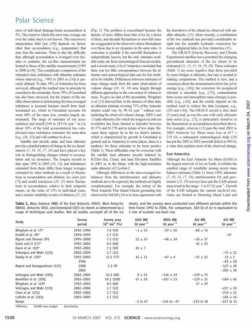
Table 1. Mass balance (MB) of the East Antarctic (EAIS), West Antarctic(WAIS), Antarctic (AIS), and Greenland (GIS) ice sheets as determined by arange of techniques and studies. Not all studies surveyed all of the ice

sheets, and the surveys were conducted over different periods within thetime frame 1992 to 2006. For comparison, 360 Gt of ice is equivalent to1 mm of eustatic sea-level rise.

Study Surveyperiod

Survey area106 km2 (%)

EAIS MBGt year−1

WAIS MBGt year−1

AIS MBGt year−1

GIS MBGt year−1

Wingham et al. (7)* 1992–1996 7.6 (54) –1 ± 53 –59 ± 50 –60 ± 76Krabill et al. (8)* 1993–1999 1.7 (12) –47Rignot and Thomas (9)† 1995–2000 7.2 (51) 22 ± 23 –48 ± 14 –26 ± 37Davis and Li (17)* 1992–2002 8.5 (60) 42 ± 23Davis et al. (10)* 1992–2003 7.1 (50) 45 ± 7Velicogna and Wahr (11)‡ 2002–2004 1.7 (12) –75 ± 21Zwally et al. (18)* 1992–2002 11.1 (77) 16 ± 11 –47 ± 4 –31 ± 12 11 ± 3

Rignot and Kanagaratnam (12)†199620002005

1.2 (9)–83 ± 28

–127 ± 28–205 ± 38

Velicogna and Wahr (20)‡ 2002–2005 12.4 (88) 0 ± 51 –136 ± 19 –139 ± 73Ramillien et al. (19)‡ 2002–2005 14.1 (100) 67 ± 28 –107 ± 23 –129 ± 15 –169 ± 66Wingham et al. (14)* 1992–2003 8.5 (60) 27 ± 29Velicogna and Wahr (13)‡ 2002–2006 1.7 (12) –227 ± 33Chen et al. (15)‡ 2002–2005 1.7 (12) –219 ± 21Luthcke et al. (16)‡ 2003–2005 1.7 (12) –101 ± 16Range –1 to 67 –136 to –47 –139 to 42 –227 to 11*Altimetry. †InSAR mass budget. ‡Gravimetry.

16 MARCH 2007 VOL 315 SCIENCE www.sciencemag.org1530

Polar Science

on

Mar

ch 2

4, 2

007

ww

w.s

cien

cem

ag.o

rgD

ownl

oade

d fr

om

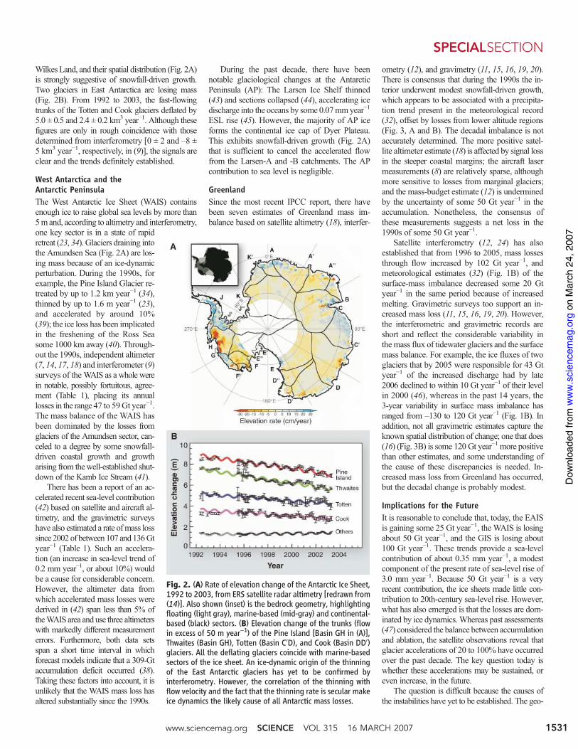
Wilkes Land, and their spatial distribution (Fig. 2A)is strongly suggestive of snowfall-driven growth.Two glaciers in East Antarctica are losing mass(Fig. 2B). From 1992 to 2003, the fast-flowingtrunks of the Totten and Cook glaciers deflated by5.0 ± 0.5 and 2.4 ± 0.2 km3 year−1. Although thesefigures are only in rough coincidence with thosedetermined from interferometry [0 ± 2 and –8 ±5 km3 year−1, respectively, in (9)], the signals areclear and the trends definitely established.

West Antarctica and theAntarctic PeninsulaThe West Antarctic Ice Sheet (WAIS) containsenough ice to raise global sea levels by more than5m and, according to altimetry and interferometry,one key sector is in a state of rapidretreat (23, 34). Glaciers draining intothe Amundsen Sea (Fig. 2A) are los-ing mass because of an ice-dynamicperturbation. During the 1990s, forexample, the Pine Island Glacier re-treated by up to 1.2 km year−1 (34),thinned by up to 1.6 m year−1 (23),and accelerated by around 10%(39); the ice loss has been implicatedin the freshening of the Ross Seasome 1000 km away (40). Through-out the 1990s, independent altimeter(7, 14, 17, 18) and interferometer (9)surveys of the WAIS as a whole werein notable, possibly fortuitous, agree-ment (Table 1), placing its annuallosses in the range 47 to 59Gt year−1.The mass balance of the WAIS hasbeen dominated by the losses fromglaciers of the Amundsen sector, can-celed to a degree by some snowfall-driven coastal growth and growtharising from thewell-established shut-down of the Kamb Ice Stream (41).

There has been a report of an ac-celerated recent sea-level contribution(42) based on satellite and aircraft al-timetry, and the gravimetric surveyshave also estimated a rate ofmass losssince 2002 of between107 and136Gtyear−1 (Table 1). Such an accelera-tion (an increase in sea-level trend of0.2 mm year−1, or about 10%) wouldbe a cause for considerable concern.However, the altimeter data fromwhich accelerated mass losses werederived in (42) span less than 5% oftheWAIS area and use three altimeterswith markedly different measurementerrors. Furthermore, both data setsspan a short time interval in whichforecast models indicate that a 309-Gtaccumulation deficit occurred (38).Taking these factors into account, it isunlikely that the WAIS mass loss hasaltered substantially since the 1990s.

During the past decade, there have beennotable glaciological changes at the AntarcticPeninsula (AP): The Larsen Ice Shelf thinned(43) and sections collapsed (44), accelerating icedischarge into the oceans by some 0.07mmyear−1

ESL rise (45). However, the majority of AP iceforms the continental ice cap of Dyer Plateau.This exhibits snowfall-driven growth (Fig. 2A)that is sufficient to cancel the accelerated flowfrom the Larsen-A and -B catchments. The APcontribution to sea level is negligible.

GreenlandSince the most recent IPCC report, there havebeen seven estimates of Greenland mass im-balance based on satellite altimetry (18), interfer-

ometry (12), and gravimetry (11, 15, 16, 19, 20).There is consensus that during the 1990s the in-terior underwent modest snowfall-driven growth,which appears to be associated with a precipita-tion trend present in the meteorological record(32), offset by losses from lower altitude regions(Fig. 3, A and B). The decadal imbalance is notaccurately determined. The more positive satel-lite altimeter estimate (18) is affected by signal lossin the steeper coastal margins; the aircraft lasermeasurements (8) are relatively sparse, althoughmore sensitive to losses from marginal glaciers;and the mass-budget estimate (12) is underminedby the uncertainty of some 50 Gt year−1 in theaccumulation. Nonetheless, the consensus ofthese measurements suggests a net loss in the1990s of some 50 Gt year−1.

Satellite interferometry (12, 24) has alsoestablished that from 1996 to 2005, mass lossesthrough flow increased by 102 Gt year−1, andmeteorological estimates (32) (Fig. 1B) of thesurface-mass imbalance decreased some 20 Gtyear−1 in the same period because of increasedmelting. Gravimetric surveys too support an in-creased mass loss (11, 15, 16, 19, 20). However,the interferometric and gravimetric records areshort and reflect the considerable variability inthemass flux of tidewater glaciers and the surfacemass balance. For example, the ice fluxes of twoglaciers that by 2005 were responsible for 43 Gtyear−1 of the increased discharge had by late2006 declined to within 10 Gt year−1 of their levelin 2000 (46), whereas in the past 14 years, the3-year variability in surface mass imbalance hasranged from –130 to 120 Gt year−1 (Fig. 1B). Inaddition, not all gravimetric estimates capture theknown spatial distribution of change; one that does(16) (Fig. 3B) is some 120 Gt year−1 more positivethan other estimates, and some understanding ofthe cause of these discrepancies is needed. In-creased mass loss from Greenland has occurred,but the decadal change is probably modest.

Implications for the FutureIt is reasonable to conclude that, today, the EAISis gaining some 25 Gt year−1, the WAIS is losingabout 50 Gt year−1, and the GIS is losing about100 Gt year−1. These trends provide a sea-levelcontribution of about 0.35 mm year−1, a modestcomponent of the present rate of sea-level rise of3.0 mm year−1. Because 50 Gt year−1 is a veryrecent contribution, the ice sheets made little con-tribution to 20th-century sea-level rise. However,what has also emerged is that the losses are dom-inated by ice dynamics.Whereas past assessments(47) considered the balance between accumulationand ablation, the satellite observations reveal thatglacier accelerations of 20 to 100% have occurredover the past decade. The key question today iswhether these accelerations may be sustained, oreven increase, in the future.

The question is difficult because the causes ofthe instabilities have yet to be established. The geo-

Fig. 2. (A) Rate of elevation change of the Antarctic Ice Sheet,1992 to 2003, from ERS satellite radar altimetry [redrawn from(14)]. Also shown (inset) is the bedrock geometry, highlightingfloating (light gray), marine-based (mid-gray) and continental-based (black) sectors. (B) Elevation change of the trunks (flowin excess of 50 m year−1) of the Pine Island [Basin GH in (A)],Thwaites (Basin GH), Totten (Basin C′D), and Cook (Basin DD′)glaciers. All the deflating glaciers coincide with marine-basedsectors of the ice sheet. An ice-dynamic origin of the thinningof the East Antarctic glaciers has yet to be confirmed byinterferometry. However, the correlation of the thinning withflow velocity and the fact that the thinning rate is secular makeice dynamics the likely cause of all Antarctic mass losses.

www.sciencemag.org SCIENCE VOL 315 16 MARCH 2007 1531

SPECIALSECTION

on

Mar

ch 2

4, 2

007

ww

w.s

cien

cem

ag.o

rgD

ownl

oade

d fr

om

logical record (48) suggests that some10,000 years ago, the Amundsensector of the WAIS extended only100 km farther than today, confiningthe present rate of retreat to morerecent times, and the drawdown ofthe Amundsen sector ice streamshas been linked (49) to a recent triggerin the ocean. A comparable argumentmay be extended to the thinning gla-ciers in East Antarctica andGreenland,which are also marine terminated.Equally, there is no direct evidenceof a warming of the Amundsen Sea,and it has long been held possible thatthe marine-terminatedWAIS, and theAmundsen sector in particular, maybe geometrically unstable (50), andthe retreating East Antarctica streamshave a similar geometry (Fig. 2A). InGreenland, where summermelting iswidespread and increasing,Global Po-sitioning System measurements haveshown the melting to affect flow ve-locity in the ice sheet interior (26), in-troducing the possibility that increasedsurface meltwater is reaching thebed and accelerating the ice flow tothe ocean.

The discovery that particular icestreams and glaciers are dominatingice sheet mass losses means thattoday our ability to predict futurechanges is limited. Present numericalmodels capture neither the details ofactual ice streams nor, in Greenland,those of hydraulic connections be-tween the surface and the bed. Inaddition, the detailed mechanics atthe grounding line still remain to befully worked out. In consequence,the view that the changing sea-levelcontribution of the Antarctic andGreenland ice sheets in the 21st cen-tury will be both small and negativeas a result of accumulating snow inAntarctica [e.g., –0.05 mm year−1 in(1)] is now uncertain.

Because our predictive ability islimited, continued observation isessential. The satellite record clearlyidentifies the particular ice streamsand glaciers whose evolution is of greatestconcern. The causes of their instability need tobe identified. Their detailed basal topography,their basal hydrology, and the details of the in-teraction with their surrounding shelf seas needto be established. Numerical models that cap-ture the detailed dynamics of these glaciers andtheir hydrology are required. Of equal impor-tance are meteorological and ice core measure-ments that will increase confidence in forecastmodels of accumulation and ablation fluctuations,

because to a considerable extent these limitinterpretations of the short satellite records. Thereis a great deal that the International Polar Yearmay achieve.

References and Notes1. J. A. Church, J. M. Gregory, in Climate Change 2001: The

Scientific Basis, J. T. Houghton et al., Eds. (CambridgeUniv. Press, Cambridge, 2001), chap. 11, pp. 641–693.

2. R. G. Fairbanks, Nature 342, 637 (1989).3. N. Stern, The Economics of Climate Change: The Stern

Review (Cambridge Univ. Press, Cambridge, 2006).

4. C. S. Benson, “Stratigraphic studies in the snow and firn ofGreenland ice sheet” Research Report 70 (Cold RegionsResearch and Engineering Lab, Hanover, NH, 1962).

5. C. R. Bentley, M. B. Giovinetto, Proceedings of theInternational Conference on the Role of Polar Regions inGlobal Change (Geophysical Institute, University ofAlaska, Fairbanks, AK, 1991), pp. 481–486.

6. S. S. Jacobs, Nature 360, 29 (1992).7. D. J. Wingham, A. Ridout, R. Scharroo, R. Arthern,

C. K. Shum, Science 282, 456 (1998).8. W. Krabill et al., Science 289, 428 (2000).9. E. Rignot, R. H. Thomas, Science 297, 1502 (2002).

10. C. H. Davis, Y. Li, J. R. McConnell, M. M. Frey, E. Hanna,Science 308, 1898 (2005).

11. I. Velicogna, J. Wahr, Geophys. Res. Lett. 32, art-L18505(2005).

12. E. Rignot, P. Kanagaratnam, Science 311, 986 (2006).13. I. Velicogna, J. Wahr, Science 311, 1754 (2006).14. D. J. Wingham, A. Shepherd, A. Muir, G. J. Marshall,

Philos. Trans. R. Soc. A Math. Phys. Eng. Sci. 364, 1627(2006).

15. J. L. Chen, C. R. Wilson, B. D. Tapley, Science 313, 1958(2006).

16. S. B. Luthcke et al., Science 314, 1286 (2006).17. C. H. Davis, Y. H. Li, paper presented at Science for Society:

Exploring and Managing a Changing Planet (IEEE,Anchorage, Alaska, 20–24 Sep 2004), pp. 1152–1155.

18. H. J. Zwally et al., J. Glaciol. 51, 509 (2005).19. G. Ramillien et al., Global Planet. Change 53, 198 (2006).20. I. Velicogna, J. Wahr, Nature 443, 329 (2006).21. W. Munk, Science 300, 2041 (2003).22. O. M. Johannessen, K. Khvorostovsky, L. P. Bobylev,

Science 310, 1013 (2005).23. A. Shepherd, D. J. Wingham, J. A. D. Mansley, H. F. J.

Corr, Science 291, 862 (2001).24. I. Joughin, W. Abdalati, M. Fahnestock, Nature 432, 608

(2004).25. A. Luckman, T. Murray, R. de Lange, E. Hanna, Geophys.

Res. Lett. 33, art-L03503 (2006).26. H. J. Zwally et al., Science 297, 218 (2002).27. R. Bindschadler, Science 311, 1720 (2006).28. A. J. Monaghan, D. H. Bromwich, S. H. Wang, Philos.

Trans. R. Soc. A Math. Phys. Eng. Sci. 364, 1683 (2006).29. R. J. Arthern, D. P. Winebrenner, D. G. Vaughan,

J. Geophys. Res. Atmos. 111, D06107 (2006).30. E. J. Rignot, S. P. Gogineni, W. B. Krabill, S. Ekholm,

Science 276, 934 (1997).31. N. Reeh, H. H. Thomsen, O. B. Olesen, W. Starzer,

Science 278, 205 (1997).32. J. E. Box et al., J. Clim. 19, 2783 (2006).33. N. P. M. van Lipzig, E. van Meijgaard, J. Oerlemans, Int. J.

Climatol. 22, 1197 (2002).34. E. J. Rignot, Science 281, 549 (1998).35. D. J. Wingham, M. J. Siegert, A. Shepherd, A. S. Muir,

Nature 440, 1033 (2006).36. M. Horwath, R. Dietrich, Geophys. Res. Lett. 33,

art-L07502 (2005).37. M. Nakada et al., Mar. Geol. 167, 85 (2000).38. A. J. Monaghan et al., Science 313, 827 (2006).39. I. Joughin, E. Rignot, C. E. Rosanova, B. K. Lucchitta,

J. Bohlander, Geophys. Res. Lett. 30, 1706 (2003).40. S. S. Jacobs, C. F. Giulivi, P. A. Mele, Science 297, 386 (2002).41. S. Anandakrishnan, R. B. Alley, Geophys. Res. Lett. 24,

265 (1997).42. R. Thomas et al., Science 306, 255 (2004).43. A. Shepherd, D. Wingham, T. Payne, P. Skvarca, Science

302, 856 (2003).44. H. Rott, P. Skvarca, T. Nagler, Science 271, 788 (1996).45. E. Rignot et al., Geophys. Res. Lett. 31, art-L18401 (2004).46. I. M. Howat, I. Joughin, T. A. Scambos, Science 315, 1559

(2007).47. R. B. Alley, P. U. Clark, P. Huybrechts, I. Joughin, Science

310, 456 (2005).48. A. L. Lowe, J. B. Anderson, Quat. Sci. Rev. 21, 1879 (2002).49. A. J. Payne, A. Vieli, A. P. Shepherd, D. J. Wingham,

E. Rignot, Geophys. Res. Lett. 31, art-L23401 (2004).50. J. Weertman, J. Glaciol. 13, 3 (1974).

10.1126/science.1136776

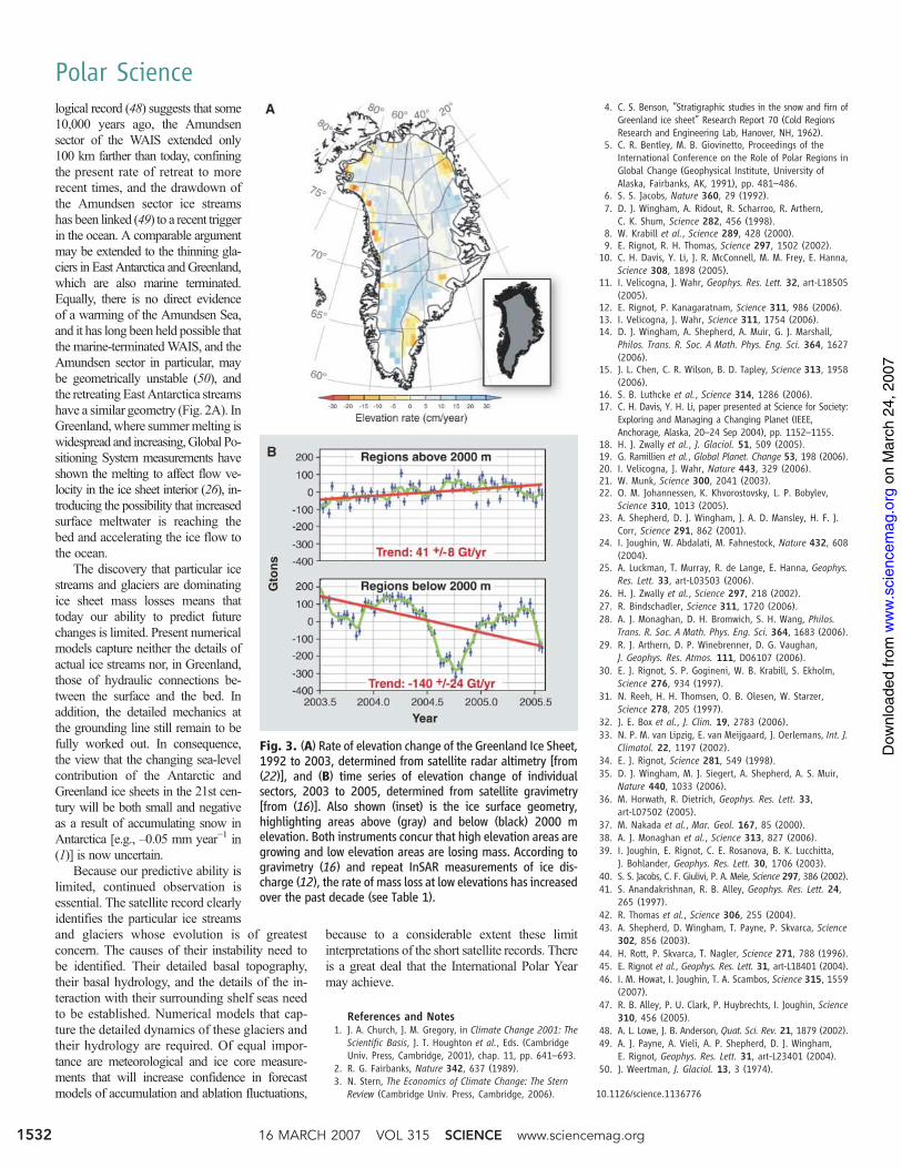
Fig. 3. (A) Rate of elevation change of the Greenland Ice Sheet,1992 to 2003, determined from satellite radar altimetry [from(22)], and (B) time series of elevation change of individualsectors, 2003 to 2005, determined from satellite gravimetry[from (16)]. Also shown (inset) is the ice surface geometry,highlighting areas above (gray) and below (black) 2000 melevation. Both instruments concur that high elevation areas aregrowing and low elevation areas are losing mass. According togravimetry (16) and repeat InSAR measurements of ice dis-charge (12), the rate of mass loss at low elevations has increasedover the past decade (see Table 1).

16 MARCH 2007 VOL 315 SCIENCE www.sciencemag.org1532

Polar Science

on

Mar

ch 2

4, 2

007

ww

w.s

cien

cem

ag.o

rgD

ownl

oade

d fr

om

Rapid Changes in Ice Discharge fromGreenland Outlet GlaciersIan M. Howat,1,2* Ian Joughin,1 Ted A. Scambos2

Using satellite-derived surface elevation and velocity data, we found major short-term variations inrecent ice discharge and mass loss at two of Greenland’s largest outlet glaciers. Their combinedrate of mass loss doubled in less than a year in 2004 and then decreased in 2006 to near theprevious rates, likely as a result of fast re-equilibration of calving-front geometry after retreat.Total mass loss is a fraction of concurrent gravity-derived estimates, pointing to an alternativesource of loss and the need for high-resolution observations of outlet dynamics and glaciergeometry for sea-level rise predictions.

The recent, marked increase in ice dis-charge from many of Greenland’s largeoutlet glaciers has upended the con-

ventional view that variations in ice-sheet massbalance are dominated on short time scales byvariations in surface balance, rather than icedynamics. Beginning in the late 1990s and con-tinuing through the past several years, the ice-flow speed of many tidewater outlet glacierssouth of 72° North increased by up to 100%,increasing the ice sheet’s contribution to sea-level rise by more than 0.25 mm/year (1). Thesynchronous and multiregional scale of thischange and the recent increase in Arctic air andocean temperatures suggest that these changesare linked to climate warming. The possibilitythat ice dynamics are so highly sensitive to cli-mate change is of concern, because the physicalprocesses that would drive such a relationshipare poorly understood and are not realisticallyincluded in ice-sheet models used to predictrates of sea-level rise.

Current estimates of change in Greenland’sice discharge are based on velocity mea-surements taken 4 to 5 years apart (1). How-ever, 50 to 100% increases in ice speed andthinning of tens of meters over a single year havebeen documented in Greenland and elsewhere(2–6). Therefore, discharge should be highly var-iable as well, even at subannual time scales.Large increases in tidewater glacier speed havebeen attributed to decreased flow resistance andincreased along-flow stresses during retreat ofthe ice front (2, 3, 7). This suggests that changesin velocity and discharge are coupled to changesin tidewater glacier geometry and that the ob-served rapid changes may be a transient re-sponse to disequilibrium at the front. Therefore,accurate estimates of current rates of dischargeand the potential for near-future change requireobservations of outlet glacier geometry andspeed at high temporal resolution.

To assess short-term variability in outletglacier dynamics, we examined speed, geometry,and discharge at two of Greenland’s three largestoutlet glaciers between 2000 and 2006. Locatedon the central east coast, Kangerdlugssuaq (KL)and Helheim (HH) represent 35% of eastGreenland’s total discharge (1). The calvingfronts of both glaciers appeared relatively stablefrom the mid-20th century (8, 9) until 2002,when HH retreated more than 7 km in 3 years(2). This was followed by a 5-km retreat of KLduring the winter of 2004 to 2005 (4). Theseretreats are much greater than the 1- to 2-kmseasonal fluctuations previously observed (4, 5)

and followed a sustained period of low-elevationice thinning (8, 10). Retreats were concurrentwith accelerated ice flow (1, 2). This accelera-tion increased rates of mass loss by 28 and 15Gt/year at KL and HH, respectively, between2000 and 2005, representing >40% of the icesheet’s increase in mass loss (1).

We measured summer surface speed and ele-vation for these glaciers using imagery acquiredby the Advanced Spaceborne Thermal Emissionand Reflection radiometer (ASTER) sensoraboard the Terra satellite, launched in 1999.We constructed Photogrammetric Digital Eleva-tion Models (DEMs) from ASTER stereobands(3N and 3B) and validated them (Figs. 1D and2D) using laser altimetry data sets collected byNASA’s Airborne Topographic Mapper (ATM)in 2001, 2003, and 2005 (10). The root-mean-squared differences between DEM and ATMelevations are 10 m, which is similar to the un-certainty quoted in ASTER DEM validationstudies (11) (Figs. 1D and 2D). Summer surfacevelocity was obtained from automated featuretracking between repeat, orthorectified principalcomponent images of bands 1 to 3 (2, 12). Un-certainty in these measurements is ~5 m perimage pair, or 0.1 to 0.8 m/day for the datapresented here. We determined winter velocities(±3% uncertainty) using radar speckle trackingbetween Canadian Space Agency Radar Satellite

Fig. 1. KL glacier. (A) Surface elevation (zs) from (solid) ASTER DEMs and (dashed) Airborne ATM laseraltimetry and bed elevation (zb) from CoRDS. (B) Surface velocity obtained from (solid) optical featuretracking and (dashed) radar speckle tracking along the main flow line, denoted by white dashes in (D).Arrows point to location of flux gate used for discharge calculation. (C) Elevation change along the sameprofile. Dashed segments are changes due to movement of the ice front. (D) Maps of elevation changefrom differenced ASTER DEMs overlaid on the 21 June 2005 image. Circles show repeat ATM altimetrymeasurements for the same time period and x marks flux-gate location. Error bars in (B) and (C) showmeans ± SD.

1Polar Science Center, Applied Physics Lab, University ofWashington, 1013 Northeast 40th Street, Seattle, WA98105–6698, USA. 2National Snow and Ice Data Center,University of Colorado, 1540 30th Street, Boulder, CO,80309–0449, USA.

*To whom correspondence should be addressed. E-mail:ihowat@apl.washington.edu

www.sciencemag.org SCIENCE VOL 315 16 MARCH 2007 1559

REPORTS

on

Mar

ch 2

4, 2

007

ww

w.s

cien

cem

ag.o

rgD

ownl

oade

d fr

om

(RADARSAT) image pairs (24-day separation)(13). In some cases, combinations of multipleelevation and speed data sets from the sameseason improved spatial coverage and reducederrors. The University of Kansas Coherent RadarDepth Sounder (CoRDS) surveyed ice thicknessand bed elevation at both glaciers in 2001 (14).

From summer 2004 to spring 2005, KL re-treated by 5 km (4), and its speed increased by80% near the front and by ~20% at 30 km inland(Fig. 1). Between April and July 2005, the in-crease in speed migrated rapidly inland with a~5% decrease in speed close to the front and a~7% increase in speed in areas farther inland (up-glacier). This upstream propagation continuedfrom July 2005 through July 2006, with the near-front deceleration of ~15% and up-glacieracceleration of ~25%, with the transition betweenspeedup and slowdown at ~15 km. The glacierthinned rapidly during acceleration, with 80 mof thinning near the front and thinning of at least40 m extending 40 km inland by summer 2005.Thinningmoved inland between 2005 and 2006,with a peak thinning of 68 m at about 26 km, butwith virtually no thinning at the front. Averagethinning over the glacier during the summer of2006 declined to near zero, with some apparentthickening in areas on the main trunk.

Images from June 2003 are the first to in-dicate substantial retreat (2.1 km) at HH. Duringadditional retreat over that summer, speedup of20 to 40% extended at least 20 km up-glacier(Fig. 2). The ice front and speed changed little in2004, but 4 km of new retreat yielded anothermajor speedup (25%) in the summer of 2005.Many of the earlier data do not extend far inland,but echoing the pattern on KL, speeds from2006 show a progressive inland accelerationaccompanied by deceleration (25%) extendingfrom about 15 km toward the ice front. As withKL, rapid thinning accompanied the large speedincreases. By late summer 2006, strain ratesindicate a region of compression at about 12 to15 km. The initial HH acceleration in 2003produced 40 m of thinning within about 15 kmof the ice front. This thinning slowed to 10 m/yearwhen there was little retreat from 2003 to 2004.The 4-km retreat from 2004 to 2005 moved theice front over a 200-m bathymetric depression,bringing it to or near flotation. Between thesummers of 2005 and 2006, the rate of thin-ning decreased within 20 km of the front, reach-ing zero at the front and increasing to 50 m/year25 km from the front. During this period, theglacier advanced 4 km as a floating or near-floating tongue to near the 2003–2004 frontposition. It appears that the front of this floatingtongue may have regrounded in summer 2006,contributing to the deceleration and the region ofcompression.

On both KL and HH, the data show a mark-edly similar progression of increasing down-glacier speed and thinning synchronous withretreat, followed by an inland migration of thespeed increase. As the front restabilized, speed

and thinning increased up-glacier and decreaseddown-glacier. This progression of dynamic re-sponse strongly suggests that the notable in-creases in acceleration and thinning are relatedto changes in calving-front position through var-iations in longitudinal stresses (2). Consistentwith standard theories of tidewater glacier dy-namics (15), rapid retreat at HH occurred as thefront moved into deeper water and stoppedwhere the bed slope reversed (Fig. 2). At bothglaciers, the initial acceleration and thinning af-ter retreat were concentrated within 10 to 20 kmof the ice front, which would be the expectedrange of stress coupling (16). Relative thinningdown-glacier increases the surface slope anddriving stress up-glacier. By thismeans, thinningand acceleration are advected up-glacier (17).

This can be seen at KL, where the maximumthinning rates moved ~10 km up-glacier be-tween 2005 and 2006 (Fig. 1). This propagationrate is equal to about five times the distance-integrated 2005 ice speed, which is the approx-imate rate of advection of a kinematic wavetraveling through ice (18).

We estimated discharge anomalies relativeto the year 2000, when the glaciers were nearbalance, taking into account the changes in bothspeed and thickness (Fig. 3). At each glacier,our discharge estimates from 2000 to 2005 agreeclosely with mass-budget estimates (1). At KL,roughly 80% of the total increase in dischargeoccurred in less than 1 year in 2005, followed bya 25% drop the next year (Fig. 3). At HH, dis-charge increased 5 Gt/year between 2000 and

Fig. 2. (A to D) Same as Fig. 1 for HH, except (D) uses a 29 August 2005 image background.

Fig. 3. Discharge anomaly fromyear 2000. Circles with error barsare calculated from speed andthickness change across flux gatesshown in Figs. 1 and 2 with initialice thickness obtained by dividingthe year 2000 flux by the productof glacier width and 2000 speed(1). Uncertainties are the combi-nations of errors in ice elevationand speed. Triangles are the dis-charge anomaly with ice thicknessheld constant. Diamonds are the2000 to 2005 discharge-changevalues from mass budget (1). Rect-angles are KL mass-loss estimatesfrom differencing repeat on-iceASTER DEMs over the area shown in Fig. 1D. Spatial DEM coverage for HH is incomplete, preventingmass-loss calculations. The horizontal ranges in these estimates are the image acquisition dates, and thevertical range is the uncertainty.

16 MARCH 2007 VOL 315 SCIENCE www.sciencemag.org1560

REPORTS

on

Mar

ch 2

4, 2

007

ww

w.s

cien

cem

ag.o

rgD

ownl

oade

d fr

om

2003 and by another 7 Gt/year between 2004and 2005. It then dropped bymore than 13Gt/yearin 2006, returning to near its 2000 value.

Integrating the time series of discharge anom-aly from 2000 to 2006 gives totals of 52 Gt atKL and 30 Gt of excess discharge at HH (Fig. 3).Extensive DEM coverage of KL allows for adirect estimate of volume change over the lowerbasin (47 Gt), excluding any additional thinningat higher elevation. This loss estimate (47 Gt)agrees well with the KL discharge anomaly.When the existing imbalances from 2000 arefactored in, the combined net loss of ice from2000 to 2006 is 90 Gt, with 63 Gt of this loss inthe interval from summer 2004 to summer 2006.The sharp increase in mass loss through theseglaciers between 2004 and 2005 (32 Gt) canexplain about 30% of the mass loss indicated byGravity Recovery and Climate Experiment(GRACE) gravity observations for southeastGreenland (19).

Other GRACE observations suggest a 450 Gtice loss from southGreenland betweenMay 2004andApril 2006 that the authorsmostly attribute toincreased discharge from HH and KL (20).Although the timing of the increased loss agreeswell with the KL andHH acceleration, our resultssuggest that the combined loss from these glaciersover this period can only account for 13% of thisloss. Absent an extensive but unobserved accel-eration elsewhere, measurements for other southGreenland glaciers suggest a loss increase from2000 to 2005 of roughly 23 Gt/year (1). Thissuggests that despite large dynamic changes,much of the loss between 2004 and 2006estimated fromGRACEmay be related to surfacebalance anomalies or other causes.

Our results indicate that large variations inoutlet glacier discharge can produce large dis-charge anomalies in a span of a few years.Although the initial triggering for the recent

changes is unclear, it is well known that verysmall perturbations to thickness can induce re-treat in calving glaciers (15). In the cases we ex-amined, large imbalances appear to have causedrapid adjustments in the glacier geometry,leading to a quick (~2-year) return to near ba-lance, though some degree of moderate thinningmay persist. The surface drawdown of 100 m ormore at low elevations within the outlets mayhave substantial effects on summertime surfacemelt rates, potentially predisposing them tofurther ice thinning and retreat. However, predic-tion of near-future change will require detaileddata on bed elevation and ice thickness. This isnot yet available for most of the outlet glaciers.

Dynamic re-equilibration after a perturbationin geometry may not always be as rapid as ob-served here. For example, Jakobshavn Isbrae hasmaintained high speeds for several years afterretreat and acceleration (fig. S1) (3). In this case,retreat from the fjord increased inflow from thesides, potentially resulting in lower thinningrates (~15 m/year) (5, 10). Likewise, manyglaciers along Greenland’s northwest coast haveretreated into the ice sheet with sustainedthinning at rates of a few meters per year butshow no apparent change in speed (1). Thissuggests that geometry and other characteristicsunique to each glacier may determine the timescale over which discharge anomalies occur.

The highly variable dynamics of outlet gla-ciers suggest that special care must be taken inhow mass-balance estimates are evaluated, par-ticularly when extrapolating into the future,because short-term spikes could yield erroneouslong-term trends. Rather than yielding a well-defined trend, our results are notable in that theyshow that Greenland mass balance can fluctuaterapidly. If these changes are the result of recentwarm summers (21), continued warming maycause a long-term drawdown of the ice sheet

through a series of such discharge anomalies,perhaps with a similar degree of variability. There-fore, accurate estimates of ice-sheet mass balancewill require subannual observations of outletglacier dynamics to avoid aliasing this rapidlyvarying signal.

References and Notes1. E. Rignot, P. Kanagaratnam, Science 311, 986 (2006).2. I. M. Howat, I. Joughin, S. Tulaczyk, P. Gogineni,

Geophys. Res. Lett. 32, L22502 (2005).3. I. Joughin, W. Abdalati, M. Fahnestock, Nature 432, 608

(2004).4. A. Luckman, A. Murray, R. De Lange, E. Hanna, Geophys.

Res. Lett. 33, L03503 (2006).5. R. H. Thomas et al., J. Glaciol. 49, 231 (2003).6. T. A. Scambos, J. A. Bohlander, C. A. Shuman, P. Skvarca,

Geophys. Res. Lett. 31, L18402 (2004).7. R. H. Thomas, J. Glaciol. 50, 57 (2004).8. R. H. Thomas et al., Geophys. Res. Lett. 27, 1291 (2000).9. A. Weidick, U.S. Geol. Surv. Prof. Pap. 386-C (1995),

pp. C85–C87.10. W. Krabill et al., Geophys. Res. Lett. 31, L24402 (2004).11. B. T. San, M. L. Suzen, Int. J. Remote Sens. 26, 5013 (2005).12. T. A. Scambos, M. J. Dutkiewicz, J. C. Wilson,

R. A. Bindschadler, Remote Sens. Environ. 42, 177 (1992).13. I. Joughin, Ann. Glaciol. 34, 195 (2002).14. S. Gogineni et al., J. Geophys. Res. 106, 33761 (2001).15. M. F. Meier, A. Post, J. Geophys. Res. 92, 9051 (1987).16. B. Kamb, K. A. Echelmeyer, J. Glaciol. 32, 267 (1986).17. A. J. Payne, A. Vieli, A. P. Shepherd, D. J. Wingham,

E. Rignot, Geophys. Res. Lett. 31, L23401 (2004).18. C. J. Van der Veen, in Fundamentals of Glacier Dynamics

(A. A. Balkema, Rotterdam, Netherlands, 1999), p. 313.19. S. B. Luthcke et al., Science 314, 1286 (2006).20. I. Velicogna, J. Wahr, Nature 443, 329 (2006).21. I. Joughin, Science 311, 1719 (2006).22. NASA grants NNG06GE5SG and NNG06GE50G supported

the contribution of I.M.H. and T.A.S. NSF grantARC-0531270 supported I.R.J.’s contribution.

Supporting Online Materialwww.sciencemag.org/cgi/content/full/1138478/DC1Fig. S1Reference

6 December 2006; accepted 24 January 2007Published online 8 February 2007;10.1126/science.1138478Include this information when citing this paper.

Conformationally ControlledChemistry: Excited-State DynamicsDictate Ground-State ReactionMyung Hwa Kim,1,2 Lei Shen,1 Hongli Tao,3 Todd J. Martinez,3* Arthur G. Suits1,2*

Ion imaging reveals distinct photodissociation dynamics for propanal cations initially prepared ineither the cis or gauche conformation, even though these isomers differ only slightly in energyand face a small interconversion barrier. The product kinetic energy distributions for the hydrogenatom elimination channels are bimodal, and the two peaks are readily assigned to propanoylcation or hydroxyallyl cation coproducts. Ab initio multiple spawning dynamical calculationssuggest that distinct ultrafast dynamics in the excited state deposit each conformer in isolatedregions of the ground-state potential energy surface, and, from these distinct regions, conformerinterconversion does not effectively compete with dissociation.

From stereoselective synthesis to proteinfolding, conformational dynamics lie atthe heart of chemistry (1). Molecular

conformers typically interconvert via hinderedrotations about single bonds, and the low en-ergy barriers to these processes lead to equil-

ibration even at low temperatures. Recentefforts to explore the detailed conformationalenergy landscapes of molecules have relied onstimulated emission pumping in jet-cooledbeams, exciting then re-trapping molecules indifferent local minima to probe the intercon-version barriers (2, 3). Single-molecule methodshave also been used to investigate conforma-tional heterogeneity: Otherwise identical mole-cules exhibit vastly different rates in key stepsof enzymatic processes (4, 5). Conformationalselectivity has been suggested as a means ofachieving laser control of chemical outcomes(6). However, the low barriers for intercon-

1Department of Chemistry, Wayne State University, Detroit,MI 48202, USA. 2Department of Chemistry, Stony BrookUniversity, Stony Brook, NY 11794, USA. 3Department ofChemistry, University of Illinois, Champaign, IL 61801,USA.

*To whom correspondence should be addressed. E-mail:asuits@chem.wayne.edu (A.G.S.); tjm@spawn.scs.uiuc.edu(T.J.M.)

www.sciencemag.org SCIENCE VOL 315 16 MARCH 2007 1561

REPORTS

on

Mar

ch 2

4, 2

007

ww

w.s

cien

cem

ag.o

rgD

ownl

oade

d fr

om