lable at ScienceDirect

Atmospheric Environment 107 (2015) 70e84

Contents lists avai

Atmospheric Environment

journal homepage: www.elsevier .com/locate/atmosenv

Long-term NOx trends over large cities in the United States during thegreat recession: Comparison of satellite retrievals, groundobservations, and emission inventories

Daniel Q. Tong a, b, c, *, Lok Lamsal d, e, Li Pan a, b, Charles Ding a, f, Hyuncheol Kim a, b,Pius Lee a, Tianfeng Chai a, b, Kenneth E. Pickering e, Ivanka Stajner g

a NOAA Air Resources Laboratory (ARL), NOAA Center for Weather and Climate Prediction, 5830 University Research Court, College Park, MD 20740, USAb Cooperative Institute for Climate and Satellites, University of Maryland, College Park, MD 20740, USAc Center for Spatial Information Science and Systems (CSISS), George Mason University, Fairfax, VA 22030, USAd Goddard Earth Sciences Technology and Research, Universities Space Research Association, Columbia, MD, USAe NASA Goddard Space Flight Center, Greenbelt, MD, USAf University of California at Berkeley, Berkeley, CA, USAg NOAA National Weather Service, Silver Spring, MD 20910, USA

h i g h l i g h t s

� Derived multi-year urban NOx trend from satellite (OMI) and ground observations (AQS).� Revealed NOx responses to the 2008 Economic Recession by OMI and AQS.� The trend not well captured by emissions used for national air quality forecasting.� Demonstrated how to use space and ground observations to evaluate emission updates.

a r t i c l e i n f o

Article history:Received 11 April 2014Received in revised form2 January 2015Accepted 14 January 2015Available online 15 January 2015

Keywords:NOx

EmissionTrendAir quality forecastRecessionOMI NO2OzoneAQSNAQFC

* Corresponding author. NOAA Air Resources LaborWeather and Climate Prediction, 5830 University Rese20740, USA.

E-mail address: Daniel.Tong@noaa.gov (D.Q. Tong)

http://dx.doi.org/10.1016/j.atmosenv.2015.01.0351352-2310/© 2015 The Authors. Published by Elsevier

a b s t r a c t

National emission inventories (NEIs) take years to assemble, but they can become outdated quickly,especially for time-sensitive applications such as air quality forecasting. This study compares multi-yearNOx trends derived from satellite and ground observations and uses these data to evaluate the updates ofNOx emission data by the US National Air Quality Forecast Capability (NAQFC) for next-day ozone pre-diction during the 2008 Global Economic Recession. Over the eight large US cities examined here, boththe Ozone Monitoring Instrument (OMI) and the Air Quality System (AQS) detect substantial downwardtrends from 2005 to 2012, with a seven-year total of �35% according to OMI and �38% according to AQS.The NOx emission projection adopted by NAQFC tends to be in the right direction, but at a slowerreduction rate (�25% from 2005 to 2012), due likely to the unaccounted effects of the 2008 economicrecession. Both OMI and AQS datasets display distinct emission reduction rates before, during, and afterthe 2008 global recession in some cities, but the detailed changing rates are not consistent across theOMI and AQS data. Our findings demonstrate the feasibility of using space and ground observations toevaluate major updates of emission inventories objectively. The combination of satellite, ground obser-vations, and in-situ measurements (such as emission monitoring in power plants) is likely to providemore reliable estimates of NOx emission and its trend, which is an issue of increasing importance asmany urban areas in the US are transitioning to NOx-sensitive chemical regimes by continuous emissionreductions.© 2015 The Authors. Published by Elsevier Ltd. This is an open access article under the CC BY-NC-ND

license (http://creativecommons.org/licenses/by-nc-nd/4.0/).

atory (ARL), NOAA Center forarch Court, College Park, MD

.

Ltd. This is an open access article u

1. Introduction

Nitrogen oxides (NOx ¼ NO þ NO2) are key precursors totropospheric ambient ozone (O3) and fine particulate matter(PM2.5) (Crutzen and Gidel, 1983; Spicer, 1983), which has been

nder the CC BY-NC-ND license (http://creativecommons.org/licenses/by-nc-nd/4.0/).

D.Q. Tong et al. / Atmospheric Environment 107 (2015) 70e84 71

associated with adverse health effects, including respiratory dis-eases and cardiovascular mortality (Pope et al., 2002; Jerrett et al.,2009). As of December 2013, the United States EnvironmentalProtection Agency (US EPA) estimates that more than one-third ofthe US population lives in areas that exceed the national ambientair quality standards (NAAQS) for either O3 or PM2.5 (US EPA, 2014a,2014b). To assist state and local agencies in mitigating the effects ofunhealthy levels of air pollution, the National Air Quality Fore-casting Capability (NAQFC) system (Otte et al., 2005), currentlyoperated by the National Weather Service, was designed to provideair quality forecasting guidance over the contiguous United States,Hawaii, and Alaska for next day forecasts (Stajner et al., 2012). NOxare emitted from both anthropogenic sources (transportation, po-wer plants, and fertilizers) and natural sources (biomass burning,lightning, and soils) (Warneck, 2000). Once emitted, NOx reactswith volatile organic compounds under sunlight to form tropo-spheric ozone (Liu et al., 1987) and particulate nitrate, an importantcomponent of PM2.5. Hence, quantifying the amount of NOx emittedinto the atmosphere is essential for reliable prediction of surfaceozone and PM2.5.

It is often challenging to provide accurate estimates of NOx

emissions for time-sensitive applications such as NAQFC, given therapid progression of emission control and other socioeconomicevents that affect emission loading (e.g., Harley et al., 2005; van derA et al., 2008; Stavrakou et al., 2008; Konovalov et al., 2010; Pinderet al., 2011; Castellanos and Boersma, 2012; Duncan et al., 2013).NAQFC relies on national emission inventories (NEIs) to account forthousands of anthropogenic emission sources and other emissionmodels for natural sources. The substantial cost and effort entailedin collecting data relevant for compiling NEIs are prohibitive forfrequent and timely updates of NOx NEIs using conventionalemission modeling approaches. As a result, the emission data usedin NAQFC are several years behind the forecasting year, imposinguncertainties on air quality forecasting (Tong et al., 2012).

Can satellite-based emission data provide reliable informationin order to rapidly update NOx emission inventories and therebysupport NAQFC-type air quality applications? NO2 retrievals frompolar orbiting satellite sensors such as SCIAMACHYand GOME havebeen used to update anthropogenic NOx emission inventories(Martin et al., 2003; Lamsal et al., 2011; Mijling and van der A,

Fig. 1. Locations of the eight selected metropolitan statistical areas, which are among the memission density based on the NAQFC emission data, with red indicating high NOx emissionreferred to the web version of this article.)

2012). This satellite-based approach, while showing great poten-tial to reduce the emission time lag, has yet to be verified withindependent data sources. To evaluate the robustness of thisapproach, this study thus compares the long-term NO2 trendsderived from the Ozone Monitoring Instrument (OMI) (Boersmaet al., 2007) with the operational emission data used in NAQFCpredictions, with emphasis on both the emission changes betweenmajor updates and the year-to-year progression over eight metro-politan areas from 2005 to 2012. A third data source, the EPA's AQSground observations, serves as an independent reference to helpverify urban NOx trends. Estimation of future year emissions for airquality and climate modeling often relies on emission projections(Bond et al., 2004; Granier et al., 2011). NAQFC emissions areupdated annually based on the available emission inventories,emission measurements, and projections. Rigorous evaluations ofthese annual updates, however, have not been performed regularly,largely because of the lack of observational data to directly verifyemission projections. Meanwhile, AQS data have been used as aproxy for urban emissions since morning rush-hour concentrationsare predominantly influenced by emissions from heavy commutertraffic (Godowitch et al., 2010). The AQS measurements have beencoupled with other data to identify source strength and the originof reactive nitrogen oxides over the Southeastern United States(Tong et al., 2005). Therefore, all three data sources provide inde-pendent quantification of NOx emissions that can be compared overa fixed time period.

The intercomparisons of changes in NOx from NAQFC, OMI, andAQS are expected to serve dual purposes: 1) to compare the NOxtrends derived from space and ground observations; and 2) toevaluate NAQFC emission updates against satellite and groundobservations. We focus here on the NOx trends over eight majormetropolitan areas (Fig. 1) where NOx emission density is high andAQS monitors are abundant. We further concentrate on the NOxtrends during summertime when the NOx photochemical lifetimeis shorter (4 h at noon), the carryover from the previous day islimited and regional transport is at minimal, yielding a column thatis especially representative of local surface emissions (Russell et al.,2010). Further, the number of available satellite measurements ismaximized during summer months, when cloud cover is lowest.Finally, these studied areas are among the most populous cities in

ost densely populated cities in the United States. The background color represents NOx

density. (For interpretation of the references to color in this figure legend, the reader is

D.Q. Tong et al. / Atmospheric Environment 107 (2015) 70e8472

the United States, where elevated O3 and PM2.5 levels pose partic-ular health concerns.

2. Data sources and method

2.1. NAQFC NOx emissions

The NAQFC system uses the Community Multiscale Air Quality(CMAQ) model (Byun and Schere, 2006) to provide next-day pre-diction of surface O3 concentrations over 50 US states. Inputs to theCMAQmodel include emission data processed fromNEIs and hourlymeteorological data from NOAA's operational North AmericanMesoscale (NAM) meteorological model (Otte et al., 2005; Lee andFong, 2011; Stajner et al., 2012). The NAM relies on the meteo-rology dynamic core of WRF-NMM (Nonhyrostatic MesoscaleModel) on the B grid (WRF-NMMB) with upgraded tracer advectionscheme. A post-processor has been used to convert NAM meteo-rology data from a rotated latitudeelongitudemap projection on anArakawa-B staggering grid to a Lambert conformal map projectionon anArakawa-C staggering gridwith a 12 kmhorizontal resolution.The historic emission data used by NAQF is a key input and issummarized below. The NAQFC emission dataset includes gaseousand particulate emissions from anthropogenic sources (area, mo-bile, and point) and natural sources (biogenic, soil, and sea salt).Since the contribution of natural sources to urban NOx emissions issmall, we emphasize here the emission inventories of area, mobile,and point sources.

NAQFC operational O3 prediction has been expanded to coverthe entire continental United States in 2007 (Eder et al., 2009; Kanget al., 2010; Tong et al., 2007), for which the US EPA 2005 NEIversion 1 (NEI05v1) is used for US sources, 1999 Mexico NEIs forMexico, and 2000 Environmental Canada Emission Inventories forCanada. The EPA Office of Transpiration and Air Quality 2005 on-road emission inventories are used to generate mobile NOx emis-sions over the United States. NEI05v1 data are also used as the baseinventories for the area sources and the point sources of electricity-generating units (EGUs) and non-EGUs in the US. The emissioninventories are assembled and checked for consistency and repli-cation. The emission sources that are not subject to meteorologicalchanges, including area and mobile source inventory data arefurther processed using an emission tool called Sparse MatrixOperator Kennel Emission (SMOKE) (Houyoux et al., 2000) torepresent monthly, weekly, daily, and holiday/non-holiday varia-tions that are specific for each year (Otte et al., 2005). For thosesources that are affected by meteorology, including power plantsand biogenic sources, the emission data are generated dynamicallyusing real-time weather forecasting data using a preprocessorcalled PREMAQ (Otte et al., 2005).

NAQFC emissions are updated each spring before the beginningof the so-called “ozone season” (May to September) once reliableemission data have beenmade available. To ensure the stability andcontinuity of forecasting operations, NAQFC adopts only well-proven emission data that both reflect improved emission scienceand contribute positively to forecast performance. One such updateis carried out for the EGU sector. NOx emissions from US electricitygeneration units (EGUs) sources are upgraded by using the US EPAContinuous Emission Monitoring data, which are usually two yearsbehind the forecasting year. Therefore, the US Department of En-ergy Annual Energy Outlook (US DOE, 2012), released in earlyspring each year, is used to project EGU emissions to the forecastingyear based on the two-year forecasted growth in regional energyusage.

Major updates were performed in 2012 for the US and Canadiansources (Pan et al., 2014). The US off-road emissions in the 2005 NEIwere replaced with the projected emission data (version 2012cs)

prepared for the Cross-State Air Pollution Rule (CSAPR) (US EPA,2011). This data is comprised of a run of the National Mobile In-ventory Model (NMIM) estimates that utilized the NR05d-Bond-final version of the NONROAD model to project emissions for2012 based on future-year population estimates and control pro-grams. US mobile source emissions from the 2005 NEIs were scaleddown by using the CSAPR 2005e2012 emission projection factors.The CSAPR projection for mobile sources was derived from theMOtor Vehicle Emission Simulator (MOVES) version 2010 run forNMIM 2012 estimates. Aggregated state-level data from the CSAPRrunwere used in the subsequent emission projection. The projected2012 scenario represents the best estimate for future years withoutthe implementation of remedy controls for EGUs (US EPA, 2011).This exclusion is not an issue for this study since EGU emissions aretreated here separately with updated data sources.

2.2. OMI NO2 observations

The OMI aboard the Aura satellite is a nadir-viewing hyper-spectral imaging spectrometer that measures the solar back-scattered radiance and the solar irradiance in the ultraviolet andvisible regions (270e500 nm) (Levelt et al., 2006). The Auraspacecraft was launched on 15 July 2004 into a sun-synchronouspolar orbit with a local equator-crossing time of 13:45 h in theascending node. The OMI views the Earth along the satellite trackwith a swath of 3600 km on the surface in order to provide dailyglobal coverage. In the normal global operational mode, the OMIground pixel at nadir is approximately 13 km � 24 km, withincreasing pixel sizes toward the edges of the orbital swaths.

Here, we use the OMI standard product (version 2.1, collection 3)described by Bucsela et al. (2013) and available from the NASAGoddard Earth Sciences Data Active Archive Center (http://disc.sci.gsfc.nasa.gov). The NO2 retrieval algorithm employs the DifferentialOptical Absorption Spectroscopy (DOAS) technique (Platt, 1994;Boersma et al., 2007) to quantify NO2 abundance (slant column)by using the nonlinear least squares fitting of modeled spectrum tothe OMI-measured attenuation spectra in a 405e465 nm window.The slant column represents the integrated abundance of NO2along the average photon path from the sun, through the atmo-sphere, to the satellite. The measured slant column densities (SCDs)are corrected for instrumental artifacts (stripes) (Dobber and Braak,2010) by using the cross-track variation of the stratospheric airmass factor (AMF). AMFs are calculated by using a look-up table ofvertically resolved NO2 sensitivities (scattering weights) andvarious input parameters including viewing geometry, surfacereflectivity, cloud pressure, cloud radiance fraction, and a prioriNO2vertical profile shapes. To separate stratospheric and troposphericcomponents, the algorithm applies stratospheric AMFs to de-striped SCDs in order to yield initial vertical column densities(VCDs). Areas of tropospheric contamination in the stratosphericNO2 field are identified by using the monthly mean troposphericNO2 columns from a Global Modeling Initiative (GMI) simulation.Those regions are then masked, and the residual field of thestratospheric vertical column densities VCDs measured outside themasked regions, primarily from unpolluted or cloudy areas, issmoothed by using a boxcar average and a 2D interpolation schemeto estimate the stratospheric NO2 columns for each measurement.

The retrieval of the tropospheric vertical NO2 column is sensi-tive to the a priori NO2 vertical profile shapes, which are used in thecalculation of the tropospheric AMF. In this work, we follow theapproach in Lamsal et al. (2015) by using the scattering weights andhigh resolution NO2 vertical profiles (0.5� � 0.67�) provided by thenested grid GEOS-Chem simulation to recompute the AMF and OMItropospheric NO2 columns. The high resolution NO2 profilesimprove the representation of vertical distributions within OMI

D.Q. Tong et al. / Atmospheric Environment 107 (2015) 70e84 73

pixels.The errors in the retrieval of tropospheric NO2 columns arise

from errors in the SCD, in the separation of stratospheric andtropospheric components, and from the AMF calculation (Boersmaet al., 2004). The uncertainty due to spectral fitting and the stra-tosphereetroposphere separation dominates the overall error overclean areas. AMF errors dominate overall errors in cloudy andpolluted areas. The estimated error in tropospheric NO2 columnsunder cloudy conditions is significantly higher at ~60% comparedwith ~30% errors under clear-sky conditions (Martin et al., 2002;Boersma et al., 2007 Bucsela et al., 2013). The OMI troposphericNO2 retrievals agree within 20% with the ground-based and in-situNO2 measurements (Lamsal et al., 2015), and MAX-DOAS mea-surements from aircraft (Oetjen et al., 2013).

2.3. AQS ground observations

Ground NOx measurements are obtained from the EPA AQSmonitoring network. The AQS network collects ambient air pollu-tion data from monitoring stations located in urban, suburban, andrural areas. Most AQS monitors determine NOx concentrations byusing the chemiluminescence instruments described by McClennyet al. (2002). Morning rush-hourmeans are calculated from quality-controlled hourly NOx values for the hours 0600, 0700, 0800, and0900 local time, following the observed temporal patterns forsummertime weekday NOx variations presented by Godowitchet al. (2010). These morning hours are associated with the highestNOx concentrations contributed by both typical commuter trafficpeaks and the shallow planetary boundary layer, making them anideal indicator for assessing local emission conditions. The choice ofthe morning time period is expected to minimize chemical inter-ference from secondary nitrogen species with NOx measurementsduring the photochemically-active afternoon period (Dunlea et al.,2007). This advantage has been confirmed by a model comparisonof the concentrations of NOx and total nitrogen species (NOy) in a3D chemical transport model (Godowitch et al., 2010). The dataused in this study are downloaded from the AQS online database(http://www.epa.gov/ttn/airs/airsaqs/detaildata/downloadaqsdata.htm).

2.4. Three-member intercomparison method

Long-term trends are derived from NAQFC, OMI, and AQS for2005e2012 over eight large cities in the US, namely Atlanta, Bos-ton, Dallas, Houston, Los Angeles, New York, Philadelphia, andWashington, DC. Averages are calculated for July each year byaggregating the data over time and space. NAQFC and AQS datahave an hourly temporal resolution, while OMI data are measuredin the early afternoon. Different approaches are used to define thespatial coverage of each city. A rectangular box is selected torepresent the city in NAQFC by examining the spatial distribution ofNOx emissions (Fig. 1). The spatial coverage of this box is definedbased on both geographical proximity to the urban center and thespatial distribution of the NO2 plume or emission density. All NOxmonitors lying within this box are included in the AQS dataset forthat city. For OMI, we include all cloud-filtered pixels that lie in orintercept with the rectangular box for each city, and an area-weighted average is used in the subsequent analysis.

Percentage changes for each year are determined as (Y2 � Y1)/Y1 � 100%. For the multi-year trend, the 2005 level is used as thebaseline (Y1) to examine the changes. Early morning hours arechosen from NAQFC and AQS to assemble the monthly averages, asdescribed above. We also compare the NOx derived from early af-ternoon hours (12 pme3 pm local time) that cover the OMI over-pass time in order to examine how using different observing times

affects the NOx trends. While this approach leaves the rural areasunchecked, an earlier study by Lamsal et al. (2011) showed thatover 90% of NOx emissions are found in urban areas.

3. NAQFC NOx emissions and O3 prediction

3.1. NAQFC NOx emission trends

Although the emissions from various sectors have been updatedon an annual basis, the 2012 update is by far the largest and mostrelevant emission change for urban emissions. Fig. 2 shows themonthly mean NOx emission rates in July 2011 and July 2012 andthe difference between these two years over the continental UnitedStates. Until 2012, the 2005 emission inventories were used togenerate operational NAQFC emissions with the exception of pointsource emissions. The point source updates contribute up to 5%change per year to NAQFC NOx emission data, but have little impacton urban NOx emissions since most EGUs are located outsidepopulous areas (Frost et al., 2006).

Fig. 2a shows that urban sources dominate NOx emissions overthe continental United States, confirming the importance of urbanNOx. High emission density is also found at scattered places (lo-cations of power plants or large industrial boilers) and, to a lesserextent, along major highways. The updated NOx emissions (Fig. 2b)resemble the old dataset in spatial distribution (with dominanturban emissions), but the magnitude of emission changes variesfrom place to place. Because on-road and off-road engine emis-sions, which account for approximately 60% of US NOx emissions,tend to occur in or near urban centers, the NOx changes (Fig. 2c) arealso seen at these locations. Therefore, examining urban NOxemission changes will allow us to capture the most importantchanges in NOx emissions.

3.2. Effects on NAQFC O3 prediction

Implementation of the 2012 emission updates in the NAQFC sys-tem has improved O3 prediction considerably (Pan et al., 2014).NAQFC O3 forecasting long suffered the issue of overprediction (e.g.,Eder et al., 2009; Tong et al., 2009; Chai et al., 2013; Pan et al., 2014),largely because of the rapid emission reduction caused by emissioncontrols and the economic recession (Russell et al., 2012),whichwerenot included in NAQFC emission updates. The 2012 emission updateshave reduced both O3 and NOx biases compared with ground obser-vations thatweremadeduring theNASAEarthVenturee1DISCOVER-AQ (Deriving Information on Surface Conditions from Column andVertically Resolved Observations Relevant to Air Quality) fieldcampaign inMaryland (Pan et al., 2014). The one-month comparisonshows that the NAQFC air quality model predictions of NOx and O3concentrations have improved over the entire continental US.

We examine here the performance of multi-year NAQFC oper-ational O3 prediction (2009e2012) (Fig. 3). In all years before the2012 update, NAQFC overpredicts surface O3 concentrations in theozone season, with a larger discrepancy during the summertimewhen the exceedance of the NAAQS for O3 is more frequent.Although meteorological conditions vary from year to year, thisrecurring overprediction suggests that the emission data, particu-larly NOx emissions, are likely to be a major contributing factor tothe model bias. Comparisons against ground and satellite obser-vations also confirmed that NAQFC tends to overestimate NO2surface concentration and column density before the 2012 updates(Choi et al., 2012; Chai et al., 2013). After the 2012 updates, thereduced NOx emissions resulted in considerable improvements inO3 prediction performance (see the last panel in Fig. 3).

We further quantify O3 prediction performance against obser-vations using two statistical metrics in Fig. 4. The mean bias (MB) is

Fig. 2. NAQFC NOx emissions before (a) and after (b) the 2012 major updates and their difference (2012 minus 2005) in emission rate (c) and percentage (d) during summertime(July).

D.Q. Tong et al. / Atmospheric Environment 107 (2015) 70e8474

the mean difference between predicted and observed (modelminus observation) values. The root mean square error (RMSE)reflects the absolute difference between the model and observa-tional values. It describes the model bias from a different angle (i.e.,it avoids the possibility of positive and negative biases cancelingeach other) (Tong andMauzerall, 2006). From 2009 to 2011, the biasis relatively small during springtime, and then it grows larger in thewarm season, reaching up to 10 ppbv during summertime. TheRMSE is considerably higher than the mean bias in springtime,suggesting that the relatively low bias is partially caused by thecanceling of positive and negative biases. The two statistics matchbetter in summer, when both values are higher. The concurrenthigh values in both statistics indicate that positive biases dominateduring summertime. After the 2012 update, both the mean biashave been reduced in the summer by 3e10 ppbv for the dailymaximum 8-h O3 concentrations (see additional discussion in theSI). The summertime RMSE was around 14 ppbv before 2012 anddropped to around 11 ppbv after 2012. While the evaluation coversall monitoring stations in the continental United States, we furtherexamine the model performance at the eight metropolitan areas.Overall cities, the 2012 emission updates have reduced summer-time O3 biases, although the magnitude of performance improve-ment varies from city to city. This improved model performancesuggests that the emission update has generally captured thedownward trend in NOx emissions over the continental UnitedStates. However, the extent to which this update has reflected themagnitude of the NOx changes remains unclear. To evaluate theemission projection implemented in NAQFC, we examine the NOx

change observed from the space and ground monitors.

4. Satellite-observed NO2 trend from 2005 to 2012

Fig. 5 demonstrates a rapid change in tropospheric NO2 columns

between 2005 and 2012 above North America. We observe a NO2reduction of up to 50% over this period, with a large absolutereduction in the polluted regions of the country including theeastern US, Los Angeles, and Chicago. In contrast, OMI shows asmall increase in NO2 over the rural regions of the central USbecause of interannual variations in soil NOx emissions (Hudmanet al., 2012). The trends in NO2 vary over time, with the largeannual rate of decrease larger for 2005e2009 than for 2009e2011.These NO2 reductions are primarily due to environmental regula-tions and technological improvements, as well as the economicrecession (Russell et al., 2012).

Here, we focus on comparing the trends derived from the OMItropospheric NO2 columns with those from ground-based NO2observations and NAQFC NOx emission data over the selected urbanareas. To examine the changes in the OMI tropospheric NO2 col-umns over these locations, we identify coincident OMI measure-ments each day. To ensure similar spatial sampling, we exclude theground pixels at swath edges with pixel sizes larger than50 � 24 km2 as well as those affected by row anomaly. We includecloud-free scenes with a cloud radiance fraction <0.5 in order toreduce retrieval errors. Annual averages are calculated from area-weighted monthly averages of the OMI tropospheric NO2 columns.

5. Comparison of OMI, AQS, and NEI trends

5.1. Comparison of interannual variations

In this section, we compare the NOx trends from NAQFC, OMI,and AQS over the eight cities from 2005 to 2012 (Fig. 6). We focuson two aspects of the trends: the annual changes and the overallchange during the seven-year period. As the same base NEIs wereused to generate the operational NAQFC emission data, it is nosurprise that there was little change over major urban centers until

Fig. 3. Comparisons of the daily maximum 8-h O3 concentrations from NAQFC predictions (red solid line) and ground monitor observations from the AQS network (dotted line) overthe continental United States from 2009 to 2012. (For interpretation of the references to color in this figure legend, the reader is referred to the web version of this article.)

D.Q. Tong et al. / Atmospheric Environment 107 (2015) 70e84 75

Fig. 4. The mean bias and RMSE of the NAQFC predicted daily maximum 8-h O3 concentrations compared with the ground measurements at the AQS network from 2009 to 2012.

D.Q. Tong et al. / Atmospheric Environment 107 (2015) 70e8476

2012. Meanwhile, OMI and AQS show continuous changes in NOx inall cities. Although NAQFC point source emissions were updatedannually with CEMs and DOE projections, these updates have littleimpact on urban NOx emissions. Below, we compare the multi-year

NOx trends from the three data sources for each city.

5.1.1. AtlantaNAQFC estimates a 31% reduction in NOx emissions from 2005 to

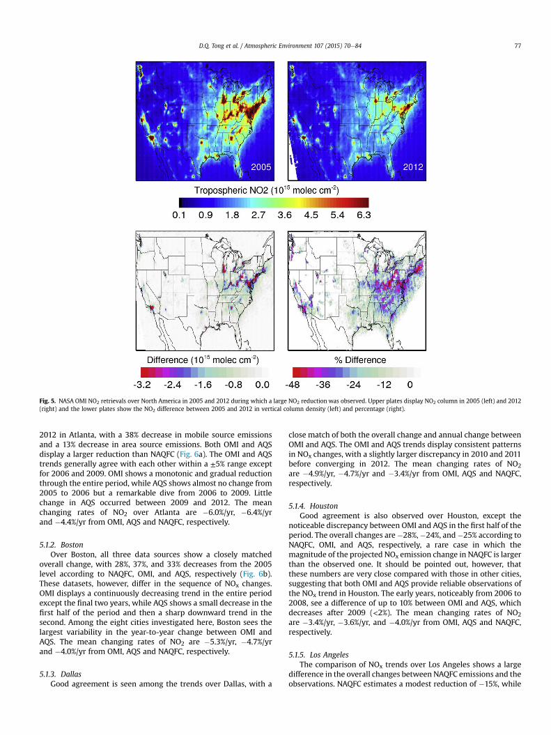
Fig. 5. NASA OMI NO2 retrievals over North America in 2005 and 2012 during which a large NO2 reduction was observed. Upper plates display NO2 column in 2005 (left) and 2012(right) and the lower plates show the NO2 difference between 2005 and 2012 in vertical column density (left) and percentage (right).

D.Q. Tong et al. / Atmospheric Environment 107 (2015) 70e84 77

2012 in Atlanta, with a 38% decrease in mobile source emissionsand a 13% decrease in area source emissions. Both OMI and AQSdisplay a larger reduction than NAQFC (Fig. 6a). The OMI and AQStrends generally agree with each other within a ±5% range exceptfor 2006 and 2009. OMI shows a monotonic and gradual reductionthrough the entire period, while AQS shows almost no change from2005 to 2006 but a remarkable dive from 2006 to 2009. Littlechange in AQS occurred between 2009 and 2012. The meanchanging rates of NO2 over Atlanta are �6.0%/yr, �6.4%/yrand �4.4%/yr from OMI, AQS and NAQFC, respectively.

5.1.2. BostonOver Boston, all three data sources show a closely matched

overall change, with 28%, 37%, and 33% decreases from the 2005level according to NAQFC, OMI, and AQS, respectively (Fig. 6b).These datasets, however, differ in the sequence of NOx changes.OMI displays a continuously decreasing trend in the entire periodexcept the final two years, while AQS shows a small decrease in thefirst half of the period and then a sharp downward trend in thesecond. Among the eight cities investigated here, Boston sees thelargest variability in the year-to-year change between OMI andAQS. The mean changing rates of NO2 are �5.3%/yr, �4.7%/yrand �4.0%/yr from OMI, AQS and NAQFC, respectively.

5.1.3. DallasGood agreement is seen among the trends over Dallas, with a

close match of both the overall change and annual change betweenOMI and AQS. The OMI and AQS trends display consistent patternsin NOx changes, with a slightly larger discrepancy in 2010 and 2011before converging in 2012. The mean changing rates of NO2are �4.9%/yr, �4.7%/yr and �3.4%/yr from OMI, AQS and NAQFC,respectively.

5.1.4. HoustonGood agreement is also observed over Houston, except the

noticeable discrepancy between OMI and AQS in the first half of theperiod. The overall changes are�28%,�24%, and�25% according toNAQFC, OMI, and AQS, respectively, a rare case in which themagnitude of the projected NOx emission change in NAQFC is largerthan the observed one. It should be pointed out, however, thatthese numbers are very close compared with those in other cities,suggesting that both OMI and AQS provide reliable observations ofthe NOx trend in Houston. The early years, noticeably from 2006 to2008, see a difference of up to 10% between OMI and AQS, whichdecreases after 2009 (<2%). The mean changing rates of NO2are �3.4%/yr, �3.6%/yr, and �4.0%/yr from OMI, AQS and NAQFC,respectively.

5.1.5. Los AngelesThe comparison of NOx trends over Los Angeles shows a large

difference in the overall changes between NAQFC emissions and theobservations. NAQFC estimates a modest reduction of �15%, while

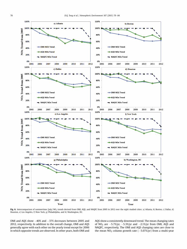
Fig. 6. Intercomparison of summertime (July) NOx trends derived from OMI, AQS, and NAQFC from 2005 to 2012 over the eight studied cities: a) Atlanta, b) Boston, c) Dallas, d)Houston, e) Los Angeles, f) New York, g) Philadelphia, and h) Washington, DC.

D.Q. Tong et al. / Atmospheric Environment 107 (2015) 70e8478

OMI and AQS show �40% and �37% decreases between 2005 and2012, respectively. In addition to the overall change, OMI and AQSgenerally agree with each other on the yearly trend except for 2006inwhich opposite trends are observed. In other years, both OMI and

AQS showa consistently downward trend. Themean changing ratesof NO2 are �5.7%/yr, �5.3%/yr and �2.1%/yr from OMI, AQS andNAQFC, respectively. The OMI and AQS changing rates are close tothe mean NO2 column growth rate (�5.07%/yr) from a multi-year

D.Q. Tong et al. / Atmospheric Environment 107 (2015) 70e84 79

single-sensor analysis based on SCIAMACHY (Schneider and vander A, 2012). A similar changing rate (�5.8%/yr) was also derivedfrom a multi-instrument fitting using the GOME, SCIAMACHY, OMI,and GOME-2 instruments (Hilboll et al., 2013). The large discrep-ancy among the NAQFC, OMI, and AQS trends suggests that theNAQFC emission projection over Los Angeles does not capture themagnitude of recent emission changes.

5.1.6. New YorkBoth OMI and AQS display larger NOx reduction rates than

NAQFC in New York:�32% according to OMI and�45% according toAQS compared with �22% from the data on NAQFC emissions. Themean changing rates of NO2 are �4.6%, �6.4% and �3.1% from OMI,AQS and NAQFC, respectively. The OMI change is smaller than theAQS change in most years, but the two datasets agree well on thedirectionality of the change. Both observations show that thedecrease in NAQFC emissions is insufficient to account for the NOxchange in this area. The annual changing rates from OMI and AQSare comparable to that (�5.3%/yr) derived from SCIAMACHY(Schneider and van der A, 2012), but significantly higher than that(�2.6%/yr) derived from a multi-instrument fitting (Hilboll et al.,2013).

5.1.7. PhiladelphiaThe NAQFC projection (�25%) is comparable to the observed

decrease presented by OMI (�26%), but considerably smaller thanthat by AQS (�37%). Regardless of the large difference in the overallchange, OMI and AQS agree well on the yearly trend across theperiod. The mean changing rates of NO2 are �3.7%/yr, �5.3%/yrand �3.6%/yr from OMI, AQS and NAQFC, respectively.

5.1.8. Washington, DCThe overall change predicted by NAQFC is significantly smaller

than the observations from both OMI and AQS. NAQFC estimatesthat emissions decrease by �28%, while OMI and AQS show �47%and �48% reductions during the same period. The yearly trendsfrom OMI and AQS are also closely matched, in particular in thesecond half of the study period. The mean changing rates of NO2

are �6.7%, �6.9% and �4.0% from OMI, AQS, and NAQFC, respec-tively. Different from trends in other cities, the AQS trend inWashington, DC displays a large reduction in the pre-recessionperiod, and this decrease is even larger than the reduction duringthe recession. Further analysis of the AQS data shows that the pre-recession dive is caused by substantial changes at high NOx sitesfrom 2005 to 2007, which outweighs the changes from other siteswith either lower NOx levels or smaller changes (see Figure S5 inSupplemental Materials). In addition, there are variations in thedata samples used to calculate the trend from AQS (Table 3).

5.2. Comparison of end-of-period change

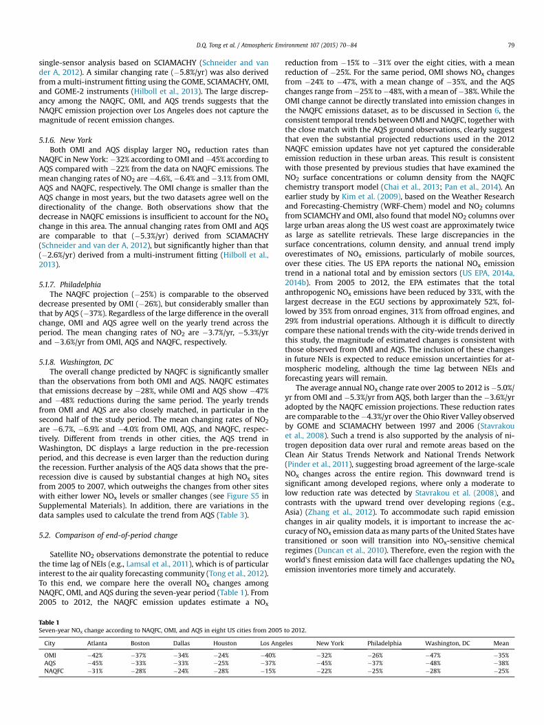
Satellite NO2 observations demonstrate the potential to reducethe time lag of NEIs (e.g., Lamsal et al., 2011), which is of particularinterest to the air quality forecasting community (Tong et al., 2012).To this end, we compare here the overall NOx changes amongNAQFC, OMI, and AQS during the seven-year period (Table 1). From2005 to 2012, the NAQFC emission updates estimate a NOx

Table 1Seven-year NOx change according to NAQFC, OMI, and AQS in eight US cities from 2005

City Atlanta Boston Dallas Houston Los Ange

OMI �42% �37% �34% �24% �40%AQS �45% �33% �33% �25% �37%NAQFC �31% �28% �24% �28% �15%

reduction from �15% to �31% over the eight cities, with a meanreduction of �25%. For the same period, OMI shows NOx changesfrom �24% to �47%, with a mean change of �35%, and the AQSchanges range from�25% to�48%, with a mean of�38%.While theOMI change cannot be directly translated into emission changes inthe NAQFC emissions dataset, as to be discussed in Section 6, theconsistent temporal trends between OMI and NAQFC, together withthe close match with the AQS ground observations, clearly suggestthat even the substantial projected reductions used in the 2012NAQFC emission updates have not yet captured the considerableemission reduction in these urban areas. This result is consistentwith those presented by previous studies that have examined theNO2 surface concentrations or column density from the NAQFCchemistry transport model (Chai et al., 2013; Pan et al., 2014). Anearlier study by Kim et al. (2009), based on the Weather Researchand Forecasting-Chemistry (WRF-Chem) model and NO2 columnsfrom SCIAMCHYand OMI, also found that model NO2 columns overlarge urban areas along the US west coast are approximately twiceas large as satellite retrievals. These large discrepancies in thesurface concentrations, column density, and annual trend implyoverestimates of NOx emissions, particularly of mobile sources,over these cities. The US EPA reports the national NOx emissiontrend in a national total and by emission sectors (US EPA, 2014a,2014b). From 2005 to 2012, the EPA estimates that the totalanthropogenic NOx emissions have been reduced by 33%, with thelargest decrease in the EGU sections by approximately 52%, fol-lowed by 35% from onroad engines, 31% from offroad engines, and29% from industrial operations. Although it is difficult to directlycompare these national trends with the city-wide trends derived inthis study, the magnitude of estimated changes is consistent withthose observed from OMI and AQS. The inclusion of these changesin future NEIs is expected to reduce emission uncertainties for at-mospheric modeling, although the time lag between NEIs andforecasting years will remain.

The average annual NOx change rate over 2005 to 2012 is�5.0%/yr from OMI and �5.3%/yr from AQS, both larger than the �3.6%/yradopted by the NAQFC emission projections. These reduction ratesare comparable to the�4.3%/yr over the Ohio River Valley observedby GOME and SCIAMACHY between 1997 and 2006 (Stavrakouet al., 2008). Such a trend is also supported by the analysis of ni-trogen deposition data over rural and remote areas based on theClean Air Status Trends Network and National Trends Network(Pinder et al., 2011), suggesting broad agreement of the large-scaleNOx changes across the entire region. This downward trend issignificant among developed regions, where only a moderate tolow reduction rate was detected by Stavrakou et al. (2008), andcontrasts with the upward trend over developing regions (e.g.,Asia) (Zhang et al., 2012). To accommodate such rapid emissionchanges in air quality models, it is important to increase the ac-curacy of NOx emission data as many parts of the United States havetransitioned or soon will transition into NOx-sensitive chemicalregimes (Duncan et al., 2010). Therefore, even the region with theworld's finest emission data will face challenges updating the NOxemission inventories more timely and accurately.

to 2012.

les New York Philadelphia Washington, DC Mean

�32% �26% �47% �35%�45% �37% �48% �38%�22% �25% �28% �25%

Table 2Comparisons of NOx changes (%/yr) before, during, and after the 2008 economic recession in the eight urban centers as shown by OMI and AQS.

Stage Sources Atlanta Boston Dallas Houston Los Angeles New York Philadelphia Washington, DC Mean

Before OMI SP �11.7 �9.4 �7.5 �5.7 �3.3 �7.5 �0.6 �12.3 �7.3OMI BEHR �10.1 �14.7 �5.9 �7.6 �5.5 �9.3 �9.4 �9.0 �8.9AQS �9.9 �2.1 �5.2 0.7 �2.0 �5.5 �5.5 �18.7 �6.0

During OMI SP �5.5 �7.5 �8.9 �7.9 �13.1 �6.2 �11.7 �13.0 �9.2OMI BEHR �13.5 0.3 �6.9 �7.7 �15.0 �10.5 �9.9 �9.9 �9.1AQS �17.5 �7.0 �13.0 �14.0 �10.3 �13.6 �7.0 �3.7 �10.8

After OMI SP �6.0 �3.3 �2.1 0.4 �5.0 �3.2 �1.2 �2.3 �2.8OMI BEHR 4.1 �5.5 �1.7 0.3 �2.2 �9.2 �9.3 �5.6 �3.6AQS 1.4 �6.1 0.1 0.2 �6.4 �5.4 �6.1 �5.3 �3.4

Table 3Data points of the NO2 column density from OMI and NOx concentrations from AQS during July from 2005 to 2012.

Year City

Atlanta Boston Dallas Houston Los Angeles New York Philadelphia Washington

OMI AQS OMI AQS OMI AQS OMI AQS OMI AQS OMI AQS OMI AQS OMI AQS

2005 334 561 324 968 415 1403 362 1611 1479 1815 1263 762 332 498 327 4262006 458 580 326 833 475 1232 293 1707 1467 1987 1462 669 354 580 428 3942007 358 452 410 669 437 1233 35 1821 1775 1993 1299 530 337 441 321 8722008 532 437 378 868 526 1276 443 1730 1590 1946 1419 687 353 458 341 7192009 440 356 295 694 364 1225 441 1747 1460 1983 1332 682 376 237 370 7822010 486 342 264 852 366 1524 259 1704 1458 1871 1659 566 463 336 438 7912011 520 342 339 928 575 1604 470 1831 1459 1859 1605 326 380 357 347 6882012 545 343 393 923 500 1155 284 1855 840 1680 1464 471 393 473 312 796

D.Q. Tong et al. / Atmospheric Environment 107 (2015) 70e8480

5.3. Impact of economic recession on NOx emissions

In all cities examined in this study, we found that the first half ofthe period sees a greater NOx reduction than the second half,perhaps because of the combined effects of emission control reg-ulations and economic recession. In recent decades, regional andnational emission control programs, such as the Ozone TransportRegion (OTR) NOx Cap and Allowance Trading Program, the NOxState Implementation Plan (SIP) Call, and the Cross-State AirPollution Rule (CSAPR), have been implemented that aim to reduceanthropogenic NOx emissions frommajor sources in North America(Richter et al., 2005; Kim et al., 2009; Stavrakou et al., 2008; van derA et al., 2008; Konovalov et al., 2010; Russell et al., 2010). Similartrends have also been observed in other developed regionsincluding Europe and Japan (van der A et al., 2008; Konovalov et al.,2010; Castellanos and Boersma, 2012). Meanwhile, economicdevelopment and increases in energy use have been associatedwith the observed rises in NOx emissions over developing countries(van der A et al., 2008; Zhou et al., 2012). The impact of the 2008global economic recession on US NOx emissions was examined byRussell et al. (2012) using OMI Berkeley High Resolution (BEHR)product. They found that the decreases in urban NO2 columndensities accelerated during the recession, changing from �6%/yrbeforehand to �8%/yr during the financial crisis, and then slowingto �3%/yr thereafter (Russell et al., 2012). Satellite and groundobservations were also used to quantify the impact of the economicrecession on air quality in Greece (Vrekoussis et al., 2013) andpollution emissions from marine shipping lanes (de Ruyter deWildt et al., 2012). Collectively, these studies demonstrate that itis possible to use satellite observations to detect the effect of short-term economic fluctuations on NOx emissions.

Following the definition of Russell et al. (2012), we divide theseven-year study period into three stages in order to examine theNOx rates of change before (2005e2007), during (2008e2009), andafter (2010e2012) the economic recession. Table 2 shows the yearlyNOx rates of change for each subperiod. In addition to the OMIStandard Product (OMI SP) and AQS data used here, we also include

in Table 2 the results extracted from OMI BEHR (Russell et al., 2012)for comparison purposes. Table 2 shows considerable variability inthe magnitude of NOx changes from city to city. The AQS dataclearly display larger reduction rates during the recession thanbefore the recession in all cities except Washington DC. The OMIdata also show larger reduction during the recession in five of theeight cities, but the reduction rate is generally smaller than thatfrom the AQS data. In the other three cities (Atlanta, Boston, andNew York), the reduction rate fromOMIwas actually smaller duringrecession than before recession, different from that by AQS. Bycomparison the rates of change derived from the OMI BEHR dataare different from those derived from OMI SP. The difference in theNO2 trends between the two OMI products is attributed to severalfactors, including retrieval approaches, data filtering criteria, andspatial and temporal coverage. In particular, Russell et al. (2012)derived the BEHR OMI trends using 12-month data, while thisstudy is limited to the July data. The temporal coverage affects notonly the size of data samples, but also other relevant factors such asthe relative contribution of local emissions and regional transportto NO2 columns since the lifetime of NO2 is shorter in July than incold seasons. In summary, there are inconsistencies in the detailedtrends before, during and after recession at the city level. Futurework is needed to extend this study beyond July to examine if suchresponse to economic recession also exists in other months. Whilethe OMI SP data are used here to exemplify the feasibility of usingsatellite data to validate emission updates, other NO2 products(such as BEHR, DOMINO and GOME2) should be considered in thefuture to obtain a broader view of the emission trends.

6. Discussion of uncertainties

There are several factors contributing to the uncertainties in thethree-member intercomparisons presented in Fig. 6. These factorsinclude data quality in AQS and OMI data, uncertainties in NOxemission model data, representativeness of NOx life cycles bydifferent datasets, and mismatched sampling time between OMIand AQS. We discuss below how these factors may affect the

D.Q. Tong et al. / Atmospheric Environment 107 (2015) 70e84 81

interpretation of the trend comparison. The trend data derivedfrom both OMI and AQS have gone through rigorous qualityfiltering as described Sections 2.3. However, the quality filteringprocedures also affect the completeness of individual dataset. ForOMI, the criteria applied to screen NO2 data by cloudiness and rowanomaly flag will reduce the size of data samples, resulting invarying data points eventually used to represent the OMI trend.Similarly, instrumental malfunctioning and other errors could leadto loss of valid data points from the AQS network. Table 3 lists thenumbers of OMI and AQS data points used to derive the NOx trendsin each city. There are noticeable variations in the number of datapoints from both datasets. For instance, over Atlanta, there arefewer valid data points from OMI, but more from AQS during2005e2007. The change in data samples is likely a cause of thediscrepancy between the OMI and AQS trends in Fig. 6a. There are alarge number of data points excluded (due to clouds) from OMI in2006 and 2007 over Houston, which could be responsible for thedifference between the OMI trend and that from AQS and NAQFC(Fig. 6d). There are a smaller number of AQS observations in 2005and 2006 over Washington, DC. that likely contributes to the largedecrease between 2005 and 2008 over this area (Fig. 6f). Regardlessof the large variations in data samples, both datasets revealconsistent downward NOx trends, suggesting a certain level ofrepresentativeness of the validated data samples, although it isdifficult to quantitatively assess the uncertainties caused by themissing data.

The NOx trends examined here were obtained from three datasources that represent different aspects of the NOx life cycle. OMIobserves NO2 column density in the troposphere, AQS monitorsNOx concentrations at the surface, and NEI describes the verticalflux rate immediately after being released into the atmosphere.Complicated processes including chemical transformation, trans-port, and deposition alter the relationships among these NOx var-iables, making the direct comparison of their values extremelychallenging. Our approach in this study compares the interannualtrends derived from individual datasets, thereby minimizing theinterference of certain factors affecting the relationships amongthem. Even so, some remaining issues must be recognized wheninterpreting our results, including the varying relationships amongNOx emissions, surface concentration, the atmospheric column, andthe mismatched “sampling” time.

One of the concerns about the intercomparison is that therelationship between NO2 column and NOx emissions varies overspace and time, making it challenging directly comparing the twoparameters (Lamsal et al., 2011). Most urban centers examined inthis study are in NOx-saturated chemical regimes (e.g., Tong et al.,2006; Duncan et al., 2010). Enhanced near-source deposition andchemical destruction occur when dense NOx emissions areconfined in urban plumes, where the limited availability of andmixing with volatile organic compounds constrains the preserva-tion of emitted NOx in the atmosphere (Ryerson et al., 1998). As NOxemissions decrease over time, the chemical regime and near-sourceremoval change, and this change subsequently affects the re-lationships among emissions, ambient concentration, and verticalcolumn through a chain of chemical and photochemical reactions(Warneck, 2000). One of these relationships is the local sensitivityof NO2 column change to changes in NOx emissions, represented byb in the following equation (Lamsal et al., 2011):

DE=E ¼ b� DU=U (2)

where DU is the column change driven by the change in emissionsDE. In order to directly compare the trends from OMI and NAQFC orother emission inventories, it is necessary to assume that thechange in b over one metropolitan area is small enough for this

factor to be canceled out when deriving the long-term trend. Theoverall difference in these trends is a combination of the changes inNOx emissions, columns, and their relative sensitivity. For example,by using the global chemical transport model GEOS-Chem, Lamsalet al. (2011) found that a perturbation of 30% only changes b by<2%.Therefore, the overall error caused by non-uniformity of b is ex-pected to be small compared with the NOx trends, since the annualNOx change over a city is relatively small (�5%) and the seven-yearchanges are approximately 30% in most cases (Table 1). Our ownsimulations with the NAQFC CMAQ model showed a similarmagnitude of sensitivities between NOx emissions and the NO2column.

Another concern about the intercomparison is that differentsampling times were used for different datasets. The NAQFCemission model uses a diurnal profile to split total NOx emissionsinto hourly data, meaning that sampling time does not alter therelative change or trend. There is, however, a mismatch in thetemporal resolutions between AQS and OMI. AQS samples NOxconcentrations hourly, while OMI observes the NO2 column onlyonce a day. In this study, we used early morning rush-hour data toderive the NOx trend fromNAQFC and AQS, but early afternoon datafor the OMI trend. It thus remains unclear if the difference insampling time affects the derived NOx trends. To examine thisissue, we repeated the AQS data analysis, but by using the earlyafternoon hours covering the OMI passing time (12e3 pm localtime). We then compared the annual trends in AQS in both earlymorning and early afternoonwith the OMI data in order to examinethe difference between the two AQS datasets as well as betweenthe AQS and OMI observations (Fig. 7). Compared with the earlymorning data, the afternoon AQS data display larger year-to-yearvariability, particularly over Atlanta, Boston, and Dallas. In othercities, the difference is smaller. For all cities, there is a consistentdownward trend during this period, and the trend is generally inaccord with the OMI trend. Between the morning and afternoonAQS trends, the former is better correlated with the OMI trend,perhaps because of the stronger dominance of local emissions andweaker interference of meteorology and photochemistry in earlymorning and the locality of surface sites (Steinbacher et al., 2007).This is consistent with an earlier NOx budget study using amodeling technique called budget process analysis (Tong et al.,2005) which shows that NOx budget is largely controlled bychemistry and transport even in rural area where emissions andchemical processes are less vibrant as in urban areas. The betteragreement between OMI and early morning AQS data, however,does not necessarily imply that early morning is an ideal timewindow for space-based observations, since surface concentrationand column density display distinct responsiveness to the chemicaland physical processes affecting the NOx life cycle. Unfortunatelyreliable fine-resolution satellite and ground NO2 data are notavailable, which limits comparison of NOx trends from differentobservations.

7. Conclusion and recommendations

This study derives multi-year NOx trends from satellite andground observations and uses these data to evaluate the emissionupdates for the US NAQFC predictions. Over the eight US citiesexamined here, both OMI and AQS show substantial downwardtrends from 2005 to 2012. The NOx emission projection adopted byNAQFC tends to be in the right direction with the observed NOx

trend, but at a slower reduction rate (�25% in seven years vs.about �35% from OMI -38% from AQS), perhaps because of unac-counted effects of the 2008 economic recession in the NAQFCemissions. Both OMI and AQS datasets display distinct emissionreduction rates before, during, and after the 2008 global recession

Fig. 7. Comparison of OMI NO2 trend with NOx trends derived from AQS during early morning (6e9 am local time) and early afternoon (12e3 pm) from 2005 to 2012 over eightcities: a) Atlanta, b) Boston, c) Dallas, d) Houston, e) Los Angeles, f) New York, g) Philadelphia, and h) Washington, DC.

D.Q. Tong et al. / Atmospheric Environment 107 (2015) 70e8482

in several cities, but the detailed changing rates are not necessarilyconsistent between the OMI and AQS data. NAQFC predictions ofsurface ozone concentrations were shown to have improvedfollowing the update for NOx emissions in year 2012.

This study demonstrates the feasibility of using space andground observations to objectively evaluate major updates ofemission inventories, which are crucial to predict air quality accu-rately. It is interesting to note that the OMI-based NO2 trend closely

D.Q. Tong et al. / Atmospheric Environment 107 (2015) 70e84 83

matches the AQS ground observations of not only the overallreduction, but also the gradual series of NOx changes. Given thewide spatial coverage and near real-time data availability, satelliteNO2 observations thus show a great potential to improve thequality of NOx emission inventories used by time-sensitive appli-cations, as suggested in earlier studies (Lamsal et al., 2011; Tonget al., 2012; Streets et al., 2013). Ground NOx observations, partic-ularly the morning rush-hour data, are another valuable datasource that can be used in order to evaluate and improve emissioninventories, although the monitors are mostly confined in urbanareas. The combination of satellite, ground observations, and in-situ measurements (e.g., the CEM data in Frost et al., 2006) islikely to provide more reliable estimates of NOx emissions and theirtrends, which is an issue of increasing importance as many urbanareas in the US are transitioning to NOx-sensitive chemical regimeswith continuous emission reductions. It is also desirable to developan emission data assimilation capability that allows timely inges-tion of these observational data in order to address major emissionuncertainties (e.g., Tong et al., 2012) in time-sensitive applicationssuch as air quality forecasting.

Acknowledgments

This work has been supported by the NOAA JPSS Proving Groundand Risk Reduction Program (NA12NES4400007) and the NASAEarth Science Program through the National Climate Indicator(NNX13A045G) and Air Quality Applied Science Team initiatives.The authors are grateful to Dr. Bryan Duncan at NASA and twoanonymous reviewers for their constructive comments.

Appendix A. Supplementary data

Supplementary data related to this article can be found at http://dx.doi.org/10.1016/j.atmosenv.2015.01.035.

References

Boersma, K.F., Eskes, H.J., Brinksma, E.J., 2004. Error analysis for tropospheric NO2retrieval from space. J. Geophys. Res. 109, D04311. http://dx.doi.org/10.1029/2003JD003962.

Boersma, K.F., Eskes, H.J., Veefkind, J.P., Brinksma, E.J., van der A, R.J., Sneep, M., vanden Oord, G.H.J., Levelt, P.F., Stammes, P., Gleason, J.F., Bucsela, E.J., 2007. Near-real time retrieval of tropospheric NO2 from OMI. Atmos. Chem. Phys. 7,2103e2118. http://dx.doi.org/10.5194/acp-7-2103-2007.

Bond, T.C., Streets, D.G., Yarber, K.F., Nelson, S.M., Woo, J.-H., Klimont, Z., 2004.A technology-based global inventory of black and organic carbon emissionsfrom combustion. J. Geophys. Res. 109, D14203. http://dx.doi.org/10.1029/2003JD003697.

Bucsela, E.J., Krotkov, N.A., Celarier, E.A., Lamsal, L.N., Swartz, W.H., Bhartia, P.K.,Boersma, K.F., Veefkind, J.P., Gleason, J.F., Pickering, K.E., 2013. A new strato-spheric and tropospheric NO2 retrieval algorithm for nadir-viewing satelliteinstruments: application to OMI. Atmos. Meas. Tech. 6, 2607e2626.

Byun, D., Schere, K.L., 2006. Review of the governing equations, computational al-gorithms, and other components of the models-3 community multiscale airquality (CMAQ) modeling system. Appl. Mech. Rev. 55, 51e77.

Castellanos, P., Boersma, K.F., 2012. Reductions in nitrogen oxides over Europedriven by environmental policy and economic recession. Sci. Reports 2 (265),1e7. http://dx.doi.org/10.1038/srep00265.

Chai, T., Kim, H.-C., Lee, P., Tong, D., Pan, L., Tang, Y., Huang, J., McQueen, J.,Tsidulko, M., Stajner, I., 2013. Evaluation of the United States National AirQuality Forecast Capability experimental real-time predictions in 2010 using AirQuality System ozone and NO2 measurements. Geosci. Model Dev. 6,1831e1850. http://dx.doi.org/10.5194/gmd-6-1831-2013.

Choi, Y., Kim, H., Tong, D., Lee, P., 2012. Summertime weekly cycles of observed andmodeled NOx and O3 concentrations as a function of satellite-derived ozoneproduction sensitivity and land use types over the Continental United States.Atmos. Chem. Phys. 12, 6291e6307. http://dx.doi.org/10.5194/acp-12-6291-2012.

Crutzen, P.J., Gidel, L.T., 1983. A two-dimensional photochemical model of the at-mosphere, 2, the tropospheric budgets of the anthropogenic chlorocarbons CO,CH4, CH3C1 and the effect of various NOx sources on tropospheric ozone.J. Geophys. Res. 88, 6641e6661.

de Ruyter de Wildt, M., Eskes, H., Boersma, K.F., 2012. The global economic cycle and

satellite-derived NO2 trends over shipping lanes. Geophys. Res. Lett. 39, L01802.http://dx.doi.org/10.1029/2011GL049541.

Dobber, M.R., Braak, R., 2010. Known Instrumental Affects that Affect the OMI L1BProduct of the Ozone Monitoring Instrument on EOS Aura. Last update: 17December 2010. http://disc.sci.gsfc.nasa.gov/Aura/data-holdings/OMI/documents/v003/known_instrumental_effects_l1b_data_omi_v6.pdf.

Duncan, B., Yoshida, Y., Olson, J., Sillman, S., Retscher, C., Martin, R., Lamsal, L., Hu, Y.,Pickering, K., Retscher, C., Allen, D., Crawford, J., 2010. Application of OMI ob-servations to a space-based indicator of NOx and VOC controls on surface ozoneformation. Atmos. Environ. 44, 2213e2223. http://dx.doi.org/10.1016/j.atmosenv.2010.03.010.

Duncan, B., Yoshida, Y., de Foy, B., Lamsal, L., Streets, D., Lu, Z., Pickering, K.,Krotkov, N., 2013. The observed response of Ozone Monitoring Instrument(OMI) NO2 columns to NOx emission controls on power plants in the UnitedStates: 2005-2011. Atmos. Environ. 81, 102e111. http://dx.doi.org/10.1016/jatmosenv.2013.08.068.

Dunlea, E.J., Herndon, S.C., Nelson, D.D., Volkamer, R.M., San Martini, F.,Sheehy, P.M., Zahniser, M.S., Shorter, J.H., Wormhoudt, J.C., Lamb, B.K.,Allwine, E.J., Gaffney, J.S., Marley, N.A., Grutter, M., Marquez, C., Blanco, S.,Cardenas, B., Retama, A., Ramos Villegas, C.R., Kolb, C.E., Molina, L.T.,Molina, M.J., 2007. Evaluation of nitrogen dioxide chemiluminescence monitorsin a polluted urban environment. Atmos. Chem. Phys. 7, 2691e2704. http://dx.doi.org/10.5194/acp-7-2691-2007.

Eder, B., Kang, D., Mathur, R., Pleim, J., Yu, S., Otte, T., Pouliot, G., 2009.A performance evaluation of the National Air Quality Forecast Capability for thesummer of 2007. Atmos. Environ. 43, 2312e2320.

Frost, G.J., et al., 2006. Effects of changing power plant NOx emissions on ozone inthe eastern United States: proof of concept. J. Geophys. Res. 111, D12306. http://dx.doi.org/10.1029/2005JD006354.

Godowitch, J.M., Pouliot, G., Rao, S.T., 2010. Assessing multi-year changes inmodeled and observed urban NOx concentrations from a dynamic modelevaluation perspective. Atmos. Environ. 44 (24), 2894e2901.

Granier, C., et al., 2011. Evolution of anthropogenic and biomass burning emissionsof air pollutants at global and regional scales during the 1980e2010 period.Clim. Change 109, 163e190.

Harley, R.A., Marr, L.C., Lehner, J.K., Giddings, S.N., 2005. Changes in motor vehicleemissions on diurnal to decadal time scales and effects on atmosphericcomposition. Environ. Sci. Tech. 39, 5356e5362.

Hilboll, A., Richter, A., Burrows, J.P., 2013. Long-term changes of tropospheric NO2over megacities derived from multiple satellite instruments. Atmos. Chem.Phys. 13, 4145e4169.

Houyoux, M.R., Vukovich, J.M., Coats Jr., C.J., Wheeler, N.J.M., Kasibhatla, P.S., 2000.Emission inventory development and processing for the seasonal model forRegional Air Quality (SMRAQ) Project. J. Geophys. Res. 105 (D7), 9079e9090.

Hudman, R.C., Moore, N.E., Mebust, A.K., Martin, R.V., Russell, A.R., Valin, L.C.,Cohen, R.C., 2012. Steps towards a mechanistic model of global soil nitric oxideemissions: implementation and space based-constraints. Atmos. Chem. Phys.12, 7779e7795. http://dx.doi.org/10.5194/acp-12-7779-2012.

Jerrett, M., Burnett, R.T., Pope III, C.A., Ito, K., Thurston, G., Krewski, D., et al., 2009.Long-term ozone exposure and mortality. N. Engl. J. Med. 360, 1085e1095.

Kang, D., Mathur, R., Rao, S.T., 2010. Real-time bias-adjusted O3 and PM2.5 air qualityindex forecasts and their performance evaluations over the continental UnitedStates. Atmos. Environ. 44, 2203e2212.

Kim, S.W., Heckel, A., Frost, G.J., Richter, A., Gleason, J., Burrows, J.P., McKeen, S.,Hsie, E.Y., Granier, C., Trainer, M., 2009. NO2 columns in the western UnitedStates observed from space and simulated by a regional chemistry model andtheir implications for NOx emissions. J. Geophys. Res. 114, D11301. http://dx.doi.org/10.1029/2008JD011343.

Konovalov, I.B., Beekmann, M., Richter, A., Burrows, J.P., Hilboll, A., 2010. Multi-annual changes of NOx emissions in megacity regions: nonlinear trend analysisof satellite measurement based estimates. Atmos. Chem. Phys. 10, 8481e8498.http://dx.doi.org/10.5194/acp-10-8481-2010.

Lamsal, L.N., Martin, R.V., Padmanabhan, A., van Donkelaar, A., Zhang, Q., Sioris, C.E.,Chance, K., Kurosu, T.P., Newchurch, M.J., 2011. Application of satellite obser-vations for timely updates to global anthropogenic NOx emission inventories.Geophys. Res. Lett. 38, L05810. http://dx.doi.org/10.1029/2010GL046476.

Lamsal, Lok N., Duncan, Bryan N., Yoshida, Yosuko, Krotkov, Nickolay A.,Pickering, Kenneth E., Streets, David G., Lu, Zifeng, 2015. U.S. NO2 trends(2005e2013): EPA Air Quality System (AQS) data versus improved observationsfrom the Ozone Monitoring Instrument (OMI). Atmos. Environ (submitted forpublication).

Lee, P., Fong, N., 2011. Coupling of important physical processes in the planetaryboundary layer between meteorological and chemistry models for regional toContinental scale air quality forecasting: an overview. Atmosphere 2 (3),464e483.

Levelt, P.F., van den Oord, G.H.J., Dobber, M.R., M€alkki, A., Visser, H., de Vries, J.,Stammes, P., Lundell, J.O.V., Saari, H., 2006. The ozone monitoring instrument.IEEE Trans. Geosci. Remote Sens. 44, 1093e1101. http://dx.doi.org/10.1109/TGRS.2006.872333.

Liu, S.C., Trainer, M., Fehsenfeld, F., Parrish, D.D., Williams, E.J., Fahey, D.W.,Htibler, G., Murphy, P.C., 1987. Ozone production in the rural troposphere andthe implications for regional and global ozone distributions. J. Geophys. Res. 92,4191e4207.

Martin, R.V., et al., 2002. An improved retrieval of tropospheric nitrogen dioxidefrom GOME. J. Geophys. Res. 107 (D20), 4437. http://dx.doi.org/10.1029/

D.Q. Tong et al. / Atmospheric Environment 107 (2015) 70e8484

2001JD001027.Martin, R.V., Jacob, D.J., Chance, K., Kurosu, T.P., Palmer, P.I., Evans, M.J., 2003. Global

inventory of nitrogen oxide emissions constrained by space-based observationsof NO2 columns. J. Geophys. Res. 108 (D17), 4537. http://dx.doi.org/10.1029/2003JD003453.

McClenny, W.A., Williams, E.J., Cohen, R.C., Stutz, J., 2002. Preparing to measure theeffects of the NOx SIP call e methods for ambient air monitoring of NO, NO2,NOy, and individual NOz species. J. Air Waste Manage. Assoc. 52, 542e562.

Mijling, B., van derA, R.J., 2012. Using daily satellite observations to estimateemissions of short-lived air pollutants on a mesoscopic scale. J. Geophys. Res.117, D17302. http://dx.doi.org/10.1029/2012JD017817.

Oetjen, H., Baidar, S., Krotkov, N.A., Lamsal, L.N., Lechner, M., Volkamer, R., 2013.Airborne MAX-DOAS measurements over California: testing the NASA OMItropospheric NO2 product. J. Geophys. Res. 118, 13. http://dx.doi.org/10.1002/jdrd.50550.

Otte, T.L., et al., 2005. Linking the Eta model with the Community Multiscale AirQuality (CMAQ) modeling system to build a national air quality forecastingsystem. Weather Forecast. 20, 367e384.

Pan, L., Tong, D.Q., Lee, P., Kim, H., Chai, T., 2014. Assessment of NOx and O3 fore-casting performances in the U.S. National Air Quality Forecasting Capabilitybefore and after the 2012 major emissions updates. Atmos. Environ. 95,610e619.

Pinder, R.W., Appel, K.W., Dennis, R.L., 2011. Trends in atmospheric reactive nitrogenfor the Eastern United States. Environ. Pollut. 159, 3138e3141.

Platt, U., 1994. Differential optical absorption spectroscopy (DOAS). Chem. Anal. Ser.127, 27e83.

Pope III, C.A., Burnett, R.T., Thun, M.J., Calle, E.E., Krewski, D., Ito, K., Thurston, G.D.,2002. Lung cancer, cardiopulmonary mortality, and long-term exposure to fineparticulate air pollution. J. Am. Med. Assoc. 12, 1132e1141. http://dx.doi.org/10.1001/jama.287.9.1132.

Richter, A., Burrows, J.P., Nüb, H., Granier, C., Niemeier, U., 2005. Increase intropospheric nitrogen oxide over China observed from space. Nat. Lett. 437,129e132. http://dx.doi.org/10.1038/nature04092.

Russell, A.R., Valin, L.C., Buscela, E.J., Wenig, M.O., Cohen, R.C., 2010. Space-basedconstraints on spatial and temporal patterns in NOx emissions in California,2005e2008. Environ. Sci. Technol. 44, 3607e3615.

Russell, A.R., Valin, L.C., Cohen, R.C., 2012. Trends in OMI NO2 observations over theUnited States: effects of emission control technology and the economic reces-sion. Atmos. Chem. Phys. 12, 12197e122209. http://dx.doi.org/10.5194/acp-12-12197-2012.

Ryerson, T.B., et al., 1998. Emissions lifetimes and ozone formation in power plantplumes. J. Geophys. Res. 103 (D17), 22569e22583. http://dx.doi.org/10.1029/98JD01620.

Schneider, P., van der A, R.J., 2012. A global single-sensor analysis of 2002e2011tropospheric nitrogen dioxides trends observed from space. J. Geophys. Res. 117,D16309. http://dx.doi.org/10.1029/2012JD017571.

Spicer, C.W., 1983. Smog chamber studies of NOx transformation rate and nitrate/precursor relationships. Environ. Sci. Technol. 17, 112e120.

Stajner, I., Davidson, P., Byun, D., McQueen, J., Draxler, R., Dickerson, P., Meagher, J.,2012. US national air quality forecast capability: expanding coverage to includeparticulate matter. In: Steyn, Douw G., Castelli, Silvia Trini (Eds.), NATO/ITM AirPollution Modeling and its Application, vol. XXI. Springer, Netherlands,pp. 379e384. http://dx.doi.org/10.1007/978-94-007-1359-8_64.

Stavrakou, T., Muller, J.F., Boersma, K.F., De Smedt, I., van der A, R.J., 2008. Assessingthe distribution and growth rates of NOx emission sources by inverting a 10-

year record of NO2 satellite columns. Geophys. Res. Lett. 35, L10801. http://dx.doi.org/10.1029/2008GL033521.

Steinbacher, M., Zellweger, C., Schwarzenbach, B., Bugmann, S., Buchmann, B.,Ord�o~nez, C., Prevot, A.S.H., Hueglin, C., 2007. Nitrogen oxides measurements atrural sites in Switzerland: bias of conventional measurement techniques. J.Geophys. Res. D11307. http://dx.doi.org/10.1029/2006JD007971.

Streets, D.G., et al., 2013. Emissions estimation from satellite retrievals: a review ofcurrent capability. Atmos. Environ. 77, 1011e1042.

Tong, D.Q., Mauzerall, D.L., 2006. Spatial variability of summertime tropospheric O3in the continental United States: an evaluation of the CMAQ model and itsimplications. Atmos. Environ. 40, 3041.

Tong, D.Q., Kang, D., Viney, P.A., Rayb, J.D., 2005. Reactive Nitrogen Oxides in theSoutheast United States National Parks: Source Identification.

Tong, D.Q., Muller, N., Mauzerall, D.L., Mendelsohn, R., 2006. An integratedassessment of the impacts of ozone resulting from nitrogen oxide emissionsnear Atlanta. Environ. Sci. Technol. 40 (5), 1395.

Tong, D.Q., Mathur, R., Schere, K., Kang, D., Yu, S., 2007. The use of air qualityforecasts to assess impacts of air pollution on crops: a case study of assessingsoybean yield losses from ozone in the United States. Atmos. Environ. 41 (38),8772e8784.

Tong, D.Q., Mathur, R., Kang, D., Yu, S., Schere, K.L., Pouliot, G., 2009. Vegetationexposure to ozone over the continental United States: assessment of exposureindices by the Eta-CMAQ air quality forecast model. Atmos. Environ. 43 (3),724e733.

Tong, D.Q., Lee, P., Saylor, R.D., 2012. New Direction: the need to develop process-based emission forecasting models. Atmos. Environ. 47, 560e561.

US DOE, 2012. Annual Energy Outlook 2012. DOE Energy Information Agency (EIA).Document No. DOE/EIA-0383(2012). Accessed online Nov 18, 2012 at. http://www.eia.gov/forecasts/aeo/pdf/0383(2012).pdf.

US EPA, 2011. Technical Support Document (TSD) for the Final Transport Rule.Docket ID No. EPA-HQ-OAR-2009-0491 (accessed online Nov 18, 2012 at. http://www.epa.gov/airtransport/pdfs/EmissionsInventory.pdf.

US EPA, 2014a. The Green Book Nonattainment Areas for Criteria Pollutants.Available online at: http://www.epa.gov/airquality/greenbook/index.html(accessed on 10.02.14.).

US EPA, 2014b. 1970e2013 Average Annual Emissions, from National Emission In-ventory (NEI) Air Pollutant Trends Data. Available online at: http://www.epa.gov/ttn/chief/trends/trends06/national_tier1_caps.xlsx (accessed on 10.02.14.).

van der A, R.J., Eskes, H.J., Boersma, K.F., van Noije, T.P.C., Van Roozendael, M., DeSmedt, I., Peters, D.H.M.U., Meijer, E.W., 2008. Trends, seasonal variability anddominant NOx source derived from a ten year record of NO2 measured fromspace. J. Geophys. Res. 113, D04302. http://dx.doi.org/10.1029/2007JD009021.

Vrekoussis, M., Richter, A., Hilboll, A., Burrows, J.P., Gerasopoulos, E., Lelieveld, J.,Barrie, L., Zerefos, C., Mihalopoulos, N., 2013. Economic crisis detected fromspace: air quality observations over Athens/Greece. Geophys. Res. Lett. 40,458e463. http://dx.doi.org/10.1002/grl.50118.

Warneck, P., 2000. Chemistry of the Natural Atmosphere, Second ed. AcademicPress, ISBN 0-12-735632-0.

Zhang, Q., Geng, G.N., Wang, S.W., Richter, A., He, K.B., 2012. Satellite remote sensingof changes in NOx emissions over China during 1996e2010, Chinese. Sci. Bull.57, 2857e2864.

Zhou, Y., Brunner, D., Hueglin, C., Henne, S., Staehelin, J., 2012. Changes in OMItropospheric NO2 columns over Europe from 2004 to 2009 and the influence ofmeteorological variability. Atmos. Environ. 46, 482e495.