LONG-TERM COOLING OF AN SBLOCA: BORON PRECIPITATION …€¦ · TM plant, events such as the...
131
LONG-TERM COOLING OF AN SBLOCA: BORON PRECIPITATION IN THE CORE, BORON DILUTION IN THE STEAM GENERATORS Lisa M. Gerken Thesis submitted to the faculty of the Virginia Polytechnic Institute and State University in partial fulfillment of the requirements for the degree of Master of Science In Mechanical Engineering Yang Liu Mark Pierson Liliane Schor December 11, 2013 Blacksburg, VA Keywords: Small break LOCA, boron dilution, boron precipitation, long-term core cooling Copyright 2013
Transcript of LONG-TERM COOLING OF AN SBLOCA: BORON PRECIPITATION …€¦ · TM plant, events such as the...

LONG-TERM COOLING OF AN SBLOCA: BORON PRECIPITATION IN THE CORE,
BORON DILUTION IN THE STEAM GENERATORS
Lisa M. Gerken
Thesis submitted to the faculty of the Virginia Polytechnic Institute and State University in
partial fulfillment of the requirements for the degree of
Master of Science In
Mechanical Engineering
Yang Liu Mark Pierson Liliane Schor
December 11, 2013 Blacksburg, VA
Keywords: Small break LOCA, boron dilution, boron precipitation, long-term core cooling
Copyright 2013

Long-term Cooling of an SBLOCA: Boron Precipitation in the Core, Boron Dilution in the Steam Generators
Lisa M. Gerken
ABSTRACT
When soluble boron is used to control reactivity, there are two particular events which can
challenge long-term core cooling (LTCC) during the small break loss-of-coolant accident (SBLOCA):
boron precipitation and boron dilution. The initial consequences of the SBLOCA are mitigated by the
emergency safety systems, but the core continues to boil. As boron is less volatile than steam, the steam
is virtually boron-free. All the boron remains in the core, the boron concentration in the core rises. If
the solubility limit is reached, precipitation could occur. The boron precipitation event was historically
considered to be bounded by the large break accident. However, there are characteristics of the
SBLOCA which cannot be neglected and an SBLOCA-specific methodology is required. On the
opposite end of the boron concentration spectrum is the SBLOCA boron dilution event. The steam
generators remove heat from the primary and condense the steam. The condensation of the boron-free
steam can result in the accumulation of a deborated slug of water. If natural circulation restarts, the slug
can be transported toward the core and potentially reduce the core boron concentration enough to induce
a recriticality.
This thesis describes two analytical methodologies for these SBLOCA LTCC events. The two
methodologies have a similar approach. Both use transient system analyses for inputs to and
justification of the follow-on boron concentration calculations. For boron precipitation, a maximized
concentration is calculated with the Small Break Boron Precipitation model. For boron dilution, a
minimized core inlet concentration is calculated using computational fluid dynamics.
NOTE: Portions of this thesis have been redacted due to the proprietary nature of the content. The information was provided for the committee’s review. The redaction of the information in this version does not alter the conclusions of the thesis.

iii
TABLE OF CONTENTS Page
ABSTRACT ............................................................................................................................................... ii
LIST OF TABLES ..................................................................................................................................... v
LIST OF FIGURES .................................................................................................................................. vi
TABLE OF ACRONYMS ...................................................................................................................... viii
1.0 INTRODUCTION ........................................................................................................................... 1
1.1 Long-Term Core Cooling of an SBLOCA .......................................................................... 1
1.2 Analytical Methodologies for Long-Term Core Cooling of an SBLOCA .......................... 2
2.0 BORON PRECIPITATION ............................................................................................................ 4
2.1 Historical Background ......................................................................................................... 4
2.2 SBLOCA Boron Precipitation Phenomena ......................................................................... 6
2.3 Boron Precipitation Analytical Methodology ...................................................................... 7
2.4 Development of an SBLOCA Boron Precipitation Analytical Methodology ..................... 9
3.0 SBBP MODEL .............................................................................................................................. 11
3.1 SBBP Model: Concentrating Volume Concentration Analysis ......................................... 12 3.1.1 Pre-Pool-Boiling Concentrating Volume Concentration ..................................... 13
3.1.2 Steaming Rate ...................................................................................................... 13
3.1.3 Injection Rate ....................................................................................................... 15
3.1.4 Injection Boron Concentration ............................................................................. 16
3.1.5 Concentrating Volume Boron Content ................................................................. 17
3.1.6 Concentrating Volume Boron Concentration ....................................................... 17
3.2 SBBP Model: Solubility Limit .......................................................................................... 17
3.3 SBBP Model: Hot Leg Injection Dilution Analysis .......................................................... 22
3.3.1 HLI Boiloff ........................................................................................................... 22
3.3.2 Excess HLI ........................................................................................................... 23
3.3.3 Dilution Concentration ......................................................................................... 23
3.3.4 SBBP Model: Summary of Assumptions and Conservatisms ............................. 24
4.0 DEMONSTRATION OF SBBP MODEL .................................................................................... 30
4.1 Thermal Hydraulic Analysis .............................................................................................. 30
4.1.1 3 inch Break ......................................................................................................... 30

iv
4.1.2 6.5 inch Transient S-RELAP5 Analysis ............................................................... 38
4.2 SBBP Model Inputs ........................................................................................................... 53
4.2.1 Generic SBLOCA Boron Precipitation Analysis SBBP Model Inputs ................ 53
4.2.2 Generic Concentrating Region Definition............................................................ 54
4.2.3 3 inch Transient Boron Precipitation Analysis Inputs ......................................... 55
4.2.4 6.5 inch Transient Boron Precipitation Analysis Inputs ...................................... 58
4.3 SBBP Model Results ......................................................................................................... 60
4.3.1 3 inch Boron Precipitation Analysis Results ........................................................ 60
4.3.2 6.5 inch Boron Precipitation Analysis Results ..................................................... 62
4.3.3 Additional Sensitivities ........................................................................................ 63
5.0 BORON DILUTION ..................................................................................................................... 80
5.1 Historical Background ....................................................................................................... 80
5.2 SBLOCA Boron Dilution Analysis ................................................................................... 81
6.0 BORON DILUTION ANALYTICAL METHODOLOGY .......................................................... 82
6.1 Event Description .............................................................................................................. 82
6.2 Physical Phenomena Relative to the Boron Dilution Event .............................................. 83 6.2.1 Transition from Forced Circulation to Two-phase Natural Circulation ............... 83
6.2.2 Interruption of Natural Circulation ...................................................................... 84
6.2.3 Refill and Resumption of Natural Circulation ..................................................... 84
6.2.4 Transport of Deborate towards the Core Inlet ...................................................... 85
6.3 PKL Tests .......................................................................................................................... 85
6.3.1 Refill and Restart Dynamics ................................................................................ 87
6.4 System Code Analyses ...................................................................................................... 90
6.5 CFD Analyses .................................................................................................................... 91
6.6 Conservatisms .................................................................................................................... 92
7.0 DEMONSTRATION OF BORON DILUTION ANALYTICAL METHODOLOGY ................ 95
8.0 CONCLUSIONS ......................................................................................................................... 105
8.1 SBLOCA Boron Precipitation Conclusion ...................................................................... 105
8.2 Boron Dilution Conclusion .............................................................................................. 106
REFERENCES ....................................................................................................................................... 108
APPENDIX A : SBBP MODEL ............................................................................................................. 110

v
LIST OF TABLES Page
Table 3-1. Boric Acid Solubility Limits ................................................................................................... 20
Table 3-2. SBBP Model Pressure Dependent Mixing Solubility Limits .................................................. 22
Table A-1. B&W DH Model Sheet Equations ........................................................................................ 113
Table A-2. Flashing Sheet Equations...................................................................................................... 114
Table A-3. Stored E Sheet Equations ..................................................................................................... 117
Table A-4. CalcConc Sheet Equations.................................................................................................... 118
Table A-5. HLI Sheet Equations ............................................................................................................. 121

vi
LIST OF FIGURES Page
Figure 2-1. Boron Precipitation Scenario, Cold Leg Pump Discharge with Cold Leg ECCS Injection (Ref. [10]) .................................................................................................................. 6
Figure 2-2. SBBP Methodology Schematic .............................................................................................. 10
Figure 3-1. Mixed Solubility Limit ........................................................................................................... 21
Figure 3-2. Primary Side w/ Connection to RV S-RELAP5 Schematic ................................................... 27
Figure 3-3. Reactor Vessel S-RELAP5 Schematic ................................................................................... 28
Figure 3-4. Secondary Side S-RELAP5 Schematic .................................................................................. 29
Figure 4-1. 3 inch Cold Leg Break – System Masses ............................................................................... 32
Figure 4-2. 3 inch Cold Leg Break – System Pressures ........................................................................... 33
Figure 4-3. 3 inch Cold Leg Break – Core Power .................................................................................... 34
Figure 4-4. 3 inch Cold Leg Break – Primary Side SG U-tube Apex Flow ............................................. 35
Figure 4-5. 3 inch Cold Leg Break – MHSI Flow .................................................................................... 36
Figure 4-6. 3 inch Cold Leg Break – Accumulator Flow ......................................................................... 37
Figure 4-7. 3 inch Cold Leg Break – LHSI Flow ..................................................................................... 38 Figure 4-8. 6.5 inch Cold Leg Break – System Masses ............................................................................ 40
Figure 4-9. 6.5 inch Cold Leg Break – System Pressures ........................................................................ 41
Figure 4-10. 6.5 inch Cold Leg Break – Core Power ............................................................................... 42
Figure 4-11. 6.5 inch Cold Leg Break – SG Apex Flow .......................................................................... 43
Figure 4-12. 6.5 inch Cold Leg Break – MHSI Flow ............................................................................... 44
Figure 4-13. 6.5 inch Cold Leg Break – Accumulator Flow .................................................................... 45
Figure 4-14. 6.5 inch Cold Leg Break – Cold Leg LHSI Flow ................................................................ 46
Figure 4-15. 6.5 inch Cold Leg Break – Hot Leg LHSI Flow .................................................................. 47
Figure 4-16. 6.5 inch Cold Leg Break – Integrated Total Flow, Upper Head to Hot Leg ........................ 48
Figure 4-17. 6.5 inch Cold Leg Break – Integrated Total Flow, Core Exit .............................................. 49
Figure 4-18. 6.5 inch Cold Leg Break – Integrated Total Flow, Core Inlet ............................................. 50
Figure 4-19. 6.5 inch Cold Leg Break – Integrated Total Flow, Lower Head to Lower Plenum ............. 51
Figure 4-20. 6.5 inch Cold Leg Break – Integrated Total Flow, Cold Leg to Downcomer ...................... 52
Figure 4-21. SBLOCA Pool Boiling Circulation Pattern ......................................................................... 55
Figure 4-22. 3 inch Break Pressure Data .................................................................................................. 56
Figure 4-23. 3 inch Break Temperature Data ........................................................................................... 57
Figure 4-24. 3 inch Break Concentrating Volume Data ........................................................................... 57
Figure 4-25. 6.5 inch Break Pressure Data ............................................................................................... 59
Figure 4-26. 6.5 inch Break Temperature Data ........................................................................................ 59

vii
Figure 4-27. 6.5 inch Break Concentrating Volume Data ........................................................................ 60
Figure 4-28. 3 inch Break Concentrating Region Boron Concentration, Concentrating Volume, and Key Event Timing ...................................................................................................................................... 67
Figure 4-29. 3 inch Break Concentrating Region Boron Concentration and Solubility Limit ................. 68
Figure 4-30. 3 inch Break Hot Leg Injection Effectiveness ..................................................................... 69
Figure 4-31. 6.5 inch Break Concentrating Region Boron Concentration, Concentrating Volume, and Key Event Timing .............................................................................................................................. 70
Figure 4-32. 6.5 inch Break Concentrating Region Boron Concentration and Solubility Limit .............. 71
Figure 4-33. 6.5 inch Break Hot Leg Injection Effectiveness .................................................................. 72
Figure 4-34. Concentration and Solubility Limit Comparison - 3 inch and 6.5 inch Break ..................... 73
Figure 4-35. Margin Comparison - 3 inch and 6.5 inch Break ................................................................. 74
Figure 4-36. Injection Concentration Comparison - 3 inch, 6.5 inch, and Large Break........................... 75
Figure 4-37. 3 inch Break with 80% Entrainment .................................................................................... 76
Figure 4-38. 3 inch Break with and without Hot Leg Volume ................................................................. 77
Figure 4-39. 6.5 inch Break with and without Hot Leg Volume .............................................................. 78
Figure 4-40. LBLOCA Concentrating Region Boron Concentration and Solubility Limit ..................... 79
Figure 6-1. SBLOCA Inherent Boron Dilution Analytical Methodology ................................................ 93
Figure 6-2. PKL III Test Facility .............................................................................................................. 94
Figure 7-1. RCS Mass for Different SBLOCA Break Sizes ..................................................................... 98
Figure 7-2. Downside Condensate for Different SBLOCA Break Sizes .................................................. 99
Figure 7-3. Boron Dilution Scenario: Primary and Secondary Pressures ............................................... 100
Figure 7-4. Boron Dilution Scenario: RCS Inventory ............................................................................ 101
Figure 7-5. Boron Dilution Scenario: SG Apex Liquid Flow ................................................................. 102
Figure 7-6. Example CFD Results - Minimum and Average Core Inlet Concentrations ....................... 103
Figure 7-7. Example CFD Results at Minimum Inlet Concentration Time ............................................ 104
Figure A-1. Excel Flow Chart ................................................................................................................. 112

viii
Table of Acronyms
ABS Additional Boration Source CFD Computational Fluid Dynamics ECC Emergency Core Coolant ECCS Emergency Core Cooling System EDG Emergency Diesel Generator EFW Emergency Feedwater HHSI High Head Safety Injection HL Hot Leg HLI Hot Leg Injection LBLOCA Large Break LOCA LHSI Low Head Safety Injection LOCA Loss of Coolant Accident LOOP Loss of Offsite Power LTCC Long-term Core Cooling MHSI Medium Head Safety Injection MSRT Main Steam Relief Train NRC Nuclear Regulatory Commission NRR Nuclear Reactor Regulation PCT Peak Clad Temperature PWR Pressurized Water Reactor PZR Pressurizer RCP Reactor Coolant Pump RCS Reactor Coolant System RNC Restart of Natural Circulation RV Reactor Vessel SBBP Small Break Boron Precipitation SBLOCA Small Break LOCA SG Steam Generator SI Safety Injection SR Steaming Rate TSP Trisodium Phosphate

1
1.0 INTRODUCTION
The Nuclear Regulatory Commission (NRC) requires every pressurized water reactor (PWR) to
provide an evaluation of the acceptability of the Emergency Core Coolant System (ECCS) in mitigating
a postulated Loss of Coolant Accident (LOCA), as specified in 10 CFR 50.46 (Ref. [1]). There are five
criteria which must be evaluated: Peak Clad Temperature (PCT), maximum cladding oxidation,
maximum hydrogen generation, coolable geometry, and long-term cooling. Historically, the industry
has largely focused on the first three criteria, but with new plant applications such as the U.S. EPRTM
plant, events such as the Fukishima accident, and emerging technical issues, additional attention has
been given to the last two criteria. The focus of this thesis is on analytical methodologies for boron
related concerns during the long-term core cooling (LTCC) period following a small break LOCA
(SBLOCA) in a PWR with U-tube Steam Generators (SGs).
1.1 Long-Term Core Cooling of an SBLOCA
In the event of a LOCA in a PWR reactor, the coolant drains from the Reactor Coolant System
(RCS) via a break in the RCS. With a rate exceeding the makeup system capacity, the RCS mass
depletes. The reduction in coolant in the core can cause the cladding to heat up. Emergency signals and
setpoints are reached such that safety systems, including passive accumulators and pumped safety
injection (SI) systems, actuate to mitigate the initial consequences of the accident. The RCS is partially
refilled by the injection of the borated Emergency Core Coolant (ECC) from the accumulators and SI
systems. A balance between the injected flow and the flow out of the break is reached and a stable
inventory is maintained. The initial consequences of the event, PCT and cladding oxidation, are
mitigated but the core continues to boil due to the decay heat. Steam flows out of the core and into the
hot legs while injected ECC provides the makeup to the core for the boiloff. As boron is less volatile
than steam, the boron remains in the water. This causes the boron concentration in the core to increase.
In a U-tube SG, if the steam, which is virtually boron free, condenses, it can cause an accumulation of

2
water with a decreased boron concentration downstream in the RCS piping. The increased
concentration in the core could potentially result in a boron precipitation event, while the decreased
concentration of water in the piping can result in a boron dilution event if it is transported toward the
core. Both of these are of concern for certain break sizes within the SBLOCA spectrum1.
1.2 Analytical Methodologies for Long-Term Core Cooling of an SBLOCA
The long-term core cooling issues associated with the SBLOCA boron precipitation event and
the SBLOCA boron dilution event originate due to the same phenomena – the continued boiling in the
core following a reactor trip- but are concerns due to opposing sides of the boron concentration. With
the precipitation event, the core boron concentration becomes too high which could cause precipitation
and challenge core cooling. With the dilution event, a volume of water with a low boron concentration
transported rapidly towards the core could cause a recriticality. The two events are also limiting for
different ranges of break sizes. The larger small breaks are generally more penalizing for the boron
precipitation event whereas those larger breaks are less penalizing for the boron dilution event. As will
be discussed later, the restart of natural circulation is a benefit to the boron precipitation event, but it is
the restart of natural circulation which causes the boron dilution event. The focus of the boron
precipitation is the concentration of highly borated water in the core. The focus of the boron dilution
event is the boron free water downstream of the SG. The two events must therefore be analyzed
separately.
Two analytical methodologies are presented herein to analyze each of these SBLOCA long-term
core cooling issues. Both methodologies rely on the transient evolution of the SBLOCA. System
analyses performed with codes such as S-RELAP5 and CATHARE provide inputs to both
methodologies. Then, the boron concentration is evaluated outside of the system analyses. The Small
Break Boron Precipitation (SBBP) model calculates a conservatively maximized boron concentration in
1 The distinction between a large and small break is phenomena-dependent, but the upper limit to the range can be considered to be approximately 10% of the cold leg pipe area.

3
the core region as a function of time. The system analyses provide the transient pressure, temperature,
and core volume inputs to the SBBP model. The time at which the boron concentration reaches the
solubility limit is compared to the time at which the event would be mitigated for that particular
transient. In the boron dilution analysis, computational fluid dynamic (CFD) analyses calculate the
minimum core inlet concentration during the restart of natural circulation. System analyses are used to
determine the limiting boron dilution scenarios (break size, plant configurations, single failure, etc.).
The results from the limiting scenarios in combination with experimental results are used to set the
boundary conditions for the CFD analysis. This thesis describes the two methodologies and gives a
demonstration of each.
4
2.0 BORON PRECIPITATION
Following the initial mitigation of the LOCA event, the system enters into a period of pool
boiling in which borated water from the ECCS is injected continuously into the RCS thereby
maintaining a stable inventory. During this period, the break flow is essentially equal to the ECCS flow.
While the reactor has been tripped, the core continues to boil from the decay heat generated in the fuel
rods. The steam proceeds through the hot legs into the rest of the RCS and out the break. The ECCS
injection replaces the boil-off such that, for a break in the cold leg piping with cold leg ECCS injection,
the core region remains covered with a two-phase mixture. Boron is less volatile than water. The boron
content of the steam is very low. Without liquid circulation through the RCS, the boron remains in the
core region and the boron concentration begins to rise. Eventually, the boron concentration could reach
the solubility limit at which point the boron would precipitate from the solution and plate out on to the
elements in the core. Sufficient precipitation could result in core flow blockage which would challenge
the ability to keep the core cooled. A schematic of the scenario is shown in Figure 2-1.
2.1 Historical Background
The limiting boron precipitation scenario has typically been considered to be a large break in the
cold leg with cold leg ECCS injection. In a large break, the RCS inventory and core water inventory
would be less than in a small break. The volume of water in the core during the pool boiling period is
typically referred to as the concentration volume. With a smaller concentration volume, for the same
steaming assumptions, the rate at which the boron content increases would be the same, but the
concentration would increase faster. With a large break in the cold leg, the core region has a two-phase
mixture. The accumulators have injected their full volume in the early phase of the transient and the
only injection source is the pumped SI. A break in the hot leg results in a high circulation of flow
through the reactor vessel. The SI flow would be drawn through the core region and provide a
continuous dilution source.

5
Boron precipitation calculations are performed to determine the boron concentration as a
function of time. The time required for dilution is the time at which the predicted core boron
concentration reaches the solubility limit. For Westinghouse (including the U.S. EPRTM plant) and
Combustion Engineering type plants, dilution can be provided by the restoration of natural circulation or
the initiation of hot leg injection. The restoration of natural circulation can be achieved for smaller
breaks in which the ECCS is capable of refilling the RCS. With liquid circulation through the vessel,
the boron concentration is stabilized. For larger breaks which cannot re-establish natural circulation,
ECCS injected from the hot leg can flush the highly concentrated fluid from the core if the flow is in
excess of boil-off.
Experimental research has focused largely on the short-term behavior during LOCA transients.
While there have been some tests such as those at the REWET, VEERA (Ref. [2]), and BACCHUS
facilities (Ref. [3]), there is still a low state-of-knowledge of the long-term LOCA phenomena. In recent
years, more tests have been conducted and proposed (Ref. [4], [5], [6], and [7]), but in order to account
for uncertainties, boron precipitation analyses intend to use bounding assumptions and simplifications.
In August 2005, the Office of Nuclear Reactor Regulation (NRR) of the NRC produced a technical
evaluation of boric acid precipitation which challenged some of the bases of the approaches (Ref. [8]).
It stated that:
Recent reviews of vendor analyses applied to power uprates have uncovered non-conservative inputs to the models governing the boric acid build-up following large-break loss-of-coolant accidents (LOCA).The advent of power uprates in pressurized-water reactors (PWRs) may no longer permit use of the older simplified models used during the initial licensing because the level of knowledge in these evaluations has substantially increased, while the margins in the predicted precipitation times have decreased.
As a result, the use of the approved Westinghouse Topical Report for evaluating boron precipitation was
revoked in November 2005 (Ref. [9]). One of the major points of the NRR evaluation was that the

6
methodologies assume that the limiting break is a large break LOCA (LBLOCA) and therefore may
have overlooked boron precipitation following an SBLOCA.
Figure 2-1. Boron Precipitation Scenario, Cold Leg Pump Discharge with Cold Leg ECCS Injection (Ref. [10])
2.2 SBLOCA Boron Precipitation Phenomena
The SBLOCA transient exhibits a different system response than the LBLOCA which affects
many of the assumptions of the LBLOCA boron precipitation evaluation. In an LBLOCA, the RCS
empties rapidly and the system depressurizes to that of containment. Assuming the loss of the reactor
coolant pumps (RCP), either due to loss of offsite power (LOOP) or RCP trip setpoints, forced flow will
cease and natural circulation will be lost almost immediately. The accumulators empty into the RCS
and the pumped SI begins shortly thereafter following the system start-up delays. The RCS refills to a
quasi-stable inventory and the pool boiling period ensues. In an SBLOCA though, there is not a sudden
emptying, refill, and transition to pool boiling period. The size of the break dictates the inventory loss

7
and the initial depressurization. SBLOCA breaks on the larger side of the spectrum behave similarly to
an LBLOCA. With these breaks, the RCS depressurizes rapidly, the core empties, and refills from the
pumped injection and accumulators. Smaller SBLOCAs retain more inventory, have less pressure drop,
and longer periods of natural circulation. With continued natural circulation, the decay heat and stored
energy can be removed by the coolant flow through the core. Furthermore, during this time period, the
concentrating volume is comprised of the entire RCS so any steaming which does occur has a negligible
impact on the RCS boron concentration. Once natural circulation ceases, there is insufficient coolant
flow through the core and the heat cannot be removed except by boiling. The core continues to be fed
by the water from the downcomer and ECCS injection (once it reaches the shutoff head) and the
concentration increases. Also, as opposed to the LBLOCA, which blows down rapidly, refills, and then
maintains a manometric balance throughout the rest of the transient, the SBLOCA event goes through a
range of concentrating volumes for several hundred seconds due to the break and the delayed injection
sources and their respective pressure-dependent injection points.
The dilution method is another important consideration for SBLOCAs. Since hot leg injection is
a pressure dependent system, natural circulation must restart or there must be enough hot leg injection
flow available to flush the core of the highly concentrated boric acid-water mixture before the solubility
limit is reached.
2.3 Boron Precipitation Analytical Methodology
In analyses based on the large break LOCA a number of assumptions are made to simplify and
bound the scenario. Boron precipitation analyses calculate the boron concentration of a given
concentrating region as a function of time to determine at what time active dilution methods are
required. However, typical LBLOCA boron precipitation analyses are not truly transient analyses; the
only time-dependent property in these analyses is the decay heat. Some common assumptions of
LBLOCA boron precipitation analyses include:
• a constant RCS pressure, often atmospheric pressure (14.7 psia)

8
• a constant concentrating volume,
• a constant solubility limit based on boiling at atmospheric pressure (212ºF),
• a steaming rate based on:
o an industry standard decay heat curve
o the latent heat of vaporization associated with atmospheric conditions,
o boiling period starting at the time of reactor trip,
• an injection rate equal to the steaming rate, and
• a constant injection concentration based on the concentration of the makeup sources
With an SBLOCA, many of the LBLOCA analysis simplifications cannot be utilized and a more
detailed model is needed. In an LBLOCA, the break opens, the RCS empties, circulation ceases, and the
RCS rapidly depressurizes. The accumulator discharge pressure and high head SI (HHSI) or medium
head SI (MHSI) and low head SI (LHSI) shutoff heads are quickly reached. Unless there are different
time delays between the SI systems, the HHSI or MHSI and LHSI will start injecting at the same time.
A post-reflood volume is established at a mixed injection concentration. This is reasonable considering
that the LBLOCA empties the core via the break and refills it with ECCS water. The majority of the
stored energy is removed from the core via the fluid out the break. With a reactor trip within seconds of
event initiation, the pool boiling period can be conservatively assumed at time zero of the decay heat
curve.
In an SBLOCA, the RCS pressure reduces more slowly than in a large break and the reactor does
not trip immediately. The RCS pressure directly affects the latent heat of vaporization, the solubility
limit, and the rates of injection. The concentrating volume and the concentration of water entering the
core are functions of time. The steaming rate cannot be assumed to be equal to decay heat at the time of
reactor trip due to continued natural circulation after event initiation. The onset of pool boiling period
can be significantly different than the time of reactor trip. The steaming rate must also account for

9
flashing and the stored energy in the metal structures of the core. For all of these reasons, a more
detailed, transient analysis is needed.
The dilution method also needs to be analyzed for an SBLOCA. The rate of hot leg injection is
pressure-dependent. Since the RCS pressure can remain higher than in an LBLOCA, the injection may
not be sufficient to flush the highly concentrated mixture from the core. In these cases, the restart of
natural circulation may be relied on to stabilize the boron concentration. However, the time at which
natural circulation restarts is a function of break size and of the rate of refill. Accordingly, a transient
analysis is also needed to evaluate the ability to dilute the core before the solubility limit is approached.
2.4 Development of an SBLOCA Boron Precipitation Analytical Methodology
A detailed model that incorporates the transient characteristics of an SBLOCA is developed.
The Small Break Boron Precipitation (SBBP) model calculates the concentrating volume boron
concentration increase as a function of time given the SBLOCA-specific phenomena. The model
calculates the time-dependent solubility limit. The concentration and the limit are compared to
determine the time at which dilution is necessary. The model also analyzes the ability of the hot leg
injection to dilute the highly concentrated core regions and prevent precipitation. A representative
schematic of the methodology is shown in Figure 2-2.
The model is capable of analyzing different break sizes within the SBLOCA spectrum. The
SBLOCA model captures the following SBLOCA-specific characteristics of the LTCC boron
precipitation event (as described in Section 2.2):
• the metal structures and fuel stored energy,
• the RCS depressurization from the break and/or the automatic partial cooldown and manually
initiated cooldown,
• changes in the concentrating volume,
• delay from reactor trip to the loss of natural circulation,
• delay to ECCS injection and reduced ECCS injection rates,

10
• pressure dependent solubility limit, and
• pressure dependent hot leg injection
To provide the inputs to the SBBP model, a transient analysis which provides RCS pressures,
cladding and fuel temperatures, and water volumes is needed. A system analysis code can be used to
provide these transient details. For demonstration of the SBBP model, two break sizes have been
analyzed using S-RELAP5. The S-RELAP5 analysis provides data at very fine time increments
(~10 seconds). This amount of detail is not necessary for the SBBP model. Additionally, the
oscillations in the data would produce non-physical results. Fitted curves are applied to the data to
define the event characteristics. In conjunction with the transient data, standard steam and water
properties and core region and fuel material properties are used.
Figure 2-2. SBBP Methodology Schematic

11
3.0 SBBP MODEL
The development of the SBBP model, including the concentrating volume boron concentration
analysis and hot leg injection dilution analysis, is described in this chapter. Aside from the key event
timings, transient pressure, temperature, and concentrating volume inputs, the inputs to the model are
break size independent. The key event timings, transient pressure, temperature, and concentration
volume inputs are approximately based on the results of system code analyses, such as S-RELAP5. The
calculation is linear in that the boron concentration does not feed back into the system code analysis. At
this point in the event, the core is already highly subcritical and the change in the density due to the
boron would not substantially change the liquid volume. The following inputs are necessary for the
SBBP model:
• Initial power
• Initial RCS pre-LOCA enthalpy
• Initial RCS boron concentration
• Volume of stainless steel metal structures in concentrating region
• Volume of non-stainless steel structures in concentrating region
• Volume of fuel
• Temperature-averaged volumetric heat capacity of stainless steel
• Temperature-averaged volumetric heat capacity of the non-stainless steel materials
• Temperature-averaged volumetric heat capacity of UO2
• SI pump curves (pressure vs. injection flow rates)
• ABS injection flow rates
• SI concentration
• ABS concentration
• Hot leg injection temperature
• Break size dependent inputs:

12
o Event times:
Time of reactor trip
Time of loss of natural circulation (i.e. time when pool boiling begins)
Time of restart of natural circulation
o Pressure as a function of time
o Temperature as a function of time
o Concentrating volume as a function of time
There are three main outputs from the SBBP model. The Concentrating Volume Concentration
Analysis produces the concentration of the concentrating volume as a function of the event time. The
Solubility Analysis produces the solubility limit as a function of the event time. The results from these
two analyses combine to give the margin to the solubility limit as a function of time. The Dilution
Analysis produces curves of the excess hot leg injection flow rates available for dilution and the
concentration of these excess flow rates. The time at which hot leg injection has excess flow for dilution
and/or the time at which natural circulation restarts are compared to the margin to solubility limit curve
to ensure that the concentrating region will be diluted before boron precipitation occurs.
3.1 SBBP Model: Concentrating Volume Concentration Analysis
The Concentrating Volume Concentration Analysis uses the initial boron concentration, material
properties, and event characteristics to determine the concentration of the concentrating volume as a
function of time. The basic principle underlying the analysis is that once the pool boiling period begins,
no boron leaves the concentrating region. The water leaves the core in the form of boron-free steam.
Borated flow enters the core from the lower plenum. The volumetric flow rate of the borated flow only
exceeds that of the steam flow when the concentrating volume increases.

13
3.1.1 Pre-Pool-Boiling Concentrating Volume Concentration
The concentration at the time of reactor trip is the initial RCS concentration. With continued
natural circulation, the decay heat and stored energy can be removed by the coolant flow through the
core. The concentrating volume is comprised of the entire RCS so it is much larger than that during the
pool boiling period. The system depressurization though results in flashing some of the liquid inventory
to steam. The steam accumulates in the upper regions of the system or leaves the system via the break.
Up until loss of natural circulation, the concentration is therefore equal to that which would occur due to
flashing:
−
=
−=
LOCA-pre RCS,LOCA-pre RCS,
init
fg
fsatLOCA-pre RCS,
B,X1
B B
h
)h(h X
Max
Where
X = the quality of the expanded fluid, lbm steam/lbm total
hRCS, pre-LOCA = enthalpy of the RCS prior to the LOCA, BTU/lbm
BRCS, pre-LOCA= boron concentration of RCS prior to the LOCA, ppm (lbm boron/1x106 lbm water) hfsat = water enthalpy, BTU/lbm
hfg = latent heat of evaporation, BTU/lbm
Note: The Max function is necessary because the RCS is initially subcooled. With the smaller SBLOCAs, very early in the transient where the pressure is still high, the saturated liquid enthalpy exceeds the pre-LOCA enthalpy and results in a negative quantity.
3.1.2 Steaming Rate
The total heat into the concentrating region is the sum of the stored energy from the structures
within the region, the fuel stored energy, and the decay heat. The steaming rate is the heat rate divided
by the pressure dependent-latent heat of vaporization.

14
ρ⋅++
=fg
fuelstructuresdecayheat
hQQQ
SR
Where
Q = decay heat or stored energy, BTU/s
SR = steaming rate, ft3/s
ρ = density, lbm/ft3
hfg = latent heat of vaporization, BTU/lbm
The decay heat, Qdecayheat, is based on the ANS 1973 standard [11] increased by 20% for
conservatism. The use of the 1973 standard with 20% increase is consistent with Appendix K type
SBLOCA PCT analyses. The fraction of initial power from decay heat is calculated with the fission
products and actinides in decay heat coefficients:
∑ −=i
ii
o
eAP
tP λ)(
Where
P(t) = time-dependent power
P0 = initial power
Ai and λi = the decay heat coefficients for each product or actinide
The time-dependent decay heat used in the model is:
2.10 ⋅⋅= ∑ −
i
iidecayheat eAPQ λ
To determine the heat released from the metal structures, Qstructure, and the fuel, Qfuel, the
transient temperatures of both are needed. For small break LOCAs, the core metal structure
temperatures can be approximated by the saturated liquid temperature. The difference in the temperature
over a time step is converted to the energy deposition by multiplying by the concentration volume heat
capacity. The concentrating volume heat capacity is a summation of the individual metal volumes
within the concentrating region multiplied by their material specific heat capacity (e.g. stainless steel,

15
etc.) The energy deposition is then divided by the length of the time step to generate the heat rate needed
in the precipitation calculation.
tTHCQ structures
structures δδ⋅
=
Where
HCstructures = structure total heat capacity, BTU/ºF
δt = time step, sec
δT = change in temperature over one time step, ºF
The fuel stored energy is calculated in a manner identical to that of the core metal structures
except that the fuel temperatures are approximated by curves fit to the S-RELAP5 data and a UO2 heat
capacity is used.
tTHC
Q fuelfuel δ
δ⋅=
Where
HCfuel = UO2 heat capacity, BTU/ºF
δt = time step, sec
δT = change in temperature over one time step, ºF
3.1.3 Injection Rate
In typical LBLOCA boron precipitation analyses, the concentrating volume is conservatively
held constant. The injection rate is equal only to the steaming rate. With the change in concentrating
volumes of an SBLOCA, this is not applicable. The change in liquid volume in the concentrating region
is equal to the difference between the flow in (the injection rate, IRtotal) and the flow out (the steaming
rate, SR). The volumes are approximated by curves fit to the S-RELAP5 data. Given the change in
volume ( tVδ
δ ), the liquid injection rate can be calculated as:

16
SRtVIRtotal += δδ
3.1.4 Injection Boron Concentration
The injection concentration depends on the source of the water. The higher the injection
concentration, the faster the solubility limit is approached. The injection to the cold legs is comprised of
the safety injection water and any additional boration sources. The safety injection flow rate is pressure
dependent. An additional boration source (ABS) at a constant injection rate may be used to provide
negative reactivity to counter the positive reactivity addition associated with an operator-initiated
cooldown. To maximize the injection concentration it is assumed that the operator instantaneously
recognizes the break and starts the flow from the ABS. In reality, the SI and flow from an ABS would
inject into the cold legs and mix with the water in the downcomer. The water in the downcomer would
follow into the lower head and on into the core. The amount of mixing that would occur is difficult to
assess. Therefore it is assumed that all of the injection systems enter directly to the core and that the
fluid in the downcomer only provides flow necessary to maintain the required volume if the injection is
insufficient. Since no mixing is assumed in the downcomer, the downcomer concentration is the RCS
concentration, which is dictated by the flashing calculation. When the injection rate is positive:
total
ABSSIABSSIDCDCINJ IR
CIRCIRC && ⋅+⋅
=
Where
ABSSItotalDC IRIRIR &−=
=ABSSIIR & Pressure interpolated SI flow rate + ABS flow rate, ft3/sec
- The SI flow rates are interpolated based on the cold leg pressure v. mass flow rates
- The ABS flow rate is a constant value
- ABSSI
ABSABSSISIABSSI IR
CIRCIRC
&&
⋅+⋅=

17
When the volume of the concentrating region is decreasing faster than the steaming rate, water is
being lost via the downcomer. For a small break, this only happens briefly for the larger small breaks
and happens prior to safety injection. When it does happen the “injection rate” is negative and the
“injection concentration” is the concentration of the concentrating region.
3.1.5 Concentrating Volume Boron Content
Since there is no boron carried out with the steam, the change in the quantity of boron in the
concentrating region is equal to only the liquid injection rate multiplied by the time step and the
injection concentration, CINJ.
)()( ttCttIRtB
INJtotal δρδδδ −⋅⋅−=
Where
tBδ
δ = Rate of change of boron quantity, lbm B x 10-6/sec
ρ = density, ft3/lbm
3.1.6 Concentrating Volume Boron Concentration
Finally, the concentration of the concentrating volume can be solved as:
ρ
δδδδ
⋅
∗+−=
)(
)()(
tV
ttBttB
tC
Where
C(t) = Concentrating volume boron concentration, ppm
B(t-δt) = Concentrating volume boron quantity at previous time step, t-δt
δt = time step, sec
V(t) = Concentrating volume, ft3
3.2 SBBP Model: Solubility Limit
The solubility limit is a function of the temperature: the higher pressure, the higher boiling
temperature, and the higher solubility limit. With an LBLOCA the pressure is rapidly reduced to

18
containment pressure and the use of a constant solubility limit is justified. In an SBLOCA, the initial
pressure drop from the break is significantly less. The pressure continues to fall throughout the transient
as a result of the break and/or an operator-initiated controlled cooldown. Therefore, the solubility limit
starts significantly higher than the LBLOCA event and decreases with time.
The temperature of the SI may be significantly less than the boiling temperature. A mixed
solubility limit is calculated to account for water entering the core at a lower temperature. The
temperature of the SI is typically bounded by plant technical specifications. The temperature during the
event may be raised by recirculating hot water through the break. Because solubility decreases with
temperature, the minimum temperature is the most conservative. The nominal boron solubility in water
is presented as a function of temperature in the second column of Table 3-1. [
]

19
[
] The formulation does not take credit for an increase in the
solubility limit due to pH control additives, which increase the ionized fraction of boric acid. Nor does
it consider an increase of the boiling point temperature (Ref. [13], Table 6.4).

20
Table 3-1. Boric Acid Solubility Limits
Temperature (ºF)
Nominal Solubility Limit
(ppm)
[
59 7211
68.0 8819
104.0 15251
140.0 25905
176.0 41295
212.0 68697
226.0 80433
242.8 101408
260.1 128226
277.3 167580 ]
[
]

21
Figure 3-1. Mixed Solubility Limit

22
Table 3-2. SBBP Model Pressure Dependent Mixing Solubility Limits
Pressure (psia)
Tsat (ºF)
Mixing Solubility
Limit (ppm) 14.7 212 38500 30 250 47660 60 293 57790 110 335 67850 200 382 79090 400 445 94100 1000 545 118000
3.3 SBBP Model: Hot Leg Injection Dilution Analysis
The time when the hot leg injection (HLI) flow rate begins to provide some boric acid dilution
occurs after the heat removal through boiloff of the HLI flow matches the heat generated within the
core. The excess HLI that is not boiled off initiates a reverse flow out of the core into the lower plenum
and downcomer, where it is mixed with the excess SI and spilled out of the break into the reactor
building. This analysis is particularly important for SBLOCA since the hot leg injection flow rate is
pressure dependent and the pressures of an SBLOCA can remain elevated. The following sections
describe the equations which are used to analyses the dilution capabilities of hot leg injection.
3.3.1 HLI Boiloff
The maximum HLI that is boiled off is the total heat rate divided by the difference between the
saturated steam enthalpy at the system pressure and the saturated fluid enthalpy at the injection
temperature:
)()( HLIfSatgSat ThPhQBoiloffHLI−
=

23
Where
Q = decay heat or stored energy, BTU/s
hgSat(P) = saturated steam enthalpy at system pressure, BTU/lbm
hfSat(THLI) = fluid enthalpy at the injection temperature, BTU/lbm
3.3.2 Excess HLI
The excess HLI is equal to the HLI flow into the RCS less the boiloff. The HLI flow can be
directly equal to the pumped flow or equal to some reduced value based on an assumed entrainment to
the SGs:
BoiloffHLIflowHLIHLIExcess −=
Where
Excess HLI = HLI flow which can penetrate the core region, lbm/sec
HLI flow = HLI flow into the core region, lbm/sec (full flow or less entrainment)
3.3.3 Dilution Concentration
A mass balance can be used to determine the dilution concentration once the incoming flow
exceeds the boiloff:
HLIExcessBoiloffHLIflowHLI +=
DilutionboiloffHLI CHLIExcessCBoiloffHLICflowHLI ⋅+⋅=⋅
With no boron in steam (CBoiloff = 0):
HLIExcessCflowHLIC HLI
dilution⋅
=

24
3.3.4 SBBP Model: Summary of Assumptions and Conservatisms
There are a number of conservatisms built into the model both for simplification and to create
bounding analyses. A major conservatism of the model is that there is no credit for subcooling. In other
words, the heat is solely latent heat, not sensible heat. Regardless of the temperature, all the heat goes to
conversion of the phase change which maximizes the steam production. Additional conservatisms can
be made to the time-dependent inputs which will be discussed in Section 4.0. The built-in model
assumptions and conservatisms include:
• The decay heat is held constant over each time step at the initial time value
• The water entering the core region is assumed to be at the boiling temperature, thus no
credit is taken for inlet subcooling.
• No boron is assumed to be carried out with the steam (i.e. no boron carried out by
droplet entrainment in the steam).
• An average concentration is used for the entire concentrating region. The concentrating
region includes regions with concentrations greater than the average as well as regions
with concentrations lower than the average, but the concentrating region should be
defined such that the vessel internal circulation due to the core boiling keeps these
regions well mixed and uniform in temperature.
• The additional boration sources participate in pool boiling from the onset regardless of
the time it would take for the operator to initiate them. A user option is provided to
change this assumption. The effect of the assumption is analyzed with a sensitivity study
discussed in the following sections.
• The calculated boron precipitation solubility limit neglects the increased boron solubility
due to other solutes and the increased boiling temperature due to boric acid concentration.
Plants often use buffers such as sodium hydroxide and trisodium phosphate (TSP) to
neutralize the boric acid in order to control the pH. It was shown in Reference [14] that

25
at 212ºF, the solubility limit of unbuffered boric acid was 47,121 ppm. With TSP, the
limit increased by 44% to 67,753 ppm.
• The calculated boron precipitation solubility limit assumes that the water comes in at a
minimum Technical Specification temperature of the storage tank. No credit is taken for
heating during the transient or heating of the water between the injection point and the
concentrating volume. As described Section 3.2, this reduces the solubility limit by about
30% of the saturation temperature.
• Hot leg injection and restart of natural circulation are neglected in the time-dependent
concentration calculation. This assumption allows for the analysis to determine the time
at which the solubility limit would be reached. That time is then compared to the time of
hot leg injection or restart of natural circulation to show that the event will be mitigated
before precipitation occurs.
For demonstration purposes, two break sizes will be analyzed – one on the smaller end of the
spectrum, ~3 inches, for which natural circulation is expected to be restored and a 6.5 inch break, for
which natural circulation is not expected to be restored and hot leg injection will be required for active
dilution. A Westinghouse style four loop plant is used in this demonstration. The plant has a nominal
power of ~4600 MWth, four cold legs, four hot legs, four steam generators, and four redundant trains of
emergency core cooling. Each train of ECC contains one passive accumulator, one MHSI pump, and
one LHSI pump. Each SI train is supplied by a single emergency diesel generator (EDG). A cross-
connect exists in the LHSI lines to provide flow to a loop should a failure on a LHSI pump occur. There
are also two additional boration source pumps. One pump feeds two ECCS lines. These pumps add
boration to counteract the temperature reduction associated with an operator-initiated cooldown. The
plant has two features to limit the concentration of boric acid in the core following a LOCA event:
• RCS cooldown via the secondary side main steam relief trains (MSRTs): The MSRTs
depressurize the SGs during a small break LOCA (SBLOCA), which cools and depressurizes

26
the RCS. The depressurization allows the SI shutoff head to be reached. The SI flow
increases with the continued depressurization of the RCS. The refill of the RCS by the SI
allows natural circulation to be reestablished. A partial cooldown is initiated automatically
on an SI signal. This action depressurizes the SGs to 870 psia at a rate corresponding to
180°F/h. Operator action continues the partial cooldown of the SGs.
• Hot leg injection: LHSI realignment allows the operator to redirect a portion of the flow to
the hot legs.
To provide inputs to the SBBP model for the evaluation of boron precipitation, thermal-hydraulic
system analyses are performed with a coupled primary-secondary system S-RELAP5 model. A
schematic of the model is shown in Figure 3-2, Figure 3-3, and Figure 3-4. Aside from the pressure,
concentrating volume, and temperatures based on the S-RELAP5 transient, the inputs to the SBBP
model are independent of break size.

27
Figure 3-2. Primary Side w/ Connection to RV S-RELAP5 Schematic

28
Figure 3-3. Reactor Vessel S-RELAP5 Schematic

29
Figure 3-4. Secondary Side S-RELAP5 Schematic

30
4.0 DEMONSTRATION OF SBBP MODEL
4.1 Thermal Hydraulic Analysis
4.1.1 3 inch Break
A 3 inch break in the cold leg pump discharge piping is initiated at time zero. The inventory
begins to drain from the system (Figure 4-1) and the RCS pressure falls (Figure 4-2). When the pressure
reaches the low primary pressure set point, a reactor trip signal is sent at approximately 32 seconds and
power quickly reduces (Figure 4-3). It is assumed in this analysis that a loss-of-offsite power (LOOP)
occurs coincident with reactor trip. It is also assumed that two emergency diesels generators fail to start.
This penalizes the amount of ECCS injection such that the RCS inventory is at a minimum. This
minimizes the concentrating volume and delays the restart of natural circulation. The water supply to
the secondary side of SGs transitions to emergency feedwater (EFW) for those loops which were not
affected by the loss of the EDGs. As pressure and inventory continue to reduce, natural circulation
breaks down and eventually is completely lost at 460 seconds (Figure 4-4). The pressure reaches the
shutoff head of the MHSI pumps at 570 seconds and MHSI injection begins (Figure 4-5). A partial
cooldown signals a programmed cooldown via the operation of the main steam relief valves on the
secondary side. The reduction in secondary side pressure reduces the temperature (and pressure) of the
RCS at a rate of 180ºF/hr to approximately 900 psia. Following the completion of the partial cooldown,
the operator initiates a complete cooldown, which reduces the RCS pressure below the LHSI shutoff
head. The accumulators begin to inject at 3380 seconds (Figure 4-6). The cold accumulator injection
causes a reduction in pressure which rapidly increases the MHSI injection. At ~3500 seconds, the RCS
inventory jumps due to the combination of MHSI and accumulators (Figure 4-1). The inventory level
restabiliizes with the ECCS injection matching the break flow until the LHSI can exceed the flow out of
the system. The LHSI injection begins at 6180 seconds (Figure 4-7). As the pressure continues to
reduce and the LHSI flow increases, the break is overwhelmed and the inventory begins to steadily rise

31
around 7500 seconds (Figure 4-1). Continuous natural circulation is re-established around 11,000
seconds (Figure 4-4).

32
Figure 4-1. 3 inch Cold Leg Break – System Masses

33
Figure 4-2. 3 inch Cold Leg Break – System Pressures

34
Figure 4-3. 3 inch Cold Leg Break – Core Power

35
Figure 4-4. 3 inch Cold Leg Break – Primary Side SG U-tube Apex Flow

36
Figure 4-5. 3 inch Cold Leg Break – MHSI Flow

37
Figure 4-6. 3 inch Cold Leg Break – Accumulator Flow

38
Figure 4-7. 3 inch Cold Leg Break – LHSI Flow
4.1.2 6.5 inch Transient S-RELAP5 Analysis
A 6.5 inch break in the cold leg pump discharge piping is initiated at time zero. The inventory
begins to drain from the system (Figure 4-8) and the RCS pressure falls (Figure 4-9). When the pressure
reaches the low primary pressure set point, a reactor trip signal is sent and power reduces (Figure 4-10).
This occurs at 6 seconds. Like the 3 inch transient, it is assumed that there is a LOOP at the time of
reactor trip and that two emergency diesels generators fail to start. As opposed to the 3 inch break
which has a slow reduction in RCS pressure from 1500 psia and requires the partial cooldown to reduce

39
the pressure to the LHSI injection pressure, this larger break rapidly reduces the pressure to about 250
psia in the first 400 seconds (Figure 4-9). MHSI begins at 250 seconds, the accumulators inject at 350
seconds, and LHSI begins at 400 seconds (Figure 4-12, Figure 4-13, Figure 4-14). The pressure briefly
rises but begins to fall again as the accumulators empty. Similarly, with the larger break, natural
circulation is lost earlier than the 3 inch break: 120 seconds, as opposed to 460 seconds (Figure 4-11).
In the S-RELAP5 analysis, it was assumed that at 30 minutes the operator took action to initiate a
complete cooldown and hot leg injection. The pressure and temperature of the primary side have
already reduced below that desired by the cooldown and the only impact of the cooldown is to reduce
the pressure on the secondary side. While the time that hot leg injection is actually required for
prevention of boron precipitation will be determined with the SBBP model, the S-RELAP5 results
indicate that the hot leg injection is capable of penetrating the core at this early time even when decay
heat is still high. The LHSI flow to the hot legs is shown in Figure 4-15. The LHSI flow from the two
hot legs reverses back into the upper plenum (Figure 4-16) penetrates down through the peripheral
regions of the core (Figure 4-17, Figure 4-18), and through the lower plenum to the lower head (Figure
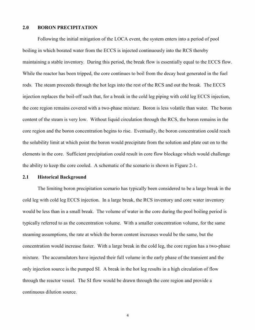
4-19) and into loop 4 (Figure 4-20) to proceed out the break. The penetration of flow into upper plenum
and core provides additional coolant as well as flushes the core region, which reverses the buildup of
boron.

40
Figure 4-8. 6.5 inch Cold Leg Break – System Masses

41
Figure 4-9. 6.5 inch Cold Leg Break – System Pressures

42
Figure 4-10. 6.5 inch Cold Leg Break – Core Power

43
Figure 4-11. 6.5 inch Cold Leg Break – SG Apex Flow

44
Figure 4-12. 6.5 inch Cold Leg Break – MHSI Flow

45
Figure 4-13. 6.5 inch Cold Leg Break – Accumulator Flow

46
Figure 4-14. 6.5 inch Cold Leg Break – Cold Leg LHSI Flow

47
Figure 4-15. 6.5 inch Cold Leg Break – Hot Leg LHSI Flow

48
Figure 4-16. 6.5 inch Cold Leg Break – Integrated Total Flow, Upper Head to Hot Leg

49
Figure 4-17. 6.5 inch Cold Leg Break – Integrated Total Flow, Core Exit
50
Figure 4-18. 6.5 inch Cold Leg Break – Integrated Total Flow, Core Inlet

51
Figure 4-19. 6.5 inch Cold Leg Break – Integrated Total Flow, Lower Head to Lower Plenum

52
Figure 4-20. 6.5 inch Cold Leg Break – Integrated Total Flow, Cold Leg to Downcomer

53
4.2 SBBP Model Inputs
4.2.1 Generic SBLOCA Boron Precipitation Analysis SBBP Model Inputs
The following inputs are generic to the two SBLOCA demonstration SBBP analyses:
• Initial power: 4612 MWth
• Initial RCS pre-LOCA enthalpy: 605.1 BTU/lbm for an average operating RCS temperature
and pressure
• Initial RCS boron concentration: 800 ppm
• Volume of stainless steel metal structures in concentrating region: 800 ft3
• Volume of non-stainless steel structures in concentrating region: 40 ft3
• Volume of fuel: 700 ft3
• Temperature-averaged volumetric heat capacity of stainless steel: 61 BTU/ft3-ºF (calculated
from time vs. value inputs)
• Temperature-averaged volumetric heat capacity of non-stainless steel materials: 31 BTU/ft3-
ºF (calculated from time vs. value inputs)
• Temperature-averaged volumetric heat capacity of UO2: 46 BTU/ft3-ºF (calculated from time
vs. value inputs)
• SI pump curves: Pressure vs. injection flow rates
• ABS injection flow rates: 0.25 ft3/s
o Assumed initiation: time zero (A sensitivity study is performed regarding this input,
Section 4.3.3.2)
• SI boron concentration: 2000 ppm
• ABS boron concentration: 7000 ppm
• Hot leg injection temperature: 130ºF

54
• Assumed Entrainment: 25% (A sensitivity study is performed regarding this input, Section
4.3.3.3)
• Flashing Option: On
• Stored Energy Option: On (A sensitivity study is performed regarding this input, Section
4.3.3.1)
4.2.2 Generic Concentrating Region Definition
The transient liquid volume in the concentrating region, i.e. the concentrating volume, is break
size dependent. However, the areas of the RCS which comprise the concentrating region is generic for
this SBLOCA demonstration. The concentrating region is defined based on the communication between
regions which exists during the pool boiling period (Figure 4-21). The recirculation pattern during the
pool boiling period will bring water from the lower plenum (between lower support plate and heated
core), into the core, into the upper plenum, and back down through the heavy reflector, guide tubes, and
peripheral core regions. The peripheral core region represents the lower powered regions of the core.
The downflow in these regions will also flow into the higher powered regions (as represented by the
central core) due to the differences in density. While the SBLOCA will have water inventory in the hot
legs that will participate in the mixing process, these volumes are conservatively neglected. The
SBLOCA concentrating region is therefore comprised of the regions from the “Lower Plenum” volume
up to and including the full “Upper Plenum” volume.

55
Figure 4-21. SBLOCA Pool Boiling Circulation Pattern
4.2.3 3 inch Transient Boron Precipitation Analysis Inputs
The key event times for the 3 inch break are:
• Time of reactor trip: 32 seconds
• Time of loss of natural circulation: 460 seconds
• Time of restart of natural circulation: 11000 seconds
The pressure, concentrating volume, and temperatures are approximated based on the results
from the S-RELAP5 transient analysis. Figure 4-22 through Figure 4-24 show the transient data and the
fitted curves used in the analysis. The fitted concentrating volume data conservatively neglects the
temporal increases in the liquid volume due to accumulator injection. The injection would dilute the

56
core with rapid injections of lower concentrated water and displace the higher concentrated water out to
the hot legs. The system refill begins around 7500 seconds, increasing the volume of water in the
concentrating region noticeably around 8000 seconds. Natural circulation restarts around
11000 seconds. The fitted data ignores the refill and continues the decreasing pressure trend to
atmospheric pressure. This results in a higher concentration and lower solubility limit.
0
500
1000
1500
2000
2500
0 1000 2000 3000 4000 5000 6000 7000 8000 9000 10000 11000 12000 13000Time (seconds)
Pres
sure
(psi
a)
RELAP PressureFitted Data
Figure 4-22. 3 inch Break Pressure Data

57
0
200
400
600
800
1000
1200
1400
1600
1800
2000
0 1000 2000 3000 4000 5000 6000 7000 8000 9000 10000 11000 12000 13000
Time (seconds)
Tem
pera
ture
(ºF)
RELAP Clad TempRELAP Fuel TempFitted Data
Figure 4-23. 3 inch Break Temperature Data
0
500
1000
1500
2000
2500
3000
3500
0 1000 2000 3000 4000 5000 6000 7000 8000 9000 10000 11000 12000 13000
Time (seconds)
Liqu
id V
olum
e (ft
³)
RELAPRELAP No HLFitted Data
Figure 4-24. 3 inch Break Concentrating Volume Data

58
4.2.4 6.5 inch Transient Boron Precipitation Analysis Inputs
The key event times for the 6.5 inch break are:
• Time of reactor trip: 6 seconds
• Time of loss of natural circulation: 120 seconds
• Time of restart of natural circulation: n/a
The pressure, concentrating volume, and temperatures are approximated based on the results
from the S-RELAP5 transient analysis. Figure 4-25 through Figure 4-27 show the transient data and the
fitted curves used in the analysis. The S-RELAP5 transient analysis assumed hot leg injection at 30
minutes and the fuel temperature and concentrating volume data from the transient run past 1800
seconds are irrelevant. The pressure is driven by the break and the controlled secondary side cool down.
Hot leg injection redirects the majority of the LHSI to the hot legs, but the flow rates are still pressure
dependent. The injection location does therefore not affect the RCS pressure and therefore the pressure
data is still relevant for the entire transient.

59
0
200
400
600
800
1000
1200
1400
1600
1800
2000
0 1000 2000 3000 4000 5000 6000 7000 8000 9000 10000 11000 12000 13000
Time (seconds)
Pres
sure
(psi
a)
RELAP PressureFitted Data
Figure 4-25. 6.5 inch Break Pressure Data
0
200
400
600
800
1000
1200
1400
1600
1800
2000
0 1000 2000 3000 4000 5000 6000 7000 8000 9000 10000 11000 12000 13000
Time (seconds)
Tem
pera
ture
(ºF)
RELAP Clad TempRELAP Fuel TempApproximation
Figure 4-26. 6.5 inch Break Temperature Data

60
0
500
1000
1500
2000
2500
3000
0 1000 2000 3000 4000 5000 6000 7000 8000 9000 10000 11000 12000 13000
Time (seconds)
Liqu
id V
olum
e (ft
³)
RELAPRELAP No HLFitted Data
Figure 4-27. 6.5 inch Break Concentrating Volume Data
4.3 SBBP Model Results
4.3.1 3 inch Boron Precipitation Analysis Results
The boron concentration is shown along with the assumed volume in Figure 4-28. It plots the
concentration on the left axis, the liquid volume used in the analysis on the right axis, and indicates the
time of key events with vertical lines. There is a very small increase in the concentration due to flashing
until the loss of natural circulation (+23 ppm). At that time, the pool boiling period begins and the
stored energy and decay heat steaming begin to steadily increase the boron content in the concentrating
region. Since the concentrating volume is held constant, the concentration also rises. Around 2000
seconds, the concentrating volume decreases and the concentrating rate increases. At 3500 seconds
when there is a jump in the concentrating volume, there is a concurrent reduction in the concentration.
Once the concentrating volume stabilizes, the concentration again begins its steady increase. Since the

61
increase in the concentrating volume at 8000 seconds was neglected, the initiation of LHSI does not
change the concentrating rate. The concentration and solubility limit for the 3 inch break is shown in
Figure 4-29. The solubility limit decreases in proportion to the decreasing saturation temperature
associated with the pressure reduction. Under the assumptions of the calculation, the 3 inch break would
reach the limit at approximately 13,300 seconds (3.7 hours). At this time the concentration reaches
38,500 ppm.
For this size break, the system can refill sufficiently to restart natural circulation which will act
to dilute and control the concentration. It was shown with the S-RELAP5 analysis that the LHSI would
refill the system and restart natural circulation around 11,000 seconds. Additionally, even if natural
circulation was not restarted the pressure drop assumed for the calculation is greater than would be
expected; with the size of the break and the continued LHSI, the system pressure would not be reduced
to atmospheric pressure and the solubility limit would remain above 38,500 ppm. At the time when
natural circulation restarted, the pressure is about 110 psia. This gives a limit of 67,600 ppm and a
margin greater than 33,000 ppm.
While natural circulation would be an effective mitigation of the concern of boron precipitation,
the emergency operating procedures may have already provided guidance to the operator to initiate hot
leg injection. Figure 4-30 shows the hot leg injection flow rates that would occur and the dilution
concentrations of these flows. Hot leg injection for this plant splits about 80% of the flow to the hot leg,
while 20% continues to inject into the cold leg. With the high hot leg injection flow rates there is excess
hot leg injection available to penetrate the highly concentrated core before 6500 seconds even with 25%
entrainment of the flow into the SGs. Therefore, it can be concluded that for this break size, either the
restart of natural circulation or the initiation of hot leg injection are capable of precluding boron
precipitation for this break.

62
4.3.2 6.5 inch Boron Precipitation Analysis Results
The results figures for the 6.5 inch break are presented in Figure 4-31 through Figure 4-33. A
comparison plot of the concentration vs. time and the solubility limit vs. time for the 3 inch break and
6.5 inch break is presented in Figure 4-34. A comparison plot of the margin between the concentration
and solubility limit for the two breaks is presented in Figure 4-35.
The loss of natural circulation for the 6.5 inch break is at 130 seconds, over 300 seconds sooner
than in 3 inch break. The pool boiling period begins at this time and the concentration rapidly begins to
rise. The concentration experiences a rapid decrease though when the system pressure reduces to the
point where the accumulators empty and the LHSI begins to inject. The additional injection causes an
increase in liquid volume. While the injection is borated, the increase in concentrating volume is more
dominant in determining the concentration. By 1000 seconds, the concentrating volume has stabilized
and the concentration starts to steadily rise. In reality, the decrease in decay heat and continued
injection of cold LHSI which leads to less voiding in the core would increase the concentrating volume.
However, consistent with typical boron precipitation analyses, the concentrating volume input was
assumed to be constant for the remainder of the transient evaluation (Figure 4-27). This assumption is
consistent with the typical LBLOCA boron precipitation analysis. The solubility limit decreases much
faster in the 6.5 inch break as compared to the 3 inch break because of the RCS pressure differences.
The 3 inch break required the cooldown via the SGs to reduce the RCS pressure (Figure 4-2) whereas
the break itself reduced the RCS pressure in the 6.5 inch break (Figure 4-9). The concentration and
solubility limit for the 6.5 inch break is shown in Figure 4-29. Under the assumptions of the calculation,
the 6.5 inch break would reach the solubility limit at approximately 12,300 seconds (3.4 hours). At this
time the concentration reaches 38,500 ppm.
For this break size and only two ECCS pumps, natural circulation would not restart before the
limit was reached. Hot leg injection would be required as the active dilution mechanism. Figure 4-33
shows the hot leg injection flow rates and dilution concentrations. Because the hot leg injection is

63
supplied via the pressure-dependent LHSI system there is more flow available earlier than in the 3 inch
break. Excess flow is provided before 1000 seconds for both the full flow and 25% entrainment
assumption. Hot leg injection would be effective, providing excess flow to penetrate downward, and
dilute the core, well before precipitation would occur.
4.3.3 Additional Sensitivities
The SBBP model has several options available to easily evaluate the impact of certain
assumptions. For instance, the contribution of stored energy can be neglected, the assumed hot leg
injection entrainment can be changed, and an LBLOCA can even be simulated.
4.3.3.1 Stored Energy Contribution
One of the concerns for the SBLOCA boron precipitation evaluation is that, unlike an LBLOCA,
the majority of the stored energy is not removed via the break. The heat release from the RPV and
internal metal structures would impact the solution. The stored energy was included in the modeling
and results described above. For the 3 inch break, when the stored energy is neglected the time of
precipitation changes from 13,338 seconds to 14,124 seconds. For the 6.5 inch break, the time changes
from 12,341 seconds to 12,912 seconds. This is a change of approximately 10 minutes for both cases.
4.3.3.2 Timing of ABS Initiation
One of the conservative assumptions made was the operator immediately starts any additional
boration sources. Immediately following the event, the operators would be concerned with protecting
the fuel and RCS integrity. The most important source of negative reactivity following the event is the
insertion of the control rods. Only later in time would the focus be turned to additional boration and
only as the emergency operating procedures would direct. Instead of assuming that ABS injects from
time zero, it is assumed that the operators initiate it at 30 minutes. For the 3 inch break the time to the
limit increases by 820 seconds. For the 6.5 inch break the time increases by 480 seconds. The effect is
64
more pronounced with the smaller break since the higher pressures reduce the pumped injection. Since
the injection concentration is flow rate weighted, with less flow from the lower concentrated fluid, the
injection concentration with an ABS is higher. Figure 4-36 demonstrates this. It is important to note
that for the smaller breaks, like the 3 inch break, an ABS is more important due to the restart of natural
circulation and potential boron dilution event which could occur at that time.
4.3.3.3 Hot Leg Injection Entrainment
Once the hot leg injection flow can remove the heat through boiloff, there is excess flow
available to penetrate into the concentrating region, thereby diluting the core and displacing the highly
concentrated water out to the break. Early in the transient, the decay heat is the dominant contributor.
The decay heat is independent of break size, but the HLI system is supplied via the pressure-dependent
LHSI system and therefore the smaller the break, the higher the pressure, and the longer until there is
excess HLI. For the 3 inch break, there is excess flow available at ~5900 seconds after reactor trip if
there is no entrainment. If there is 25% entrainment, it will take until ~6100 seconds after reactor trip.
Even with 80% entrainment, excess flow is available at ~8400 seconds after trip. The excess flow at this
time would not be very high and due to the boiloff, its concentration would be elevated, as can be seen
in Figure 4-37. This calculation conservatively assumes that all of the energy is going to the boiloff of
the ECCS injected in the hot leg. The energy cannot simultaneously be boiling the water in the core and
the boiloff. However, even with this assumption, by the predicted time of precipitation (13,300
seconds), the excess flow would be approximately 50 lbm/sec and have a concentration less than 20,000
ppm.
4.3.3.4 Inclusion of the Liquid Volume in the Hot Legs
In August of 2010, a boron precipitation test, Test G5.1, was conducted at the PKL III test
facility. It was a parameter study on the influence of core power, ECC injection rates, and hot leg
injection on boron concentration in the core during the long-term cooling period following a large break

65
LOCA in the cold leg. The results from the test clearly indicated that the volumes which mix would
include more than just the core region. As the mixing defines the concentrating region, the
concentrating volume would be larger than assumed. An evaluation of the rates at which the
concentration increased indicated that the concentrating volume would need to include the hot legs and
SG inlet plenums in order to obtain the reported concentrations when solutions with water and boric acid
were in these regions (Ref. [15]).
The demonstration analyses did not include the hot leg liquid volume in the determination of the
time to the solubility limit (Figure 4-24 and Figure 4-27). Inclusion of the hot leg liquid volume in the
concentrating region adds approximately 200 ft3 to the concentrating volume. The result is shown in
Figure 4-38 and Figure 4-39 for the 3 inch and 6.5 inch break respectively. The time to the solubility
limit exceeded the time steps included in the tool. A linear extrapolating of the rate at the last available
time step is used to calculate the time to the solubility limit. For the 3 inch break, the time to the limit
was extended from 13,338 seconds to 17,385 seconds. For the 6.5 inch break, the time to the limit was
extended from 12,341 seconds to 16,715 seconds. For both breaks, this is an increase in the available
timing for mitigative action by over an hour. This well dwarfs the assumptions of ABS and stored
energy. However for use in a licensing calculation, the inclusion of the liquid volume in the hot legs
would have to be more strongly supported by definitive experimental results.
4.3.3.5 LBLOCA Simulation
Historically, boron precipitation analyses assume that the LBLOCA scenario is bounding, but
this was one of the criticisms from the NRC (Section 2.1). As such this thesis explicitly analyzes the
SBLOCA event. The evaluation method described herein uses the characteristics of the SBLOCA event,
based on S-RELAP5 simulations, to calculate concentrations and solubility limits as a function of time.
This is in opposition to the more typical LBLOCA analysis which only relies on a single mixing volume
and a single pressure assumption for the entirety of the event. The Excel tool can however be used to

66
simulate this simpler LBLOCA analysis. A reactor trip and loss of natural circulation are assumed to
occur at 1 second. The mixing volume at 1 second is set to 500 ft3 and held constant. The pressure at 1
second is set to 14.7 psi and held constant. The initial concentration in the boiling pot mode is the
injection concentration since in an LBLOCA the system will rapidly empty and be refilled by the
accumulators and pumped SI. As such the Flashing Option provided in the tool is turned off and an
initial concentration equal to the assumed injection concentration (2000 ppm) is used. Also, in an
LBLOCA the majority of the stored energy is removed via the break; the Stored Energy Option in the
tool is turned off.
The results of the LBLOCA simulation are shown in Figure 4-40. The solubility limit of 38,500
ppm is constant throughout the transient due to the pressure assumption. The rate at which the
concentration rises is also directly proportional to the decay heat since the volume and latent heat of
vaporization are constant. The LBLOCA reaches the solubility limit at ~5500 seconds (1.5 hours)
(Figure 4-40). Under those assumptions, the LBLOCA is clearly more bounding with respect to the time
at which hot leg injection must be initiated. However, because the pressure is below the shutoff head of
the LHSI, which provides the HLI, the HLI exceeds the decay heat before an hour.
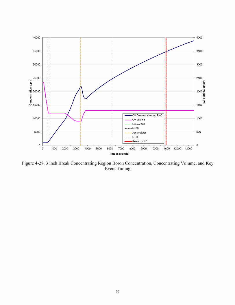
67
Figure 4-28. 3 inch Break Concentrating Region Boron Concentration, Concentrating Volume, and Key
Event Timing

68
Figure 4-29. 3 inch Break Concentrating Region Boron Concentration and Solubility Limit

69
Figure 4-30. 3 inch Break Hot Leg Injection Effectiveness

70
Figure 4-31. 6.5 inch Break Concentrating Region Boron Concentration, Concentrating Volume, and
Key Event Timing

71
Figure 4-32. 6.5 inch Break Concentrating Region Boron Concentration and Solubility Limit

72
Figure 4-33. 6.5 inch Break Hot Leg Injection Effectiveness

73
Figure 4-34. Concentration and Solubility Limit Comparison - 3 inch and 6.5 inch Break

74
Figure 4-35. Margin Comparison - 3 inch and 6.5 inch Break

75
Figure 4-36. Injection Concentration Comparison - 3 inch, 6.5 inch, and Large Break

76
Figure 4-37. 3 inch Break with 80% Entrainment

77
Figure 4-38. 3 inch Break with and without Hot Leg Volume

78
Figure 4-39. 6.5 inch Break with and without Hot Leg Volume

79
Figure 4-40. LBLOCA Concentrating Region Boron Concentration and Solubility Limit

80
5.0 BORON DILUTION
During certain SBLOCAs, the RCS inventory is reduced but the pressure of the primary side
remains equal to or above that of the secondary side. In this scenario, the SGs remove decay heat from
the RCS through reflux condensation. Water is boiled in the reactor core and the steam is condensed in
the SGs tubes. Because boric acid is not as volatile as steam, boron tends to be concentrated within the
reactor vessel core region. Then, the steam condenses in the SGs resulting in water with a reduced
boron downstream of the SG outlet plenum. The deborated water can potentially accumulate and, upon
the restart of natural circulation, be transported toward the core. The entry of water into the core with a
reduced boron concentration could cause a recriticality. This event, referred to as inherent boron
dilution, was identified by the NRC as Generic Safety Issue (GSI)-185.
5.1 Historical Background
During the mid-nineties, it was found that for B&W-designed PWRs a large amount of deborate
could be generated during the reflux-condenser mode of operation following an SBLOCA event (Ref.
[16]). The B&W design allowed for a large volume of the deborate to accumulate. The accumulated
deborate is typically referred to as a deborated slug. If the deborated slug is transported to the core and
adequate reboration or mixing did not occur, a recriticality could occur. The transport could occur due
to a restart of natural circulation or a restart of the RCPs. The concern was established as GSI-185 in
Reference [17] in 2000.
The concern was evaluated for the operating plants by the vendors and the Office of Nuclear
Regulatory Research. The issue was subsequently closed in 2005 as documented in the Reference [18]:
the evaluations showed that in the event of a restart of natural circulation the Westinghouse and CE
plants would remain subcritical. The B&W reactor had the largest accumulation of deborate. Analyses
were performed which demonstrated that a recriticality would occur but that there was no fuel damage.
Therefore, it was determined that “boron dilution with restart of natural circulation is not a significant

81
event at all Westinghouse, Combustion Engineering, and Framatome B&W reactors (Ref. [18]).”
Emergency operating procedures were developed to deal with the RCP restart scenario.
Initially there were few experiments dedicated to the subject, but with the increased attention,
more tests were convened. Inherent boron dilution tests typically focus on two aspects of the event
separately: (1) the thermal hydraulic phenomena involved in the generation of the slug, and (2) the
mixing of the deborated slug with the higher concentrated fluid from the ECCS injection and in the
downcomer (Ref. [19]). The thermal hydraulic phenomena can be transposed, with adequate
justification, to different plant designs. The mixing is more difficult to quantitatively apply directly to
other plant designs. Mixing experiments can instead be used for benchmarking computational fluid
dynamics (CFD) models which then can be applied to specific plant designs. The most extensive series
of tests on the thermal hydraulic phenomena was performed in the PKL facility (Ref. [20]).
5.2 SBLOCA Boron Dilution Analysis
While the issue was closed for operating plants, it must continue to be demonstrated that plant
changes do not invalidate the closure and that new plant designs will not challenge the criteria
established by the NRC in an inherent boron dilution event. For new plant designs, such as the U.S.
EPRTM plant, attention must be paid to the higher reactor powers and the particular details of the
emergency safety equipment configurations. With more power, the decay heat generated following a
reactor trip is greater creating more steam which, if condensed, could lead to greater volumes of
deborate. The ECCS design configurations can introduce different failure scenarios which could affect
reboration. This thesis presents an analytical methodology which can be used to evaluate the inherent
boron dilution event for a PWR with U-tube SGs and cold leg ECCS injection.

82
6.0 BORON DILUTION ANALYTICAL METHODOLOGY
While the true criteria for this event is the maintenance of long-term core coolability and the
prevention of fuel damage (10 CFR 50.46 (Ref. [1]); GDC 28, (Ref. [21], Ref. [18]), a conservative
decoupling criterion of no return to criticality is used. In order to assess the potential for recriticality
during the inherent boron dilution event a combination of experimental test results, system code
analyses, and CFD analyses are used. A schematic of the approach is shown in Figure 6-1. The PKL
test facility investigated the thermal hydraulic phenomena associated with the event (Ref. [20]).
System code analyses evaluate the particular performance of the plant and the effects of break size and
systems availabilities on the transient evolution in order to determine limiting scenarios up until the
restart of natural circulation (RNC). Mixing tests and CFD analysis are then used to evaluate the mixing
process during transport following the RNC. CFD analyses, when validated by tests, are capable of
accurately simulating the mixing processes in the cold legs, downcomer, and lower plenum, and
determining the boron concentration at the core inlet. The minimum boron concentration at any location
at the core inlet is then compared to critical concentration, as determined with a neutronics analysis, to
ensure that there is no return to criticality. The use of this criterion represents a large conservatism in
preventing recriticality. It neglects the large variations in the boron concentration across the core inlet,
the increased concentration in the core, and the mixing in the core.
6.1 Event Description
The first step in establishing an analytical methodology is to establish the event progression and
key event phenomena. There is a particular range of break sizes which are susceptible to this event.
The initiation of a break in the RCS large enough that cannot be compensated by system makeup leads
to the draining of the system. As inventory and energy are released through the break the primary
pressure decreases. A reactor trip signal is sent when the low pressurizer pressure setpoint is reached.
The RCPs are tripped either at reactor trip, based on assumed LOOP, by an automatic RCP trip signal,
or by operator action, at which time the pumps begin to coast down. The pressure and the water level

83
continue to decrease in the pressurizer and when the conditions of saturation are reached, first in the hot
regions of the RCS, the reactor coolant vaporizes, starting a period of two-phase circulation. Depending
on the break size, this period is followed by a transition to single-phase steam flow. For the smallest
breaks, the primary pressure stabilizes above the secondary pressure in which case the SGs function to
remove energy from the primary. When this happens, the steam condenses and can accumulate
downstream of the SG as a slug of water with a reduced boron concentration. For larger breaks, the
primary pressure can become lower than the secondary pressure. In this case, the SGs only remove heat
when the cooldown results in a sufficient pressure reduction. Eventually, if the system is sufficiently
refilled by the ECCS, natural recirculation can restart. If this occurs, the deborated slug passes towards
the core inlet through the cold legs and downcomer. If the transport of the slug results in a reduced
concentration in the core, a recriticality could occur.
6.2 Physical Phenomena Relative to the Boron Dilution Event
Contrary to the classical evaluation of SBLOCA transients which are particularly interested in
the core uncovery phase, the SBLOCA transients for the boron dilution event have a longer duration,
lasting from one to six hours, depending on the break size and cooldown rate. There are four
characteristic phases of the accident relative to the evolution of the boron dilution event:
6.2.1 Transition from Forced Circulation to Two-phase Natural Circulation
The phase of forced circulation comes to an end after the shutdown of the reactor coolant pumps.
The draining of the RCS continues because the break flow exceeds any external compensation. This
progressive draining causes greater evaporation of the water due to a reduced flow rate to the core. The
steam flow increases to the SGs, but water is still entrained with the high steam flows. This is the two-
phase natural circulation period in which there is continuous flow of liquid over the SG apex and
through the system. Any condensate generated in the tubes of SGs is mixed with the borated water in the
RCS. The natural circulation flow maintains a rather homogeneous boron concentration in the RCS.

84
6.2.2 Interruption of Natural Circulation
For large enough break sizes, the loss of system inventory is sufficient to cause the interruption
of natural circulation. First a period of intermittent flow arises in which liquid continues to be carried
over the SG apex with the steam flow. As the system inventory continues to decline, a complete
interruption of natural circulation occurs. It is indicated by the loss of liquid flow at the SG tube apex.
According to the PKL test results (Ref. [20]), the accumulation of deborate during this phase begins
when the RCS liquid level falls below that of the SG tube bundle at the SG outlet. The very weakly
borated steam produced in the core passes through the hot legs into the SG tubes where it is condensed.
This mode of heat transfer by evaporation/condensation is characteristic of a low system inventory and
requires the cooldown by the secondary side. The liquid resulting from the condensation on the upsides
of SG tubes falls back, countercurrent to the steam flow, towards the upper plenum mixing again with
the borated water in the SG inlet plenum, hot legs, and core. The PKL test results demonstrated that
there was no accumulation of highly deborated liquid in the SG inlet plenum. On the other hand, the
accumulation of deborate in the SG outlet plenum and loop seal could lead to the formation of deborated
slugs.
6.2.3 Refill and Resumption of Natural Circulation
The filling of the reactor coolant system is achieved, for the smaller breaks, by MHSI alone; or
for the larger breaks, by the addition of the accumulators and/or the LHSI. Once the level reaches the
bottom of the SG tubes at the SG outlet; the carryover of liquid, as demonstrated in the PKL test results,
ends the phase of deborate accumulation. The refill of the RCS results in a phase of intermittent flow
followed by a resumption of continuous natural circulation. The restart of natural circulation is
necessary for the transport of the deborate towards the reactor and the challenge to recriticality. The
phenomena in the refill phase leading up to the restart and the restart dynamics are discussed in more
detail in Section 6.3.1.

85
6.2.4 Transport of Deborate towards the Core Inlet
The final phase of the event is the transport of the deborated slug to the core inlet. During this
movement, the slug mixes in the cold legs with borated water injected from the SI and accumulators and
ABS, if present, and finally with the borated water in the downcomer and lower plenum. This mixing
raises the boron concentration before it reaches the core.
6.3 PKL Tests
The PKL test facility is based on a typical four-loop PWR of German design (Ref. [20]). The
entire primary side, the most significant components of the secondary side (excluding the turbine and
condenser), and the appropriate system technology, are represented (Figure 6-2). The major component
heights on the primary and secondary side are scaled with a 1:1 ratio to the reference plant. The
volumes, power, and mass flows are scaled with a ratio of 1:145. For some components, the exact
volume scaling is not applied in order to simulate certain thermal hydraulic phenomena; for example,
counter current flow limitation in the hot legs. This allowed dimensionless numbers (e.g., the Froude
number) to be maintained in the correct parameter range. Due to its full-scale height and symmetric
layout of the four loops, the PKL test facility is well suited for the study of reflux condensation and
natural circulation phenomena.
Four tests relevant to the inherent boron dilution event were conducted with the PKL III E and F
test series. Test E2.2 and Test F1.1 were transient simulations. Test E2.2 simulated a cold-leg break
with asymmetric cold-leg injection from only two safety injection pumps. The test had a very long
reflux condenser period and excessive condensate production in order to obtain the maximum possible
volume of accumulated condensate. Test F1.1 also simulated a cold-leg break, but with symmetric
cold-side injection into all four loops. A major focus of this test was to investigate the potential for
simultaneous restart of natural circulation. Test F1.2 and Test F4.1 were parametric studies that
investigated the relationship between the primary inventory drain and refill and the start and end of

86
reflux condensation and condensate accumulation. The matrix of tests allowed for conclusive findings
to be made relative to the boron dilution processes and to the refill and restart of natural circulation.
While Test E2.2 had a long condensation period, the refill and restart of natural circulation
processes limited the amount of condensate which could accumulate as a slug. [
] As soon as the refill allows for a level above the SG outlet side tube sheet,
transport phenomena over the SG apex enable further disintegration and reboration of the slug. These
transport phenomena were investigated in detail and confirmed with the parametric study tests, Test F1.2
and Test F4.1. Therefore, the size of the slug is limited to the loop seal and SG outlet plenum.
The tests also concluded that natural circulation arises in different loops at different times due to
the inherent asymmetries between the tubes of a single SG and between the refill processes of the
individual loops. Test E2.2 demonstrated that the loop which restarts first is a loop without injection.
The colder water in the loop seal of the loops with injected ECC creates a temperature and density
difference which delays the restart of natural circulation. The restart of natural circulation in one loop
causes a decrease in the steam production, which reduces the swell levels in the SGs of the other loops
and delays the restart of natural circulation in those loops. [
] The following loops start with considerably lower flow rates,
corresponding to typical single phase flows. Test F1.1, which was set up for the most symmetric
boundary conditions, confirmed the single loop restart and delay to restart of natural circulation in the
other loops.
The main conclusions from the test matrix are:

87
• In order for the accumulation of condensate, the water level must be below the SG outlet tube
sheet.
• The size of the deborated slug is limited to the volume of the loop seal and the SG outlet.
• The exchanges between the SG inlet plenum, hot leg, upper plenum, and core region prevent the
formation of a deborated slug on the SG upside.
• Natural circulation does not restart simultaneously, regardless of whether ECC injection is
symmetric or asymmetric.
• Natural circulation restarts first in loops without ECC.
• The first restart of natural circulation impedes the restart of natural circulation in subsequent
loops.
• During the refill phase, there are intermittent flows of borated water from the cold leg back into
the loop seal and from the inlet SG plenum, over the SG tubes apex. These flows mix, reborate,
and partly disintegrate the deborated slug prior to its transport towards the core.
• Weakly borated slugs were observed only in loops without ECC.
A more detailed description of the evolution of the system refill, restart dynamics, and the
thermal-hydraulic phenomena that limit the slug size and preclude multiple restarts is provided in the
Section 6.3.1, as evidenced in the PKL tests.
6.3.1 Refill and Restart Dynamics
The tests in the PKL boron dilution matrix allowed for an in-depth understanding of
characteristics and thermal-hydraulic processes which occur during the system refill and lead up to the
restart of natural circulation.
[
]

88
[
]

89
[
]

90
[
]
6.4 System Code Analyses
Many thermal-hydraulic aspects of boron dilution, except the mixing effects, can be analyzed by
using system codes such as CATHARE and S-RELAP5. The mixing processes from the loop seal to the
core involve multidimensional flow effects which typically are not modeled in system codes.
Furthermore, these codes exhibit far too much numerical diffusion to be useful for tracking a relatively
sharp concentration gradient around the system (Ref. [22]). Such system code analyses are used to look
at the overall system evolution as a result of break sizes in the range of concern. The depletion and refill
characteristics of the transient are well captured by system codes. Since the timing of the different
phases in the boron dilution event evolution are dependent on the system inventory, system codes can be
used to provide an indication of the critical times in the event. The system characteristics: pressure,
temperature, flow rates, etc. at these times are relevant. The condensation in SGs during the phases can
also be captured by the system code analyses. Additionally, system code analyses can provide a means
to compare the effects of different break sizes, equipment availabilities, and operator actions.

91
6.5 CFD Analyses
Once a limiting scenario has been identified with the conclusions from the experimental tests and
plant-specific system code analyses, the transport phase and the mixing that occurs in the cold leg,
downcomer, and lower plenum during the transport are evaluated with CFD analyses. CFD analyses
have been proven to be an effective tool for calculating three dimensional mixing flows, but the applied
numerical methods and turbulence models require experimental validation with detailed local resolution
of flow and temperature fields. The CFD models are very plant-specific since they model the explicit
geometry of the plant. The results are also case-specific as the mixing can vary greatly with different
conditions and configurations. In order to analyze the event efficiently, extreme care must be taken
when defining the bounding scenarios to be analyzed.
The CFD analyses simulate the transport of the deborated slug and the mixing between the slug
and the surrounding borated water in the cold leg, downcomer, and lower plenum in order to determine
the local distribution of boron concentrations at the core inlet as a function of time. The concentration
results of the CFD analyses are compared to the critical concentration to assess the potential for a core
recriticality. If the CFD analyses demonstrate that the concentration at the core inlet is greater than the
critical concentration then the potential for recriticality is eliminated. Alternatively, if the minimum
concentration is not above the critical concentration, the distribution of the concentrations can be passed
to a coupled thermal-hydraulic-neutronic analysis to demonstrate that there is no fuel damage. This
alternate approach is in line with the B&W analyses that were used to close GSI-185 for operating plants
(Ref. [18]).
The boundary conditions for the CFD analyses are based on the combination of the system analyses
and the PKL conclusions. The assumptions regarding the restart sequence (one loop without ECC), slug
size (loop seal plus SG outlet plenum), and slug flow rate are based on the PKL test conclusions. Even
though reboration of the slug volume prior to the transport of the slug was evidenced in the tests, for a
plant-specific application the amount of reboration would be difficult to quantify. Instead, this

92
pre-transport reboration can be conservatively neglected. The conditions that are supported by system
analyses include:
• Pumped injection flow rates.
o While the accumulators may or may not be isolated, the amount and timing would be
difficult to accurately define. As such, they can be conservatively neglected.
• Injection concentrations.
• Initial RPV temperature.
• Initial RPV concentration.
• Slug temperature.
6.6 Conservatisms
The approach for evaluating the inherent boron dilution event contains a number of large
conservatisms in addition to the conservatisms which are included in the analysis inputs. The
conservatisms of the approach and analyses include:
• Criterion of no recriticality is used while the true criteria are maintaining long-term core cooling
and preventing fuel damage.
• The comparison of the minimum concentration at any location across the core inlet to the core-
wide critical concentration is conservative because it neglects the distribution of higher boron
concentrations across the core inlet and neglects the mixing in the core where the concentrations
are increased.
• The CFD analyses neglect accumulator injection.
• The slug volume is equal to the total liquid volume between the SG outlet tube sheet and the cold
leg discharge piping. The slug concentration is minimized. These assumptions neglect the
intermittent flows period prior to the restart of continuous natural circulation which reborates and
partially disintegrates the slug.

93
Figure 6-1. SBLOCA Inherent Boron Dilution Analytical Methodology

94
Figure 6-2. PKL III Test Facility

95
7.0 DEMONSTRATION OF BORON DILUTION ANALYTICAL METHODOLOGY
Consistent with the SBBP model demonstration (Section 4.0), a 4-loop PWR with 4 independent
ECCS trains, an additional boration source, and an operator initiated cooldown was analyzed using the
methodology described herein. The first step was to analyze the plant’s design (ECCS, operator actions,
etc.) to determine a set of potentially limiting boron dilution scenarios. The scenarios are examined first
from the perspective of in-loop reboration (referring to the borated systems in the loop which restarts
natural circulation first), then total system boration, then available EFW. Once this was done, a
comprehensive set of S-RELAP5 cases was analyzed to determine the effect of break size, equipment
availability, and operator actions on the transient evolution. The depletion and refill characteristics of
the transient are well captured by the system code. Since the timing of the different phases (forced flow,
intermittent two-phase flow, single-phase steam) are dependent of the system inventory, S-RELAP5 was
used to give an indication of these times. The system characteristics, pressure, temperature, flow rates,
etc. at these times are relevant to the event. Additionally, S-RELAP5 was used to evaluate condensation
in the SG during these time periods.
Figure 7-1 and Figure 7-2 show some example comparisons that were used in the break size
spectrum sensitivity. Some additional parameters of comparison include per-loop condensates, time
between loss and restart of intermittent flow, pressures and temperatures, the injection flow rates at
RNC, the amount of boron injected up to RNC. An additional calculation is performed outside of
S-RELAP5 to determine the downcomer boron concentration at the time of RNC.
The results of the system analysis studies showed that there was a range of break sizes which
would result in the loss of intermittent flow over the SG apex, but that would not depressurize the
primary below that of the secondary. The upper end of the break size and possible ECCS combinations
is also limited by those scenarios which restart in natural circulation. If no restart of natural circulation
occurs, the deborate cannot be rapidly transported to the core to challenge recriticality. The most
penalizing plant configurations have minimum additional boration sources, a longer-operator initiated

96
cooldown, and EFW available on all four SGs. This minimizes the boron injected into the system and
maximizes the system condensation, resulting in the lowest concentration in the downcomer at the time
of RNC.
Based on the conclusions of the system analysis studies a limiting scenario was selected to
provide the inputs for the CFD analyses. In this scenario all four SG are fed with EFW, but only three
trains of SI are available. A slower operator initiated cooldown is performed, consistent with a single
failure resulting in a reduced ABS injection flow rate. This extends the time to refill and restart of
natural circulation. Additionally, due to the reduced ABS flow rate, less boron has been injected at the
time of RNC. The slug is assumed to restart in the loop, which has no direct borated injection, but does
have EFW. The break size is large enough to result in an extended period of time between the end of
and restart of intermittent flows; thereby maximizing the condensate, but small enough for the refill to
occur without LHSI.
In this case, the RCS pressure (Figure 7-3) reaches the low primary pressure setpoint at
101 seconds and the reactor is tripped. With an assumed loss of offsite power, the pumps trip and forced
circulation stops. Steam is produced in the core and a period of two-phase natural circulation begins.
Any condensate generated during this period is borated by the continued circulation of liquid flow
through the system. The RCS pressure continues to fall and reaches the low-low primary pressure
setpoint at 710 seconds which actuates the SI system and initiates the automatic partial cooldown. The
MHSI flow increases as pressure decreases, but it is not enough to compensate yet for the flow out the
break. The RCS inventory continues to decline (Figure 7-4) and continuous natural circulation is lost at
~1300 seconds (Figure 7-5). A period of intermittent flow begins in which the high steam flow rates
continue to carry borated liquid over the SG apex and mix with any condensate. At ~2000 seconds,
intermittent flow stops and the period of single-phase steam flow begins (Figure 7-5). This begins the
reflux condensation period during which deborated condensate could accumulate as a slug below the SG
outlet tube sheet. The RCS continues to cooldown and depressurize due to the operator-initiated

97
cooldown following the completion of the automatic partial cooldown. The ECC flow eventually
exceeds the break flow rate due the increase in MHSI flow and the contribution from the accumulators.
The minimum RCS mass occurs at ~4300 seconds and the system refill begins (Figure 7-4). Intermittent
flow, in which borated liquid is carried over the SG apex, starts at ~9,300 seconds (Figure 7-5). Further
increases in the RCS level lead to the conclusion of the intermittent flow period and the first restart of
continuous natural circulation at ~11,600 seconds (Figure 7-5).
The injection flow rates, injection concentrations, initial RPV temperature, and initial RPV
concentration are used to set the boundary conditions of the CFD analysis. The actual inputs to the CFD
are bounding of the results from the system analysis. The PKL test results extrapolated to the plant’s
geometry define the slug size and restart kinetics. The CFD analyses are outside the scope of this thesis,
but an example of CFD results due to the transport of a deborated slug is shown in Figure 7-6 and Figure
7-7 (Ref. [23]). Neutronics analyses determined the critical concentration at the expected system
conditions for this plant. The minimum concentration at any single point in Figure 7-7 was shown to be
greater than the minimum core-wide concentration for recriticality. Therefore, there is no safety concern
in the inherent boron dilution event for this plant design.

98
Figure 7-1. RCS Mass for Different SBLOCA Break Sizes

99
Figure 7-2. Downside Condensate for Different SBLOCA Break Sizes

100
Figure 7-3. Boron Dilution Scenario: Primary and Secondary Pressures

101
Figure 7-4. Boron Dilution Scenario: RCS Inventory

102
Figure 7-5. Boron Dilution Scenario: SG Apex Liquid Flow

103
Figure 7-6. Example CFD Results - Minimum and Average Core Inlet Concentrations

104
Figure 7-7. Example CFD Results at Minimum Inlet Concentration Time

105
8.0 CONCLUSIONS
Following an SBLOCA and reactor trip, the core can continue to boil due to the decay heat. The
steam generation in the core results in an increasing boron concentration in the core regions. Without
termination of the steaming the boron concentration could rise above the solubility limit, causing boron
precipitation. The steam generated in the core proceeds through the hot legs to the SGs. For certain
SBLOCA where the pressure of the primary is equal to or above that of the secondary, the SGs condense
the steam, which is virtually boron free. An accumulation of the condensate can result in a deborated
slug downstream of the SG outlet. If a restart of natural circulation occurs, this could result in a
recriticality. Both boron precipitation and boron dilution can challenge long-term core cooling. While
both events occur within the SBLOCA break spectrum and are a result of continued core steaming, two
separate analytical methodologies are necessary to demonstrate that long-term core cooling is
maintained. Both analytical methodologies rely on transient system analyses to supply the inputs to and
justification of the follow-on calculation of boron concentrations.
8.1 SBLOCA Boron Precipitation Conclusion
Typical boron precipitation analyses assume that the large break is bounding for the boron
precipitation scenario. The analyses for LBLOCA boron typically use simplifying assumptions such
that the only transient characteristic of the analysis is decay heat. The characteristics important to boron
precipitation are more variable in an SBLOCA and therefore the use of many of those simplifying
assumptions is not appropriate. An analytical methodology and tool have been developed to explicitly
analyze the SBLOCA boron precipitation scenario. The method utilizes system analyses to provide the
transient inputs. A demonstration of the tool was provided for a 3 inch and 6.5 inch break in a
Westinghouse-type 4-loop PWR. It was shown that the transient characteristics of the event must be
considered when analyzing the SBLOCA boron precipitation scenario. The stored energy contribution
must be included as it increases the steaming rate and decreases the time to the limit. With a constant
flow-high concentration boration source, the flow rate weighted injection concentration is substantially

106
greater for small breaks than for large breaks due to the reduced pressure dependent SI flow.
Additionally due to the higher system pressures, the effectiveness of hot leg injection is a critical
component in the SBLOCA analysis. So even though this particular plant showed that the larger small
breaks were more bounding and that the traditional LBLOCA analyses was even more bounding, the
analysis of the SBLOCA event cannot be neglected. Different plant designs and operator actions could
result in situations where the SBLOCA boron precipitation scenario was more limiting.
The analytical methodology and tool developed herein can be applied to any SBLOCA event, for
any plant. The tool was implemented in Excel which was helpful for the development of each of the
SBLOCA particular contributions and debugging. However now that it has been developed, it would be
cleaner to have the tool developed as a computer program with a code such as Python. A separate Excel
workbook would not be required for each analysis. The user would still be required to provide the same
inputs, but the interface would be cleaner. More importantly, by writing a program, it would be easy to
assure that the same formulas are applied in every analysis whereas with using multiple Excel
workbooks errors can be easily introduced and go undetected.
It is also recommended that the analytical methodology and tool be evaluated for different plant
designs and different operator actions. This demonstration used a plant feature which allows the
operator to reduce the RCS pressure. Had this action not been taken the solubility limit would have
been higher, but the system may not have refilled and restarted natural circulation prior the time that the
concentration reached the solubility limit. Additionally, the plant had a very high hot leg injection flow
rate. A plant design with less flow may not be able to penetrate and dilute the core region. By
evaluating different plant designs, the robustness of the analytical methodology and tool can be
evaluated.
8.2 Boron Dilution Conclusion
A methodology to evaluate the inherent boron dilution scenario and a demonstration of that
methodology have been presented. The methodology involves the use of test results, systems analyses,

107
CFD, and neutronics analysis. The test results, when justified to the particular plant application, define
the limitations of the slug size and the restart kinetics. The system analyses define the other system
conditions, including downcomer parameters and injection configurations. The inputs to the CFD
analyses are set to be bounding of those conditions. The result of the CFD analysis, the core-inlet
concentration as a function of time, is used in combination with neutronics analysis. A conservative
decoupling criterion can be used to demonstrate that there is no return to criticality: if the minimum
concentration at any location at any time is greater than the critical concentration, it is demonstrated that
there is no threat of recriticality and no safety concern in the SBLOCA inherent boron dilution event. If
this decoupling criterion is not met, a CFD analysis incorporating the core and its elevated
concentrations could be performed to demonstrate that upon entering the core, the mixing elevates the
concentration. Alternatively, the core-inlet distribution could be used in a coupled thermal
hydraulic-neutronics analysis to show that if a recriticality did occur, there was no fuel damage.

108
REFERENCES 1 “Acceptance criteria for emergency core cooling systems for light-water nuclear power reactors.” Code of
Federal Regulations Title 10, Pt. 50.46, 2007 ed.
2 Tuunanen, J. et al., “Experimental and Analytical Studies of Boric Acid Concentrations in a VVER-440 Reactor during the Long-Term Cooling Period of Loss-of-Coolant Accidents.” Nuclear Engineering and Design 148 (1994): 217-231.
3 Y, Ogata Letter to J. Ciocco “MHI's Response to US-APWR DCD RAI No. 706-5339 Revision 0 (115.06.05).” 28 Apr. 2011. (ADAMS Accession Number: ML11132A053)
4 Westinghouse Electric Company LLC, WCAP-17360-NP “Small Scale Unbuffered and Buffered Boric Acid Nucleate Boiling Heat Transfer Tests with Sump Debris in a Vertical 3x3 Rod Bundle.” May 2012. (ADAMS Accession Number: ML12167A434)
5 PWR Owners Group “PWR Owners Group: Path Forward for Addressing Boric Acid Precipitation to Support GSI-191 Closure (NRC Meeting, March 7, 2012).” 7 Mar. 2012. (ADAMS Accession Number: ML12083A004)
6 AREVA NP GmbH Document, PCTCP-G/2010/en/0008 Revision B “PKL III G5.1 Investigations on Boron Precipitation after Large Break LOCA – Quick Look Report” Feb. 2011.
7 “AGREEMENT ON THE OECD/NEA PKL Phase 3 PROJECT To address thermal-hydraulic safety issues for current PWR and new PWR design concepts through experiments in the integral test facility PKL.” n.p., n.d. PDF file. Retrieved from http://crz.gov.sk/index.php?ID=603&doc=582891&text=1
8 R. Gramm Letter to J. Gresham “Suspension of NRC Approval for Use of Westinghouse Topical Report CENPD-254-P, ‘Post-LOCA Long-Term Cooling Model,’ Due to Discovery of Non-Conservative Modeling Assumptions During Calculations Audit.” 1 Aug. 2005. (ADAMS Accession Number: ML051920310)
9 D.S. Collins Letter to G. Bischoff “Suspension of NRC Approval for Use of Westinghouse Topical Report CENPD-254-P, ‘Post-LOCA Long-Term Cooling Model,’ Due to Discovery of Non-Conservative Modeling Assumptions During Calculations Audit (TAC NO. MB1365).” 23 Nov. 2005. (ADAMS Accession Number: ML053220569)
10 Westinghouse Electric Company LLC, WCAP-17047-NP, Revision 0 “Phenomena Identification and Ranking Tables (PIRT for Un-Buffered/Buffered Boric Acid Mixing/Transport and Precipitation Modes in a Reactor Vessel During Post-LOCA Conditions.” (ADAMS Accession Number: ML092010339)
11 ANS 5.1-1971, Proposed ANS Standard, “Decay Energy Release Rates Following Shutdown of Uranium Fueled Thermal Reactors.” American Nuclear Society, Oct. 1973.
12 AREVA NP Inc. Document 32-1266110-06, “B&WG Post-LOCA Boron Dilution.” Jul. 2003.
13 Cohen, Paul. Water Coolant Technology of Power Reactors. American Nuclear Society, 1980.
14 Westinghouse Electric Company LLC, WCAP-17021-NP, Revision 1 “Summary of Tests to Determine the Physical Properties of Buffered and Un-buffered Boric Acid Solutions.” Jan. 2010. (ADAMS Accession Number: ML11220A169)
15 AREVA NP Inc. Document 47-9185664-000 “PKL III Test G5.1 Summary Evaluation” Jul. 2012.
16 Mario V. Bonaca Letter to Nils J. Diaz “Proposed Resolution of Generic Safety Issue 185, ‘Control of Recriticality Following Small-Break LOCAs in PWRs.’” 22 Oct. 2004. (ADAMS Accession Number ML042990017)

109
17 Farouk Eltawila Memorandum to Ashok C. Thadani, “Generic Issue No. 185, ‘Control of Recriticality
Following Small-Break LOCAs in PWRs’” 7 Jul. 2000. (ADAMS Accession Number ML003730563)
18 Carl J. Paperiello Memorandum to Luis A. Reyes “Closure of Generic Safety Issue 185, ‘Control of Recriticality Following Small-Break LOCAs in PWRs’” 23 Sept. 2005. (ADAMS Ascession Number ML052590135)
19 Hertlein, R J. and K. Umminger “Experimental and Numerical Investigations of Boron Dilution Transients in Pressurized Water Reactors.” Nuclear Technology. 141 (2003). Print.
20 Umminger, K., T. Mull, and B. Brand. “Integral Effect Tests in the PKL Facility with International Participation.” Nuclear Engineering and Technology. 41. 6 (2009): 765-774. Print.
21 “Appendix A to Part 50-General Design Criteria for Nuclear Power Plants.” Code of Federal Regulations Title 10, Pt. 50, Appendix A, 2007 ed.
22 Nourbakhsh, H.P. and Z. Cheng “Mixing Phenomena of Interest to Boron Dilution During Small Break LOCAs in PWRs” 7. International Meeting on Nuclear Reactor Thermal-Hydraulics (NURETH-7), Saratoga Springs, NY, 10-15 Sept. 1995. 1995.
23 AREVA NP Document 38-7011988-000, “A CFD Simulation of Boron Dilution for the US EPR” Nov. 2011.

110
APPENDIX A: SBBP MODEL The analytical method and equations described in the main body of this report are programmed
into Excel. A steam property add-in is used to facilitate the calculation of time-dependent properties for
a wide-range of break sizes.
There are only two sheets which require analyst inputs: InputData and RELAP_Data. The main
sheet is InputData. RELAP_Data is only used to support the analyst in providing data on InputData and
for plotting. The others should only need manual manipulation for time steps, plotting purposes, etc.
The time steps follow those in the B&W DH Model sheet and may be modified by the user as necessary.
All sheets must be thoroughly checked for abnormal results. The flow between the sheets is shown in
Figure A-1.
The data from the S-RELAP5 transient analyses is input into RELAP_Data. The user then
makes best fit curves for the pressure, fuel temperature, and concentrating volume and inputs the data
points defining those fitted curves into InputData. InputData contains an interpolating function which
defines the points at each time step corresponding to the time steps used in B&W DH Model. To ensure
a good fit for the data, the curves created by this interpolation are plot along with the S-RELAP5
transient data from RELAP_Data in graphs Plot_P, Plot_T, and Plot_CV.
Also on RELAP_Data there is a place for the user to input the key event times. These times are
overlaid on the ConcEvent plot, which presents the concentration and concentrating volume as a
function of time.
InputData has plant specific inputs and break size inputs. A plant specific input has an orange entry
field while a break size input has a green entry field. The plant specific inputs include initial power,
initial RCS enthalpy, initial RCS concentration, volumes of structures within the concentrating region,
volume of fuel, volumetric heat capacity tables, and properties for the SI, HLI and ABS (flow rates,
temperatures, concentration, number of pumps, ABS timing, assumed entrainment). The break specific
inputs include the transient approximations for concentration region liquid volumes, pressure, and fuel

111
temperature derived from the transient results and the time of reactor trip and loss of natural circulation.
The sheet also provides the user options for the inclusion of flashing, stored energy, and the decay heat
multiplier.
B&W DH Model defines the time steps used for the concentration evaluation so that should be
modified as necessary (particularly to the crossover points for which the hot leg injection begins to
exceed the boiloff – see the HLI sheet). Interpolate takes the approximated transient data and flow rate
from InputData and creates data for every time step.
The concentration calculation sheets are: StoredE, Flashing, CalcConc, and HLI. StoredE
computes the fuel and core region structure energy deposition which occurs as the temperature
decreases. Flashing computes the concentration which results from the flashing due to the
depressurization. CalcConc then takes inputs from InputData, Interpolate, B&W DH Model, StoredE,
and Flashing and computes the concentration of the concentrating region as a function of time. The
concentration and solubility limit are plotted on ConcSol. HLI uses the hot leg injection rates from
Interpolate to determine the energy which can be removed with the hot leg injection, the excess HLI not
boiled off (assumes all decay heat goes to boiloff the HLI), and the concentration of that excess flow –
once it reaches an appreciable value (arbitrarily set to 2.5 lbm/sec). HLIchart must be manually adjusted
to plot the appropriate data range for the dilution concentration.

112
InputData
StoredE
CalcConc
Flashing
HLI
B&W DH Model RELAP_Data
ConcEventConcSol
HLIchart
Plot_T
Plot_CV
Plot_P
ANALYST
Interpolate
Figure A-1. Excel Flow Chart
Figure A-1 Legend:
- Grey Rectangles: User input sheets - Pink Quadrilaterals: Calculation/output sheets, user verification of reasonableness - Green Diamonds: Graphs, user manipulation for proper display

113
‘B&W DH Model’ Sheet
This sheet calculates the decay heat for the contribution to the total heat rate. Table A-1 provides
the correlation between the equations described in the previous section and those used in Excel.
Table A-1. B&W DH Model Sheet Equations
Column (and Row) Description Equation Excel Equation Example
A Time, in seconds n/a n/a
B-L Fission product power calculation ∑ ⋅−=
i
tii
o
eAPP λ
Example for Column B: $Q$4*EXP(-$R$4*A3)*$R$18 Where Cell Q4 is the relevant Ai, Cell R4 is the relevant λi, and Cell R18 is the decay heat uncertainty
M-N Actinide power calculation ∑ ⋅−=
i
tii
o
eAPP λ
Example for Column M: $Q$15*EXP(-$R$15*A3) Where Cell Q15 is the relevant Ai, Cell R15 is the relevant λi
O Summary of decay heat components
n/a =SUM(B3:N3)
P4:P14 Fission product group number n/a n/a
P15:P16 Actinide Identifier n/a n/a
R4:R14 Fission product yield constant, Ai n/a n/a
R15:R16 Actinide yield constant, Ai n/a n/a
Q4:Q14 Fission product decay constant, λi n/a n/a
Q15:Q16 Actinide decay constant, λi n/a n/a
R18 20% decay heat uncertainty n/a =InputData!C36
‘B&W DH Model’ Sheet Validation
An example at 6000 seconds after reactor trip is provided as validation.
Time = 6000 seconds
P/Po = 1.2*[2.990E-3 x e(-1.772E+00*6000) + 8.250E-3 x e(-5.774E-01*6000) +1.550E-2 x e(-6.743E-02*6000) +
1.935E-2 x e(-6.214E-03*6000) +1.165E-2 x e(-4.739E-04*6000) +6.4500E-3 x e(-4.810E-05*6000) +2.310E-3 x e(-5.344E-
06*6000) +

114
1.640E-3 x e(-5.726E-07*6000) +8.500E-4 x e(-1.036E-07*6000) +4.300E-4x e(-2.959E-08*6000) +5.700E-4 x e(-7.585E-
10*6000) +
1.615E-3 x e(-4.910E-04*6000) ]+1.455E-3 x e(-3.410E-06*6000) = 1.499E-02
The output on the ‘B&W DH Model’ sheet for 6000 seconds is 0.0150. This agrees with the calculated
value.
‘Interpolate’ Sheet
This sheet interpolates the data provided in InputData to determine the values which agree time
steps in B&W DH Model. It uses pressure to calculate the pumped injection flows and the solubility
limit. The information is then passed to the subsequent sheets for use in the calculations.
‘Flashing’ Sheet
This sheet calculates the concentration which results from flashing prior to the pool boiling
period. Table A-2 provides the correlation between the equations described in the previous section and
those used in Excel.
Table A-2. Flashing Sheet Equations
Column (& Row) Description Equation Excel Equation Example
A Time, in seconds
RT time + 'B&W DH Model' defined time steps
=InputData!C$13+'B&W DH Model'!A3 Consistent with properties on ‘InputData’
C
Saturated vapor enthalpy, hgsat n/a
=ROUND(hgPSat(Interpolate!5),1) Uses steam property add-in and time dependent pressure
D
Saturated liquid enthalpy, hfsat n/a
=ROUND(hfPSat(Interpolate!I5),1) Uses steam property add-in and time dependent pressure
E
Latent heat of vaporization, hfg hfsat-hgsat =C5-D5

115
Column (& Row) Description Equation Excel Equation Example
F X
h )h(h
Xfg
fsatLOCA-pre RCS, −=
=ROUND((InputData!$C$11-D5)/E5,4) Where InputData!$C$5 is the user input pre-LOCA RCS enthalpy
G
Boron concentration from flashing, Binit
−=
LOCA-pre RCS,
LOCA-pre RCS,
init
B
,X1
B B Max
=IF(InputData!$C$33,MAX(ROUND(InputData!$C$12/(1-F5),0),InputData!$C$12),InputData!$C$34) Where: - InputData!$C$33 is the user option for including flashing, - InputData!$C$12 is the user input pre-LOCA boron concentration, and - InputData!$C$34 is the user-input for boron concentration if flashing is not calculated.

116
‘Flashing’ Sheet Validation
For time 6032 seconds (6000 seconds after reactor trip), the pressure in the 3 inch break was
298.9 psi. The pre-LOCA enthalpy is 605.1 Btu/lbm and pre-LOCA boron concentration is 855 ppm.
Using a pressure of 300 psia for approximation:
hf =394.0 Btu/lbm
hfg = 808.9 Btu/lbm
hg = 1202.9 Btu/lbm
X = (605.1 – 394.0)/(808.9) = 0.261
Binit = 800 /(1-0.261)=1083 ppm
The output on the ‘Flashing’ sheet for 6032 seconds is 1083 ppm. Therefore, the spreadsheet and the
hand-calculation agree.
‘StoredE’ Sheet
This sheet calculates the concentration which results from flashing prior to the pool boiling
period. Table A-3 provides the correlation between the equations described in the previous section and
those used in Excel.

117
Table A-3. Stored E Sheet Equations Column (& Row) Description Equation Excel Equation Example
A Time, in seconds
RT time + 'B&W DH Model' defined time steps
=InputData!C$21+'B&W DH Model'!A3 Consistent with properties on ‘InputData’
C
Coolant saturation temperature n/a
=ROUND(TSat(Interpolate!I5),1) Uses steam property add in and time dependent pressure
D
Change in saturation time over time step Tsat0-Tsat1 =C5-C6
E
Metal structure stored energy released THCstructures δ⋅
=D5*InputData!$C$18 Where InputData!$C$18 is the volumetric heat capacity of the core metal structures
F
Metal structure stored energy release rate t
THCQ structuresstructures δ
δ⋅=
=ROUND(E5/($A6-$A5),0)
H Fuel temperature n/a
=Interpolate!F5 Where Interpolate!F5 is the time dependent fuel temperature
I
Change in fuel temperature over time step Tfuel0-Tfuel1 =H5-H6
J
Fuel stored energy released THC fuel δ⋅
=I5*InputData!$C$19 Where InputData!$C$19 is the volumetric heat capacity of the fuel
K
Fuel stored energy release rate t
THCQ fuel
fuel δδ⋅
= =ROUND(J5/($A6-$A5),0)
‘Stored E’ Sheet Validation
At the time 6032 seconds, there is a 1.1ºF change in saturation temperature. The change in fuel
temperature is 2.557ºF. The heat capacity of the structures is 50021 Btu/ºF. The fuel heat capacity is
32290 Btu/ºF.
dTsat = 1.1ºF
118
Metal structure energy released = 1.1ºF*50021 Btu/ºF = 55023 Btu
Qmetal = 55023 Btu/100 seconds = 550 Btu/sec
dTfuel = 2.557ºF
Fuel energy released = 2.557ºF*32290 Btu/ºF = 82565 Btu
Qfuel = 82565 Btu/100 seconds = 826 Btu/sec
The output on the ‘StoredE’ sheet with these conditions (for 6032 seconds) is 550 Btu/sec for the core
metal structures and 826 Btu/sec for the fuel. Therefore, the spreadsheet and the hand-calculation agree.
‘CalcConc’ Sheet
This sheet is the main calculation spreadsheet. It calculates the concentration of the
concentrating region. Table A-4 provides the correlation between the equations described in the
previous section and those used in Excel.
Table A-4. CalcConc Sheet Equations Column (& Row) Description Equation Excel Equation Example
A5 and down
Time, in seconds
RT time + 'B&W DH Model' defined time steps
=B5+InputData!C$21 Consistent with properties on all other sheets
B5 and down
Time after RT, in seconds n/a ='B&W DH Model'!A3
C5 and down P/Po n/a ='B&W DH Model'!O3
D Density ρ = 1/Saturated Fluid Specific Volume
=1/vfPSat(Interpolate!N5) Uses steam property add in and time-dependent pressure
E
Latent heat of vaporization, hfg n/a =Flashing!E5
F5 and down Decay heat Q (P/Po)*Po*3413000/3600
=C5*InputData!$C$10*3413000/3600 Where InputData!$C$10 is the initial power and “3413000/3600” converts from MW to BTU/s
G5 and down
Core stored energy Q n/a
=IF(InputData!$C$35=1,StoredE!F5,0) Where InputData!$C$35 is the user option for inclusion of stored energy and StoredE!F5 is the result from that sheet
H5 and down
Fuel stored energy Q n/a
=IF(InputData!$C$35=1,StoredE!K5,0) Where InputData!$C$35 is the user option for

119
Column (& Row) Description Equation Excel Equation Example
inclusion of stored energy and StoredE!F5 is the result from that sheet
I5 and down
Evaporation Rate ρ⋅
++=
fg
fuelstructuredecayheat
hQQQ
ER =ROUND((F5+G5+H5)/(E5*D5),2)
J
Time dependent volume, V n/a =Interpolate!C5
K5 and down
Total injection rate ERt
VIRtotal += δδ =(J5-J4)/(B5-B4)+I5
L
Downcomer boron concentration, CDC CDC=CRCS =Flashing!G5
M5 and down
Total downcomer injection rate, IRDC ABSSItotalDC IRIRIR &−=
=MAX(K5-Interpolate!T5,0) Where Interpolate!T5 is the combination of the pressure dependent SI flow rate and ABS flow rate and “MAX” prevents negative values
N5 and down
SI and ABS injection rate, IRSI&ABS ABSABSSISI CIRCIR ⋅+⋅
=MAX(MIN(Interpolate!T5,CalcConc!K5),0) Where: - Interpolate!T5 is the combination of the pressure dependent SI flow rate and ABS flow rate - CalcConc!K5 is calculated with the formula listed - “MIN” limits the flow such that the ECCS cannot provide more makeup that would be required for the change in volume - “MAX” limits the flow such that it is never negative
O5 and down
Injection flow boron concentration, Cinj total
ABSSIABSSIDCDCINJ IR
CIRCIRC && ⋅+⋅
=
=IF(K5>0,(M5*L5+N5*Interpolate!U5)/K5,Q4) Where: - Interpolate!U5 is calculated the combined SI&ABS injection concentration - The “IF” argument sets the concentration to the previous concentration if the total injection rate is negative
P5 and down
Concentrating volume boron content x 106, B
Post LNC:tCIRttB
ttBttB
injtotal δδ
δδδδ
∗+−
∗+−
*)(
)(
=IF(A5>InputData!C$22,(P4+K5*O5*(B5-B4)),Flashing!G5*J5) Where: - InputData!C$22 is the time of “Loss of Natural Circulation.” The “IF” statement sets the boron content equal to that due solely from flashing if the time is early than this. - Else, the boron content is calculated by the formula shown
Q
Concentrating Volume boron concentration, CconcV )(
)()(
tV
ttBttB
tCδδ
δδ ∗+−= =P5/J5
R
Time-dependent solubility limit n/a =Interpolate!W5
S Margin to solubility
CconcV -Time Dependent Solubility Limit =R5-Q5
120
Column (& Row) Description Equation Excel Equation Example
limit
‘CalcConc’ Sheet Validation For time 6032 seconds (6000 seconds after reactor trip), the pressure in the 3 inch break was
298.9 psi. Using a pressure of 300 psia for approximation:
ρ = 1/0.01889 ft3/lbm = 52.9 lbm/ft3
hfg = 808.9 Btu/lbm
The power ratio from B&W DH model is 0.0149891. With an initial power of 4612 MW:
Qdecay heat = 0.0149891*4612*3413000/3600 = 65539 Btu/sec
The stored energy heat transfer is 590 Btu/sec for the core metal structures and 792 Btu/sec for the fuel.
Evaporation Rate = (65539 + 590 + 792)/(808.9*52.9) = 1.564 ft3/sec
With a constant volume of 1300 ft3 at this point, the injection rate must be is:
Total Injection Rate = 0 + 1.564 ft3/sec = 1.564 ft3/sec
From ‘Flashing’ the concentration in the downcomer is 1083 ppm. From the ‘Interpolate’ sheet, the SI
and ABS pumped injection rate is 4.03 ft3/sec. Since this exceeds the evaporation rate, the SI and ABS
injection rate to the core is just equal to the evaporation rate. Since the SI and ABS can provide all the
necessary injection to the core, there is no injection from the lower concentration RCS/DC.
IRSI&ABS = 1.564 ft3/sec
IRDC = 0
The concentration of the SI is from the ‘Interpolate’ sheet is 2248 ppm.
CINJ = (0*1083 + 1.564*2248)/1.564 = 2248 ppm
If the previous time step (100 seconds) boron content2 is 29940784 parts x 10-6. The boron content at
the new time step is:
B = 29940784 + 1.564 ft3/sec* 2248 ppm * 100 seconds = 30291472 parts x 10-6
2 “parts” is this equation is lbm B/lbm H20*ft3 H20. This quantity would be multiplied by the density of H20 to get lbm B, but volume is used in the follow-on calculations and it would cancel out.
121
The concentration is then:
CconcV = 30291472/1300 ft3 = 23301 ppm
If the solubility limit at this time (pressure dependent) is 87500, then the margin to solubility is 64199
ppm
The concentrating volume concentration output on the ‘CalcConc’ sheet for 6032 seconds is 23301 ppm
with a margin to the limit of 64199 ppm. Therefore, the spreadsheet and the hand-calculation agree.
‘HLI’ Sheet
This sheet calculates the excess hot leg injection flow rates depending on the percent
entrainment. Table A-5 provides the correlation between the equations described in the previous section
and those used in Excel.
Table A-5. HLI Sheet Equations Column (& Row) Description Equation Excel Equation Example
A2 Saturated liquid enthalpy of the SI water
n/a =ROUND(hfTSat(InputData!C30),2) Where InputData!C30 is the SI temperature
A Time, in seconds n/a =Interpolate!B5
B X Pump LHSI Flow, i.e. “HLI flow”
n/a =Interpolate!AA5*InputData!$C$24
C Total Q Qtotal= fuelstructuredecayheat QQQ ++ =CalcConc!F5+CalcConc!G5+CalcConc!H5
D Saturated vapor enthalpy, hgsat
n/a =Flashing!C5
E hfg hgsat – hfsat(Tsi) =D5-B$1
F Boiloff of the hot leg injection )()( HLIfSatgSat ThPh
QBoiloffHLI−
= =ROUND(C5/E5,1)
G Energy removed by HLI flow, Qremove
Qremove=(HLI flow)* hfg =ROUND(B5*$E5,0)
H
Percent of Energy removed from total energy deposited, Qremove/Qtotal
Qremove/Qtotal =ROUND(G5/$C5,3)
I Excess HLI HLI flow -HLI Boiloff =ROUND(MAX(B5-F5,0),1) “MAX” so there is never a negative value

122
Column (& Row) Description Equation Excel Equation Example
J Cdilution BoiloffHLIflowHLICflowHLI
C SIdilution −
⋅=
=IF(I5>2.5,ROUND(B5*InputData!C$27/I5,0),"n/a") Where InputData!C$27 is the SI concentration (2.5 is the value chosen for “appreciable” excess flow)
G
Energy removed by the non-entrained HLI flow, Qremove Y%e
Qremove=(1-Y/100)*(HLI flow) *hfg
=ROUND((1-InputData!$C$29/100)*B5*$E5,0) Where InputData!$C$29 is the entrainment percentage
H
Percent of Energy removed from total energy deposited, Qremove Y%e/Qtotal
Qremove_Y%e/Qtotal =ROUND(K5/$C5,3)
I Excess HLI (1-Y/100)*(HLI flow) -HLI Boiloff
=ROUND(MAX((1-InputData!$C$29/100)*B5-F5,0),1) Where InputData!$C$29 is the entrainment percentage “MAX” so there is never a negative value
J Cdilution BoiloffHLIflowHLIYCflowHLI
C SIdilution
−−
⋅=
*)100
1(
=IF(M5>2.5,ROUND(0.75*B5*InputData!C$27/M5,0),"n/a") Where InputData!$C$29 is the entrainment percentage (2.5 is the value chosen for “appreciable” excess flow)
‘HLI’ Sheet Validation
The enthalpy of the SI is 89.96 Btu/lbm. For time 6032 seconds (6000 seconds after reactor
trip), the pressure in the 3 inch break was 298.9 psi. At this time, the two-pump hot leg injection flow is
66.4 lbm/sec.
The total heat transfer uses the inputs from the ‘CalcConc’ sheet. The decay heat, metal, and fuel are
65539 Btu/sec, 550 Btu/sec, and 826 Btu/sec, respectively.
Qtotal = 65539 + 550 + 826 = 66915 lbm/sec
Using a pressure of 300 psia for approximation:
hgsat = 1202.9 Btu/lbm
hfg = 1202.9 – 97.96 = 1104.9 Btu/lbm

123
HLI Boiloff = 66915/(1104.9) = 60.6 lbm/sec
For full HLI flow:
Qremove = (66.4 lbm/sec)*1104.9 Btu/lbm = 73365 Btu/sec
Qremove/Qtotal = 73365/66915 = 1.096
Excess HLI = 66.4 lbm/sec – 60.6 lbm/sec = 5.8 lbm/sec
Cdilution = (66.4 lbm/sec*2000 ppm)/(5.8 lbm/sec) = 22897 ppm
For Entrained HLI flow:
With assumed entrainment of 25%
Qremove = (0.75*66.4 lbm/sec)*1104.9 Btu/lbm = 55024 Btu/sec
Qremove/Qtotal = 55024/66915 = 0.822
Excess HLI = 0.75*66.4 lbm/sec – 60.6 lbm/sec = -10.8 lbm/sec No excess HLI
For full HLI flow the diluted concentration given by the spreadsheet is 22880 ppm, with small
differences due to rounding. The 25% entrained concentration reports a value of “n/a” consistent with
the calculation of no excess HLI. Therefore, the results of the ‘HLI’ sheet agree with the calculated
values above.