Long-term Averages of the Stochastic Logistic Map

Maricela CruzAdvisor: Jo Hardin and Ami Radunskaya

Fall 2013

April 28, 2014

1

1 Abstract

The logistic map is a nonlinear difference equation well studied in the literature,used to model self-limitinggrowth in certain populations. It is known that, under certain conditions, the stochastic logistic map, wherethe parameter is varied according to a specified distribution, has a unique invariant distribution. In thesecases we can compare the long-term behavior of the stochastic system with that of the deterministic systemwith the average parameter value. Here we study the distributional characteristics of the stochastic logisticmap for several distributions of the parameter value. We also examine the relationship between the mean ofthe stochastic logistic equation and the mean of the fixed points for the deterministic logistic equation at theexpected value. We show that, in some cases, the addition of noise is beneficial to the populations, in thesense that it increases the mean, while for other parameter distributions it is detrimental. Some conjecturesand open questions based on numerical evidence are presented at the end.

2 Introduction

The logistic map is a nonlinear first-order difference equation used to examine the framework of manybiological populations. It was first formulated by Pierre Francois Verhulst in 1838 but became a phenomenain the 1920’s when it was rediscovered. Upon its rediscovery, it was often applied to biological populationsand believed to model them well. As study of the logistic map continued, it was found that the map is aspecial case of population growth and hence, the model is not appropriate for many biological populations.However, the logistic map is still crucial in understanding the framework of biological populations in generaland can actually model certain populations quite well; it captures both the stable and chaotic aspects ofpopulation growth. Many protozoan populations such as yeast and grain beetles illustrate logistic growthin laboratory studies [5]. That is, for a specific set of parameters, protozoan populations may be stable -the populations stays the same size, but for a slightly different set of parameters the population may exhibitchaotic behavior. Because the logistic map captures stable and chaotic behavior, it allows us to study howchange may affect the growth of a population. When the growth rate is random, as in reality, we want tounderstand the long term behavior of the system. We would like to know when and how certain populationsconverge - what densities the populations converge to for given growth rate intervals. The logistic mapdescribes a population growing purely exponentially and is one of the simplest difference equations, loved bymathematicians because of its simplicity [4].

3 Background

3.1 The Map

The logistic map is a first order difference equation, so an equation that only depends on the previousiteration. In its canonical form the logistic map is expressed as:

xn+1 = λxn(1− xn),

where xn ∈ [0, 1] expresses a measure of the population in the nth iteration, and λ ≥ 0 represents theintrinsic growth rate.

Here we will describe the map under two different conditions:

S(x) = λx(1− x), when λ is fixed and (3.1)

1

T (x) = λx(1− x), when λ is random. (3.2)

In order to keep x in the interval [0, 1] for every iteration (to keep the logistic equation mapping ontoitself) λ must lie in the interval [0, 4]. If λ > 4, the x’s eventually leave the interval [0, 1] and diverge toinfinity. We did not study the region corresponding to λ < 0.

3.2 Deterministic Logistic Map

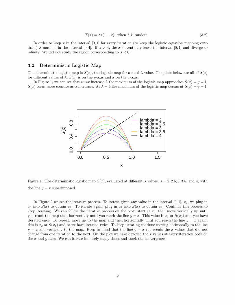
The deterministic logistic map is S(x), the logistic map for a fixed λ value. The plots below are all of S(x)for different values of λ; S(x) is on the y-axis and x on the x-axis.

In Figure 1, we can see that as we increase λ the maximum of the logistic map approaches S(x) = y = 1;S(x) turns more concave as λ increases. At λ = 4 the maximum of the logistic map occurs at S(x) = y = 1.

0.0 0.5 1.0 1.5

0.0

0.4

0.8

x

S(x

)

lambda = 2lambda = 2.5lambda = 3lambda = 3.5lambda = 4

Figure 1: The deterministic logistic map S(x), evaluated at different λ values, λ = 2, 2.5, 3, 3.5, and 4, with

the line y = x superimposed.

In Figure 2 we see the iterative process. To iterate given any value in the interval [0, 1], x0, we plug inx0 into S(x) to obtain x1. To iterate again, plug in x1 into S(x) to obtain x2. Continue this process tokeep iterating. We can follow the iterative process on the plot: start at x0, then move vertically up untilyou reach the map then horizontally until you reach the line y = x. This value is x1 or S(x0) and you haveiterated once. To repeat, move up to the map and then horizontally until you reach the line y = x again,this is x2 or S(x1) and so we have iterated twice. To keep iterating continue moving horizontally to the liney = x and vertically to the map. Keep in mind that the line y = x represents the x values that did notchange from one iteration to the next. On the plot we have denoted the x values at every iteration both onthe x and y axes. We can iterate infinitely many times and track the convergence.

2

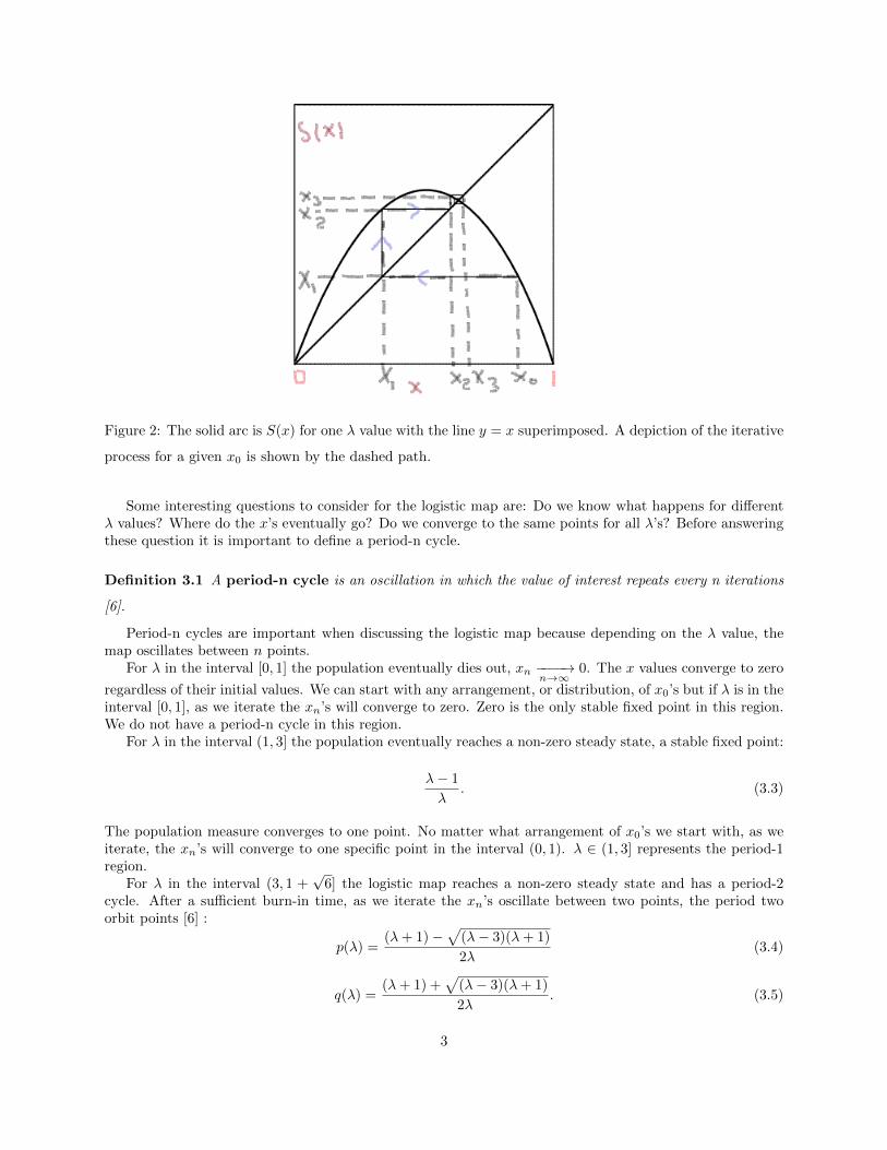
Figure 2: The solid arc is S(x) for one λ value with the line y = x superimposed. A depiction of the iterative

process for a given x0 is shown by the dashed path.

Some interesting questions to consider for the logistic map are: Do we know what happens for differentλ values? Where do the x’s eventually go? Do we converge to the same points for all λ’s? Before answeringthese question it is important to define a period-n cycle.

Definition 3.1 A period-n cycle is an oscillation in which the value of interest repeats every n iterations

[6].

Period-n cycles are important when discussing the logistic map because depending on the λ value, themap oscillates between n points.

For λ in the interval [0, 1] the population eventually dies out, xn −−−−→n→∞

0. The x values converge to zero

regardless of their initial values. We can start with any arrangement, or distribution, of x0’s but if λ is in theinterval [0, 1], as we iterate the xn’s will converge to zero. Zero is the only stable fixed point in this region.We do not have a period-n cycle in this region.

For λ in the interval (1, 3] the population eventually reaches a non-zero steady state, a stable fixed point:

λ− 1

λ. (3.3)

The population measure converges to one point. No matter what arrangement of x0’s we start with, as weiterate, the xn’s will converge to one specific point in the interval (0, 1). λ ∈ (1, 3] represents the period-1region.

For λ in the interval (3, 1 +√

6] the logistic map reaches a non-zero steady state and has a period-2cycle. After a sufficient burn-in time, as we iterate the xn’s oscillate between two points, the period twoorbit points [6] :

p(λ) =(λ+ 1)−

√(λ− 3)(λ+ 1)

2λ(3.4)

q(λ) =(λ+ 1) +

√(λ− 3)(λ+ 1)

2λ. (3.5)

3

Note the average of the period two orbits is: λ+12λ . If we stop iterating after n iterations, where n is sufficiently

large and the map has converged, the xn’s will be at one point mass. If we iterate one more time - arriveat the n + 1 iteration - the population measure is at a different point from the nth iteration, but a singlepoint nonetheless. In the n+ 2 iteration the population measure is at exactly the same point as in the nthiteration. In the n+3 iteration the population measure is at exactly the same point as in the n+1 iteration.This continues as we increase n, hence, the population measure oscillates between two points. λ ∈ (3, 1+

√6]

represents the period-2 region.For λ in the interval (1+

√6, 3.54409] (approximately) the logistic map has a period-4 cycle; the population

oscillates between 4 values. After sufficient burn-in time, if we inspect a vector of the last 8 iterations wewill note that the 1st and 5th entries are identical. Similarly, the following entry pairs will also be equal:2nd and 6th, 3rd and 7th, 4th and 8th. The population measure bounces between four different points inthe same consecutive order as we iterate. λ ∈ (1 +

√6, 3.54409] represents the period-4 region.

Period doublings occur as λ increases towards 3.56995 to cycles of period 8, 16, 32 and so on. However,as the period increases, the respective λ interval narrows. At approximately 3.56995 chaos ensues, so forλ ≥ 3.56995 the deterministic logistic map may exhibit chaotic behavior [6].

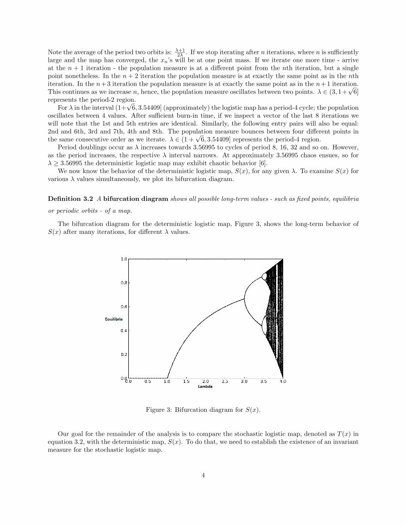
We now know the behavior of the deterministic logistic map, S(x), for any given λ. To examine S(x) forvarious λ values simultaneously, we plot its bifurcation diagram.

Definition 3.2 A bifurcation diagram shows all possible long-term values - such as fixed points, equilibria

or periodic orbits - of a map.

The bifurcation diagram for the deterministic logistic map, Figure 3, shows the long-term behavior ofS(x) after many iterations, for different λ values.

Figure 3: Bifurcation diagram for S(x).

Our goal for the remainder of the analysis is to compare the stochastic logistic map, denoted as T (x) inequation 3.2, with the deterministic map, S(x). To do that, we need to establish the existence of an invariantmeasure for the stochastic logistic map.

4

4 Unique Stable Invariant Density

In this section we will define a unique stable invariant density. First and foremost, we define density.

Definition 4.1 A density , fX(x), communicates all possible values of a random variable, X, and the

corresponding respective probabilities such that

Pr[a ≤ X ≤ b] =

∫ b

a

fX(x)dx.

In order to define invariant within the context of the logistic map, we will introduce the Frobenius-Perron Operator [3] for the logistic map. Once we have a definition for invariant we will go on to definestable density, unique density and unique stable invariant density.

4.1 The Frobenius-Perron Operator for the Logistic Map

The Frobenius-Perron Operator is useful for examining the evolution of densities [3] . We will follow thenotation utilized by Fisher and Radunskaya in [2] and a similar process to finding the Frobenius-PerronOperator as Lasota and Mackey in [3].

For the logistic map, we have the following notation.Let D denote the set of all probability densities supported on Ω = (0, 1), and let f(y) be an element in D.Let g(λ) denote the density of the λ’s, here g is uniform:

g(λ) =

1b−a in [a, b]

0 else,where a < b ∈ [0, 4].

The map T (x), equation 3.2, induces a map on f ∈ D given by the Frobenius-Perron operator, P . For thestochastic logistic map, T (x),

P f(x) =

∫ b

a

f(y)g(λ) dλ.

Let λ = xy(1−y) . Then,

P f(x) =

∫f(y)g

(x

y(1− y)

)dx

y(1− y). (4.1)

In order to find the bounds of integration, we have to integrate over the area in Figure 4. Because wedid a change of variables, we must integrate horizontally with regards to x.

5

Figure 4: T (x) for two iterations: T (x;λ0 = a) and T (x;λ1 = b) with the line y = x superimposed. In this

figure we illustrate how to integrate T (x) and how to find the bounds for equation 4.1.

When a ≤ λ ≤ b, x goes from b−√b2−4bx2b to b−

√b2−4bx2b or x goes from b−

√b2−4bx2b to a−

√a2−4ax2a and

from b+√b2−4bx2b to a+

√a2−4ax2a . This is because by(1 − y) = x ⇒ x = b±

√b2−4bx2b and ay(1 − y) = x ⇒ x =

a±√a2−4ax2a . Note: the max of λx(1− x) is at x = 1

2 and S( 12 ) = λ

4 .Thus, the Frobenius-Perron Operator for the logistic map with λ ∈ [a, b] is:

P f(x) =

0 b4 < x ≤ 1∫ b+

√b2−4bx2b

b−√

b2−4bx2b

1b−a

f(y)y(1−y)dy

a4 ≤ x ≤

b4

∫ a−√

a2−4ax2a

b−√

b2−4bx2b

1b−a

f(y)y(1−y)dy +

∫ b+√

b2−4bx2b

a+√

a2−4ax2a

1b−a

f(y)y(1−y)dy 0 ≤ x < a

4 .

Now that we know the Frobenius-Perron Operator for T (x) with uniform λ, we can define the following.

Definition 4.2 An invariant density is a density function, f∗, such that, P f∗ = f∗.

Note:

fn+1 = P fn(x) =

0 b4 < x ≤ 1∫ b+

√b2−4bx2b

b−√

b2−4bx2b

1b−a

fn(y)y(1−y)dy

a4 ≤ x ≤

b4

∫ a−√

a2−4ax2a

b−√

b2−4bx2b

1b−a

fn(y)y(1−y)dy +

∫ b+√

b2−4bx2b

a+√

a2−4ax2a

1b−a

fn(y)y(1−y)dy 0 ≤ x < a

4 .

6

Definition 4.3 A stable density is a density which is approached from some initial distribution, f0. That

is, f∗ is stable if limn→∞ fn+1 = limn→∞ P fn = f∗.

Definition 4.4 A unique density is a density that is the only invariant density.

Definition 4.5 A unique stable invariant density is a single density approached from any initial dis-

tribution, f0.

Note that the Frobenius-Perron Operator above is defined for the logistic map with λ ∼ U [a, b]. Wecan therefore create a Frobenius-Perron Operator for the whole period one region - or any other allowableregion. The Frobenius-Perron Operator allows us to check if a distribution is invariant or not. If f∗, is aunique stable distribution for the stochastic logistic map, T (x), with λ uniformly distributed on [a, b], andif when the Frobenius-Perron Operator is applied to f∗ we stay at f∗, then f∗ is also invariant. However,if we apply the Frobenius-Perron Operator to any f0 and converge to a different distribution f , then theexistence of the integral for one iteration does not say anything about the convergence of a particular f0 tof∗. The Frobenius-Perron Operator is therefore just a tool for analytically writing down f∗.

We know that a unique invariant density exists for the stochastic logistic map because of theorem 4.6 [1,p. 343].

Theorem 4.6 Assume that the distribution g of λn has a nonzero absolutely continuous component (with

respect to the Lebesgue measure on (0, 4)), whose density is bounded away from zero on some nondegenerate

interval in (1, 4). Assume

E[logλ1] > 0 and E[|log(4− λ1)|] <∞.

Then (a) the Markov process xn(n ≥ 0), defined recursively by x0, xn+1 = αn+1xn(1− xn) (n ≥ 0) where x0

takes values in (0, 1) and is independent of g, has a unique invariant probability π on (0, 1), and

1

N

N∑n=1

p(n)(x, dy)→ π(dy) in total variation distance, as N →∞

where pn is a one-step transition probability matrix on (0, 1) and (b) if, in addition, the density component

is bounded away from zero on an interval that includes an attractive periodic point of prime period m, then

pmk(x, dy)→ π(dy) in total variation distance, as k →∞.

In our logistic map setting, g is the uniform distribution on [a, b] s.t. 1 < a < b ≤ 4 hence, g has anonzero absolutely continuous component whose density is bounded away from zero on some nondegenerateinterval (1, 4). Furthermore,

7

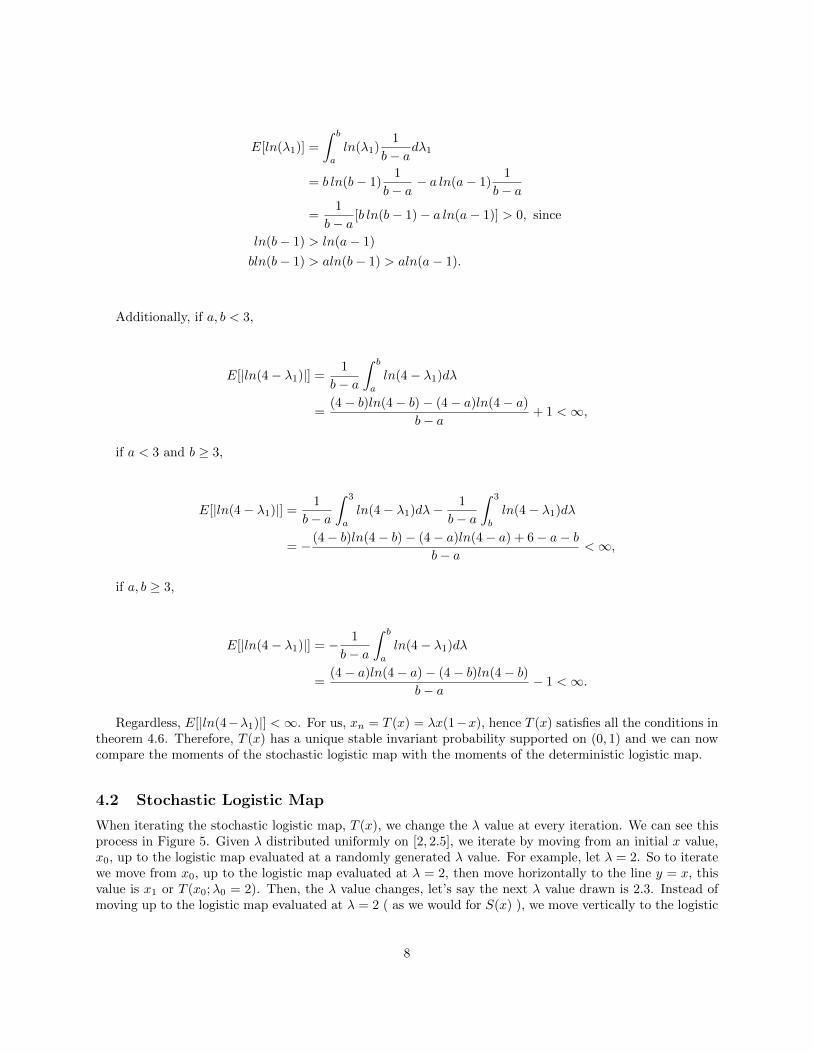
E[ln(λ1)] =

∫ b

a

ln(λ1)1

b− adλ1

= b ln(b− 1)1

b− a− a ln(a− 1)

1

b− a

=1

b− a[b ln(b− 1)− a ln(a− 1)] > 0, since

ln(b− 1) > ln(a− 1)

bln(b− 1) > aln(b− 1) > aln(a− 1).

Additionally, if a, b < 3,

E[|ln(4− λ1)|] =1

b− a

∫ b

a

ln(4− λ1)dλ

=(4− b)ln(4− b)− (4− a)ln(4− a)

b− a+ 1 <∞,

if a < 3 and b ≥ 3,

E[|ln(4− λ1)|] =1

b− a

∫ 3

a

ln(4− λ1)dλ− 1

b− a

∫ 3

b

ln(4− λ1)dλ

= − (4− b)ln(4− b)− (4− a)ln(4− a) + 6− a− bb− a

<∞,

if a, b ≥ 3,

E[|ln(4− λ1)|] = − 1

b− a

∫ b

a

ln(4− λ1)dλ

=(4− a)ln(4− a)− (4− b)ln(4− b)

b− a− 1 <∞.

Regardless, E[|ln(4−λ1)|] <∞. For us, xn = T (x) = λx(1−x), hence T (x) satisfies all the conditions intheorem 4.6. Therefore, T (x) has a unique stable invariant probability supported on (0, 1) and we can nowcompare the moments of the stochastic logistic map with the moments of the deterministic logistic map.

4.2 Stochastic Logistic Map

When iterating the stochastic logistic map, T (x), we change the λ value at every iteration. We can see thisprocess in Figure 5. Given λ distributed uniformly on [2, 2.5], we iterate by moving from an initial x value,x0, up to the logistic map evaluated at a randomly generated λ value. For example, let λ = 2. So to iteratewe move from x0, up to the logistic map evaluated at λ = 2, then move horizontally to the line y = x, thisvalue is x1 or T (x0;λ0 = 2). Then, the λ value changes, let’s say the next λ value drawn is 2.3. Instead ofmoving up to the logistic map evaluated at λ = 2 ( as we would for S(x) ), we move vertically to the logistic

8

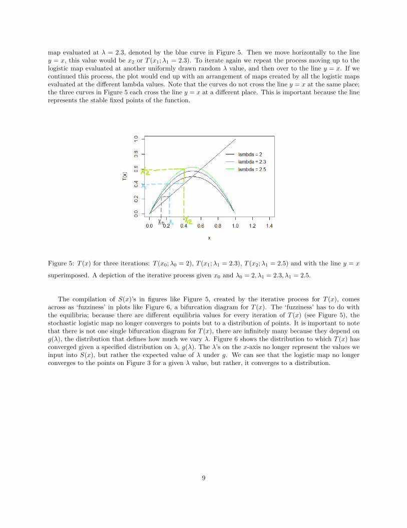
map evaluated at λ = 2.3, denoted by the blue curve in Figure 5. Then we move horizontally to the liney = x, this value would be x2 or T (x1;λ1 = 2.3). To iterate again we repeat the process moving up to thelogistic map evaluated at another uniformly drawn random λ value, and then over to the line y = x. If wecontinued this process, the plot would end up with an arrangement of maps created by all the logistic mapsevaluated at the different lambda values. Note that the curves do not cross the line y = x at the same place;the three curves in Figure 5 each cross the line y = x at a different place. This is important because the linerepresents the stable fixed points of the function.

Figure 5: T (x) for three iterations: T (x0;λ0 = 2), T (x1;λ1 = 2.3), T (x2;λ1 = 2.5) and with the line y = x

superimposed. A depiction of the iterative process given x0 and λ0 = 2, λ1 = 2.3, λ1 = 2.5.

The compilation of S(x)’s in figures like Figure 5, created by the iterative process for T (x), comesacross as ‘fuzziness’ in plots like Figure 6, a bifurcation diagram for T (x). The ‘fuzziness’ has to do withthe equilibria; because there are different equilibria values for every iteration of T (x) (see Figure 5), thestochastic logistic map no longer converges to points but to a distribution of points. It is important to notethat there is not one single bifurcation diagram for T (x), there are infinitely many because they depend ong(λ), the distribution that defines how much we vary λ. Figure 6 shows the distribution to which T (x) hasconverged given a specified distribution on λ, g(λ). The λ’s on the x-axis no longer represent the values weinput into S(x), but rather the expected value of λ under g. We can see that the logistic map no longerconverges to the points on Figure 3 for a given λ value, but rather, it converges to a distribution.

9

0.5 1.0 1.5 2.0 2.5 3.0 3.5 4.0

0.0

0.4

0.8

lambda

x

Figure 6: A bifurcation diagram for T (x) with g(λ) = 10.2 for λ ∈ [a − .1, a + .1] and a as the x coordinate

on the plot. Note the x-axis of this figure is for 0.5 ≤ a ≤ 3.9 but we can plot a bifurcation diagram for

a ∈ [0, 4].

For every λ value on the x-axis of Figure 6, there is vertical distribution of x values that T (x) approachesas we iterate. Recall that a bifurcation diagram tells us the long-term behavior of a map. Outside the chaoticregion, the bifurcation diagram for S(x) shows that S(x) converges to points. The bifurcation diagrams forT (x) show that T (x) converges to a distribution at each λ. Recall in section 4.1 we demonstrated that thisdistribution was a unique stable invariant distribution, for given uniform g(λ)’s.

4.3 Simulations

The simulation results agree with the theory that the parameters converge in the period one, two and fourregions; that a unique stable invariant density exists for those regions.

Figure 7 is a slice of a bifurcation diagram of T (x) ( as in Figure 6) in the period one region. Particularly,it is a vertical slice of a bifurcation diagram of T (x)with λ ∼ U [1.484, 1.532]. Figure 7 shows the distributionof the x values as we iterate. If we start with 1000 uniformly drawn random x0’s, so with f as the uniformdistribution on [0, 1] indicated by the purple curve in Figure 7, and iterate 1 time, the x values are distributedby the blue curve. After 10 iterations the x-values are distributed by the green curve and after 50 iterationsdistributed by the yellow curve, which lies below the final density in Figure 7. This is because the yellow curveis covered up by the orange curve (the distribution of x-values after 100 iterations ), which in turn is coveredup by the red curve (the distribution of x-values after 10000 iterations ). We expect that the red distributionis the unique stable invariant distribution for the stochastic logistic map with λ ∼ U [1.484, 1.532]. Recall f∗

is the unique stable invariant distribution, and hence once the x-values are distributed by f∗ they will staydistributed by f∗ indefinitely, regardless of how many more times we iterate.

10

0.30 0.35 0.40 0.45

05

1015

20

Iterations for Period 1 (lambda =1.508)

x

Den

sity

x0x1x10x50x100x10000

Figure 7: Shows the distribution of the x’s for the initial distribution, the 1st, 10th, 50th, 100th, and

10000th iterations in purple, blue, green, yellow, orange, and red respectively for λ = 1.508. If you apply the

Frobenius-Perron Operator to the red distribution we expect that you would get the red distribution back;

hence we believe the red distribution to be invariant.

Similarly, Figure 8 is a slice of a bifurcation diagram for T (x) with λ ∼ U [3.184, 3.232]. The figure hastwo humps instead of one because the bifurcation diagram for T (x), like S(x), has two branches in the periodtwo region; each hump represents the vertical distribution of the x’s in one branch. Again, we started withf as the uniform distribution on [0, 1], denoted by the purple curve in Figure 8. After one iteration the x’sare distributed by the blue curve. After 10 iterations by the green curve. After 50 iterations by the yellowcurve. After 100 iterations by the orange curve which is covered by the red curve, the distribution of the x’safter 10000 iterations. Although it took more iterations to converge than in the period one region, we stillsee that the distribution of x’s is converging. Again, we expect that the red distribution is the unique stableinvariant distribution for the stochastic logistic map, T (x), with λ ∼ U [3.184, 3.232].

0.4 0.5 0.6 0.7 0.8 0.9

05

1015

Iterations for Period 2 (lambda =3.208)

x

Den

sity

x0x1x10x50x100x10000

Figure 8: Shows the distribution of the x’s for the initial distribution, the 1st, 10th, 50th, 100th, and 10000th

iterations in purple, blue, green, yellow, orange, and red respectively for λ = 3.208.

Figure 7 supports the claim that if we start with f as the uniform distribution on [0, 1] and with λ ∼U [a, b]s.t.a, b ∈ (1, 3], the period one region, then we do indeed reach a stable invariant distribution. Similarly,

11

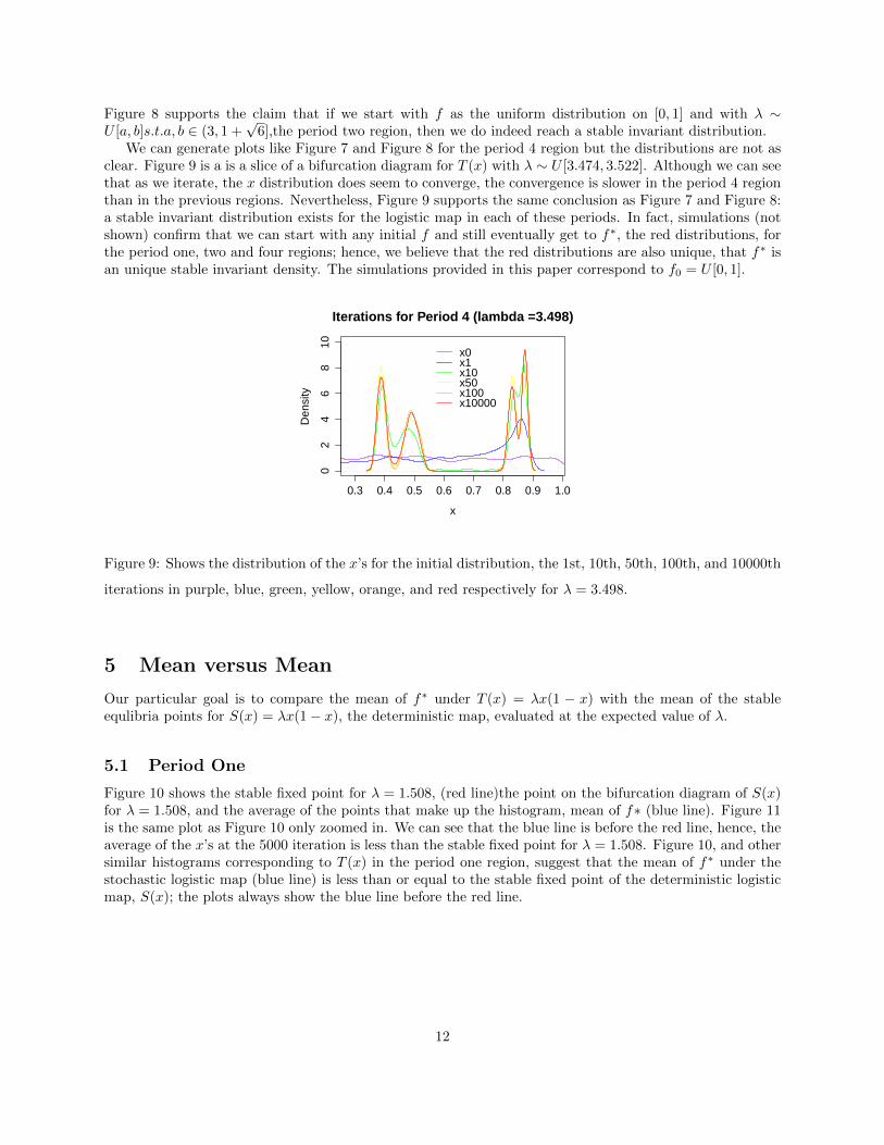
Figure 8 supports the claim that if we start with f as the uniform distribution on [0, 1] and with λ ∼U [a, b]s.t.a, b ∈ (3, 1 +

√6],the period two region, then we do indeed reach a stable invariant distribution.

We can generate plots like Figure 7 and Figure 8 for the period 4 region but the distributions are not asclear. Figure 9 is a is a slice of a bifurcation diagram for T (x) with λ ∼ U [3.474, 3.522]. Although we can seethat as we iterate, the x distribution does seem to converge, the convergence is slower in the period 4 regionthan in the previous regions. Nevertheless, Figure 9 supports the same conclusion as Figure 7 and Figure 8:a stable invariant distribution exists for the logistic map in each of these periods. In fact, simulations (notshown) confirm that we can start with any initial f and still eventually get to f∗, the red distributions, forthe period one, two and four regions; hence, we believe that the red distributions are also unique, that f∗ isan unique stable invariant density. The simulations provided in this paper correspond to f0 = U [0, 1].

0.3 0.4 0.5 0.6 0.7 0.8 0.9 1.0

02

46

810

Iterations for Period 4 (lambda =3.498)

x

Den

sity

x0x1x10x50x100x10000

Figure 9: Shows the distribution of the x’s for the initial distribution, the 1st, 10th, 50th, 100th, and 10000th

iterations in purple, blue, green, yellow, orange, and red respectively for λ = 3.498.

5 Mean versus Mean

Our particular goal is to compare the mean of f∗ under T (x) = λx(1 − x) with the mean of the stableequlibria points for S(x) = λx(1− x), the deterministic map, evaluated at the expected value of λ.

5.1 Period One

Figure 10 shows the stable fixed point for λ = 1.508, (red line)the point on the bifurcation diagram of S(x)for λ = 1.508, and the average of the points that make up the histogram, mean of f∗ (blue line). Figure 11is the same plot as Figure 10 only zoomed in. We can see that the blue line is before the red line, hence, theaverage of the x’s at the 5000 iteration is less than the stable fixed point for λ = 1.508. Figure 10, and othersimilar histograms corresponding to T (x) in the period one region, suggest that the mean of f∗ under thestochastic logistic map (blue line) is less than or equal to the stable fixed point of the deterministic logisticmap, S(x); the plots always show the blue line before the red line.

12

5,000 iteration for Lambda=1.508

x

Den

sity

0.330 0.335 0.340 0.3450

5010

015

0

Figure 10: Histogram of the 5000th iteration for T (x) with λ ∼ U [1.484, 1.532] and the relevant means.

5,000 iteration Lambda=1.508

x

Den

sity

0.3368 0.3370 0.3372 0.3374

050

100

150

mean of f*stable fixed pt forlambda = 1.508

Figure 11: Zoomed in version of figure 10

In fact, we know that the blue line will always come before the red line in the period one region becauseof the following theorem.

Theorem 5.1 In the period one region, λ ∈ (1, 3], the mean of f∗ under the stochastic logistic map is less

than or equal to the stable fixed point of the deterministic map at Eg(λ), where g is a continuous distribution

of λ .

Proof

Let f∗ be the unique invariant density of the logistic map and g be the distribution of λ. Then because

f∗ and g are independent,

Ef∗ [x] = E(f∗,g)[λx(1− x)] = Eg[λ]Ef∗ [x(1− x)] = Eg[λ](Ef∗ [x]− Ef∗ [x2]).

13

Let λ = Eg[λ]. So,

Ef∗ [x] = λ(Ef∗ [x]− Ef∗ [x2]) =⇒ λEf∗ [x2] = (λ− 1)Ef∗ [x],

and by Jensen’s inequality, Ef∗ [x2] ≥ (Ef∗ [x])2.

Hence,

λEf∗ [x2] = (λ− 1)Ef∗ [x] ≥ λ(Ef∗ [x])2

=⇒ (λ− 1) ≥ λEf∗ [x]

=⇒ λ− 1

λ≥ Ef∗ [x].

Where the fixed point of S(x) at λ is λ−1λ

and Ef∗ [x] is the expected value of T (x) under the unique stable

invariant distribution.

Note: the inequality in theorem 5.1 holds for λ in any region. However, the equilibria will be a different

function of λ (i.e., not λ−1λ ) as λ changes regions. That is, λ−1

λis the mean of f∗ only for the period one

region. Therefore, our proof does not tell us anything about the relationship between the stochastic anddeterministic means in other regions.

5.2 Period Two

Figure 12 shows a histogram of the 4999 : 5000th iterations - the last two iterations are included because λis in the period two region and the x’s oscillate between the two humps- for T (x) with λ ∼ U [3.184, 3.232]and the stochastic and deterministic means. The orange line on the histogram corresponds to the averageof the two bifurcation points for λ = 3.208, the points on the bifurcation diagram of S(x) for λ = 3.208.The green line depicts the average of the points that make up the histogram. In Figure 13, the zoomed inversion of Figure 12, we can see that the orange line is before the green line, so the average of the pointsthat make up the histogram is greater than the average of the two stable fixed points. Figure 12, and otherhistograms of the last two iterations of T (x) for λ in the period two region, suggest that the expected valueof f∗ under the stochastic logistic map is greater than or equal to the mean of the stable fixed points ofthe deterministic map for Eg(λ), where g is the distribution of the λ’s. That is, the relationship between thestochastic and deterministic means in the period two region is the opposite of the relationship in the periodone region.

14

4,999 & 5,000 iteration Lambda=3.2

xD

ensi

ty0.50 0.60 0.70 0.80

010

3050

mean of respectivehump under f*stable fixed pts forlambda = 3.2mean of f*mean of stablefixed points

Figure 12: A histogram of the 4999 : 5000th iterations - the last two iterations are included because λ is in

the period two region and the x’s oscillate between the two humps- for T (x) with λ ∼ U [3.184, 3.232] and

the stochastic and deterministic means.

4,999 & 5,000 iteration Lambda=3.2

x

Den

sity

0.6560 0.6565 0.6570 0.6575

010

3050 mean of f*

mean of stablefixed points

Figure 13: Zoomed in version of figure 12.

Conjecture 5.2 In the period two region, λ ∈ (3, 1 +√

6], the expected value of f∗ under the stochastic

logistic map is greater than or equal to the average of the stable fixed points of the deterministic map at

Eg(λ), when g is a continuous symmetric distribution of λ.

Not only do the simulations support conjecture 5.2, but we also believe the conjecture to be true becauseof the convexity of the logistic map. The map has higher convexity at p(λ) than at q(λ) (see equation 3.4and equation 3.5). If we can prove that Jensen’s inequality is “stronger” for p(λ) than for q(λ), then we canprove conjecture 5.2.

Though it does not gives us the true expected value of f∗ (the stochastic mean), we can show that theexpected value of the average of the bifurcation points is larger than the deterministic mean. Our workdemonstrates that the convexity of p and q lead to higher values in expected value than simply the averageat the expected value of λ. In turn, we have some evidence that conjecture 5.2 is true.

15

Then conjecture 5.2 follows,Let h(λ) = p(λ) + q(λ) where p(λ) and q(λ) are the two stable fixed points for the period two regions,

then we have:

h(λ) = 1 +1

λ⇒ h′(λ) = − 1

λ2⇒ h′′(λ) =

2

λ3> 0.

Therefore, by Jensen’s inequality:

E[p(λ) + q(λ)] = E[h(λ)] > h(E[λ]) = p(E[λ]) + q(E[λ]),

E[p(λ) + q(λ)]

2≥ p(E[λ]) + q(E[λ])

2E[p(λ) + q(λ)]

2≥ deterministic mean.

The problem arises with how we are defining “mean”. It is not true that the mean of x is the same as themean of the fixed points, since, at each iteration, the x-value will move toward the fixed point correspondingto whatever λ-value was picked but it doesn’t jump right to it; the x-values move towards the period-twopoints of the new λ but they do not jump there. We believe that the convexity plays a vital role because asλ increases the p(λ) decreases, on average, more than q(λ) increases.

5.3 Period Four

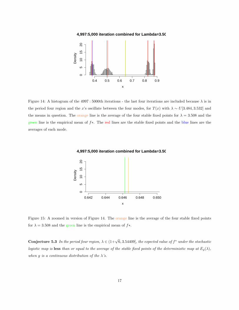
Figure 14 shows the average of the four stable fixed points for λ = 3.508, the points on the bifurcationdiagram of S(x) for λ = 3.508, and the average of the points that make up the histogram. In Figure 15, thezoomed in version of Figure 14, we can see that the green line is before the orange line, so the average of thepoints that make up the histogram (which is approximately f∗) is less than the average of the four stablefixed points, just as in the period one region. Figure 14, and other histograms of the last four iterations ofT (x) for λ in the period four region, suggest that the expected value of f∗ under the stochastic logistic mapis less than or equal to the mean of the stable fixed points of the deterministic map for Eg(λ), where g isthe continuous distribution of the λ’s, because the green line will come before the orange line.

16

4,997:5,000 iteration combined for Lambda=3.508

x

Den

sity

0.4 0.5 0.6 0.7 0.8 0.90

510

1520

Figure 14: A histogram of the 4997 : 5000th iterations - the last four iterations are included because λ is in

the period four region and the x’s oscillate between the four modes, for T (x) with λ ∼ U [3.484, 3.532] and

the means in question. The orange line is the average of the four stable fixed points for λ = 3.508 and the

green line is the empirical mean of f∗. The red lines are the stable fixed points and the blue lines are the

averages of each mode.

4,997:5,000 iteration combined for Lambda=3.508

x

Den

sity

0.642 0.644 0.646 0.648 0.650

05

1015

20

Figure 15: A zoomed in version of Figure 14. The orange line is the average of the four stable fixed points

for λ = 3.508 and the green line is the empirical mean of f∗.

Conjecture 5.3 In the period four region, λ ∈ (1+√

6, 3.54409], the expected value of f∗ under the stochastic

logistic map is less than or equal to the average of the stable fixed points of the deterministic map at Eg(λ),

when g is a continuous distribution of the λ’s.

17

5.4 Comparison of Means in the Grand Scheme

Figure 10, Figure 12, and Figure 14 allow us to examine the expected value of f∗ under T (x) and the averageof the stable fixed points of S(x) for three particular values of λ. We want to be able to compare the averagesof the stochastic and deterministic logistic maps for a variety of λ’s at the same time, instead of one at atime. We can do that by looking at plots like Figure 16.The x-axis of Figure 16 corresponds to the Eg(λ),

when g(λ) =

1b−a in [a, b]

0 elsewith a, b ∈ [0, 4] and b− a = 0.048. A vertical slice of Figure 16 in the period

one, two and four regions corresponds to the vertical lines drawn on the histograms in plots like Figure 10,Figure 12 and Figure 14. The lines on the histograms in Figure 10, Figure 12 and Figure 14 are rotated 90degrees counter-clockwise and consolidated into one dimension to make up a vertical slice of Figure 16.

1.0 1.5 2.0 2.5 3.0 3.5 4.0

0.0

0.4

0.8

lambda

x

Figure 16: The stable fixed points (red), the averages of the stable fixed points (red in the period 1 region,

orange in the period 2 and 4 regions), the average of each mode of f∗ (blue), and the mean of f∗ (blue in

the period 1 region, green in the period 2 and 4 regions) are depicted in the plot.

In order to examine the two conjectures included in this paper, we will zoom in on the period twoand period four regions of Figure 16; we omit period one because we have proven the inequality of themeans for that region. It is important to note that the orange and green lines in Figure 16 move closerand farther together depending on the width of the interval for [a, b] where a and b are defined within

g(λ) =

1b−a in [a, b]

0 elsewith a, b ∈ [0, 4] and b − a = 0.048. Intuitively this makes sense because as the

interval [a, b] narrows, T (x) is less random and T (x) approaches S(x).

18

5.4.1 Period Two

3.0 3.1 3.2 3.3 3.4

0.4

0.6

0.8

period 2

lambda

x

Figure 17: Figure 16 zoomed in on the period 2 region. The stable fixed points are red, the average of the

stable fixed points is orange, the averages of each hump are blue, and the mean of f∗ is green. Note that

the green lines lie entirely above the orange line.

3.0 3.1 3.2 3.3 3.4 3.5

0.64

00.

655

0.67

0

period 2 comparison of means

lambda

x

Figure 18: Figure 16 zoomed in on the average of the stable fixed points (orange) and the mean of f∗ (green)

for the period 2 region.

In Figure 17 the red lines are the two stable fixed points of S(x) and hence, are the exact same lines asthe lines in Figure 3, the bifurcation diagram of S(x), in the period two region. The blue lines represent

19

the averages of the points in each mode of a histogram like Figure 12, for the corresponding Eg(λ) on thex-axis. Although the blue and red lines are informative, our interest lies on the orange and green lines. Wewant the orange line, the average of the two stable fixed points of S(x), to be entirely below the green line,the mean of f∗ under T (x), for the entire period two region. When we zoom in on the orange and greenlines, as in Figure 18, we can see that indeed the orange line is below the green line for λ ∼ U [a, b] such thata, b ∈ (3, 1 +

√6] (or for λdistributed symmetrically with endpoints in the period 2 region). In Figure 18

we see that near the endpoints the lines switch directions, that is because near the value 3, the distributionof λ is uniform on [a, b] with a in the period one region and b in the period two region and near 1 +

√6,

the distribution of λ is uniform on [a, b] with a in the period two region and b in the period four region.However, if we let λ range solely in the period 2 region, then the green line is above the orange line. Hence,our simulations support our period two conjecture.

5.4.2 Period Four

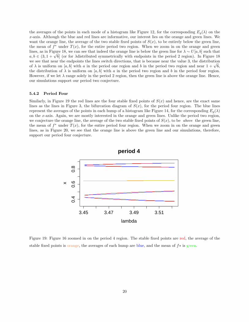
Similarly, in Figure 19 the red lines are the four stable fixed points of S(x) and hence, are the exact samelines as the lines in Figure 3, the bifurcation diagram of S(x), for the period four region. The blue linesrepresent the averages of the points in each hump of a histogram like Figure 14, for the corresponding Eg(λ)on the x-axis. Again, we are mostly interested in the orange and green lines. Unlike the period two region,we conjecture the orange line, the average of the two stable fixed points of S(x), to be above the green line,the mean of f∗ under T (x), for the entire period four region. When we zoom in on the orange and greenlines, as in Figure 20, we see that the orange line is above the green line and our simulations, therefore,support our period four conjecture.

3.45 3.47 3.49 3.51

0.4

0.6

0.8

period 4

lambda

x

Figure 19: Figure 16 zoomed in on the period 4 region. The stable fixed points are red, the average of the

stable fixed points is orange, the averages of each hump are blue, and the mean of f∗ is green.

20

3.45 3.47 3.49 3.51

0.64

00.

644

0.64

8

period 4 comparison of means

lambda

x

Figure 20: Figure 16 zoomed in on the average of the stable fixed points (orange) and the mean of f∗ (green)

for the period 4 region.

6 Conclusion

Our goal was to compare the expected value of the deterministic and stochastic logistic map in differentperiods. In order to talk about the expected value of the stochastic logistic map, a unique stable invariantdensity needs to exist for T (x). Our simulations for the period 1, 2, and 4 regions support the existence ofa unique stable invariant density, and we provide a proof that a unique stable invariant density exists forthe logistic map. Hence, we can compare the expected value of S(x) with the mean of f∗ under T (x). Inthe period one region, the fixed point - average of the deterministic map - is greater than or equal to theexpected value of the xs under the unique stable invariant distribution - the long term average of T (x). Interms of a growth model, if something in the environment is randomly fluctuating, affecting the birthratesof a population, then the average population will be smaller. For the period 2 region we conjecture thatthe average of the fixed points for the period 2 region for the deterministic map is less than or equal to theaverage under the unique stable invariant distribution of T (x). In a growth model, the average populationwill be greater when the environment is randomly fluctuating. In the period 4 region our simulations supportthe conjecture that the direction of the inequality switches back - the average of the fixed points for theperiod 2 region for the deterministic map is greater than or equal to the average under the unique stableinvariant distribution of T (x). In the period one and four regions the stochasticity is detrimental, but inthe period two region it is evolutionary advantageous. It makes sense to conjecture that as we increase theperiod, the direction of the inequality switches back and forth, at least through the period doubling rangeof λ.

References

[1] Rabu Bhattacharya and Mukul Majumbar. Random Dynamical Systems: Theory and Applications.Cambridge University Press, Cambridge, 2007.

21

[2] Leigh Fisher and Ami Radunskaya. Ergodicity,loss of capacity and first passage times in a stochasticgrowth model. 2012.

[3] Andrzej Lasota and Michael C. Mackey. Chaos, fractals, and noise: stochastic aspects of dynamics.Springer-Verlag, New York, 1994.

[4] Robert M. May. Simple mathematical models with very complicated dynamics. Nature, 261:459–467,1976.

[5] Larry L. Rockwood. Introduction to Population Ecology. Blackwell Pub, Malden, MA, 2006.

[6] Steven H. Strogatz. Nonliniear Dynamics and Chaos: With Applications to Physics, Biology, Chemistry,and Engineering. Addison-Wesley Pub., Reading, MA, 1994.

22