LONESTARTM H2S Scavenger Analyzer Rapid, At-Line Analysis of H2S Scavenger and By-Products

in Crude Oil using LONESTARTM

Contact us

www.owlstonenanotech.com

2 | P a g e

Contents

Introduction .................................................................................................................................... 3

Features of Lonestar H2S Scavenger Analyzer ........................................................................... 3

The Benefits of Deploying Lonestar H2S Scavenger Analyzer ................................................... 3

The LONESTARTM Portable Analyzer ............................................................................................... 4

Instrumentation .............................................................................................................................. 5

Calibration ....................................................................................................................................... 6

Sample Preparation and Analysis ................................................................................................... 6

Method Validation .......................................................................................................................... 7

Sample to sample repeatability ................................................................................................. 7

Appendix A: FAIMS Technology at a Glance ................................................................................. 10

Sample preparation and introduction ..................................................................................... 10

Carrier Gas ................................................................................................................................ 11

Ionisation Source ...................................................................................................................... 11

Mobility .................................................................................................................................... 14

Detection and Identification .................................................................................................... 15

Appendix D Generating Calibration Standards with the OVG-4TM ............................................... 18

Adding Precision Humidity with the Owlstone OHG-4TM Humidity Generator ....................... 19

3 | P a g e

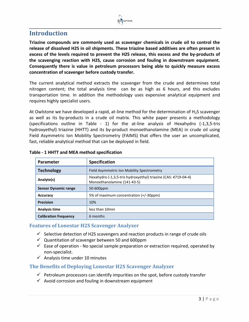
Introduction

Triazine compounds are commonly used as scavenger chemicals in crude oil to control the release of dissolved H2S in oil shipments. These triazine based additives are often present in excess of the levels required to prevent the H2S release, this excess and the by-products of the scavenging reaction with H2S, cause corrosion and fouling in downstream equipment. Consequently there is value in petroleum processors being able to quickly measure excess concentration of scavenger before custody transfer.

The current analytical method extracts the scavenger from the crude and determines total nitrogen content; the total analysis time can be as high as 6 hours, and this excludes transportation time. In addition the methodology uses expensive analytical equipment and requires highly specialist users.

At Owlstone we have developed a rapid, at-line method for the determination of H2S scavenger as well as its by-products in a crude oil matrix. This white paper presents a methodology (specifications outline in Table - 1) for the at-line analysis of Hexahydro (-1,3,5-tris hydroxyethyl) triazine (HHTT) and its by-product monoethanolamine (MEA) in crude oil using Field Asymmetric Ion Mobility Spectrometry (FAIMS) that offers the user an uncomplicated, fast, reliable analytical method that can be deployed in field.

Table - 1 HHTT and MEA method specification

Parameter Specification

Technology Field Asymmetric Ion Mobility Spectrometry

Analyte(s) Hexahydro (-1,3,5-tris hydroxyethyl) triazine (CAS: 4719-04-4) Monoethanolamine (141-43-5)

Sensor Dynamic range 50-600ppm

Accuracy 5% of maximum concentration (+/-30ppm)

Precision 10%

Analysis time less than 10min

Calibration frequency 6 months

Features of Lonestar H2S Scavenger Analyzer

Selective detection of H2S scavengers and reaction products in range of crude oils Quantitation of scavenger between 50 and 600ppm Ease of operation - No special sample preparation or extraction required, operated by

non-specialist. Analysis time under 10 minutes

The Benefits of Deploying Lonestar H2S Scavenger Analyzer

Petroleum processors can identify impurities on the spot, before custody transfer Avoid corrosion and fouling in downstream equipment

4 | P a g e

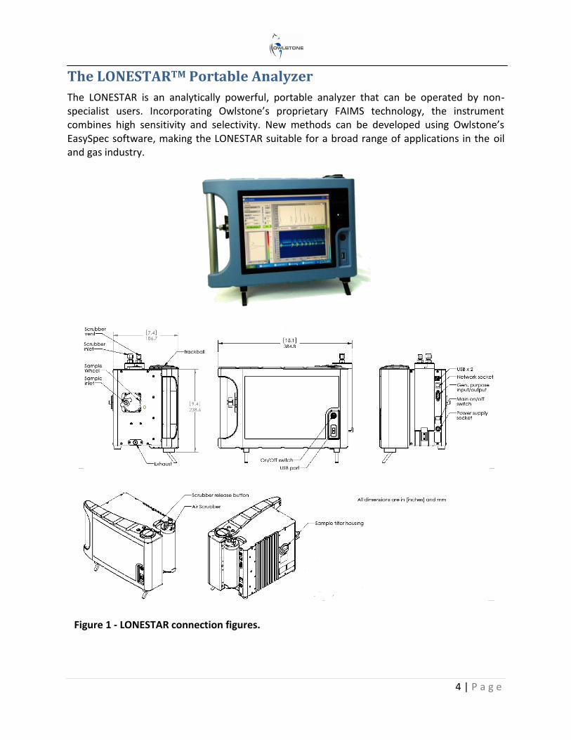
The LONESTARTM Portable Analyzer

The LONESTAR is an analytically powerful, portable analyzer that can be operated by non-specialist users. Incorporating Owlstone’s proprietary FAIMS technology, the instrument combines high sensitivity and selectivity. New methods can be developed using Owlstone’s EasySpec software, making the LONESTAR suitable for a broad range of applications in the oil and gas industry.

Figure 1 - LONESTAR connection figures.

5 | P a g e

Instrumentation

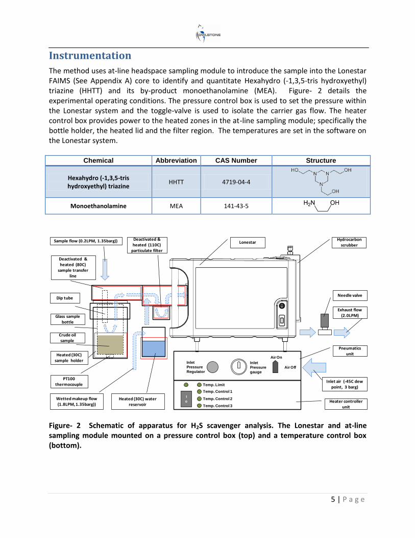
The method uses at-line headspace sampling module to introduce the sample into the Lonestar FAIMS (See Appendix A) core to identify and quantitate Hexahydro (-1,3,5-tris hydroxyethyl) triazine (HHTT) and its by-product monoethanolamine (MEA). Figure- 2 details the experimental operating conditions. The pressure control box is used to set the pressure within the Lonestar system and the toggle-valve is used to isolate the carrier gas flow. The heater control box provides power to the heated zones in the at-line sampling module; specifically the bottle holder, the heated lid and the filter region. The temperatures are set in the software on the Lonestar system.

Chemical Abbreviation CAS Number Structure

Hexahydro (-1,3,5-tris hydroxyethyl) triazine

HHTT 4719-04-4

Monoethanolamine MEA 141-43-5

Figure- 2 Schematic of apparatus for H2S scavenger analysis. The Lonestar and at-line sampling module mounted on a pressure control box (top) and a temperature control box (bottom).

Io

Temp. Limit

Temp. Control 1

Temp. Control 2

Temp. Control 3

Air On

Air Off

Inlet

Pressure

gauge

Inlet

Pressure

Regulator

Needle valve

Hydrocarbon scrubber

Heater controller unit

Pneumatics unit

Inlet air (-45C dew point, 3 barg)

Exhaust flow (2.0LPM)

LonestarSample flow (0.2LPM, 1.35barg)) Deactivated & heated (110C)

particulate filter

Deactivated & heated (80C)

sample transfer line

Crude oil sample

PT100 thermocouple

Heated (30C) sample holder

Dip tube

Wetted makeup flow (1.8LPM, 1.35barg))

Heated (30C) water reservoir

Glass sample bottle

6 | P a g e

Calibration

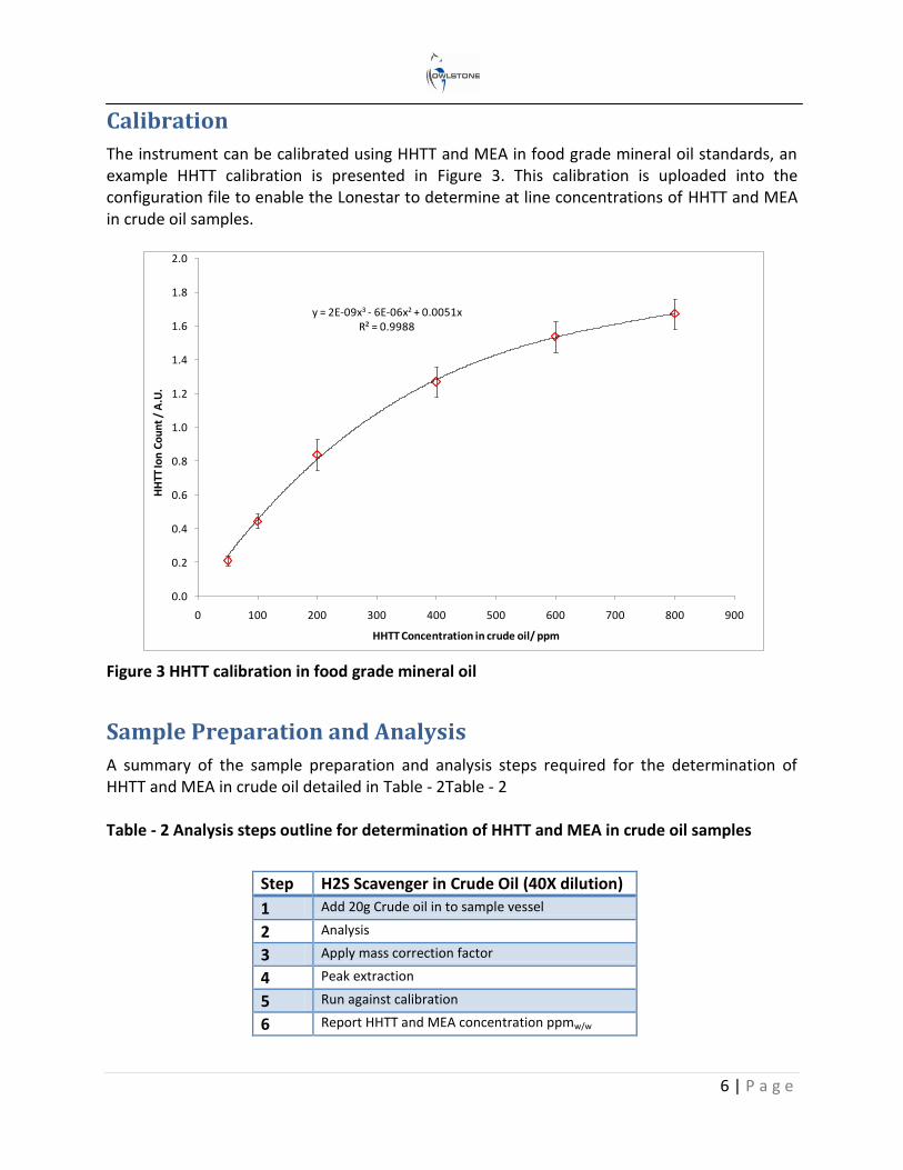
The instrument can be calibrated using HHTT and MEA in food grade mineral oil standards, an example HHTT calibration is presented in Figure 3. This calibration is uploaded into the configuration file to enable the Lonestar to determine at line concentrations of HHTT and MEA in crude oil samples.

Figure 3 HHTT calibration in food grade mineral oil

Sample Preparation and Analysis

A summary of the sample preparation and analysis steps required for the determination of HHTT and MEA in crude oil detailed in Table - 2Table - 2 Table - 2 Analysis steps outline for determination of HHTT and MEA in crude oil samples

Step H2S Scavenger in Crude Oil (40X dilution)

1 Add 20g Crude oil in to sample vessel

2 Analysis

3 Apply mass correction factor

4 Peak extraction

5 Run against calibration

6 Report HHTT and MEA concentration ppmw/w

y = 2E-09x3 - 6E-06x2 + 0.0051xR² = 0.9988

0.0

0.2

0.4

0.6

0.8

1.0

1.2

1.4

1.6

1.8

2.0

0 100 200 300 400 500 600 700 800 900

HH

TT Io

n C

ou

nt

/ A

.U.

HHTT Concentration in crude oil/ ppm

7 | P a g e

Method Validation

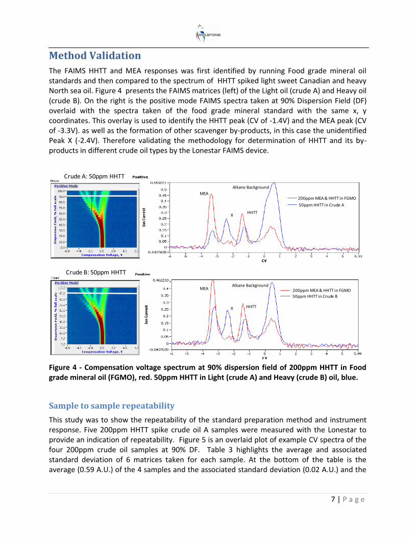
The FAIMS HHTT and MEA responses was first identified by running Food grade mineral oil standards and then compared to the spectrum of HHTT spiked light sweet Canadian and heavy North sea oil. Figure 4 presents the FAIMS matrices (left) of the Light oil (crude A) and Heavy oil (crude B). On the right is the positive mode FAIMS spectra taken at 90% Dispersion Field (DF) overlaid with the spectra taken of the food grade mineral standard with the same x, y coordinates. This overlay is used to identify the HHTT peak (CV of -1.4V) and the MEA peak (CV of -3.3V). as well as the formation of other scavenger by-products, in this case the unidentified Peak X (-2.4V). Therefore validating the methodology for determination of HHTT and its by-products in different crude oil types by the Lonestar FAIMS device.

Figure 4 - Compensation voltage spectrum at 90% dispersion field of 200ppm HHTT in Food grade mineral oil (FGMO), red. 50ppm HHTT in Light (crude A) and Heavy (crude B) oil, blue.

Sample to sample repeatability

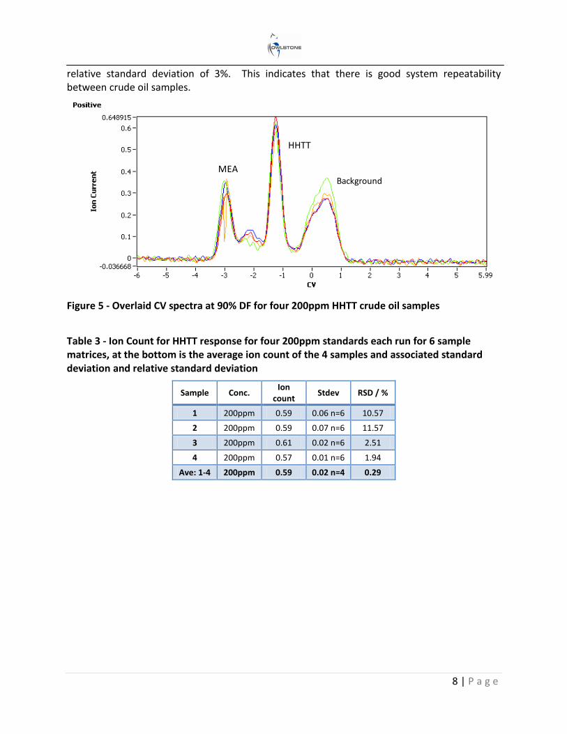
This study was to show the repeatability of the standard preparation method and instrument response. Five 200ppm HHTT spike crude oil A samples were measured with the Lonestar to provide an indication of repeatability. Figure 5 is an overlaid plot of example CV spectra of the four 200ppm crude oil samples at 90% DF. Table 3 highlights the average and associated standard deviation of 6 matrices taken for each sample. At the bottom of the table is the average (0.59 A.U.) of the 4 samples and the associated standard deviation (0.02 A.U.) and the

Crude B: 50ppm HHTT

Crude A: 50ppm HHTT

200ppm MEA & HHTT in FGMO

200ppm MEA & HHTT in FGMO

50ppm HHTT in Crude B

50ppm HHTT in Crude A

MEA

MEA

HHTT

HHTT

X

X

Alkane Background

Alkane Background

8 | P a g e

relative standard deviation of 3%. This indicates that there is good system repeatability between crude oil samples.

Figure 5 - Overlaid CV spectra at 90% DF for four 200ppm HHTT crude oil samples

Table 3 - Ion Count for HHTT response for four 200ppm standards each run for 6 sample matrices, at the bottom is the average ion count of the 4 samples and associated standard deviation and relative standard deviation

Sample Conc. Ion

count Stdev RSD / %

1 200ppm 0.59 0.06 n=6 10.57

2 200ppm 0.59 0.07 n=6 11.57

3 200ppm 0.61 0.02 n=6 2.51

4 200ppm 0.57 0.01 n=6 1.94

Ave: 1-4 200ppm 0.59 0.02 n=4 0.29

HHTT

MEABackground

9 | P a g e

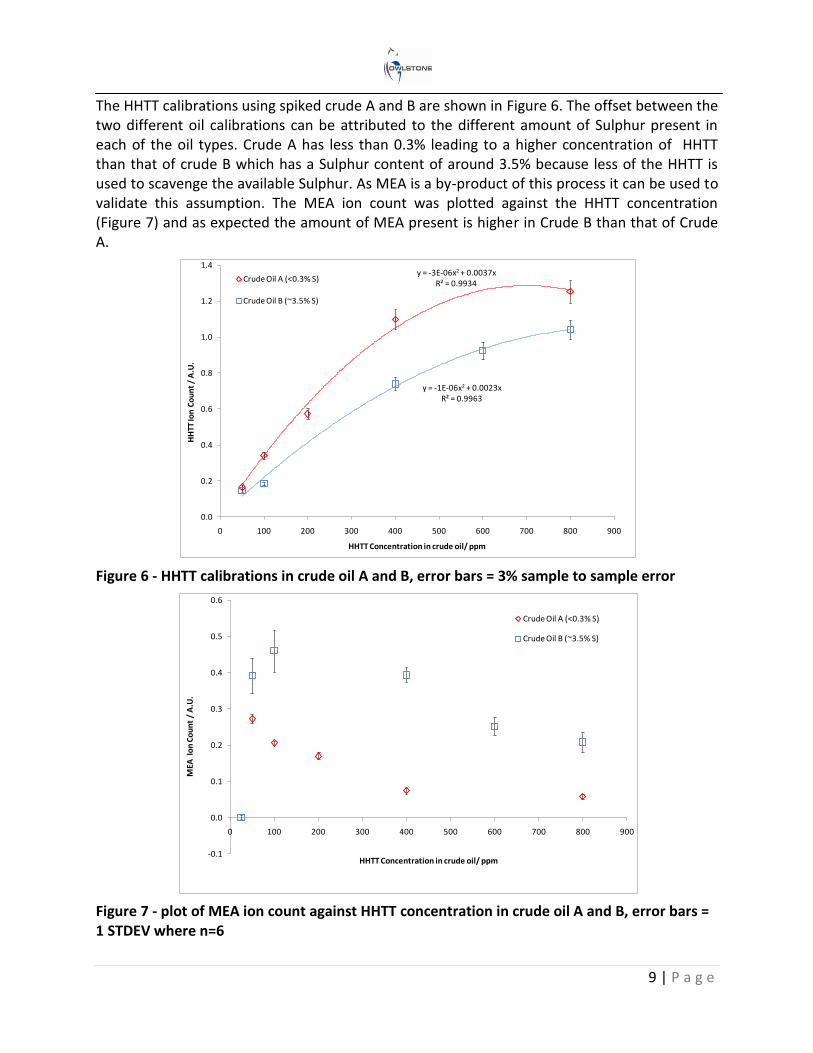
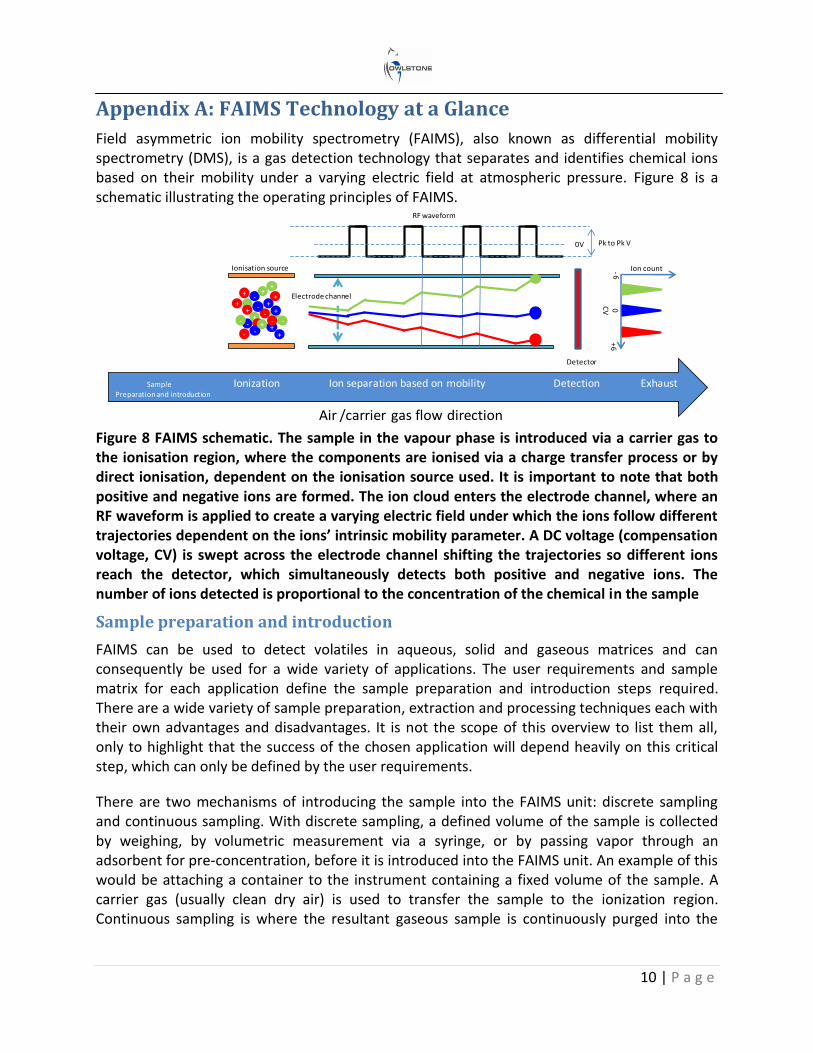
The HHTT calibrations using spiked crude A and B are shown in Figure 6. The offset between the two different oil calibrations can be attributed to the different amount of Sulphur present in each of the oil types. Crude A has less than 0.3% leading to a higher concentration of HHTT than that of crude B which has a Sulphur content of around 3.5% because less of the HHTT is used to scavenge the available Sulphur. As MEA is a by-product of this process it can be used to validate this assumption. The MEA ion count was plotted against the HHTT concentration (Figure 7) and as expected the amount of MEA present is higher in Crude B than that of Crude A.

Figure 6 - HHTT calibrations in crude oil A and B, error bars = 3% sample to sample error

Figure 7 - plot of MEA ion count against HHTT concentration in crude oil A and B, error bars = 1 STDEV where n=6

y = -3E-06x2 + 0.0037xR² = 0.9934

y = -1E-06x2 + 0.0023xR² = 0.9963

0.0

0.2

0.4

0.6

0.8

1.0

1.2

1.4

0 100 200 300 400 500 600 700 800 900

HH

TT Io

n C

ou

nt

/ A

.U.

HHTT Concentration in crude oil/ ppm

Crude Oil A (<0.3% S)

Crude Oil B (~3.5% S)

-0.1

0.0

0.1

0.2

0.3

0.4

0.5

0.6

0 100 200 300 400 500 600 700 800 900

MEA

Io

n C

ou

nt

/ A

.U.

HHTT Concentration in crude oil/ ppm

Crude Oil A (<0.3% S)

Crude Oil B (~3.5% S)

10 | P a g e

Appendix A: FAIMS Technology at a Glance

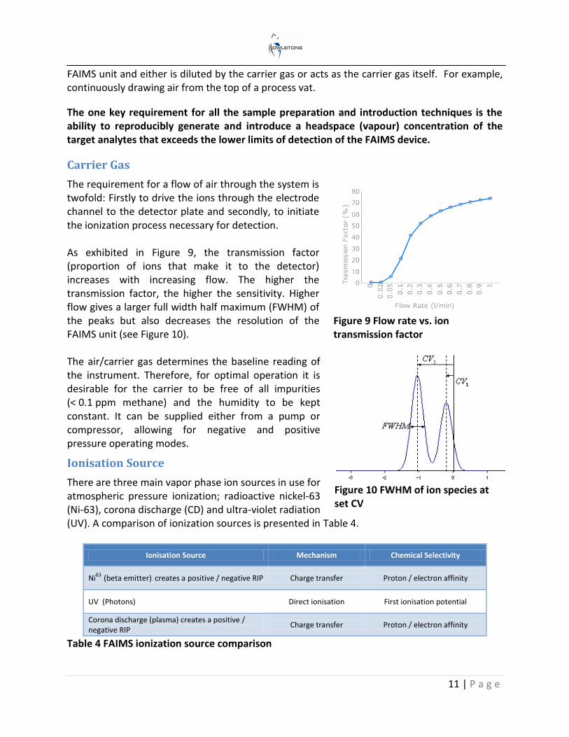
Field asymmetric ion mobility spectrometry (FAIMS), also known as differential mobility spectrometry (DMS), is a gas detection technology that separates and identifies chemical ions based on their mobility under a varying electric field at atmospheric pressure. Figure 8 is a schematic illustrating the operating principles of FAIMS.

Figure 8 FAIMS schematic. The sample in the vapour phase is introduced via a carrier gas to the ionisation region, where the components are ionised via a charge transfer process or by direct ionisation, dependent on the ionisation source used. It is important to note that both positive and negative ions are formed. The ion cloud enters the electrode channel, where an RF waveform is applied to create a varying electric field under which the ions follow different trajectories dependent on the ions’ intrinsic mobility parameter. A DC voltage (compensation voltage, CV) is swept across the electrode channel shifting the trajectories so different ions reach the detector, which simultaneously detects both positive and negative ions. The number of ions detected is proportional to the concentration of the chemical in the sample

Sample preparation and introduction

FAIMS can be used to detect volatiles in aqueous, solid and gaseous matrices and can consequently be used for a wide variety of applications. The user requirements and sample matrix for each application define the sample preparation and introduction steps required. There are a wide variety of sample preparation, extraction and processing techniques each with their own advantages and disadvantages. It is not the scope of this overview to list them all, only to highlight that the success of the chosen application will depend heavily on this critical step, which can only be defined by the user requirements.

There are two mechanisms of introducing the sample into the FAIMS unit: discrete sampling and continuous sampling. With discrete sampling, a defined volume of the sample is collected by weighing, by volumetric measurement via a syringe, or by passing vapor through an adsorbent for pre-concentration, before it is introduced into the FAIMS unit. An example of this would be attaching a container to the instrument containing a fixed volume of the sample. A carrier gas (usually clean dry air) is used to transfer the sample to the ionization region. Continuous sampling is where the resultant gaseous sample is continuously purged into the

-6+

60

Ionisation source

-

-

+

+

+ -

+ +

-

-

-

+

-

-

+

+

+ -

++

-

--

+

CV

Detector

Electrode channel

RF waveform

Air /carrier gas flow direction

Pk to Pk V 0V

Sample Ionization Ion separation based on mobility Detection ExhaustPreparation and introduction

Ion count

11 | P a g e

FAIMS unit and either is diluted by the carrier gas or acts as the carrier gas itself. For example, continuously drawing air from the top of a process vat.

The one key requirement for all the sample preparation and introduction techniques is the ability to reproducibly generate and introduce a headspace (vapour) concentration of the target analytes that exceeds the lower limits of detection of the FAIMS device.

Carrier Gas

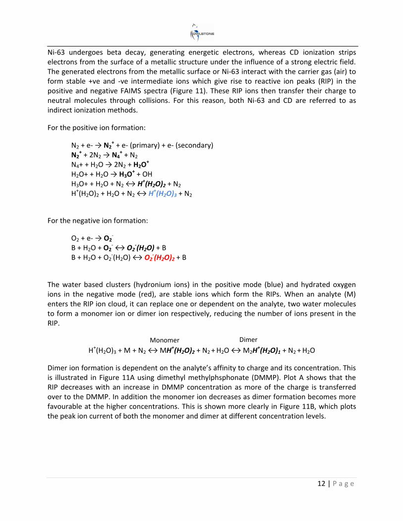
The requirement for a flow of air through the system is twofold: Firstly to drive the ions through the electrode channel to the detector plate and secondly, to initiate the ionization process necessary for detection. As exhibited in Figure 9, the transmission factor (proportion of ions that make it to the detector) increases with increasing flow. The higher the transmission factor, the higher the sensitivity. Higher flow gives a larger full width half maximum (FWHM) of the peaks but also decreases the resolution of the FAIMS unit (see Figure 10). The air/carrier gas determines the baseline reading of the instrument. Therefore, for optimal operation it is desirable for the carrier to be free of all impurities (< 0.1 ppm methane) and the humidity to be kept constant. It can be supplied either from a pump or compressor, allowing for negative and positive pressure operating modes.

Ionisation Source

There are three main vapor phase ion sources in use for atmospheric pressure ionization; radioactive nickel-63 (Ni-63), corona discharge (CD) and ultra-violet radiation (UV). A comparison of ionization sources is presented in Table 4.

Ionisation Source Mechanism Chemical Selectivity

Ni63

(beta emitter) creates a positive / negative RIP Charge transfer Proton / electron affinity

UV (Photons) Direct ionisation First ionisation potential

Corona discharge (plasma) creates a positive / negative RIP

Charge transfer Proton / electron affinity

Table 4 FAIMS ionization source comparison

Figure 9 Flow rate vs. ion transmission factor

Figure 10 FWHM of ion species at set CV

12 | P a g e

Ni-63 undergoes beta decay, generating energetic electrons, whereas CD ionization strips electrons from the surface of a metallic structure under the influence of a strong electric field. The generated electrons from the metallic surface or Ni-63 interact with the carrier gas (air) to form stable +ve and -ve intermediate ions which give rise to reactive ion peaks (RIP) in the positive and negative FAIMS spectra (Figure 11). These RIP ions then transfer their charge to neutral molecules through collisions. For this reason, both Ni-63 and CD are referred to as indirect ionization methods.

For the positive ion formation:

N2 + e- → N2+ + e- (primary) + e- (secondary)

N2+ + 2N2 → N4

+ + N2 N4+ + H2O → 2N2 + H2O+ H2O+ + H2O → H3O+ + OH H3O+ + H2O + N2 ↔ H+(H2O)2 + N2 H+(H2O)2 + H2O + N2 ↔ H+(H2O)3 + N2

For the negative ion formation:

O2 + e- → O2-

B + H2O + O2- ↔ O2

-(H2O) + B B + H2O + O2

-(H2O) ↔ O2-(H2O)2 + B

The water based clusters (hydronium ions) in the positive mode (blue) and hydrated oxygen ions in the negative mode (red), are stable ions which form the RIPs. When an analyte (M) enters the RIP ion cloud, it can replace one or dependent on the analyte, two water molecules to form a monomer ion or dimer ion respectively, reducing the number of ions present in the RIP.

H+(H2O)3 + M + N2 ↔ MH+(H2O)2 + N2 + H2O ↔ M2H

+(H2O)1 + N2 + H2O

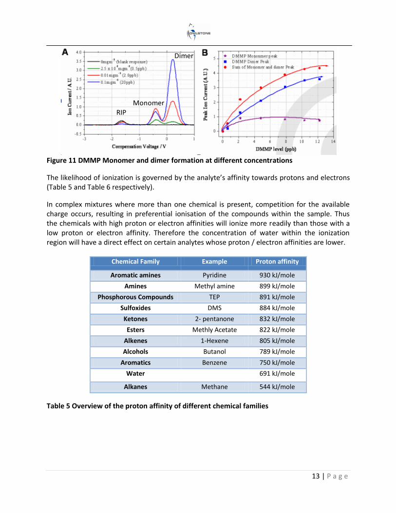
Dimer ion formation is dependent on the analyte’s affinity to charge and its concentration. This is illustrated in Figure 11A using dimethyl methylphsphonate (DMMP). Plot A shows that the RIP decreases with an increase in DMMP concentration as more of the charge is transferred over to the DMMP. In addition the monomer ion decreases as dimer formation becomes more favourable at the higher concentrations. This is shown more clearly in Figure 11B, which plots the peak ion current of both the monomer and dimer at different concentration levels.

Monomer Dimer

13 | P a g e

Figure 11 DMMP Monomer and dimer formation at different concentrations

The likelihood of ionization is governed by the analyte’s affinity towards protons and electrons (Table 5 and Table 6 respectively).

In complex mixtures where more than one chemical is present, competition for the available charge occurs, resulting in preferential ionisation of the compounds within the sample. Thus the chemicals with high proton or electron affinities will ionize more readily than those with a low proton or electron affinity. Therefore the concentration of water within the ionization region will have a direct effect on certain analytes whose proton / electron affinities are lower.

Chemical Family Example Proton affinity

Aromatic amines Pyridine 930 kJ/mole

Amines Methyl amine 899 kJ/mole

Phosphorous Compounds TEP 891 kJ/mole

Sulfoxides DMS 884 kJ/mole

Ketones 2- pentanone 832 kJ/mole

Esters Methly Acetate 822 kJ/mole

Alkenes 1-Hexene 805 kJ/mole

Alcohols Butanol 789 kJ/mole

Aromatics Benzene 750 kJ/mole

Water 691 kJ/mole

Alkanes Methane 544 kJ/mole

Table 5 Overview of the proton affinity of different chemical families

RIP

Monomer

Dimer

14 | P a g e

Chemical Family Electron affinity

Nitrogen Dioxide 3.91eV

Chlorine 3.61eV

Organomercurials

Pesticides

Nitro compounds

Halogenated compounds

Oxygen 0.45eV

Aliphatic alcohols

Ketones

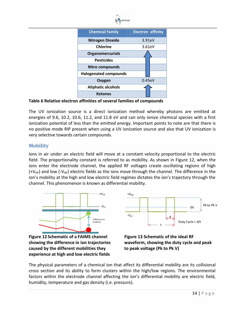
Table 6 Relative electron affinities of several families of compounds

The UV ionization source is a direct ionization method whereby photons are emitted at energies of 9.6, 10.2, 10.6, 11.2, and 11.8 eV and can only ionize chemical species with a first ionization potential of less than the emitted energy. Important points to note are that there is no positive mode RIP present when using a UV ionization source and also that UV ionization is very selective towards certain compounds.

Mobility

Ions in air under an electric field will move at a constant velocity proportional to the electric field. The proportionality constant is referred to as mobility. As shown in Figure 12, when the ions enter the electrode channel, the applied RF voltages create oscillating regions of high (+VHF) and low (-VHF) electric fields as the ions move through the channel. The difference in the ion’s mobility at the high and low electric field regimes dictates the ion’s trajectory through the channel. This phenomenon is known as differential mobility.

Figure 12 Schematic of a FAIMS channel showing the difference in ion trajectories caused by the different mobilities they experience at high and low electric fields

Figure 13 Schematic of the ideal RF waveform, showing the duty cycle and peak to peak voltage (Pk to Pk V)

The physical parameters of a chemical ion that affect its differential mobility are its collisional cross section and its ability to form clusters within the high/low regions. The environmental factors within the electrode channel affecting the ion’s differential mobility are electric field, humidity, temperature and gas density (i.e. pressure).

-VLF

+VHF

Difference in mobility

Pk to Pk V 0V

+VHF

-VLF d

Duty Cycle = d/t t

15 | P a g e

The electric field in the high/low regions is supplied by the applied RF voltage waveform (Figure 13). The duty cycle is the proportion of time spent within each region per cycle. Increasing the peak-to-peak voltage increases/decreases the electric field experienced in the high/low field regions and therefore influences the velocity of the ion accordingly. It is this parameter that has the greatest influence on the differential mobility exhibited by the ion.

It has been shown that humidity has a direct effect on the differential mobility of certain chemicals, by increasing/decreasing the collision cross section of the ion within the respective low/high field regions. The addition and subtraction of water molecules to analyte ions is referred to as clustering and de-clustering. Increased humidity also increases the number of water molecules involved in a cluster (MH+(H2O)2) formed in the ionisation region. When this cluster experiences the high field in between the electrodes the water molecules are forced away from the cluster reducing the size (MH+) (de-clustering). As the low field regime returns so do the water molecules to the cluster, thus increasing the ion’s size (clustering) and giving the ion a larger differential mobility. Gas density and temperature can also affect the ion’s mobility by changing the number of ion-molecule collisions and changing the stability of the clusters, influencing the amount of clustering and de-clustering.

Changes in the electrode channel’s environmental parameters will change the mobility exhibited by the ions. Therefore it is advantageous to keep the gas density, temperature and humidity constant when building detection algorithms based on an ion’s mobility as these factors would need to be corrected for. However, it should be kept in mind that these parameters can also be optimized to gain greater resolution of the target analyte from the background matrix, during the method development process.

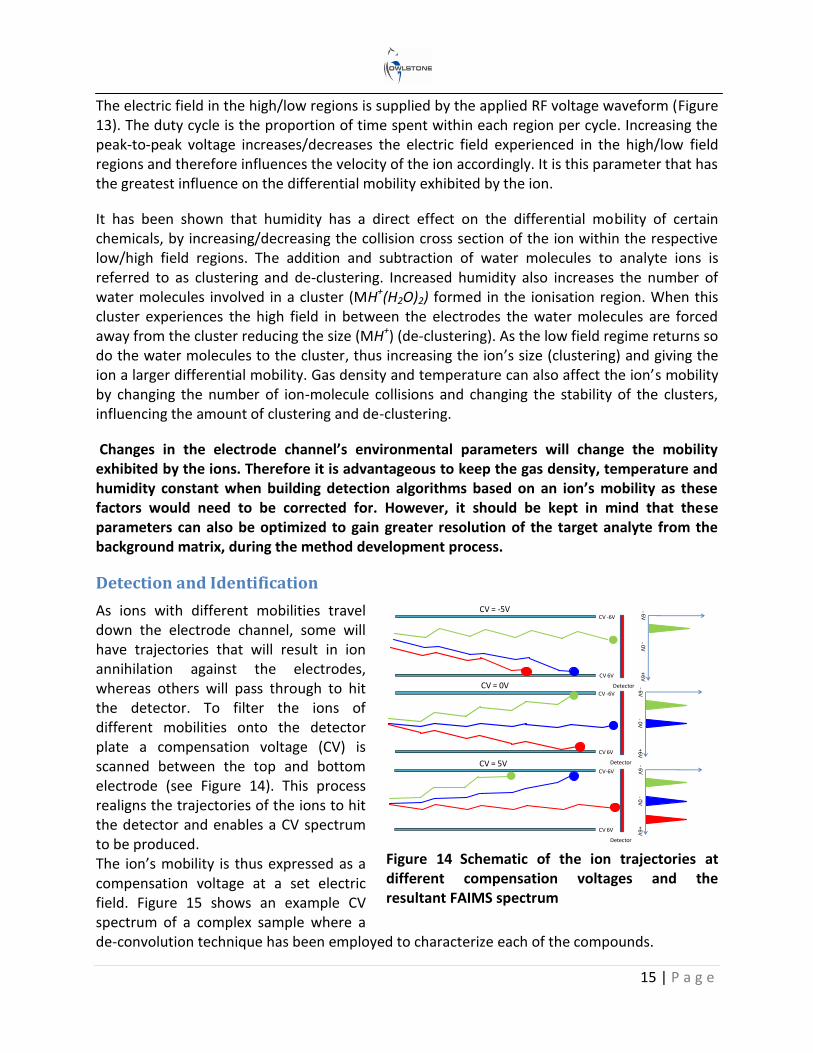
Detection and Identification

As ions with different mobilities travel down the electrode channel, some will have trajectories that will result in ion annihilation against the electrodes, whereas others will pass through to hit the detector. To filter the ions of different mobilities onto the detector plate a compensation voltage (CV) is scanned between the top and bottom electrode (see Figure 14). This process realigns the trajectories of the ions to hit the detector and enables a CV spectrum to be produced. The ion’s mobility is thus expressed as a compensation voltage at a set electric field. Figure 15 shows an example CV spectrum of a complex sample where a de-convolution technique has been employed to characterize each of the compounds.

Figure 14 Schematic of the ion trajectories at different compensation voltages and the resultant FAIMS spectrum

CV -6V

Detector

CV 6V

-6

V+6V

-0V

CV -6V

Detector

CV 6V

-6

V+6

V-

0V

CV-6V

Detector

CV 6V

-6V+6

V-0V

CV = -5V

CV = 0V

CV = 5V

16 | P a g e

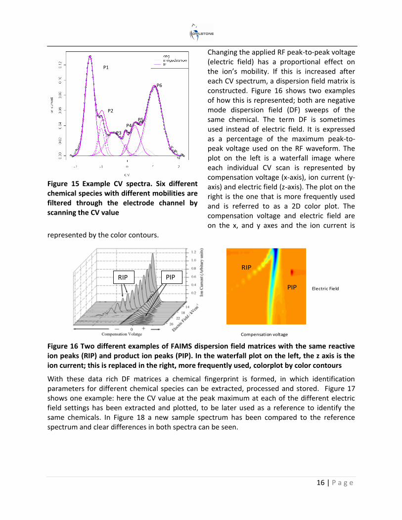
Changing the applied RF peak-to-peak voltage (electric field) has a proportional effect on the ion’s mobility. If this is increased after each CV spectrum, a dispersion field matrix is constructed. Figure 16 shows two examples of how this is represented; both are negative mode dispersion field (DF) sweeps of the same chemical. The term DF is sometimes used instead of electric field. It is expressed as a percentage of the maximum peak-to-peak voltage used on the RF waveform. The plot on the left is a waterfall image where each individual CV scan is represented by compensation voltage (x-axis), ion current (y-axis) and electric field (z-axis). The plot on the right is the one that is more frequently used and is referred to as a 2D color plot. The compensation voltage and electric field are on the x, and y axes and the ion current is

represented by the color contours.

Figure 16 Two different examples of FAIMS dispersion field matrices with the same reactive ion peaks (RIP) and product ion peaks (PIP). In the waterfall plot on the left, the z axis is the ion current; this is replaced in the right, more frequently used, colorplot by color contours

With these data rich DF matrices a chemical fingerprint is formed, in which identification parameters for different chemical species can be extracted, processed and stored. Figure 17 shows one example: here the CV value at the peak maximum at each of the different electric field settings has been extracted and plotted, to be later used as a reference to identify the same chemicals. In Figure 18 a new sample spectrum has been compared to the reference spectrum and clear differences in both spectra can be seen.

PIPRIP

Figure 15 Example CV spectra. Six different chemical species with different mobilities are filtered through the electrode channel by scanning the CV value

Electric Field

Compensation voltage

PIP

RIP

P1

P2

P3

P4 P5

P6

17 | P a g e

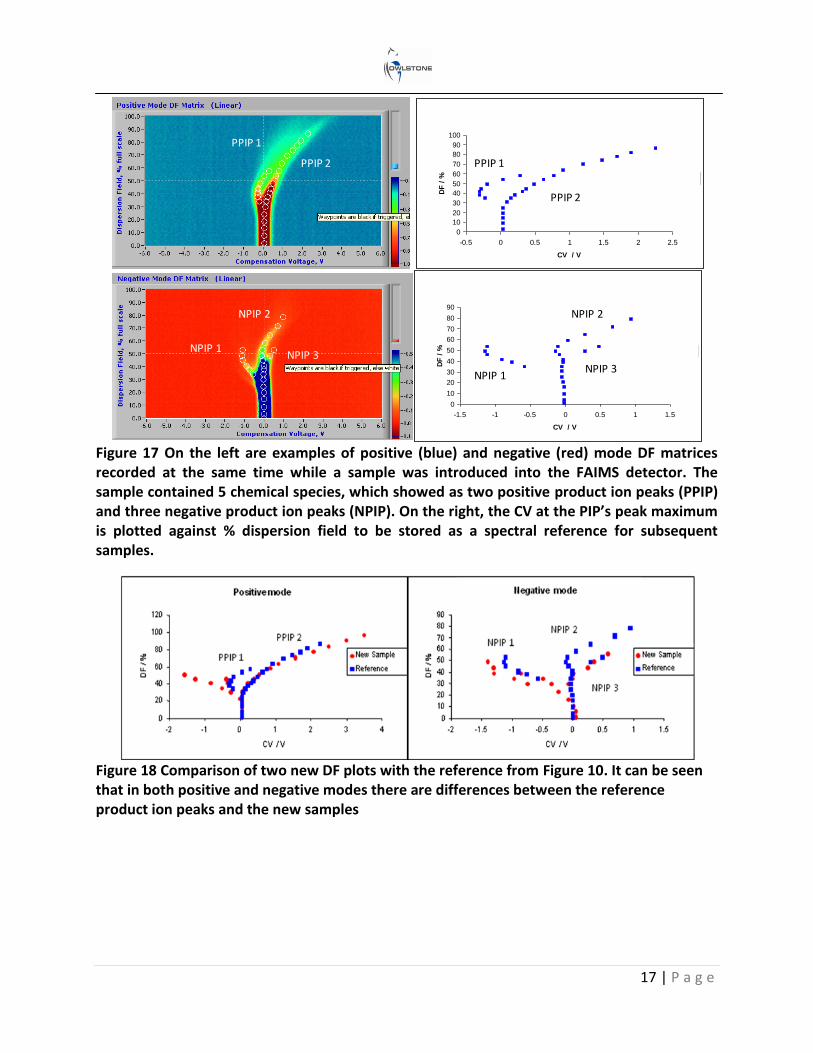
Figure 17 On the left are examples of positive (blue) and negative (red) mode DF matrices recorded at the same time while a sample was introduced into the FAIMS detector. The sample contained 5 chemical species, which showed as two positive product ion peaks (PPIP) and three negative product ion peaks (NPIP). On the right, the CV at the PIP’s peak maximum is plotted against % dispersion field to be stored as a spectral reference for subsequent samples.

Figure 18 Comparison of two new DF plots with the reference from Figure 10. It can be seen that in both positive and negative modes there are differences between the reference product ion peaks and the new samples

0

10

20

30

40

50

60

70

80

90

100

-0.5 0 0.5 1 1.5 2 2.5

CV / V

DF

/ % Pork at 7 Days

0

10

20

30

40

50

60

70

80

90

-1.5 -1 -0.5 0 0.5 1 1.5

CV / V

DF

/ % Pork at 7 Days

PPIP 1

PPIP 2

NPIP 1

NPIP 2

NPIP 3

PPIP 1

PPIP 2

NPIP 1

NPIP 2

NPIP 3

18 | P a g e

Appendix B Generating Calibration Standards with the OVG-4TM Calibration standards can be generated using permeation tubes and Owlstone’s OVG-4 Calibration Gas Generator. The permeation tubes are gravimetrically calibrated to NIST traceable standards. For this study an acetone permeation source was used as a confidence check to ensure the LONESTAR was operating within defined parameters.

The Owlstone OVG-4 is a system for generating NIST traceable chemical and calibration gas standards. It is easy to use, cost-effective and compact and produces a very pure, accurate and repeatable output. The very precise control of concentration levels is achieved using permeation tube technology, eliminating the need for multiple gas cylinders and thus reducing costs, saving space and removing a safety hazard. Complex gas mixtures can be accurately generated through the use of multiple tubes. By swapping out permeation tubes the OVG-4 can be used to generate over 500 calibration standards to test and calibrate almost any gas sensor, instrument or analyzer, including FTIR, NDIR, Raman, IMS, GC, GC/MS. Current customers include – SELEX GALILEO, US Army, US Air Force, US Defense Threat Reduction Agency, Home Office Scientific Development Branch, DSTL, Commissariat à l'Énergie Atomique, EADS, United Technologies, Alphasense, Xtralis, LGC, Genzyme, IEE, Institut de la Corrosion, Rutherford Appleton Laboratory,

University Cambridge, Cranfield among others.

19 | P a g e

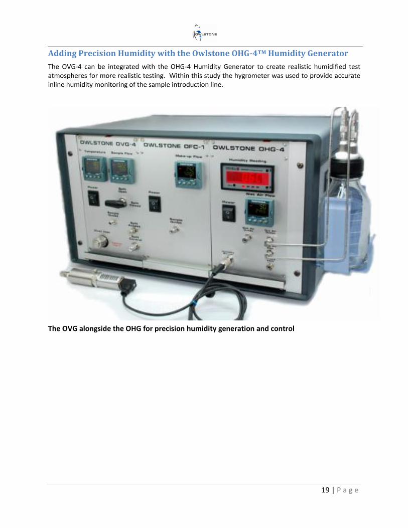
Adding Precision Humidity with the Owlstone OHG-4TM Humidity Generator

The OVG-4 can be integrated with the OHG-4 Humidity Generator to create realistic humidified test atmospheres for more realistic testing. Within this study the hygrometer was used to provide accurate inline humidity monitoring of the sample introduction line.

The OVG alongside the OHG for precision humidity generation and control