Lokale Netzstrukturen - userpages.uni-koblenz.deunikorn/lehre/lone/ws15/01%20Einf%81... ·...

Lokale Netzstrukturen

Einführung

Motivation

WS 13/14 Lokale Netzstrukturen ‐ Einführung 2

Moore’s Law


Exploiting Moore‘s Law wrt. Scale

one mainframe for many desktop PC for one many devices for one

Size Number

4

How to Network many Devices?• Small (and possibly mobile devices) wireless networking

• “Classical” wireless Networking uses base stations– Example: Wireless LAN– Example: Mobile Phones

• Why always relying on an infrastructure?– Less maintenance cost without relying on an infrastructure– Rapid installation of a network if infrastructure is used– Communication would be for free– Not involving a far away base station may even save communication bandwidth

• Try to construct a network without infrastructure, using networking abilities of the participants

• Simplest example: Laptops in a conference room – a single‐hop ad hoc network

• More sophisticated example: multihop ad‐hoc networks


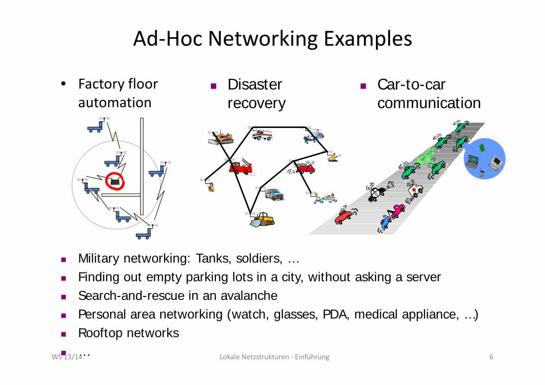
Ad‐Hoc Networking Examples

• Factory floor automation

Disaster recovery

Car-to-car communication

ad ho

c

ad ho

c

Military networking: Tanks, soldiers, … Finding out empty parking lots in a city, without asking a server Search-and-rescue in an avalanche Personal area networking (watch, glasses, PDA, medical appliance, …) Rooftop networks … Lokale Netzstrukturen ‐ EinführungWS 13/14 6

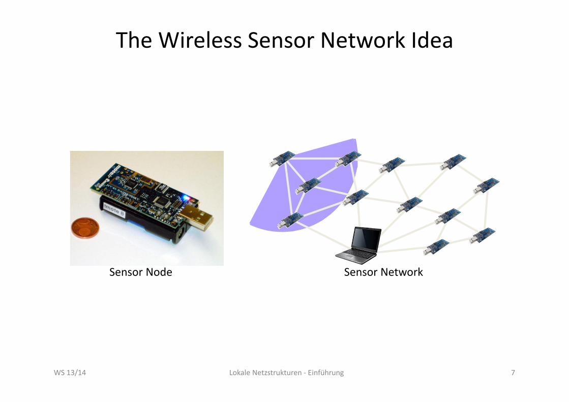
The Wireless Sensor Network Idea

Sensor Node Sensor Network

Lokale Netzstrukturen ‐ EinführungWS 13/14 7

Example: Environmental Monitoring

Example: Great Duck Island, Berkeley, Culler et al.Lokale Netzstrukturen ‐ EinführungWS 13/14 8

Example: Precision Agriculture• Example: LOFAR project

– Fighting Phytophtora using micro‐climate– Temperature and relative humidity


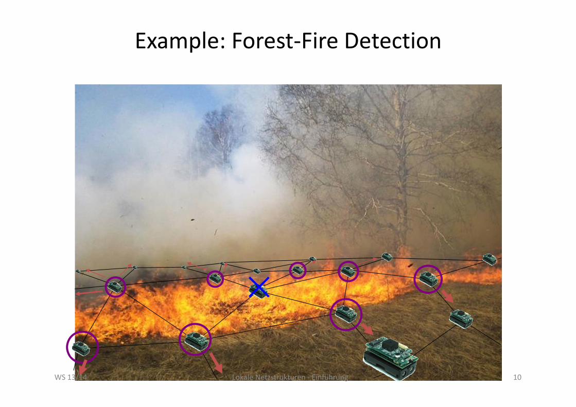
Example: Forest‐Fire Detection


Example: Exploration of Unknown Territory

Example: CotsBots, Berkeley, Pister et al.Lokale Netzstrukturen ‐ EinführungWS 13/14 11

Example: Traffic Telematics

Image source: www.whnet.com/4x4/telematics.htmlLokale Netzstrukturen ‐ EinführungWS 13/14 12

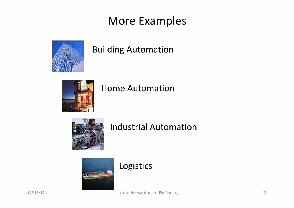
More Examples

Building Automation

Home Automation

Industrial Automation

Logistics


Die Idee der drahtlosen Sensor‐Aktuator‐Netze

Beispiel Gebäudeautomatisierung

Generell: Aktoren in den Beispielanwendungen von Sensornetzen


Idee: Mobile autonome Roboter‐Sensor‐Netze

Beispiel: Überwachung eineskontaminierten Gebietes

Beispiel: Exploration von unerforschtemschwer zugänglichem Gebiet


Idee: Kombinierte mobile Roboter‐ und Sensor‐(Aktuator)‐Netze

Mobile Roboter als drahtloseSupport‐Knoten oder Data‐Mules

Mobile Roboter für Deployment und Maintenance von drahtlosen Sensor‐

(Aktuator)‐Netzen


Herausforderungen

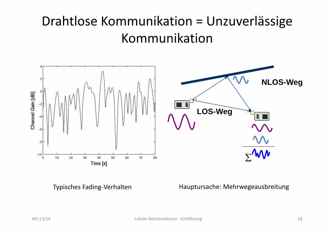
Drahtlose Kommunikation = Unzuverlässige Kommunikation

LOS-Weg

NLOS-Weg

Typisches Fading‐Verhalten Hauptursache: Mehrwegeausbreitung


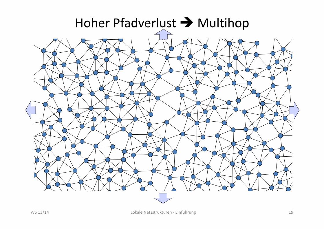
Hoher Pfadverlust Multihop


Sender Receiver

Große Kollisionsdomänen Multihop


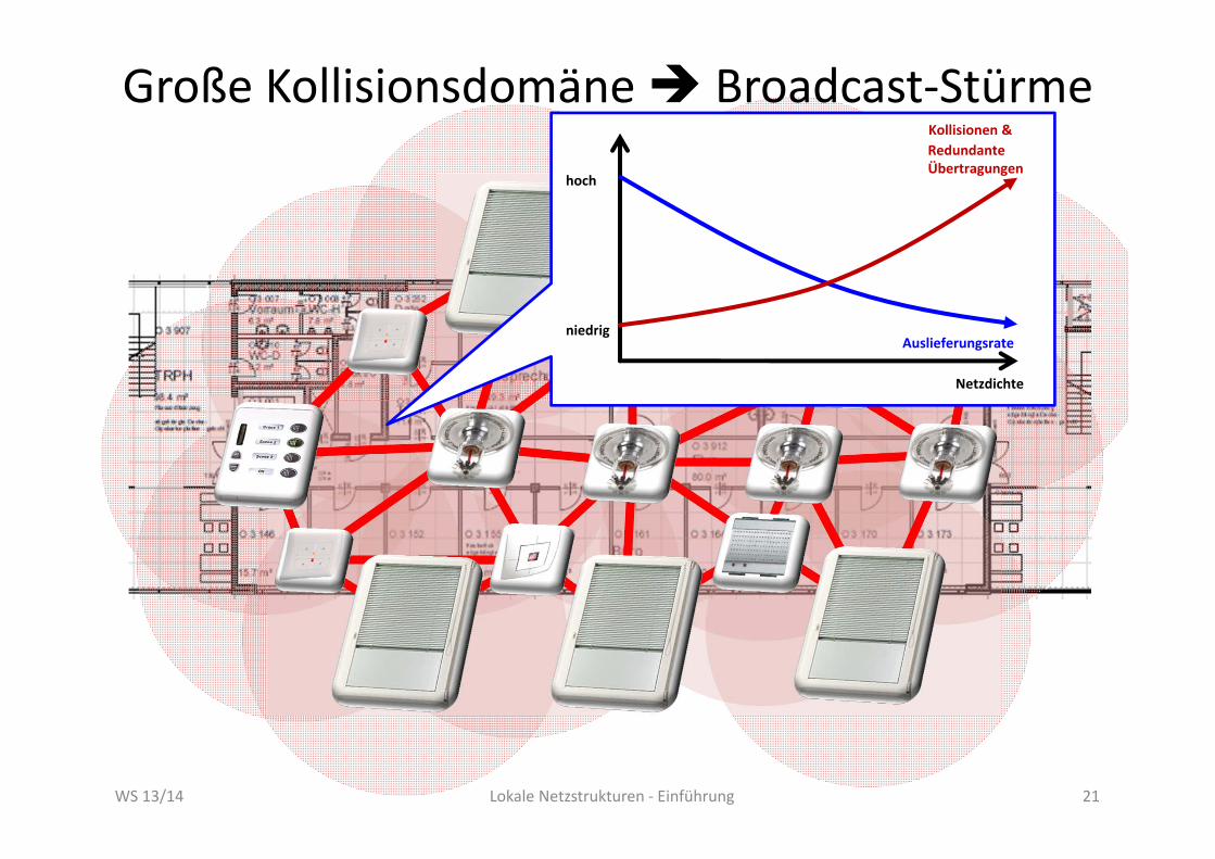
Große Kollisionsdomäne Broadcast‐StürmeRedundanteÜbertragungen

Auslieferungsrate

Kollisionen &

Netzdichte

niedrig

hoch


Limitierender Faktor Batteriekapazität


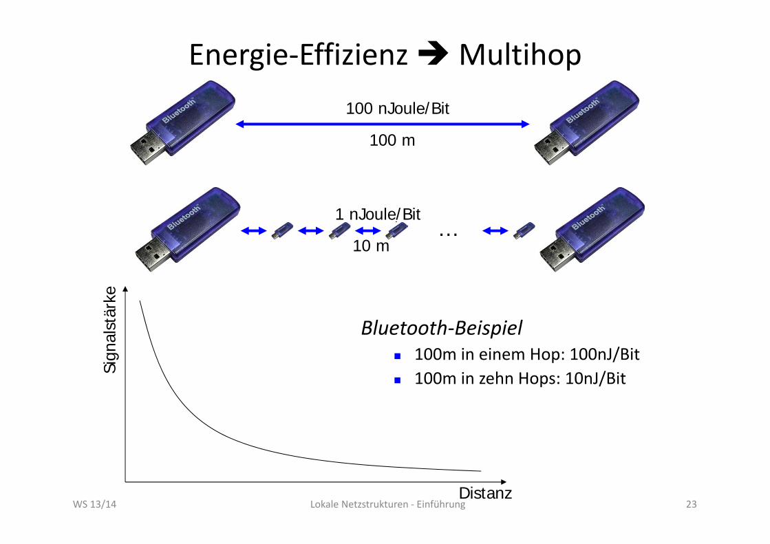
Energie‐Effizienz Multihop

10 m

1 nJoule/Bit…

Bluetooth‐Beispiel 100m in einem Hop: 100nJ/Bit 100m in zehn Hops: 10nJ/Bit

Distanz

Sign

alst

ärke

100 m

100 nJoule/Bit


Energieeffizienz Schalf‐Wach‐Zyklen

Psleep

Pactive

t

P“Traditionelle” MAC-Verfahren:

Psleep

Pactive

t

PEin ideales energieminimales MAC-Verfahren:

Power Consumption

Power Consumption

Power Savings

TX/RX TX/RX TX/RX

TX/RX TX/RX TX/RX


Energieeffizienz In‐Network‐Processing

S3Sink: computemax(d1,d2,d3)

S1

S2

send(d1)

send(d2)

send(d3)

S3 Sink

S1

S2

send(d1)

send(d2)

computem = max(d1,d2,d3)

send(m)

Beispiel: Maximum‐Berechnung

Kommunikationseinsparungen durch DatenaggregationWS 13/14 Lokale Netzstrukturen ‐ Einführung 25

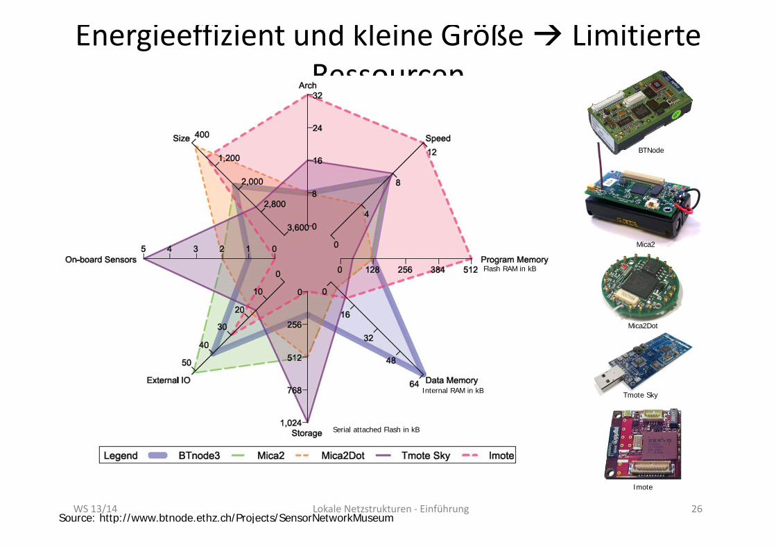
Energieeffizient und kleine Größe Limitierte Ressourcen

BTNode

Mica2

Mica2Dot

Tmote Sky

Imote

Source: http://www.btnode.ethz.ch/Projects/SensorNetworkMuseum

Serial attached Flash in kB

Internal RAM in kB

Flash RAM in kB


Energieeffizient und kleine Größe Limitierte Ressourcen

CC1000 CC1021 CC2420 TR1000 XE1205

Bit Rate[kbps]

76.8 153.6 250 115.2 1.2 - 152.3

Sleep Mode[uA]

0.2 - 1 (osc. core off)

1.8 (core off) 1 0.7 0.2

RX [mA] 9.3 (433MHz) / 11.8 (868MHz)

19.9 19.7 3.8 (115.2kbps)

14

TX Min [mA] 8.6 (-20dBm) 14.5 (-20dBm)

8.5 (-25dBm) 33 (+5dBm)

TX Max [mA] 25.4 (+5dBm)

25.1 (+5dBm)

17.4 (0dBm) 12 (+1.5dBm)

62 (+15dBm)

Source: http://www.btnode.ethz.ch/Projects/SensorNetworkMuseumWS 13/14 Lokale Netzstrukturen ‐ Einführung 27

Mobilität


ModellbildungModellierung einer einzigen Verbindung


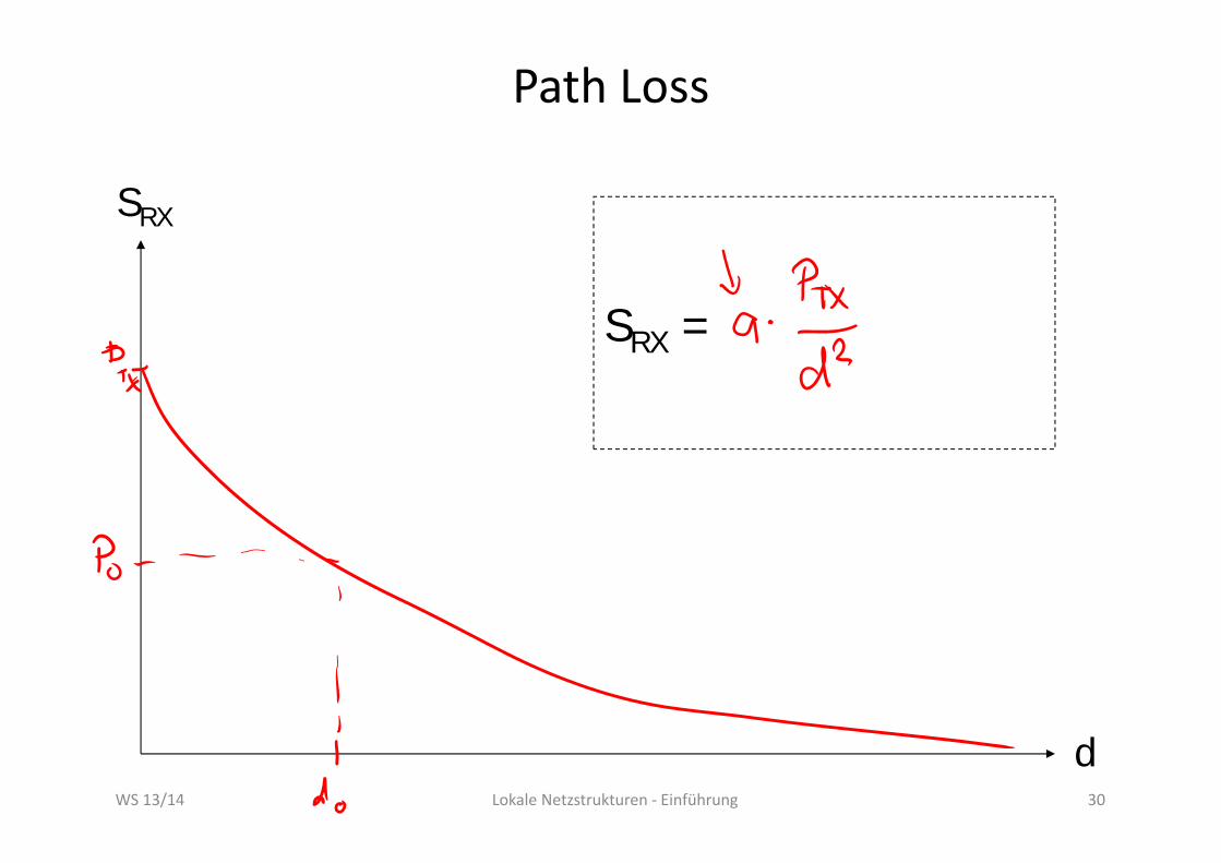
Path Loss

d

SRX

SRX =


Path Loss: A Geometric Explanation


Further Effects

• Reflection & Refraction

• Diffraction

• Scattering

• Doppler Shift


Log‐Distance Path Loss Model


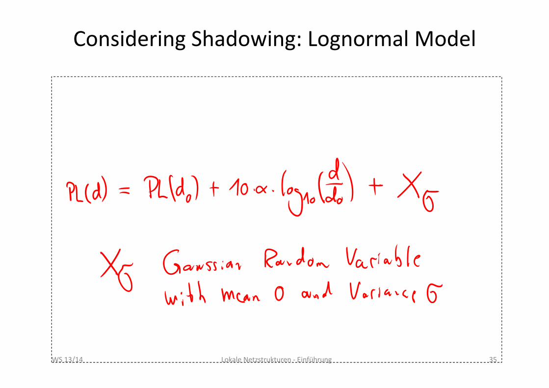
Considering Shadowing: Lognormal Model


36

Modeling the Time Varying Nature• Consider mobile sender receiver pair

• Modeling received signal strength as R.V. X

• Considering probability P[X · x] (the CDF)

• Example: Rayleigh Fading Model– No line of sight– Exponential distributed CDF

• Example: Ricean fading model– Dominant line of sight– Ricean distributed CDF

WS 13/14 Lokale Netzstrukturen ‐ Einführung

ModellbildungEin einfaches Energiemodell


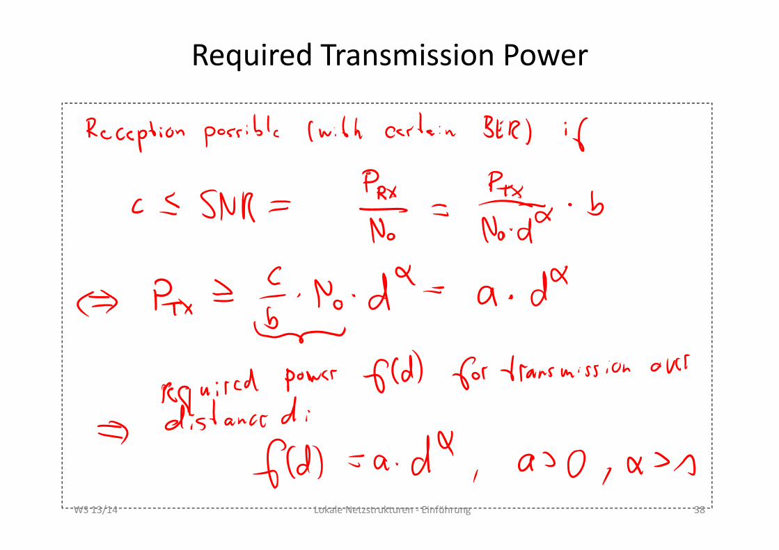
Required Transmission Power


Zero Power with Infinite Relays?

• Direct transmission

• Transmission with n relays

s t

d


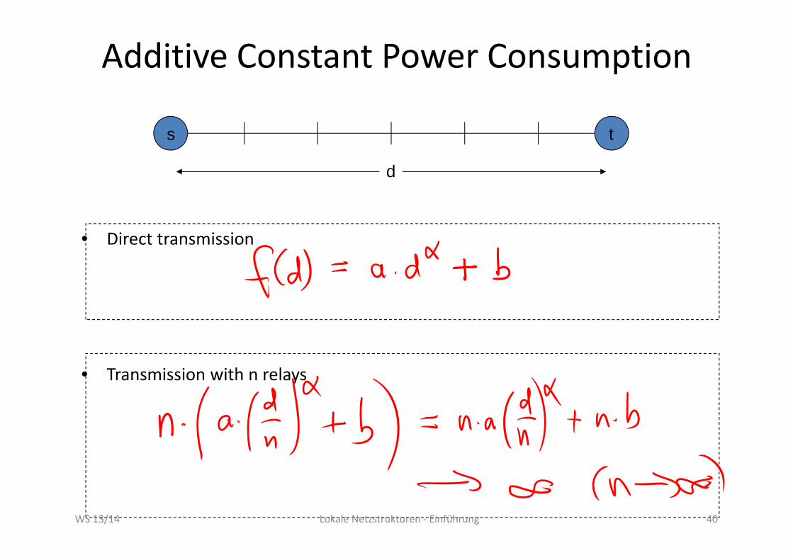
Additive Constant Power Consumption

• Direct transmission

• Transmission with n relays

s t

d


Lokale Netzstrukturen - userpages.uni-koblenz.deunikorn/lehre/lone/ws15/01%20Einf%81... ·...

Documents

Transcript of Lokale Netzstrukturen - userpages.uni-koblenz.deunikorn/lehre/lone/ws15/01%20Einf%81... ·...