Logistics Management

Inventory – Cycle Inventory

Özgür Kabak, Ph.D.

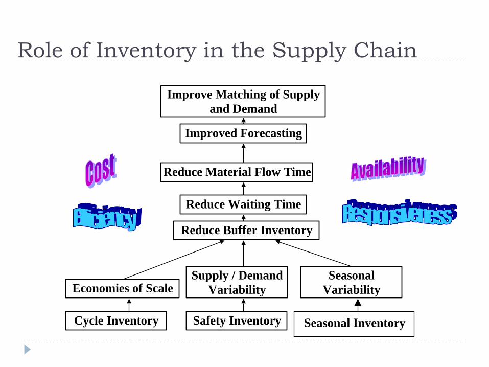
Role of Inventory in the Supply Chain

Improve Matching of Supply

and Demand

Improved Forecasting

Reduce Material Flow Time

Reduce Waiting Time

Reduce Buffer Inventory

Economies of ScaleSupply / Demand

Variability

Seasonal

Variability

Cycle Inventory Safety Inventory

Figure Error! No text of

Seasonal Inventory

What are Inventories?

Finished product held for sale

Goods in warehouses

Work in process

Goods in transit

Staff hired to meet service needs

Any owned or financially controlled raw material,

work in process, and/or finished good or service held

in anticipation of a sale but not yet sold

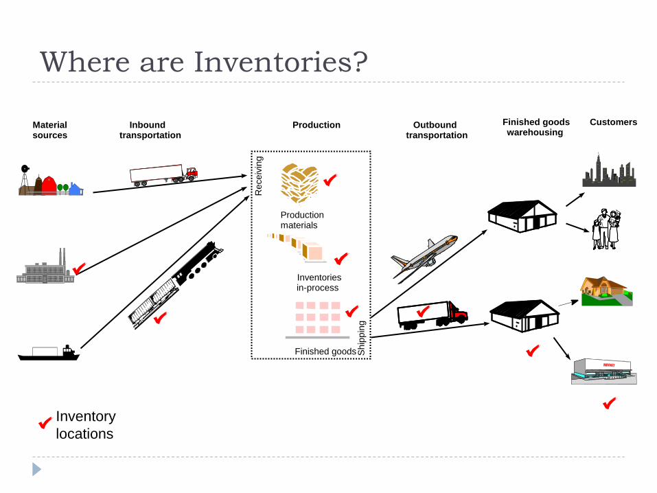
Where are Inventories?

Material sources

Inbound transportation

Production Outbound transportation

Finished goods warehousing

Customers

Inventory

locations

Finished goods Ship

pin

g

Inventories in-process

Receiv

ing

Production materials

Reasons for Inventories Improve customer service

Provides immediacy in product availability

Encourage production, purchase, and transportation economies Allows for long production runs

Takes advantage of price-quantity discounts

Allows for transport economies from larger shipment sizes

Act as a hedge against price changes Allows purchasing to take place under most favorable price terms

Protect against uncertainties in demand and lead times Provides a measure of safety to keep operations running when

demand levels and lead times cannot be known for sure

Act as a hedge against contingencies Buffers against such events as strikes, fires, and disruptions in

supply

Reasons Against Inventories

They consume capital resources that might be put to

better use elsewhere in the firm

They too often mask quality problems that would

more immediately be solved without their presence

They divert management’s attention away from

careful planning and control of the supply and

distribution channels by promoting an insular attitude

about channel management

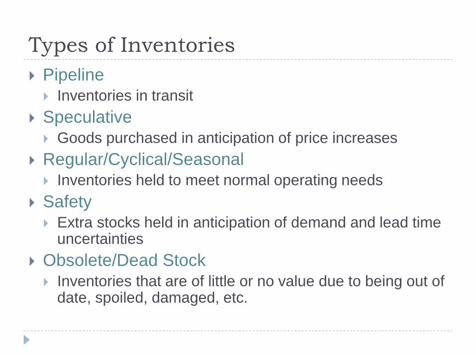
Types of Inventories

Pipeline Inventories in transit

Speculative

Goods purchased in anticipation of price increases

Regular/Cyclical/Seasonal Inventories held to meet normal operating needs

Safety Extra stocks held in anticipation of demand and lead time

uncertainties

Obsolete/Dead Stock

Inventories that are of little or no value due to being out of date, spoiled, damaged, etc.

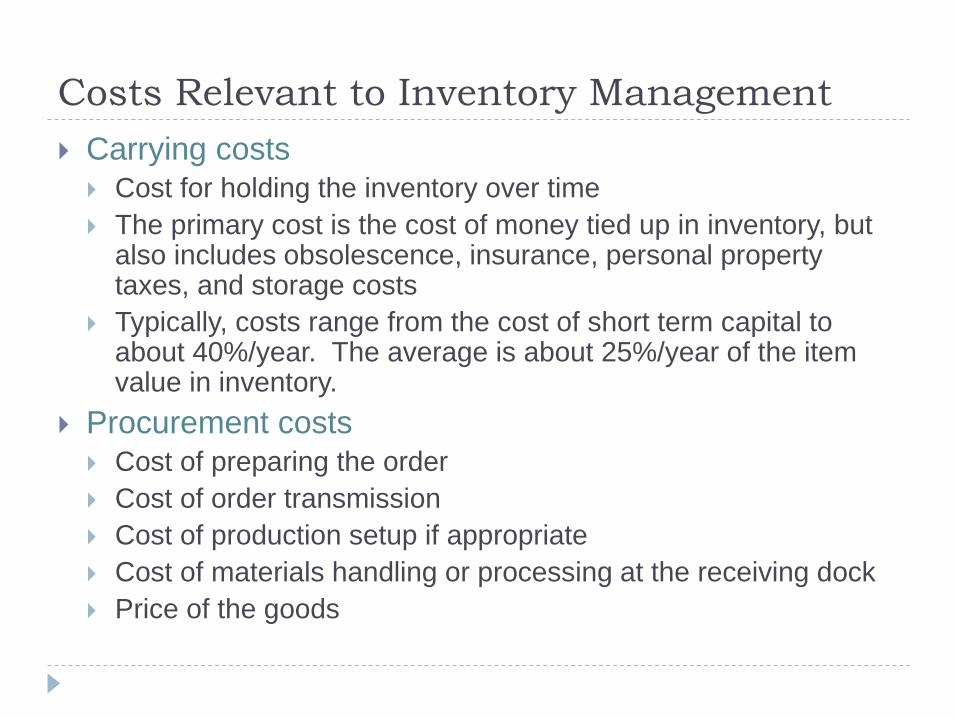
Costs Relevant to Inventory Management

Carrying costs

Cost for holding the inventory over time

The primary cost is the cost of money tied up in inventory, but also includes obsolescence, insurance, personal property taxes, and storage costs

Typically, costs range from the cost of short term capital to about 40%/year. The average is about 25%/year of the item value in inventory.

Procurement costs

Cost of preparing the order

Cost of order transmission

Cost of production setup if appropriate

Cost of materials handling or processing at the receiving dock

Price of the goods

Costs Relevant to Inventory Management

Out-of-stock costs

Lost sales cost

Profit immediately foregone

Future profits foregone through loss of goodwill

Backorder cost

Costs of extra order handling

Additional transportation and handling costs

Possibly additional setup costs

Inventory Management Objectives Good inventory management is a careful balancing act

between stock availability and the cost of holding inventory.

Service objectives Setting stocking levels so that there is only a specified probability

of running out of stock

Cost objectives Balancing conflicting costs to find the most economical

replenishment quantities and timing

Customer Service ,

i.e., Stock Availability Inventory Holding costs

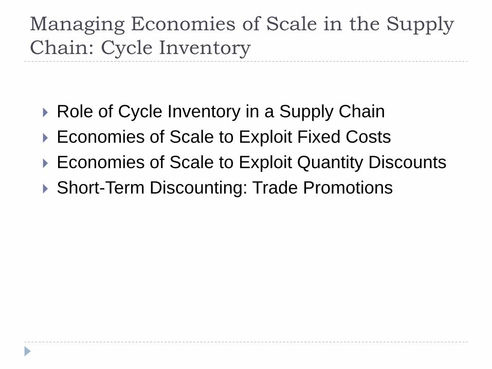
Managing Economies of Scale in the Supply

Chain: Cycle Inventory

Role of Cycle Inventory in a Supply Chain

Economies of Scale to Exploit Fixed Costs

Economies of Scale to Exploit Quantity Discounts

Short-Term Discounting: Trade Promotions

Role of Cycle Inventory

in a Supply Chain

Lot, or batch size: quantity that a supply chain stage either produces or orders at a given time

Cycle inventory: average inventory that builds up in the supply chain because a supply chain stage either produces or purchases in lots that are larger than those demanded by the customer Q = lot or batch size of an order D = demand per unit time

Inventory profile: plot of the inventory level over time

Cycle inventory = Q/2 (depends directly on lot size)

Average flow time = Avg inventory / Avg flow rate Average flow time from cycle inventory = Q/(2D)

Reorder Point Method Under Certainty

for a Single Item

0 Time Lead

time

Lead

time Order

Placed

Order

Placed

Order

Received

Order

Received

Reorder

point, R

Q

Quantity on-hand

plus on-order

Role of Cycle Inventory

in a Supply Chain

Q = 1000 units

D = 100 units/day

Cycle inventory = Q/2 = 1000/2 = 500 = Avg inventory level from cycle inventory

Avg flow time = Q/2D = 1000/(2)(100) = 5 days

Cycle inventory adds 5 days to the time a unit spends in the supply chain

Lower cycle inventory is better because: Average flow time is lower

Working capital requirements are lower

Lower inventory holding costs

Role of Cycle Inventory

in a Supply Chain

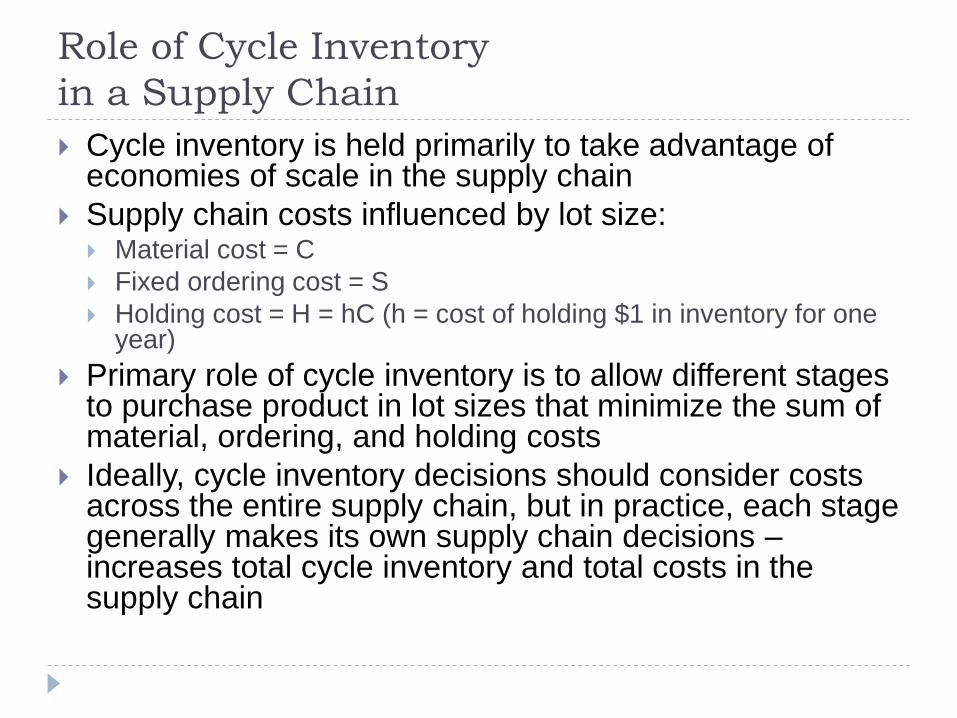
Cycle inventory is held primarily to take advantage of economies of scale in the supply chain

Supply chain costs influenced by lot size: Material cost = C

Fixed ordering cost = S

Holding cost = H = hC (h = cost of holding $1 in inventory for one year)

Primary role of cycle inventory is to allow different stages to purchase product in lot sizes that minimize the sum of material, ordering, and holding costs

Ideally, cycle inventory decisions should consider costs across the entire supply chain, but in practice, each stage generally makes its own supply chain decisions – increases total cycle inventory and total costs in the supply chain

Estimating Cycle Inventory Related Costs in

Practice

Inventory Holding Cost

Obsolescence

Handling costs

Occupancy costs

Theft, security, damage, tax, insurance

Ordering Cost

Buyer time

Transportation costs

Receiving costs

Unique other costs

Economies of Scale

to Exploit Fixed Costs

How do you decide whether to go shopping at a

convenience store or at Sam’s Club?

Lot sizing for a single product (EOQ)

Aggregating multiple products in a single order

Lot sizing with multiple products or customers

Lots are ordered and delivered independently for each

product

Lots are ordered and delivered jointly for all products

Lots are ordered and delivered jointly for a subset of

products

Economies of Scale

to Exploit Fixed Costs

Annual demand = D

Number of orders per year = D/Q

Annual material cost = CD

Annual order cost = (D/Q)S

Annual holding cost = (Q/2)H = (Q/2)hC

Total annual cost = TC = CD + (D/Q)S + (Q/2)hC

Figure 10.2 shows variation in different costs for

different lot sizes at Best Buy

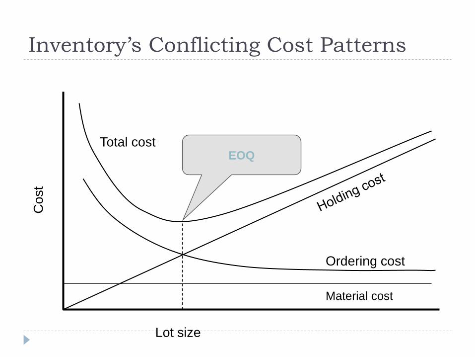
Inventory’s Conflicting Cost Patterns C

ost

Lot size

Material cost

Ordering cost

Total cost EOQ

Fixed Costs: Optimal Lot Size

and Reorder Interval (EOQ)

S

DhCn

H

DSQ

hCH

2*

2*

D: Annual demand

S: Setup or Order Cost

C: Cost per unit

h: Holding cost per year as a fraction of product cost

H: Holding cost per unit per year

Q: Lot Size, Q*: Optimal Lot Size

n*: Optimal order frequency

Material cost is constant and therefore is not considered in this model

Example - EOQ

Demand, D = 12,000 computers per year

Unit cost per lot, C = $500

Holding cost per year as a fraction of unit cost , h = 0.2

Fixed cost, S = $4,000/order

Q* = Sqrt[(2)(12000)(4000)/(0.2)(500)] = 980 computers

Cycle inventory = Q*/2 = 490

Average Flow time = Q*/2D = 980/(2)(12000) = 0.041

year = 0.49 month

n* = Sqrt[(12000)(0.2)(500)/(2)(4000)] = 12.24 orders

Example - EOQ (continued)

Annual ordering and holding cost =

= (12000/980)(4000) + (980/2)(0.2)(500) = $97,980

Suppose lot size is reduced to Q=200, which would reduce flow time:

Annual ordering and holding cost =

= (12000/200)(4000) + (200/2)(0.2)(500) = $250,000

To make it economically feasible to reduce lot size, the fixed cost associated with each lot would have to be reduced

Example – Relationship between desired lot

size and ordering cost

If desired lot size = Q* = 200 units, what would S have

to be?

D = 12000 units

C = $500

h = 0.2

Use EOQ equation and solve for S:

S = [hC(Q*)2]/2D = [(0.2)(500)(200)2]/(2)(12000) =

$166.67

To reduce optimal lot size by a factor of k, the fixed

order cost must be reduced by a factor of k2

Key Points from EOQ Model

In deciding the optimal lot size, the tradeoff is between setup (order) cost and holding cost.

If demand increases by a factor of 4, it is optimal to increase batch size by a factor of 2 and produce (order) twice as often. Cycle inventory (in days of demand) should decrease as demand increases.

If lot size is to be reduced, one has to reduce fixed order cost. To reduce lot size by a factor of 2, order cost has to be reduced by a factor of 4.

Aggregating Multiple Products

in a Single Order

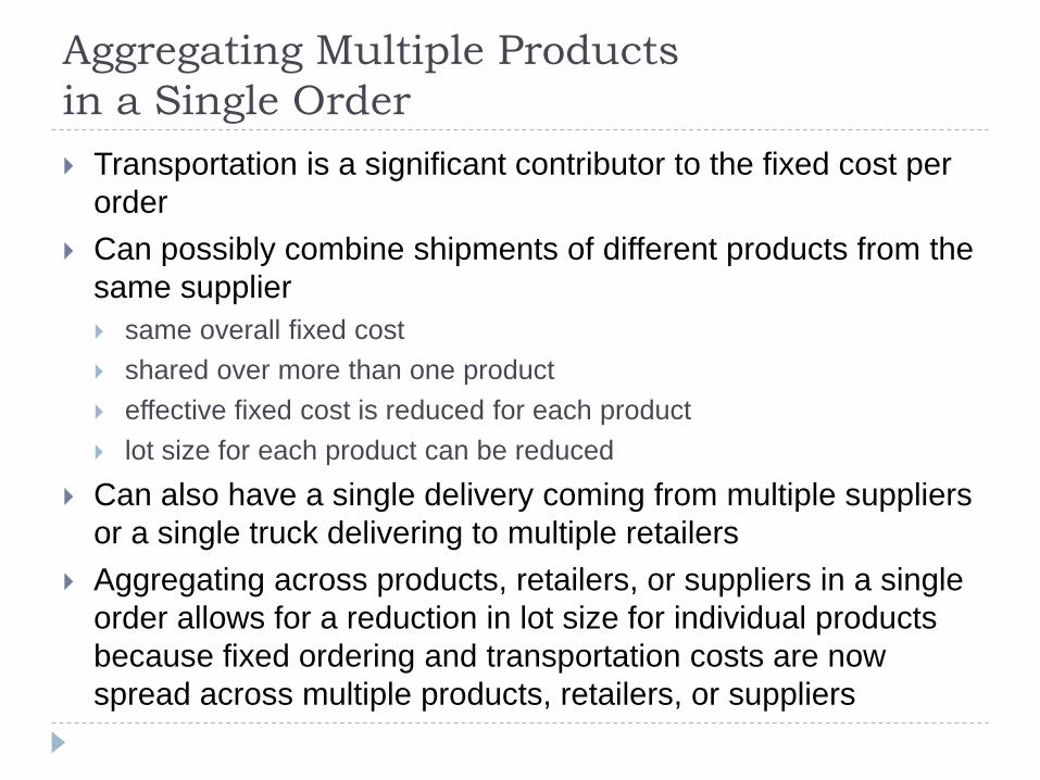
Transportation is a significant contributor to the fixed cost per

order

Can possibly combine shipments of different products from the

same supplier

same overall fixed cost

shared over more than one product

effective fixed cost is reduced for each product

lot size for each product can be reduced

Can also have a single delivery coming from multiple suppliers

or a single truck delivering to multiple retailers

Aggregating across products, retailers, or suppliers in a single

order allows for a reduction in lot size for individual products

because fixed ordering and transportation costs are now

spread across multiple products, retailers, or suppliers

Example: Aggregating Multiple Products in a

Single Order

Suppose there are 4 computer products in the previous

example: Deskpro, Litepro, Medpro, and Heavpro

Assume demand for each is 1000 units per month

If each product is ordered separately:

Q* = 980 units for each product

Total cycle inventory = 4(Q/2) = (4)(980)/2 = 1960 units

Aggregate orders of all four products:

Combined Q* = 1960 units

For each product: Q* = 1960/4 = 490

Cycle inventory for each product is reduced to 490/2 = 245

Total cycle inventory = 1960/2 = 980 units

Average flow time, inventory holding costs will be reduced

Lot Sizing with Multiple

Products or Customers

In practice, the fixed ordering cost is dependent at least in part on the variety associated with an order of multiple models

A portion of the cost is related to transportation (independent of variety)

A portion of the cost is related to loading and receiving (not independent of variety)

Three scenarios:

Lots are ordered and delivered independently for each product

Lots are ordered and delivered jointly for all three models

Lots are ordered and delivered jointly for a selected subset of models

Lot Sizing with Multiple Products

Demand per year

DL = 12,000; DM = 1,200; DH = 120

Common transportation cost, S = $4,000

Product specific order cost

sL = $1,000; sM = $1,000; sH = $1,000

Holding cost, h = 0.2

Unit cost

CL = $500; CM = $500; CH = $500

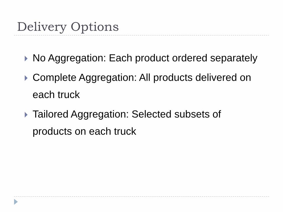
Delivery Options

No Aggregation: Each product ordered separately

Complete Aggregation: All products delivered on

each truck

Tailored Aggregation: Selected subsets of

products on each truck

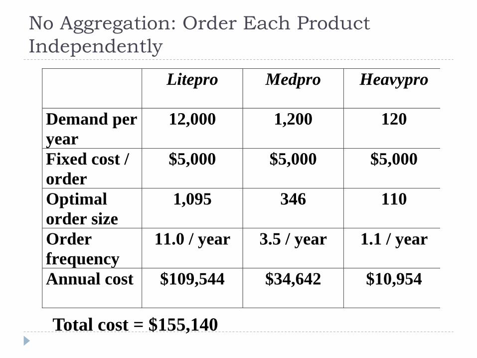
No Aggregation: Order Each Product

Independently

Litepro Medpro Heavypro

Demand per

year

12,000 1,200 120

Fixed cost /

order

$5,000 $5,000 $5,000

Optimal

order size

1,095 346 110

Order

frequency

11.0 / year 3.5 / year 1.1 / year

Annual cost $109,544 $34,642 $10,954

Total cost = $155,140

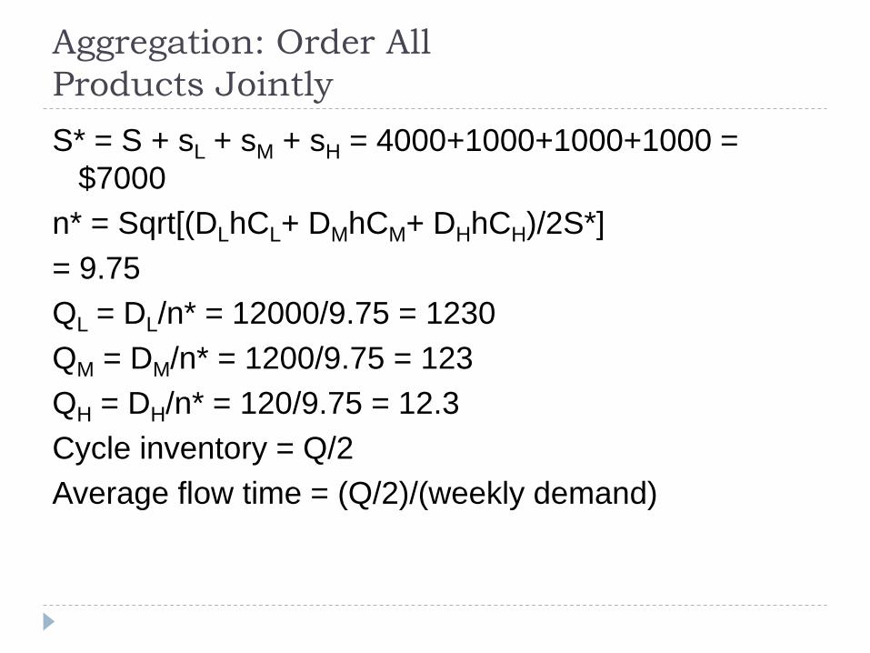
Aggregation: Order All

Products Jointly

S* = S + sL + sM + sH = 4000+1000+1000+1000 =

$7000

n* = Sqrt[(DLhCL+ DMhCM+ DHhCH)/2S*]

= 9.75

QL = DL/n* = 12000/9.75 = 1230

QM = DM/n* = 1200/9.75 = 123

QH = DH/n* = 120/9.75 = 12.3

Cycle inventory = Q/2

Average flow time = (Q/2)/(weekly demand)

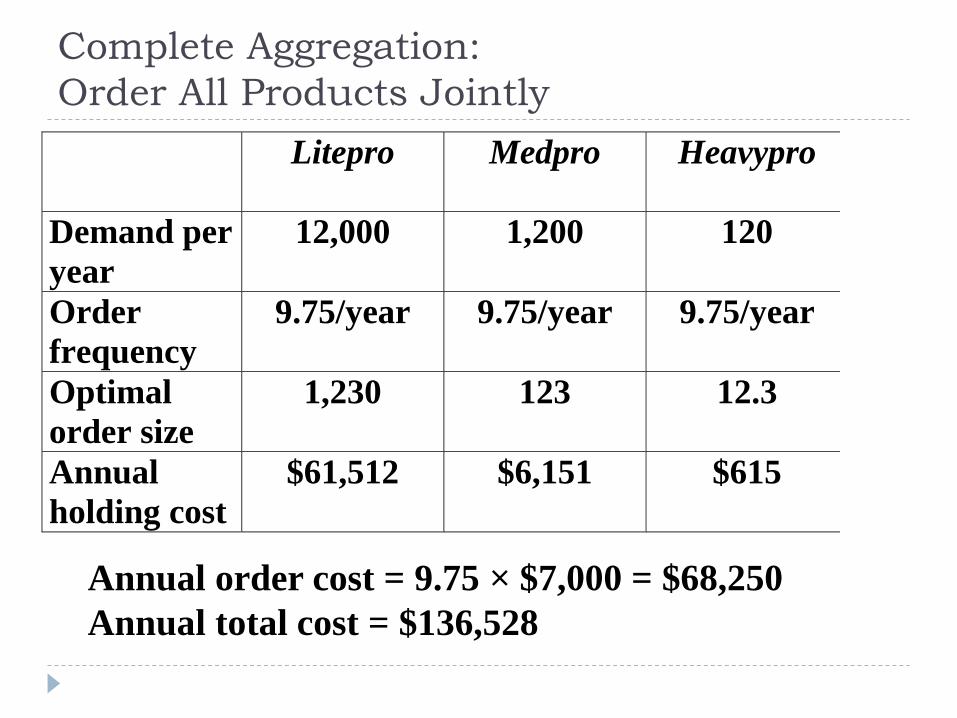
Complete Aggregation:

Order All Products Jointly

Litepro Medpro Heavypro

Demand per

year

12,000 1,200 120

Order

frequency

9.75/year 9.75/year 9.75/year

Optimal

order size

1,230 123 12.3

Annual

holding cost

$61,512 $6,151 $615

Annual order cost = 9.75 × $7,000 = $68,250

Annual total cost = $136,528

Lessons from Aggregation

Aggregation allows firms to lower lot size without

increasing cost

Complete aggregation is effective if product

specific fixed cost is a small fraction of joint fixed

cost

Tailored aggregation is effective if product

specific fixed cost is a large fraction of joint fixed

cost

Economies of Scale to

Exploit Quantity Discounts

All-unit quantity discounts

Marginal unit quantity discounts

Why quantity discounts?

Coordination in the supply chain

Price discrimination to maximize supplier profits

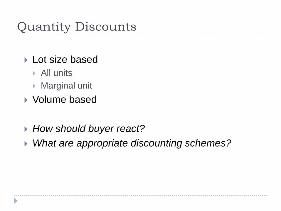
Quantity Discounts

Lot size based

All units

Marginal unit

Volume based

How should buyer react?

What are appropriate discounting schemes?

All-Unit Quantity Discounts

Pricing schedule has specified quantity break points

q0, q1, …, qr, where q0 = 0

If an order is placed that is at least as large as qi but

smaller than qi+1, then each unit has an average unit

cost of Ci

The unit cost generally decreases as the quantity

increases, i.e., C0>C1>…>Cr

The objective for the company (a retailer in our

example) is to decide on a lot size that will minimize

the sum of material, order, and holding costs

All-Unit Quantity Discount Procedure

(different from what is in the textbook)

Step 1: Calculate the EOQ for the lowest price. If it is feasible (i.e., this order quantity is in the range for that price), then stop. This is the optimal lot size. Calculate total cost (TC ) for this lot size.

Step 2: If the EOQ is not feasible, calculate the TC for this price and the smallest quantity for that price.

Step 3: Calculate the EOQ for the next lowest price. If it is feasible, stop and calculate the TC for that quantity and price.

Step 4: Compare the TC for Steps 2 and 3. Choose the quantity corresponding to the lowest TC.

Step 5: If the EOQ in Step 3 is not feasible, repeat Steps 2, 3, and 4 until a feasible EOQ is found.

All-Unit Quantity Discount: Example

Order quantity Unit Price

0-5000 $3.00

5001-10000 $2.96

Over 10000 $2.92

q0 = 0, q1 = 5000, q2 = 10000

C0 = $3.00, C1 = $2.96, C2 = $2.92

D = 120000 units/year, S = $100/lot, h = 0.2

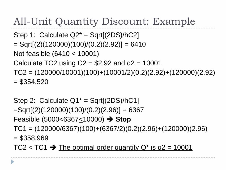
All-Unit Quantity Discount: Example

Step 1: Calculate Q2* = Sqrt[(2DS)/hC2]

= Sqrt[(2)(120000)(100)/(0.2)(2.92)] = 6410

Not feasible (6410 < 10001)

Calculate TC2 using C2 = $2.92 and q2 = 10001

TC2 = (120000/10001)(100)+(10001/2)(0.2)(2.92)+(120000)(2.92)

= $354,520

Step 2: Calculate Q1* = Sqrt[(2DS)/hC1]

=Sqrt[(2)(120000)(100)/(0.2)(2.96)] = 6367

Feasible (5000<6367<10000) Stop

TC1 = (120000/6367)(100)+(6367/2)(0.2)(2.96)+(120000)(2.96)

= $358,969

TC2 < TC1 The optimal order quantity Q* is q2 = 10001

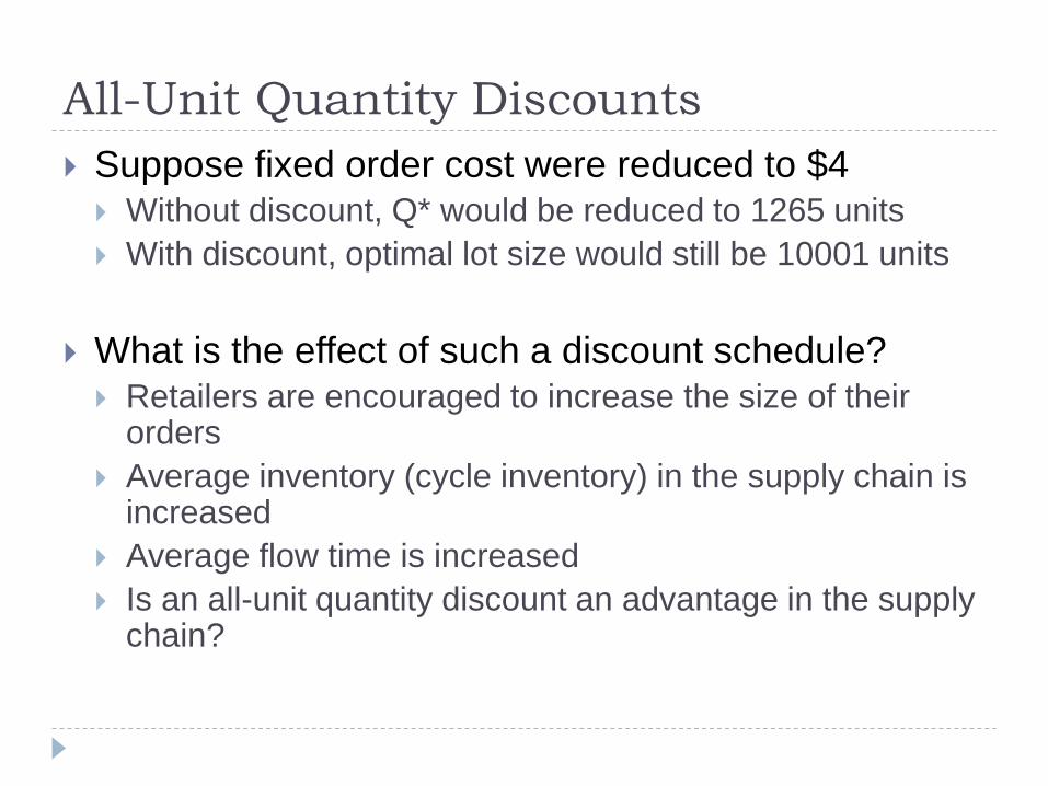
All-Unit Quantity Discounts

Suppose fixed order cost were reduced to $4 Without discount, Q* would be reduced to 1265 units

With discount, optimal lot size would still be 10001 units

What is the effect of such a discount schedule? Retailers are encouraged to increase the size of their

orders

Average inventory (cycle inventory) in the supply chain is increased

Average flow time is increased

Is an all-unit quantity discount an advantage in the supply chain?

Why Quantity Discounts?

Coordination in the supply chain

Commodity products

Products with demand curve

2-part tariffs

Volume discounts

Coordination for

Commodity Products

D = 120,000 bottles/year

SR = $100, hR = 0.2, CR = $3

SS = $250, hS = 0.2, CS = $2

Retailer’s optimal lot size = 6,324 bottles

Retailer cost = $3,795; Supplier cost = $6,009

Supply chain cost = $9,804

Supplier Retailer Coordinate

D 120000 120000 120000

S 250 100 350

h 0,2 0,2 0,2

c 2 3 5 Q* 12247 6324 9165

Coordination for

Commodity Products

What can the supplier do to decrease supply chain

costs?

Coordinated lot size: 9,165; Retailer cost = $4,059;

Supplier cost = $5,106; Supply chain cost = $9,165

Effective pricing schemes

All-unit quantity discount

$3 for lots below 9,165

$2.9978 for lots of 9,165 or more

Pass some fixed cost to retailer (enough that he raises

order size from 6,324 to 9,165)

Quantity Discounts When

Firm Has Market Power

No inventory related costs

Demand curve

360,000 - 60,000p

What are the optimal prices and profits in the following

situations?

Production cost: $2

Stages: Manucturer and Retailer

The two stages coordinate the pricing decision

Price = $4, Profit = $240,000, Demand = 120,000

The two stages make the pricing decision independently

Price = $5, Profit = $180,000, Demand = 60,000

Two-Part Tariffs and

Volume Discounts

Design a two-part tariff that achieves the coordinated

solution

Design a volume discount scheme that achieves the

coordinated solution

Impact of inventory costs

Pass on some fixed costs with above pricing

Two part Trafiffs: fixed $180,000 + $2 per bottle

Valume based discount:

if less then 120,000 : $4

If equal or greater than 120,000: $3.5

Lessons from Discounting Schemes

Lot size based discounts increase lot size and cycle

inventory in the supply chain

Lot size based discounts are justified to achieve

coordination for commodity products

Volume based discounts with some fixed cost

passed on to retailer are more effective in general

Volume based discounts are better over rolling horizon

Short-Term Discounting:

Trade Promotions

Trade promotions are price discounts for a limited period of time (also may require specific actions from retailers, such as displays, advertising, etc.)

Key goals for promotions from a manufacturer’s perspective: Induce retailers to use price discounts, displays, advertising to

increase sales

Shift inventory from the manufacturer to the retailer and customer

Defend a brand against competition

Goals are not always achieved by a trade promotion

What is the impact on the behavior of the retailer and on the performance of the supply chain?

Retailer has two primary options in response to a promotion: Pass through some or all of the promotion to customers to spur sales

Purchase in greater quantity during promotion period to take advantage of temporary price reduction, but pass through very little of savings to customers

Short Term Discounting

Q*: Normal order quantity

C: Normal unit cost

d: Short term discount

D: Annual demand

h: Cost of holding $1 per year

Qd: Short term order quantity

Forward buy = Qd - Q*

dC

C

hdC

dD QQ

d

-+

)-(=

*

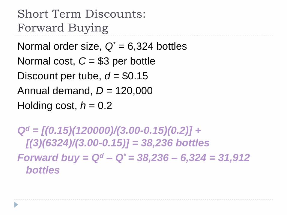
Short Term Discounts:

Forward Buying

Normal order size, Q* = 6,324 bottles

Normal cost, C = $3 per bottle

Discount per tube, d = $0.15

Annual demand, D = 120,000

Holding cost, h = 0.2

Qd = [(0.15)(120000)/(3.00-0.15)(0.2)] +

[(3)(6324)/(3.00-0.15)] = 38,236 bottles

Forward buy = Qd – Q* = 38,236 – 6,324 = 31,912

bottles

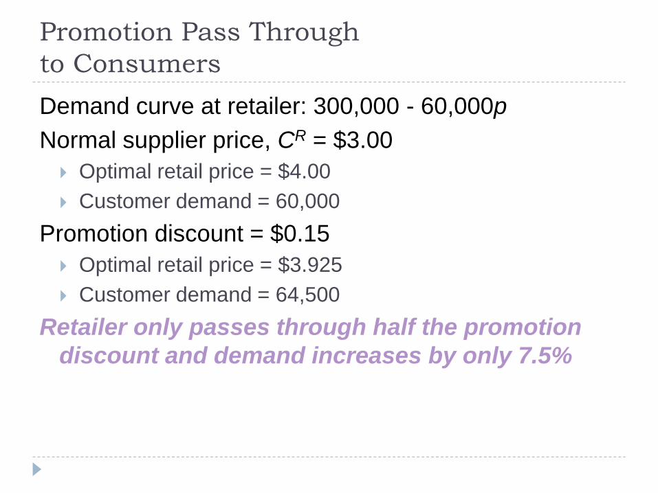
Promotion Pass Through

to Consumers

Demand curve at retailer: 300,000 - 60,000p

Normal supplier price, CR = $3.00

Optimal retail price = $4.00

Customer demand = 60,000

Promotion discount = $0.15

Optimal retail price = $3.925

Customer demand = 64,500

Retailer only passes through half the promotion

discount and demand increases by only 7.5%

Summary of Learning Objectives

How are the appropriate costs balanced to choose the optimal amount of cycle inventory in the supply chain?

What are the effects of quantity discounts on lot size and cycle inventory?

What are appropriate discounting schemes for the supply chain, taking into account cycle inventory?

What are the effects of trade promotions on lot size and cycle inventory?

What are managerial levers that can reduce lot size and cycle inventory without increasing costs?

Next Class

Assignment 1 is uploaded! Due date is next week!

Safety Inventory