Logical Methods in Computer Science Vol. 4 (4:2) …Logical Methods in Computer Science Vol. 4 (4:2)...
68
Logical Methods in Computer Science Vol. 4 (4:2) 2008, pp. 1–68 www.lmcs-online.org Submitted Sep. 23, 2007 Published Oct. 20, 2008 LOGICAL REASONING FOR HIGHER-ORDER FUNCTIONS WITH LOCAL STATE NOBUKO YOSHIDA a , KOHEI HONDA b , AND MARTIN BERGER c a,c Department of Computing, Imperial College London, 180 Queen’s Gate, London, 2AZ SW7 e-mail address: {yoshida,M.Berger}@doc.ic.ac.uk b Department of Computer Science, Queen Mary, University of London, Mile End Road, London, 1E 4NS e-mail address: [email protected] ABSTRACT. We introduce an extension of Hoare logic for call-by-value higher-order functions with ML-like local reference generation. Local references may be generated dynamically and exported outside their scope, may store higher-order functions and may be used to construct complex muta- ble data structures. This primitive is captured logically using a predicate asserting reachability of a reference name from a possibly higher-order datum and quantifiers over hidden references. We ex- plore the logic’s descriptive and reasoning power with non-trivial programming examples combining higher-order procedures and dynamically generated local state. Axioms for reachability and local invariant play a central role for reasoning about the examples. CONTENTS 1. Introduction 3 2. Assertions for Local State 6 2.1. A Programming Language 6 2.2. A Logical Language 7 2.3. Assertions for Local State 10 3. Models and Semantics 12 3.1. Models 12 3.2. Semantics of Equality 14 3.3. Semantics of Necessity and Possibility Operators 16 3.4. Semantics of Evaluation Formulae 16 3.5. Semantics of Universal and Existential Quantification 17 3.6. Semantics of Hiding 18 3.7. Semantics of Content Quantification 18 3.8. Semantics of Reachability 19 3.9. Thin and Stateless Formulae 20 4. Proof Rules and Soundness 23 4.1. Hoare Triples 23 1998 ACM Subject Classification: D.3.1, D.3.3, D.3.2, F.3.1, F.3.2, F.4.1. Key words and phrases: Languages, Theory, Verification. LOGICAL METHODS IN COMPUTER SCIENCE DOI:10.2168/LMCS-4 (4:2) 2008 c N. Yoshida, K. Honda, and M. Berger CC Creative Commons
Transcript of Logical Methods in Computer Science Vol. 4 (4:2) …Logical Methods in Computer Science Vol. 4 (4:2)...

Logical Methods in Computer ScienceVol. 4 (4:2) 2008, pp. 1–68www.lmcs-online.org
Submitted Sep. 23, 2007Published Oct. 20, 2008
LOGICAL REASONING FOR HIGHER-ORDER FUNCTIONS WITH LOCAL ST ATE
NOBUKO YOSHIDAa, KOHEI HONDAb, AND MARTIN BERGERc
a,c Department of Computing, Imperial College London, 180 Queen’s Gate, London, 2AZ SW7e-mail address: yoshida,[email protected]
b Department of Computer Science, Queen Mary, University of London, Mile End Road, London, 1E 4NSe-mail address: [email protected]
ABSTRACT. We introduce an extension of Hoare logic for call-by-valuehigher-order functions withML-like local reference generation. Local references may be generated dynamically and exportedoutside their scope, may store higher-order functions and may be used to construct complex muta-ble data structures. This primitive is captured logically using a predicate asserting reachability of areference name from a possibly higher-order datum and quantifiers over hidden references. We ex-plore the logic’s descriptive and reasoning power with non-trivial programming examples combininghigher-order procedures and dynamically generated local state. Axioms for reachability and localinvariant play a central role for reasoning about the examples.
CONTENTS
1. Introduction 32. Assertions for Local State 62.1. A Programming Language 62.2. A Logical Language 72.3. Assertions for Local State 103. Models and Semantics 123.1. Models 123.2. Semantics of Equality 143.3. Semantics of Necessity and Possibility Operators 163.4. Semantics of Evaluation Formulae 163.5. Semantics of Universal and Existential Quantification 173.6. Semantics of Hiding 183.7. Semantics of Content Quantification 183.8. Semantics of Reachability 193.9. Thin and Stateless Formulae 204. Proof Rules and Soundness 234.1. Hoare Triples 23
1998 ACM Subject Classification:D.3.1, D.3.3, D.3.2, F.3.1, F.3.2, F.4.1.Key words and phrases:Languages, Theory, Verification.
LOGICAL METHODSl IN COMPUTER SCIENCE DOI:10.2168/LMCS-4 (4:2) 2008
c© N. Yoshida, K. Honda, and M. BergerCC© Creative Commons

2 N. YOSHIDA, K. HONDA, AND M. BERGER
4.2. Proof Rules 234.3. Located Judgements 254.4. Invariance Rules for Reachability 264.5. Soundness 275. Axioms and Local Invariants 285.1. Axioms for Equality 285.2. Axioms for Necessity Operators 295.3. Axioms for Hiding 305.4. Axioms for Reachability 315.5. Local Invariants 336. Reasoning Examples 356.1. New Reference Declaration 356.2. Shared Stored Function 366.3. Memoised Factorial 376.4. Information Hiding (2): Stored Circular Procedures 386.5. Mutually Recursive Stored Functions 396.6. Higher-Order Invariant 406.7. Nested Local Invariant from [34,27] 416.8. Information Hiding (5): Object 427. Extension, Related Work and Future Topics 437.1. Three Completeness Results 437.2. Local Variables in Hoare Logic 437.3. Related Work and Future Topics 43References 46Appendix A. Typing Rules 49Appendix B. Proof Rules 51B.1. Proofs of Soundness 52B.2. Soundness of the Invariant Rule 55B.3. Soundness of [LetOpen] and [Subs] 56Appendix C. Soundness of the Axioms 56C.1. Proofs of Lemma 5.1 57C.2. Proof of Proposition 5.3 57C.3. Axioms for Content Quantification 59C.4. Proof of Proposition 5.8 59C.5. Proof of Theorem 5.10 61C.6. Proof of Proposition 5.14 62C.7. Proof of Propositions 5.15 63C.8. Proof of Proposition 5.16 65C.9. Proof of Proposition 5.17 65Appendix D. Derivations for Examples in Section 6 65D.1. Derivation formutualParity 66D.2. Derivation for Meyer-Sieber 67D.3. Derivation for Object 67

LOGICAL REASONING FOR HIGHER-ORDER FUNCTIONS WITH LOCAL STATE 3
1. INTRODUCTION
Reference Generation in Higher-Order Programming. This paper proposes an extension ofHoare Logic [17] for call-by-value higher-order functionswith ML-like new reference generation[1, 2], and demonstrates its use through non-trivial reasoning examples. New reference generation,embodied for example in ML’sref-construct, is a highly expressive programming primitive.Thefirst key functionality of this construct is to introduce local state into the dynamics of programs bygenerating a fresh reference inaccessible from the outside. Consider the following program:
Incdef= let x = ref(0) in λ().(x :=!x+1; !x) (1.1)
where “ref(M)” returns a fresh reference whose content is the value whichM evaluates to; “!x”denotes dereferencing the imperative variablex; and “;” is sequential composition. In (1.1), a ref-erence with content 0 is newly created, but never exported tothe outside. When the anonymousfunction in Inc is invoked, it increments the content of the local variablex, and returns the newcontent. The procedure returns a different result at each call, whose source is hidden from externalobservers. This is different fromλ().(x :=!x+1; !x) wherex is globally accessible.
Secondly, local references may be exported outside of theiroriginal scope and be shared, con-tributing to the expressivity of significant imperative idioms. Let us show how stored proceduresinteract with new reference generation and sharing of references. We consider the following pro-gram from [49, § 6]:
incShareddef= a:=Inc;b:=!a;z1 :=(!a)();z2 :=(!b)();(!z1+!z2) (1.2)
The initial content of the hiddenx is 0. Following the standard semantics of ML [38], the assignmentb :=!a copies the code (or a pointer to the code) froma to b while sharing the storex. Hence thecontent ofx is incremented every time the functions stored ina andb, sharing the same storex,are called, returning 3 at the end of the programincShared. To understand the behaviour ofincShared precisely and give it an appropriate specification, we must capture the sharing ofxbetween the procedures assigned toa and b. From the viewpoint of visibility, the scope ofx isoriginally restricted to the function stored ina but gets extruded to and shared by the one stored inb. If we replaceb :=!a by b := Inc as follows, two separate instances ofInc (hence with separatehidden stores) are assigned toa andb, and the final result is not 3 but 2.
incUnShareddef= a:=Inc;b:=Inc;z1 :=(!a)();z2 :=(!b)();(!z1+!z2) (1.3)
Controlling the sharing of local references is essential for writing concise algorithms that manipulatefunctions with shared store, or mutable data structures such as trees and graphs, but complicatesformal reasoning, even for relatively small programs [18, 34, 36].
Thirdly, through information hiding, local references canbe used for efficient implementationsof highly regular observable behaviour, for example, purely functional behaviour. The followingprogram, taken from [49, § 1], calledmemFact, is a simple memoised factorial.
memFactdef= let a = ref(0), b = ref(1) in
λx.if x =!a then !b else (a := x; b := fact(x) ; !b) (1.4)
Herefact is the standard factorial function. To external observers,memFact behaves purely func-tionally. The program implements a simple case of memoisation: whenmemFact is called with astored argument ina, it immediately returns the stored value !b without calculation. Ifx differs froma’s content, the factorialf x is calculated and the new pair is stored. For complex functions, memoi-sation can lead to substantial speedups, but for this to be meaningful we need a memoised function

4 N. YOSHIDA, K. HONDA, AND M. BERGER
to behave indistinguishably from the original function except for efficiency. So we ask: why canwe saymemFact is indistinguishable from the pure factorial function? Theanswer to this questioncan be articulated clearly through alocal invariant property[49] which can be stated informally asfollows:
Throughout all possible invocations ofmemFact, the content of b is the factorial ofthe content of a.
Such local invariants capture one of the basic patterns in programming with local state, and play akey role in preceding studies of operational reasoning about program equivalence in the presenceof local state [27, 48, 49, 59]. Can we distill this principleaxiomatically and use it to validateefficiently properties of higher-order programs with localstate such asmemFact?
As a further example of local invariants, this time involving mutually recursive stored functions,consider the following program:
mutualParitydef= x := λn.if n=0 then f else not((!y)(n−1));
y := λn.if n=0 then t else not((!x)(n−1))(1.5)
After runningmutualParity, the application(!x)n returnst if n is odd and otherwisef; (!y)nacts dually. But sincex andy are free, a program may disturbmutualParity’s functioning byinappropriate assignment: if a program reads fromx and stores it in another variable, sayz, assignsa diverging function tox, and feeds the content ofz with 7, then the program diverges rather thanreturningt.
With local state, we can avoid unexpected interference atx andy.
safeOdddef= let x = ref(λn.t), y = ref(λn.t) in (mutualParity; !x) (1.6)
safeEvendef= let x = ref(λn.t), y = ref(λn.t) in (mutualParity; !y) (1.7)
(Here λn.t can be any initialising value.) Now thatx,y are inaccessible, the programs behavelike pure functions, e.g.safeOdd(3) always returnstrue without any side effects. SimilarlysafeOdd(16) always returnsf. In this case, the invariant says:
Throughout all possible invocations,safeOdd is a procedure which checks if its ar-gument is odd, provided y stores a procedure which does the dual, whereassafeEvenis a procedure which checks if its argument is even, wheneverx stores a dual pro-cedure.
Later we present general reasoning principles for local invariants which can verify properties ofthese two and many other non-trivial examples [27, 31, 32, 34, 48, 49].
Contribution. This paper studies a Hoare logic for imperative higher-order functions with dynamicreference generation, a core part of ML-like languages. Starting from their origins in theλ-calculus,the syntactic and semantic properties of typed higher-order functional programming languages suchas Haskell and ML have been studied extensively, making theman ideal target for the formal vali-dation of properties of programs on a rigorous semantic basis. Further, given the expressive powerof imperative higher-order functions (attested to by the encodability of objects [10, 46, 47] and oflow-level idioms [58]), a study of logics for these languages may have wide repercussions on logicsof programming languages in general.
Such languages [1, 2] combine higher-order functions and imperative features including newreference generation. Extending Hoare logic to these languages leads to technical difficulties due tothree fundamental features:
• Higher-order functions, including stored ones.

LOGICAL REASONING FOR HIGHER-ORDER FUNCTIONS WITH LOCAL STATE 5
• General forms of aliasing induced by nested reference types.
• Dynamically generated local references and scope extrusion.
The first is the central feature of these languages; the second arises by allowing reference typesto occur in other types; the third feature has been discussedabove. In preceding studies, we builtHoare logics for core parts of ML which cover the first two features [6, 22, 24, 25]. On the basisof these works, the present work introduces an extension of Hoare logic for ML-like local referencegeneration. As noted above, this construct enriches programs’ behaviour radically, and has so fardefied clean logical and axiomatic treatment. A central challenge is to identify simple but expressivelogical primitives, proof rules (for Hoare triples) and axioms (for assertions), enabling tractableassertions and verification.
The program logic proposed in the present paper introduces apredicate representing reacha-bility of a reference from an arbitrary datum in order to represent new reference generation. Sincewe are working with higher-order programs, a datum and a reference may as well be, or store, ahigher-order function. We shall show that this predicate isfully axiomatisable using (in)equalitywhen it only involves first-order data types (the result is closely related with known axiomatisationsof reachability [45]). However we shall also show that the predicate becomes undecidable whenhigher-order types are involved, indicating an inherent intractability.
A good news is, however, that this predicate enables us, whencombined with a pair of mutuallydual hiding quantifiers (i.e. quantifiers ranging over variables denoting hidden references), to obtaina simple compositional proof rule for new reference generation, preserving all the compositionalproof rules for the remaining constructs from our foregoingprogram logics.
At the level of assertions, we can find a set of useful axioms for (un)reachability and the hid-ing quantifiers, which are effectively combined with logical primitives and associated axioms forhigher-order functions and aliasing studied in our preceding works [6, 25]. These axioms for reach-ability and hiding quantifiers are closely related with reasoning principles studied in existing seman-tic studies on local state, such as the principle of local invariants [49] . The local invariant axiomscapture common patterns in reasoning about local state, andenable us to verify the examples in[27, 31, 32, 34, 48, 49] axiomatically, including programs discussed above. The program logic alsosatisfies strong completeness properties including the standard relative completeness as discussedlater. As a whole, our program logic offers an expressive reasoning framework where (relatively)simple programs such as pure functions can be reasoned aboutusing simpler primitives while pro-grams with more complex behaviour such as those with non-trivial use of local state are reasonedabout using incrementally more involved logical constructs and axioms.
Outline. This paper is a full version of [63], with complete definitions and detailed explanationsand proofs. The present version not only gives more detailedanalysis for the properties of themodels, axioms and proof rules, but also more examples with full derivations and comprehensivecomparisons with related work.
Section 2 presents the programming language and the assertion language. Section 3 gives thesemantics of the logic. Section 4 proposes the proof rules and proves soundness. Section 5 exploresaxioms of the assertion language. Sections 6 discusses the use of the logic through non-trivialreasoning examples centring on local invariants. Section 7summarises extensions including thethree completeness results of the logic, gives the comparisons with related works, and concludeswith further topics. Appendix lists auxiliary definitions and detailed proofs. Larger examples ofreasoning about mutable data structures can be found in [62].

6 N. YOSHIDA, K. HONDA, AND M. BERGER
2. ASSERTIONS FORLOCAL STATE
2.1. A Programming Language. Our target programming language is call-by-value PCF withunit, sums, products and recursive types, augmented with imperative constructs. Leta,b, ...,x,y, . . .range over an infinite set of variables, andX,Y, . . . over an infinite set of type variables.1 Then types,values and programs are given by:
α,β ::= Unit | Bool | Nat | α⇒β | α×β | α+ β | Ref(α) | X | µX.α
V,W ::= c | xα | λxα.M | µ fα⇒β.λyα.M | 〈V,W〉 | injα+βi (V)
M,N ::= V | MN | M := N | ref(M) | !M | op(M) | πi(M) | 〈M,N〉 | injα+βi (M)
| if M then M1 else M2 | case M of ini(xαii ).Mii∈1,2
We use standard notation [14, 46] like constantsc (unit (); booleanst, f; numbersn; and locationlabels also called simplylocations l, l ′, ...) and first-order operationsop (+, −, ×, =, ¬, ∧, . . .).Locations only appear at runtime when references are generated. M etc. denotes a vector andε theempty vector. A program isclosedif it has no free variables. Note that a closed program mightcontain free locations. We use abbreviations such as:
λ().Mdef= λxUnit.M (x 6∈ fv(M))
M;Ndef= (λ().N)M
let x = M in Ndef= (λx.N)M (x 6∈ fv(M))
We use the standard notion of types for imperativeλ-calculi [14, 46] and use the equi-isomorphicapproach [46] for recursive types.Nat, Bool andUnit are calledbase types. We leave the illustrationof each language construct to standard textbooks [46], except for reference generationref(M), thefocus of the present study.ref(M) behaves as follows: firstM of typeα is evaluated and becomesa valueV; then afreshreference of typeRef(α) with initial contentV is generated.
The behaviour of the programs is formalised by the reductionrules. Letσ denote astore, afinite map from locations to closed values. We useσ⊎ [l 7→ V] to denote the result of disjointlyadding a pair(l ,V) to σ. A configurationis of the form(νl)(M,σ) whereM is a program,σ a store,and l a vector of distinct locations (the order is irrelevant) occurring in σ, and hidden byν. Theneed ofν-biniding is discussed in § 2.3 and Remark 3.4.
A reduction relation, or oftenreductionfor short, is a binary relation between configurations,written
(νl)(M,σ1) −→ (νl ′)(N,σ2)
The relation is generated by the following rules. First we have the standard rules for call-by-valuePCF:
(λx.M)V → M[V/x]
π1(〈V1,V2〉) → V1
if t then M1 else M2 → M1
(µ f.λg.N)W → N[W/g][µ f.λg.N/ f ]
case in1(W) of ini(xi).Mii∈1,2 → M1[W/x1]
1For simplicity, we omit the polymorphism from the language,see [24].

LOGICAL REASONING FOR HIGHER-ORDER FUNCTIONS WITH LOCAL STATE 7
Then we have the reduction rules for imperative constructs,i.e. assignment, dereference and new-name generation.
(!l , σ) → (σ(l), σ)
(l := V, σ) → ((), σ[l 7→V])
(ref(V), σ) → (ν l)(l , σ⊎ [l 7→V])
In the reduction rule for references, the resulting configuration uses aν-binder, which lets us directlycapture the observational meaning of programs. Finally we close−→ under evaluation contexts andν-binders.
(νl1)(M,σ) → (νl2)(M′,σ′)
(νl l1)(E[M],σ) → (νl l2)(E[M′],σ′)
where l are disjoint from bothl1 and l2, E[ · ] is the left-to-right call-by-value evaluation context(with eager evaluation), inductively given by:
E[ · ] ::= (E[ · ]M) | (VE[ · ]) | 〈V,E[ · ]〉 | 〈E[ · ],M〉 | πi(E[ · ]) | ini(E[ · ])| op(V,E[ · ],M) | if E[ · ] then M else N | case E[ · ] of ini(xi).Mii∈1,2
| !E[ · ] | E[ · ] := M | V := E[ · ] | ref(E[ · ])
We write(M,σ) for (ν ε)(M,σ) with ε denoting the empty vector. We define:
• (νl )(M,σ) ⇓ (νl ′)(V,σ′) means(νl)(M,σ) →∗ (νl ′)(V,σ′)• (νl )(M,σ) ⇓ means(νl )(M,σ) ⇓ (νl ′)(V,σ′) for some(νl ′)(V,σ′)
An environmentΓ,∆, ... is a finite map from variables to types and from locations to reference types.The typing rules are standard [46] and are left to Appendix A.Sequents have the formΓ ⊢ M : α,to be read:M has typeα underΓ. A storeσ is typed under∆, written ∆ ⊢ σ, when, for eachl inits domain,σ(l) is a closed value which is typedα under∆, where we assume∆(l) = Ref(α). Aconfiguration(M,σ) is well-typedif for someΓ andα we haveΓ ⊢ M : α andΓ ⊢ σ. Standard typesafety holds for well-typed configurations.Henceforth we only consider well-typed programs andconfigurations.
We define the observational congruence between configurations. AssumeΓ, l1,2 : α1,2 ⊢M1,2 : αandΓ, l1,2 : α1,2 ⊢ σ1,2 . Write
Γ ⊢ (νl1)(M1,σ1) ∼= (νl2)(M2,σ2)
if, for each typed contextC[ · ] which produces a closed program which is typed asUnit under∆and in which no labels froml1,2 occur, the following holds:
(νl1)(C[M1], σ1) ⇓ iff (νl2)(C[M2], σ2) ⇓
which we often write(νl1)(M1,σ1) ∼= (νl2)(M2,σ2) leaving type information implicit. We alsowrite Γ ⊢ M1
∼= M2, or simplyM1∼= M2 leaving type information implicit, if,l i = σi = /0 (i = 1,2).
2.2. A Logical Language. The logical language we shall use is that of standard first-order logicwith equality [33, § 2.8], extended with the constructs for (1) higher-order application [24, 25] (forimperative higher-order functions); (2) quantification over store content [6] (for aliasing); (3) reach-ability and quantifications over hidden names (for local state). For (1) we decompose the originalconstruct [24, 25] into more elementary constructs, which becomes important for precisely captur-ing the semantics of higher-order programs with local stateand for obtaining strong completenessproperties of the logic, as we shall discuss in later sections.

8 N. YOSHIDA, K. HONDA, AND M. BERGER
The grammar follows, letting⋆ ∈ ∧,∨,⊃, Q ∈ ∃,∀,ν,ν andQ′ ∈ ∃,∀.
e ::= x | c | op(e) | 〈e,e′〉 | injα1+α2i (e) | !e
C ::= e=e′ | ¬C | C⋆C′ | Qxα.C | Q′X.C | [!e]C | 〈!e〉C
| e•e′ = xC | C | ♦C | e → e′ | e#e′
The first grammar (e,e′, . . .) definesterms; the secondformulae(A,B,C,C′,E, . . .). Terms includevariables, constantsc (unit (), numbersn, booleanst, f and locationsl , l ′, ...), pairing, injectionand standard first-order operations. !e denotes the dereference of a referencee. Formulae includestandard logical connectives and first-order quantifiers [33].
The remaining constructs in the logical language are for capturing the behaviour of imperativehigher-order functions with local state. First, the universal and existential quantifiers,∀x.C and∃x.C, are standard. We include, following [6, 24], quantification over type variables (X,Y, . . .). Wealso use the two quantifiers for aliasing introduced in [6].[!x]C is universal content quantification ofx in C, while 〈!x〉C is existential content quantification of x in C. In both,x should have a referencetype. [!x]C saysC holds regardless of the value stored in a memory cell namedx; and〈!x〉C saysC holds for some value that may be stored in the memory cell named x. In both, what is beingquantified is the content of a store,not the name of that store. In[!x]C and〈!x〉C, C is thescopeofthe quantification. The free variablex is not a binder: we havefv(〈!x〉C) = fv([!x]C) = x∪ fv(C)wherefv(C) denotes the set of free variables inC. We define〈!e〉C as a shorthand for∃x.(x =e∧〈!x〉C), assumingx /∈ fv(C). Likewise, [!e]C is short for∀x.(x = e⊃ [!x]C) with x being fresh.The scope of a content quantifier is as small as possible, e.g.[!x]C ⊃C′ stands for([!x]C) ⊃C′.
Decomposing the original evaluation formulae [24, 25] intoe•e′ = xC andC, is used fordescribing the behaviour of functions.2 e•e′ = xC, which we call (one-sided)evaluation formula,intuitively says:
The application of a function e to an argument e′ starting from thepresentstate willterminate with a resulting value (name it x) and a final state,together satisfying C.
whereasC, which we readalways C, intuitively means:C holds in any possible state reachable from the current one.
Its dual is written♦C (defined as¬¬C), which we readsomeday C. We call (resp.♦ ) necessity(resp.possibility) operators. As a typical usage of these primitives, consider:
(C⊃ f •x = yC′) (2.1)
This can be read: “for now or any future state, onceC holds, then the application off to x terminates,with both a return valuey and a final state satisfyingC′”. Note that (2.1) corresponds to the originalevaluation formula in [24, 25]. Further, in the presence of local state, (2.1) can describe situationswhich cannot be represented using the original evaluation formula (see § 2.3 for examples). Thedecomposition (2.1) can also generalise the local invariant axiom in Proposition 5.15 from [63].Thus this decomposed form is strictly more expressive. It also allows a more streamlined theory.
There are two new logical primitives for representing localstate — in other words, for describ-ing the effects of generating and using a fresh reference. First, thehiding-quantifiers, νx.C (for somehidden reference x, C holds) andνx.C (for each hidden reference x, C holds), quantify over refer-ence variables, i.e. the type ofx above should be of the formRef(β). These quantifiers range overhidden references, such asx generated byInc in (1.1) in § 1. The need for having these quantifiers
2We later showC is expressible bye• e′ = xC: nevertheless treatingC independently is convenient for ourtechnical development.

LOGICAL REASONING FOR HIGHER-ORDER FUNCTIONS WITH LOCAL STATE 9
in addition to the standard ones is illustrated in § 2.3 and Remark 3.4. The formal difference ofν asa quantifier from∃ will be clarified in § 5.3, Proposition 5.8.
The second new primitive for local state ise1 → e2 (with e2 of a reference type), which we callreachability predicate. This predicate says:
We can reach the reference denoted by e2 from a datum denoted by e1.
As an example, ifx denotes a starting point of a linked list,x → y says a referencey occurs in oneof the cells reachable fromx. We set its dual [12, 55], writtene#e′, to mean¬e′ → e. This negativeform says:
One can never reach a reference e starting from a datum denoted by e′.
# is frequently used for representing freshness of new references.Note that expressions of our logical language do not includearbitrary programs. If we enlarge
terms in the present logical language to encompass arbitrary programs, then terms in the logic willhave effects when being evaluated (such asλy.x := 3). In addition, the axiomatisation of equalitywould feature involved axioms like() = (x := 3). Note also that the inclusion of application leads toexpressions whose evaluation may be non-terminating. Excluding such arbitrary terms means thatwe can use standard first-order logic with equality and its usual axiomatisation as its basis, avoidingnon-termination and side-effects when calculating assertions.
Terms are typed inductively starting from types for variables and constants and signatures foroperators. The typing rules for terms follow the standard ones for programs [46] and are given inFigure 3 in Appendix A. We writeΓ ⊢ e : α whene has typeα such that free variables ine havetypes followingΓ; andΓ ⊢C when all terms inC are well-typed underΓ.
Equations between terms of different types will always evaluate toF.3 The falsityF is definable
as 16= 1, and its dualTdef= ¬F. Thesyntactic substitution C[e/!x] is also used frequently: the defini-
tion is standard, save for some subtlety regarding substitution into the post-condition of evaluationformulae, details can be found in Appendix B in [6].Henceforth we only treat well-typed terms andformulae.
Further notational conventions follow.
Notation 2.1 (Assertions).(1) In the subsequent technical development, logical connectives are used with their standard prece-
dence/association, with content quantification given the same precedence as standard quantifi-cation (i.e. they associate stronger than binary connectives). For example,
¬A∧ B ⊃ ∀x.C ∨ 〈!e〉D ⊃ E
is a shorthand for((¬A) ∧ B) ⊃ (((∀x.C) ∨ (〈!e〉D)) ⊃ E). The standard binding conventionis always assumed.
(2) C1 ≡C2 stands for(C1 ⊃C2)∧ (C2 ⊃C1), stating the logical equivalence ofC1 andC2.(3) e 6= e′ stands for¬e= e′.(4) Logical connectives are used not only syntactically butalso semantically, i.e. when discussing
meta-logical and other notions of validity.(5) We write C e1•e2 = zC′ for C⊃ e1•e2 = zC′.(6) e1 • e2 = e′C stands fore1 • e2 = xx = e′ ∧C wherex is fresh ande′ is not a variable;
e1 •e2C stands fore1 •e2 = ()C; ande1 •e2 ⇓ stands for the convergencee1 •e2 = xT.We apply the same abbreviations toC e1•e2 = zC′.
3To be precise, “terms of unmatchable types”: this is becauseof the presence of type variables. For example, theequation “xX = 1Nat” can hold depending on models but “xRef(X) = 1Nat” never holds.

10 N. YOSHIDA, K. HONDA, AND M. BERGER
(7) For convenience of rule presentation we will use projections πi(e) as a derived term. They areredundant in that any formula containing projections can betranslated into one without: forexampleπ1(e) = e′ can be expressed as∃y.e= 〈e′,y〉.
(8) We denotefv(C) (resp.fl(C)) for the set of the free variables (resp. free locations) inC.(9) [!x1..xn]C for [!x1]..[!xn]C. Similarly for 〈!x1..xn〉C.
(10) We writee#e for ∧iei #e; e#e for ∧ie#ei ; ande#e′ for ∧i j ei #e′j .
2.3. Assertions for Local State. We explain assertions with examples.
(1) The assertionx = 6 says thatx of typeNat is equal to 6.(2) Assumingx has typeRef(Nat), !x = 2 meansx stores 2. Next assume thate1 ande2 have a
reference type carrying a functional type, sayRef(Nat → Nat). Then we can specify equalityof the contents of the reference as: !e1 =!e2. Note that neithere1 nore2 containsλ-expressions.Section 5.1 shall show that the standard axioms for the equality hold in our logic.
(3) Consider a simple commandx := y;y := z;w := 1. After its run, we can reach reference namez by dereferencingy, andy by dereferencingx. Hencez is reachable fromy, y from x, hencezfrom x. So the final state satisfiesx → y∧y → z∧x → zwhich implies by transitivity.
(4) Next, assumingw is newly generated, we may wish to sayw is unreachablefrom x, to ensurefreshness ofw. For this we assertw#x, which, as noted, stands for¬(x → w). x#y alwaysimpliesx 6= y. Note thatx → x≡ x →!x ≡ T andx#x ≡ F. But !x → x may or may not hold(since there may be a cycle betweenx’s content andx in the presence of recursive types).
(5) We consider reachability in procedures. Assumeλ().(x := 1) is named asfw, similarly λ().!xas fr . Since fw can write tox, we have fw → x. Similarly fr → x. Next supposelet x =ref(z) in λ().x has namefc andz’s type isRef(Nat). Then fc → z (e.g. consider !( fc()) := 1).Howeverx is not reachable fromλ().((λy.())(λ().x)) since semantically, this function nevertouchesx.
(6) !x = 1 says thatx’s content is unchanged from 1 forever, which is logically equivalent toF
(sincex might be updated in the future). Instead♦ !x = 1≡ T. On the other hand,x = 1≡♦x = 1≡ x = 1 (since a value of a functional variable is not affected by the state).
(7) The following program:
fdef= λ().(x :=!x+1; !x) (2.2)
satisfies the following assertion, when namedu:
∀iNat.!x = iu• ()=z!x = z∧!x = i +1
saying:now or for any future state, invoking the function named u increments the content of xand returns that content.
Stating it for a future state is important since a closure is potentially invoked many times indifferent states.
(8) We often wish to say that the write effects of an application are restricted to specific locations.The following located assertion[6] is used for this purpose:e• e′ = xC@e where eachei
is of reference type and does not contain a dereference. ˜e is calledeffect set, which might bemodified by the evaluation. As an example:
inc(u,x)def= ∀i.!x = iu• ()=zz=!x∧ !x = i +1@x (2.3)
is satisfied byf in (2.2), saying that a function namedu, when invoked, will: (1) incrementthe content ofx and (2) return the original content ofx, without modifying (in an observational
LOGICAL REASONING FOR HIGHER-ORDER FUNCTIONS WITH LOCAL STATE 11
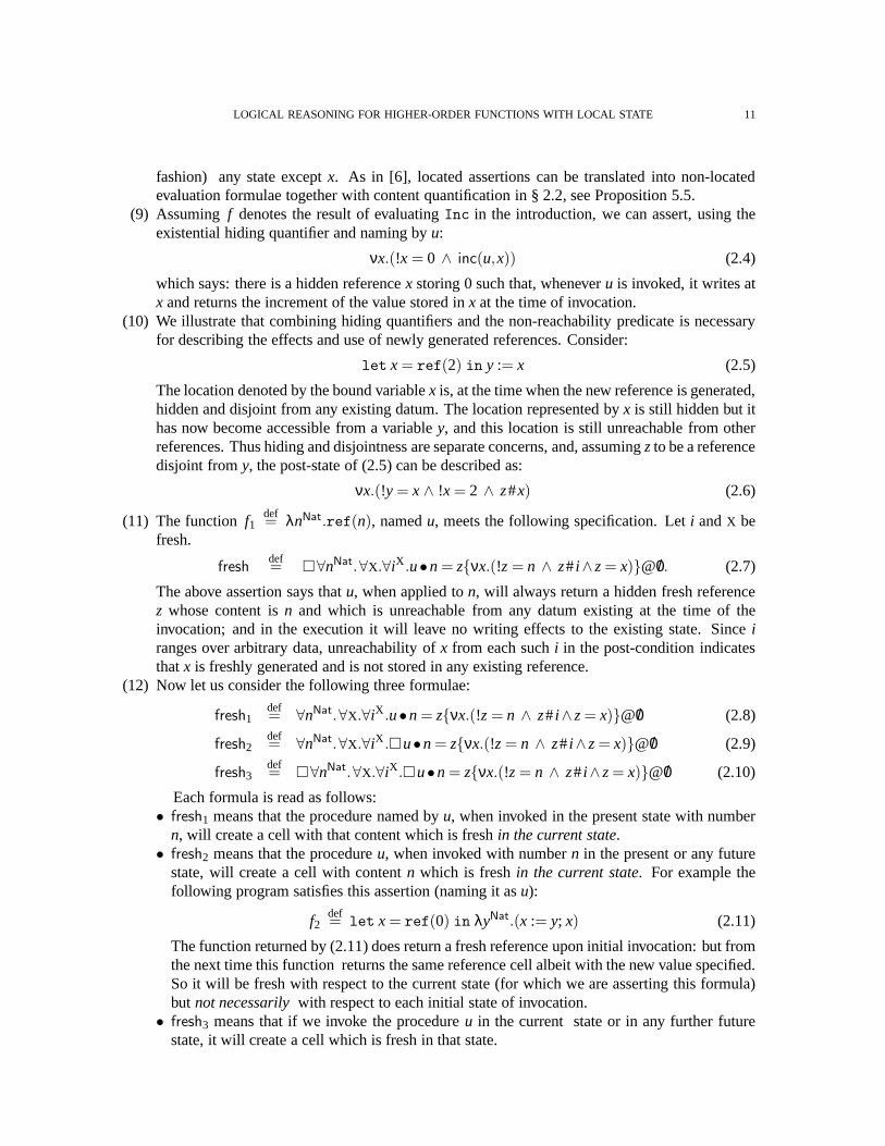
fashion) any state exceptx. As in [6], located assertions can be translated into non-locatedevaluation formulae together with content quantification in § 2.2, see Proposition 5.5.
(9) Assuming f denotes the result of evaluatingInc in the introduction, we can assert, using theexistential hiding quantifier and naming byu:
νx.(!x = 0 ∧ inc(u,x)) (2.4)
which says: there is a hidden referencex storing 0 such that, wheneveru is invoked, it writes atx and returns the increment of the value stored inx at the time of invocation.
(10) We illustrate that combining hiding quantifiers and thenon-reachability predicate is necessaryfor describing the effects and use of newly generated references. Consider:
let x = ref(2) in y := x (2.5)
The location denoted by the bound variablex is, at the time when the new reference is generated,hidden and disjoint from any existing datum. The location represented byx is still hidden but ithas now become accessible from a variabley, and this location is still unreachable from otherreferences. Thus hiding and disjointness are separate concerns, and, assumingzto be a referencedisjoint fromy, the post-state of (2.5) can be described as:
νx.(!y = x∧ !x = 2 ∧ z#x) (2.6)
(11) The functionf1def= λnNat.ref(n), namedu, meets the following specification. Leti andX be
fresh.
freshdef= ∀nNat.∀X.∀iX .u•n = zνx.(!z= n ∧ z#i ∧z= x)@/0. (2.7)
The above assertion says thatu, when applied ton, will always return a hidden fresh referencez whose content isn and which is unreachable from any datum existing at the time of theinvocation; and in the execution it will leave no writing effects to the existing state. Sinceiranges over arbitrary data, unreachability ofx from each suchi in the post-condition indicatesthatx is freshly generated and is not stored in any existing reference.
(12) Now let us consider the following three formulae:
fresh1def= ∀nNat.∀X.∀iX .u•n = zνx.(!z= n ∧ z#i ∧z= x)@/0 (2.8)
fresh2def= ∀nNat.∀X.∀iX .u•n = zνx.(!z= n ∧ z#i ∧z= x)@/0 (2.9)
fresh3def= ∀nNat.∀X.∀iX .u•n = zνx.(!z= n ∧ z#i ∧z= x)@/0 (2.10)
Each formula is read as follows:• fresh1 means that the procedure named byu, when invoked in the present state with number
n, will create a cell with that content which is freshin the current state.• fresh2 means that the procedureu, when invoked with numbern in the present or any future
state, will create a cell with contentn which is freshin the current state. For example thefollowing program satisfies this assertion (naming it asu):
f2def= let x = ref(0) in λyNat.(x := y; x) (2.11)
The function returned by (2.11) does return a fresh reference upon initial invocation: but fromthe next time this function returns the same reference cell albeit with the new value specified.So it will be fresh with respect to the current state (for which we are asserting this formula)but not necessarilywith respect to each initial state of invocation.
• fresh3 means that if we invoke the procedureu in the current state or in any further futurestate, it will create a cell which is fresh in that state.

12 N. YOSHIDA, K. HONDA, AND M. BERGER
Then we have:
fresh ≡ fresh3 ⊃ fresh2 ⊃ fresh1 (2.12)
which we shall prove by the axioms for later. The program (2.11) satisfiesfresh1 andfresh2,but doesnot satisfyfresh (nor fresh3) since f2 returns the same location. On the other hand,f1satisfies all offresh, fresh1, fresh2 andfresh3. This example demonstrates that a combinationof and a decomposed evaluation formula gives precise specifications in the presence of thelocal state.4
3. MODELS AND SEMANTICS
3.1. Models. We introduce the semantics of the logic based on the operational semantics of pro-grams, using partially hidden stores. Our purpose is to havea preciseandclear correspondencebetween programs’ operational behaviour (and the induced observational semantics) and the se-mantics of assertions. This is the reason for defining our models operationally. This approach offersa simple framework to reason about the semantic effects of hidden (and/or newly generated) storeson higher-order imperative programs (for further discussions, see Remark 3.3 later). For capturinglocal state, our models incorporate hidden locations usingν-binders, suggested by theπ-calculus[37]. For example, consider the programInc from the introduction.
Incdef= let x = ref(0) in λ().(x :=!x+1; !x) (3.1)
Recall that after runningInc, we reach a state where a hidden name stores 0, to be used by theresulting procedure when invoked. Hence,Inc namedu, is modelled as:
(νl)(u : λ().(l :=!l +1; !l), l 7→ 0) (3.2)
which says that the appropriate behaviour is atu, in addition to a hidden referencel storing 0.
Definition 3.1. (models) Anopen model of typeΓ is a tuple(ξ,σ) where:
• ξ, calledenvironment, is a finite map from variables indom(Γ) to closed values such that, foreachx∈ dom(Γ), ξ(x) is typed asΓ(x) underΓ, i.e.Γ ⊢ ξ(x) : Γ(x).
• σ, calledstore, is a finite map from labels inl | l ∈ dom(Γ) to closed values such that for eachl ∈ dom(σ), Γ(l) has typeRef(α), thenσ(l) has typeα underΓ, i.e.Γ ⊢ σ(l) : α.
WhenΓ includes free type variables,ξ maps them to closed types, with the obvious correspondingtyping constraints. Amodelof type Γ is a structure(νl)(ξ,σ) with (ξ,σ) being an open model oftypeΓ,∆ with l = dom(∆). (νl) acts as binders.M,M′, . . . range over models.
An open model maps variables and locations to closed values:a model then specifies part of thelocations as “hidden”. For example,(νl)(x : l · y : l ′, [l 7→ 3] · [l ′ 7→ 3]) is a model with a typingenvironment:Γ = x : Ref(Nat),y : Ref(Nat), l ′ : Ref(Nat). We often omitΓ and a mapping fromtype variables to closed types fromM.
Since assertions in the present logic are intended to capture observable program behaviour, thesemantics of the logic uses models quotiented by an observationally sound equivalence, which wechoose to be the standard contextual congruence itself.
4Note that infresh and fresh3, it is essential that we put universal quantifications∀X and ∀iX after . This hasnot been possible in the two-sided evaluation formulae usedin the logics for pure and imperative higher-order functionswithout local state in [6, 22, 24, 25]. See (2.1).

LOGICAL REASONING FOR HIGHER-ORDER FUNCTIONS WITH LOCAL STATE 13
Definition 3.2. AssumeMidef= (νl i)(x : Vi ,σi) typable underΓ. Then we writeM1 ≈ M2 if the
following clause holds for each typed contextC[ · ] which is typable underΓ and in which no labelsfrom l1,2 occur:
(νl1)(C[〈V1〉],σ1) ⇓ iff (νl2)(C[〈V2〉],σ2) ⇓ (3.3)where〈V〉 is then-fold pairings of a vector of values.
Definition 3.2 in effect takes models up to the standard contextual congruence. We could haveused a different program equivalence (for example call-by-value βη convertibility), as far as it isobservationally sound. Note that we have
(νl)(ξ ·x:V1,σ · l 7→W1) ≈ (νl )(ξ ·x:V2,σ · l 7→W2) (3.4)
wheneverV1∼=V2 andW1
∼=W2, where∼= is the contextual congruence on programs defined in § 2.1.To see the reason why we take the models up to observational congruence, let us consider the
following program:
Inc2def= let x = ref(0), y = ref(0) in λ().(x :=!x+1;y :=!y+1; (!x+!y)/2) (3.5)
which is contextually equivalent toInc. Then we have the following model forInc2.
(νll ′)(u : λ().(x :=!x+1;y :=!y+1; (!x+!y)/2), x : l , y : l ′, l 7→ 0, l ′ 7→ 0) (3.6)
Since the two programs originate in the same abstract behaviour, we wish to identify the model in(3.2) and the above model, taking them up to the equivalence.
Remark 3.3. (presentation of models) The model as given above can be presented algebraically us-ing the language of categories [59]. One method, which can treat hiding as above categorically, usesa class of toposes which treat renaming through symmetries [20]. We can also use the “swapping”-based treatment of binding based on [13]. Note however that the use of such different presentations(with respective merits) doesnotalter the equational and other properties of models and the satisfac-tion relation, as far as we wish to use the standard observational semantics (Morris-like contextualcongruence) or the equivalent models (so-called fully abstract models) as a basis of our logic. An-other significant point is that the game-based model in [4] isthe only known model satisfying this(full abstraction) criteria, whose morphisms are isomorphic to a class of typedπ-calculus processes[21]. The presented “operational” model is hinted at by, andis close to, theπ-calculus presentationof semantics of the target language. The present approach allows us to have models which are au-tomatically faithful to the standard observational semantics of the language, directly capturing theeffects of hidden stores by semantics of the logic. Other models may as well be used for exploringvarious aspects of the presented logic.
Remark 3.4. (hidden locations) Following standard textbooks [14, 46],we treat locations as values(which is natural from the viewpoint of reduction). A significant point is that distinctions amongthese values (locations) matter even if they are hidden. Forexample if we have:
Mdef= 〈ref(2),ref(2)〉 (3.7)
and evaluateM, we get a pair of two fresh locations both storing 2. For the denotation of thisresulting value, it is essential that these two references are distinct. For example the program:
Ndef= let x = ref(2) in 〈x,x〉 (3.8)
has a different observable behaviour, as justified by a context C[ ]def= if π1[ ] = π2[ ] then 1 else 2.
Thus distinctions matter, even if locations are hidden.

14 N. YOSHIDA, K. HONDA, AND M. BERGER
3.2. Semantics of Equality. For the rest of this section, we give semantics to assertions, mainlyfocussing on key features concerning local state and which therefore differ from the previous logics[6]. We start with the semantics of equality.
A key example are the programsincShared in (1.2) andincUnShared in (1.3) from theintroduction. After the second assignment of (1.2) and (1.3), we consider whether we can assert“! a = !b” (i.e. the content ofa andb are equal). For this inquiry, let us first recall the followingdefining clause for the satisfaction of equality of two logical terms from [6] which follows thestandard definition of logical equality. First we set, withΓ ⊢ e : α, Γ ⊢ M and an open modelM = (ξ,σ), an interpretation ofeunderM as follows.5
[[x]]ξ,σ = ξ(x) [[!e]]ξ,σ = σ([[e]]ξ,σ) [[c]]ξ,σ = c [[op(e)]]ξ,σ = op([[e]]ξ,σ)
[[〈e,e′〉]]ξ,σ = 〈[[e]]ξ,σ, [[e′]]ξ,σ〉 [[inji(e)]]ξ,σ = inji([[e]]ξ,σ)
which are all standard. Then we define:
(the definition from [6]) M |= e1 = e2def≡ [[e1]]M ≈ [[e2]]M (3.9)
Note that (3.9) says thate1 = e2 is true under an open modelM iff their interpretations inM arecongruent. Now suppose we apply (3.9) to the question of !a = !b in incUnShared. Since the twoinstances ofInc stored ina andb have the identical denotation (or identical behaviour: becausethey are exactly the same programs), the equality !a = !b holds forincUnShared if we use (3.9).However this interpretation is wrong:we observe that, inincUnShared, running !a twice andrunning !a and !b consecutively lead to different observable behaviours, due to their distinct localstates (which can be easily represented using evaluation formulae). Hence we must have !a 6= !b,which says the standard definition (3.9) is not applicable inthe presence of the local state. Onthe other hand, running !a and running !b have always identical observable effects: that is we canalways replace the content ofa with the content ofb in incShared, hence the equality !a = !bshould hold forincShared.
The reason that the standard equality does not hold is because two currently identical statefulprocedures will in future demonstrate distinct behaviour.On the other hand, two identical functionswhich share the same local state always show the same behaviour hence inincShared we obtainequality.
This analysis indicates that we need to consider programs placed in contexts to compare them
precisely, leading to the following extension for the semantics for the equality, assumingMdef=
(νl )(ξ,σ):
M |= e1 = e2def≡ M[u : e1] ≈ M[u : e2] (3.10)
whereM[u : e] denotes(νl )(ξ ·u : [[e]]ξ,σ,σ) with u fresh and the variables and labels ine shouldbe free inM. Note thatM[u : e] offers the notion of a “program-in-context” whene denotes aprogram. For example let us consider a model for the state immediately after the assignmentb :=!ain incShared. Then the model may be written as (takinga andb to be locations):
MincShared = (νl)
/0,a 7→ λ().(l :=!l +1; !l),b 7→ λ().(l :=!l +1; !l),l 7→ n
(3.11)
We obtain (writing the map fora,b, l above asσ for brevity):
MincShared[u :!a] = (νl)(u : λ().(l :=!l +1; !l), σ) (3.12)
5Since a model in [6] does not have local state, it suffices to consider open models.

LOGICAL REASONING FOR HIGHER-ORDER FUNCTIONS WITH LOCAL STATE 15
Notice that the function assigned tou sharesl in the environment: we are interpreting the derefer-ence !a “in context”. Similarly we obtain:
MincShared[u :!b] = (νl)(u : λ().(l :=!l +1; !l), σ) (3.13)
By which we concludeMincShared |=!a =!b: if the results of interpreting two terms in context areequal then we know their effects to the model are equal. We leave it to the reader to check theinequality between !a and !b for the corresponding model representingincUnShared.
The definition of equality above satisfies the standard axioms of equality as we shall see in§ 5. It is also accompanied by a notion ofsymmetrywhich can be used for checking (in)equality,introduced below.
Definition 3.5 (permutation). Let Mdef= (νl )(ξ · v:V ·w:W, σ) whereM is typed underΓ andv,w
have the same type underΓ. Then, we set:
M(vw
wv
) def= (νl )(ξ ·v:W ·w:V, σ) (3.14)
called apermutation ofM at v and w. We extend the notion to an arbitrary bijectionρ ondom(Γ),writing M[ρ]. A permutationρ onM is asymmetry onM whenM[ρ] ≈ M.
Proposition 3.6(symmetries).(1) GivenM1,2 and a bijectionρ on free variables in the domain ofM1,2, we haveM1 ≈ M2 iff
M1[ρ] ≈ M2[ρ].(2) If M1 ≈ M2 andρ is symmetry ofM1, thenρ is symmetry ofM2.
Proof. Obvious by definition. ⊓⊔
We illustrate how we can use the result above to model the subtlety of equality of behaviours withshared local state. Let us consider the following modelsM1 andM2, which represent the situationsanalogous toincShared and incUnShared (again after running the second assignment). Thedefining clause for equality gives , usingM1[u:v] ≈ M1[u:w]:
M1 = (νl)
(
v : λ().(l :=!l +1; !l),w : λ().(l :=!l +1; !l),
l 7→ 0
)
|= v = w (3.15)
On the other hand, we have:
M2 = (νll ′)
(
v : λ().(l :=!l +1; !l),w : λ().(l ′ :=!l ′ +1; !l ′),
l 7→ 0,l ′ 7→ 0
)
|= v 6= w (3.16)
This is because(uv
vu
)
is a symmetry ofM2[u:v], butnot of M2[u:w]. The latter can be examined bycomparing the following two models (writing “u,w : V” to denote “u : V,w : V”):
M2[u:w] = (νll ′)
(
v : λ().(l :=!l +1; !l),u,w : λ().(l ′ :=!l ′ +1; !l ′),
l 7→ 0,l ′ 7→ 0
)
(3.17)
(M2[u:w])(uv
vu
)
= (νll ′)
(
u : λ().(l :=!l +1; !l),v,w : λ().(l ′ :=!l ′ +1; !l ′),
l 7→ 0,l ′ 7→ 0
)
(3.18)
which differ semantically when e.g.v andw are invoked consecutively. Hence by Proposition 3.6(2),M2[u:v] 6≈M2[u:w], justifying the above inequalityv 6= w. The permutations also help to provethe axioms of equality in § 5.
16 N. YOSHIDA, K. HONDA, AND M. BERGER
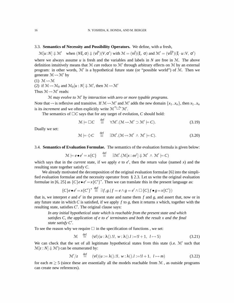
3.3. Semantics of Necessity and Possibility Operators.We define, withu fresh,
M[u:N] ⇓ M′ when(Nξ,σ) ⇓ (νl ′)(V,σ′) with M = (νl)(ξ, σ) andM
′ = (νl l ′)(ξ ·u:V, σ′)
where we always assumeu is fresh and the variables and labels inN are free inM. The abovedefinition intuitively means thatM can reduce toM′ through arbitrary effects onM by an externalprogram: in other words,M′ is a hypothetical future state (or “possible world”) ofM. Then wegenerateM M′ by
(1) M M
(2) if M M0 andM0[u : N] ⇓ M′, thenM M′
ThusM M′ reads:
M may evolve toM′ by interaction with zero or more typable programs.
Note that is reflexive and transitive. IfM M′ andM′ adds the new domainx1..xn, thenx1..xn
is its incrementand we often explicitly writeMx1..xn M′.
The semantics ofC says that for any target of evolution,C should hold:
M |=Cdef≡ ∀M
′.(M M′ ⊃ M
′ |= C). (3.19)
Dually we set:
M |= ♦Cdef≡ ∃M
′.(M M′ ∧ M
′ |= C). (3.20)
3.4. Semantics of Evaluation Formulae.The semantics of the evaluation formula is given below:
M |= e•e′ = xCdef≡ ∃M
′.(M[x : ee′] ⇓ M′ ∧ M
′ |= C)
which says that in thecurrent state, if we applye to e′, then the return value (namedx) and theresulting state together satisfyC.
We already motivated the decomposition of the original evaluation formulae [6] into the simpli-fied evaluation formulae and the necessity operator from § 2.3. Let us write the original evaluationformulae in [6, 25] asCe•e′=xC′⋆. Then we can translate this in the present language as:
Ce•e′=xC′⋆ def≡ ∃ f ,g.( f = e∧g = e′∧C f •g=xC′)
that is, we interprete ande′ in the present state and name themf andg, and assert that, now or inany future state in whichC is satisfied, if we applyf to g, then it returnsx which, together with theresulting state, satisfiesC′. The original clause says:
In any initial hypothetical state which is reachable from the present state and whichsatisfies C, the application of e to e′ terminates and both the result x and the finalstate satisfy C′.
To see the reason why we require in the specification of functions , we set:
Mdef= (νl)(u : λ().!l , w : λ().l :=!l +1, l 7→ 5) (3.21)
We can check that the set of all legitimate hypothetical states from this state (i.e.M′ such thatM[z : N] ⇓ M′) can be enumerated by:
M′/z
def= (νl)(u := λ().!l , w : λ().l :=!l +1, l 7→ m) (3.22)
for eachm≥ 5 (since these are essentially all the models reachable fromM , as outside programscan create new references).

LOGICAL REASONING FOR HIGHER-ORDER FUNCTIONS WITH LOCAL STATE 17
Thus we have, forM in (3.21):
M |=w• () = xx≥ 5 (3.23)
which says in anyfuturestate wherew is invoked, it always returns something no less than 5, whichis operationally reasonable.
We can use this formula for specifying the following program:
Ldef= let x = ref(5) in
let u = λ().!x inlet w = λ().x :=!x+1 in
( f w) ; if x≥ 5 then t else f
(3.24)
When the applicationf w takes place, some unknown computation occurs which may change thevalue ofx: but as far asf w terminates, it always returnst. To reach (3.23), we need to considerallpossibleM′ with the effect from the outside. Since suchM′ satisfies (3.22), we can conclude theprogramL always returnst (if f w terminates).
3.5. Semantics of Universal and Existential Quantification.The universal and existential quan-tifiers also need to incorporate local state. We need one definition to identify a set of terms whichdo not change the state of any models. BelowMΓ indicates thatM is typable underΓ.
Definition 3.7 (Functional Terms). We define the set offunctional termsof typeΓ, denotedFΓ, oroften simplyF leaving its typing implicit, as:
Fdef= N | ∀M
Γ.(M[u : N] ⇓ M′ ⊃ M ∼= M
′/u)
whereM/udef= (νl)(ξ,σ) if M = (νl)(ξ ·u:V,σ); andM/u
def= M whenu 6∈ fv(M). We writeL,L′, ...
for functional terms, often leaving their types implicit.
AboveM ∼= M′/u ensures thatL does not affectM during evaluation ofL in M. Note that valuesare always functional terms. In a context of reasoning for object-oriented languages, a similarformulation (called strong purity) is used in [44] for justifying the semantics of method invocationswhose evaluation has no effect on the state of existing objects.
Now we define:
M |= ∀x.Cdef≡ ∀L ∈ F.(M[x:L] ⇓ M
′ ⊃ M′ |= C) (3.25)
Dually, we have:
M |= ∃x.Cdef≡ ∃L ∈ F.(M[x:L] ⇓ M
′ ∧ M′ |= C) (3.26)
If we restrict L above to a value, then the definition coincides with the original one in [6]. Weneed to extend values to functional terms so that a term can read information from hidden locations(cf. the semantics of equalitye1 = e2). As a simple example, consider:
Mdef= (νl1, l2)(y : l1, l1 7→ l2, l2 7→ 2)
Under this model, we wish to sayM |= ∃x.x =!y. But if we only allowx to range over values, thisstandard tautology does not hold forM. Using the functional term !y∈ F, we can expand the entryx with !y, and we have:
M[x : !y] ⇓ (νl1l2)(x : l1 ·y : l1, l1 7→ l2, l2 7→ 2)def= M
′ ∧ M′ |= x = y

18 N. YOSHIDA, K. HONDA, AND M. BERGER
Thus using a functional termL instead of a valueV for a quantified variable is necessary for rea-sons similar to those that required modifying the semanticsof equality. Universal and existentialquantifiers satisfy the standard axioms familiar from first-order logic, some of which are studiedlater.
3.6. Semantics of Hiding. The universal hiding-quantifier has the following semantics.
M |= νx.Cdef≡ ∀M
′.((νl)M′ ≈ M ⊃ M′[x : l ] |= C) (3.27)
wherel is fresh, i.e.l 6∈ fl(M) wherefl(M) denotes free labels inM. The notation(νl)M′ denotesaddition of the hiding ofl to M′, as well as indicating thatl occurs free inM′. M[x : l ] addsx : l tothe environment part ofM.
Dually, with l fresh again:
M |= νx.Cdef≡ ∃M
′.((νl)M′ ≈ M ∧ M′[x : l ] |= C) (3.28)
which says thatx denotes a hidden reference, sayl , and the result of taking it off fromM satisfiesC.
As an example of satisfaction, let:
Mdef= (νl)(u : λ().(l :=!l +1; !l), l 7→ 0) (3.29)
then we have:M |= νx.C (3.30)
withC
def= !x = 0 ∧ ∀i.!x = iu• () = zz=!x∧ !x = i +1 (3.31)
using the definition in (3.28) above. To see this holds, let
M′ def= (u : λ().(l :=!l +1; !l), l 7→ 0) (3.32)
We have(νl)M′ def≡ M andM′[x : l ] |= C. HereM represents a situation wherel is hidden andu
denotes a function which increments and returns the contentof l ; whereasM′ is the result of takingoff this hiding, exposing the originally local state, cf. [11].
Despitex’s type being a reference,∀x.C differs substantially fromνx.C. The former says thatfor any referencex, which can be either (1) an existing free reference; (2) an existing hidden ref-erence reachable through dereferences; or (3) a fresh reference with arbitrary content, the modelsatisfiesC. On the other hand, the latter means that for any referencex which is hidden in thepresent model,C should hold: in this casex cannot be a free reference name hence (1) is not in-cluded. Similarly for their dual existential versions.
3.7. Semantics of Content Quantification. Next we define the semantics of the content quantifi-cation. Let us writeM[x 7→ V] for (νl)(ξ,σ[l 7→ V]) with M = (νl)(ξ,σ) and ξ(x) = l . In [6](without local state),M |= [!x]C is defined as∀V.M[x 7→ V] |= C which means that for all contentof x, C holds. In the presence of the local state, we simply extend the use of values to the use offunctional terms in the sense of Definition 3.7 as follows:
M |= [!e]Cdef≡ ∀L ∈ F.M[e 7→ L] |= C (3.33)

LOGICAL REASONING FOR HIGHER-ORDER FUNCTIONS WITH LOCAL STATE 19
where we writeM[e 7→ L] for (νl )(ξ,σ[l ′ 7→V]), assumingM = (νl)(ξ,σ), [[e]]ξ,σ = l ′, (νl)(Lξ,σ)⇓
M′ andM′ ≈ (νl)(V,σ). Thus we consider an update through the assignment of an external func-tional termL to a location inM under local names. With this definition, all the axioms and invariantrules in [6] stay unchanged.
3.8. Semantics of Reachability.We now define the semantics of reachability. Letσ be a store andS⊂ dom(σ). Then thelabel closure of S inσ, written lc(S,σ), is the minimum setS′ of locationssuch that: (1)S⊂ S′ and (2) If l ∈ S′ thenfl(σ(l)) ⊂ S′. The label closure satisfies the followingnatural properties.
Lemma 3.8. For all σ, we have:
(1) S⊂ lc(S,σ); S1 ⊂ S2 implieslc(S1,σ) ⊂ lc(S2,σ); and lc(S,σ) = lc(lc(S,σ),σ)(2) lc(S1,σ)∪ lc(S2,σ) = lc(S1∪S2,σ)(3) S1 ⊂ lc(S2,σ) and S2 ⊂ lc(S3,σ), then S1 ⊂ lc(S3,σ)(4) there existsσ′ ⊂ σ such thatlc(S,σ) = fl(σ′) = dom(σ′).
Proof. (1,2) are direct from the definition. (3) follows immediately from (1,2). For (4), takeσ′ =∪l∈lc(S,σ)[l 7→ σ(l)]. Then obviouslyσ′ ⊂ σ andlc(S,σ) = fl(σ′) = dom(σ′). ⊓⊔
For reachability, we define:
M |= e1 → e2 if [[e2]]ξ,σ ∈ lc(fl([[e1]]ξ,σ),σ) for each(νl)(ξ,σ) ≈ M
The clause says the set of all reachable locations frome1 includese2 modulo≈.For the programs in § 2.3 (5), we can checkfw → x, fr → x and fc → zhold underfw : λ().(x :=
1), fr : λ().!x, fc : let x = ref(z) in λ().x (regardless of the store part).The following characterisation of # is often useful for justifying fresh name axioms. Below
σ = σ1⊎σ2 indicates thatσ is the union ofσ1 andσ2, assumingdom(σ1)∩dom(σ2) = /0.
Proposition 3.9(partition). M |= x#u if and only if for somel, V , l andσ1,2, we haveM≈ (νl )(ξ ·u :V ·x : l , σ1⊎σ2) such thatlc(fl(V),σ1⊎σ2) = fl(σ1) = dom(σ1) and l∈ dom(σ2).
Proof. For the only-if direction, assumeM |= x#u. By the definition of (un)reachability, we can set
(up to≈) Mdef= (νl ′)(ξ ·u :V ·x : l , σ) such thatl 6∈ lc(fl(V),σ). Now takeσ1 such thatlc(fl(V),σ) =
lc(fl(V),σ1) = fl(σ1) = dom(σ1) by Lemma 3.8. Note by definitionl 6∈ dom(σ1). Now let σ =σ1 ⊎σ2. Sincel ∈ dom(σ), we know l ∈ dom(σ2), hence done. The if-direction is obvious bydefinition of reachability. ⊓⊔
The characterisation says that ifx is unreachable fromu then, up to≈, the store can be partitionedinto one covering all reachable names fromu and another containingx.
Now we give the full definition of the satisfaction relation.For readability, we first list theauxiliary definitions many of which have already been statedbefore.
Notation 3.10.(a) M[u:e] denotes(νl )(ξ ·u : [[e]]ξ,σ,σ) where we always assumeu is fresh and the variables and
labels ineare free inM.(b) M/u denotes(νl)(ξ,σ) if M = (νl)(ξ ·u:V,σ); and ifu 6∈ fv(M) we setM/u = M.(c) M[u : N] ⇓ M′ when(Nξ,σ) ⇓ (νl ′)(V,σ′) andM′ = (νl l ′)(ξ · u :V, σ′) with M = (νl )(ξ, σ)
where we always assumeu is fresh and the variables and labels inN are free inM.(d) M M′ is generated by: (1)M M; and (2) ifM M0 andM0[u : N] ⇓ M′, thenM M′.
20 N. YOSHIDA, K. HONDA, AND M. BERGER
(e) We writeM[e 7→V] for (νl )(ξ,σ[l 7→V]) with M = (νl)(ξ,σ) and[[e]]ξ,σ = l .(f) We write M·X : α for M = (νl)(ξ·X : α,σ) with M = (νl)(ξ,σ) whereX is not inM andα is
closed.
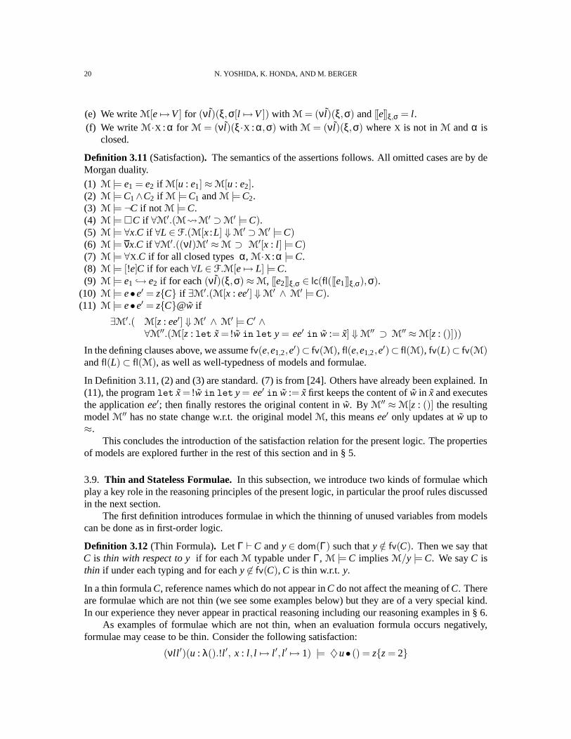
Definition 3.11 (Satisfaction). The semantics of the assertions follows. All omitted cases are by deMorgan duality.
(1) M |= e1 = e2 if M[u : e1] ≈ M[u : e2].(2) M |= C1∧C2 if M |= C1 andM |= C2.(3) M |= ¬C if not M |= C.(4) M |=C if ∀M′.(M M′ ⊃ M′ |= C).(5) M |= ∀x.C if ∀L ∈ F.(M[x:L] ⇓ M′ ⊃ M′ |= C)(6) M |= νx.C if ∀M′.((νl)M′ ≈ M ⊃ M′[x : l ] |= C)(7) M |= ∀X.C if for all closed typesα, M·X :α |= C.(8) M |= [!e]C if for each∀L ∈ F.M[e 7→ L] |= C.(9) M |= e1 → e2 if for each(νl)(ξ,σ) ≈ M, [[e2]]ξ,σ ∈ lc(fl([[e1]]ξ,σ),σ).
(10) M |= e•e′ = zC if ∃M′.(M[x : ee′] ⇓ M′ ∧ M′ |= C).(11) M |= e•e′ = zC@w if
∃M′.( M[z : ee′] ⇓ M′ ∧ M′ |= C′ ∧∀M′′.(M[z : let x = !w in let y = ee′ in w := x] ⇓ M′′ ⊃ M′′ ≈ M[z : ()]))
In the defining clauses above, we assumefv(e,e1,2,e′)⊂ fv(M), fl(e,e1,2,e′)⊂ fl(M), fv(L)⊂ fv(M)andfl(L) ⊂ fl(M), as well as well-typedness of models and formulae.
In Definition 3.11, (2) and (3) are standard. (7) is from [24].Others have already been explained. In(11), the programlet x= !w in let y= ee′ in w := x first keeps the content of ˜w in x and executesthe applicationee′; then finally restores the original content in ˜w. By M′′ ≈ M[z : ()] the resultingmodelM′′ has no state change w.r.t. the original modelM, this meansee′ only updates at ˜w up to≈.
This concludes the introduction of the satisfaction relation for the present logic. The propertiesof models are explored further in the rest of this section andin § 5.
3.9. Thin and Stateless Formulae.In this subsection, we introduce two kinds of formulae whichplay a key role in the reasoning principles of the present logic, in particular the proof rules discussedin the next section.
The first definition introduces formulae in which the thinning of unused variables from modelscan be done as in first-order logic.
Definition 3.12 (Thin Formula). Let Γ ⊢C andy∈ dom(Γ) such thaty /∈ fv(C). Then we say thatC is thin with respect to yif for eachM typable underΓ, M |= C impliesM/y |= C. We sayC isthin if under each typing and for eachy 6∈ fv(C), C is thin w.r.t.y.
In a thin formulaC, reference names which do not appear inC do not affect the meaning ofC. Thereare formulae which are not thin (we see some examples below) but they are of a very special kind.In our experience they never appear in practical reasoning including our reasoning examples in § 6.
As examples of formulae which are not thin, when an evaluation formula occurs negatively,formulae may cease to be thin. Consider the following satisfaction:
(νll ′)(u : λ().!l ′, x : l , l 7→ l ′, l ′ 7→ 1) |= ♦u• () = zz= 2

LOGICAL REASONING FOR HIGHER-ORDER FUNCTIONS WITH LOCAL STATE 21
which means thatu is a function which might return 2somedaysince a value stored inl ′ can bechanged viax (for example, by the command !x := 2). When we deletex from the above model, thebehaviour ofu will change as follows.
(νl ′)(u : λ().!l ′, l ′ : 1) |= u• () = zz= 1
since nowu alwaysreturns 1 when it is invoked. The above judgement entails:
(νl ′)(u : λ().!l ′, l ′ : 1) 6|= ♦u• () = zz= 2
Hence♦u• () = zz= 2 is not thin. Similarly♦u• () = zz= 0 is not a thin formula.As noted, formulae which are not thin hardly appear in reasoning; all formulae appearing in § 6
are thin; the proof rules always generate thin formulae fromthin formulae. We shall however workwith general formulae since many results hold for none-thinformulae too.
The following syntactic characterisation of thin formulaeis useful.
Proposition 3.13(Syntactically Thin Formula). (1) If Γ ⊢C, Γ ⊢ y : α andα ∈ Unit,Bool,Nat,then C is thin with respect to y.
(2) e= e′,e 6= e′,e → e′ and e#e′ are thin.(3) If C,C′ are thin w.r.t. y, then C∧C′, C∨C′, ∀xα.C for all α, ∃xα.C with α ∈ Unit,Bool,Nat,
∃X.C,∀X.C, νx.C, νx.C,C, [!x]C and e•e′ = xC′ are thin w.r.t. y.
Proof. (1,2) are immediate. For (3), supposeC andC′ are thin w.r.t.y, y 6∈ fv(C,C′) andM |=C∧C′.ThenM |=C henceM/y |=C, similarly forC′, henceM/y |=C∧C′. Similarly for other cases. Nextlet C be thin w.r.t.y andM |= νx.C. Then there existsM′ such that(νl)M′ ≈ M andM′[x : l ] |= C.Then(νl)M′/y≈ M/y. By assumption,M′[x : l ]/y |= C, and henceM/y |= νx.C, as desired. Nextlet C be thin w.r.t.y. SupposeM |= e•e′ = zC, i.e. M[z : ee′] ⇓ M′ andM′ |= C. Then we haveM/y[z : ee′] ⇓ M′/y. SinceC is thin w.r.t.y, we haveM′/y |= C, as required. ⊓⊔
The next set of formulae arestateless formulaewhose validity does not depend on the state partof the model, cf. stateless formulae in [6, 25].
Definition 3.14 (Stateless Formula). C is statelessiff C ⊃C is valid. We letA,B,A′,B′, . . . rangeover stateless formulae.
Proposition 3.15(Stateless Formulae). (1) For all C,C is stateless.(2) If C is stateless then C≡C≡C.
Proof. Both are immediate from the definition, see also § 5.2 for further related results. ⊓⊔
The above proposition says that ifC is stateless thenC holds in any future state starting from thepresent state. The following generalisation of this notionsays that the validity of a formula does notdepend on the stateful part of modelsexcept at specific locations. This notion is used by the axiomsfor local invariants later.
Definition 3.16 (Stateless Formula Except ˜x). We say thatC is stateless exceptx if, wheneverM |= C andM M′ such thatM andM′ coincide in their content at ˜x of reference types, i.e.
(1) M ≈ (νl0)(ξ, σ);(2) M′ ≈ (νl0l1)(ξ ·ξ′, σ′); and(3) σ(ξ(xi)) = σ′(ξ(xi)) for eachxi ∈ x,thenM′ |= C.

22 N. YOSHIDA, K. HONDA, AND M. BERGER
Definition 3.16 uses the internal representation of models.Alternatively we may define an ˜x-preserving termwhich has the shape:
let y1 = !x1 in ...let yn = !xn in let z= N′ in (x1 := y1; ...;xn := yn;z) (3.34)
then sayC is stateless except ˜x if wheneverM |= C andM[u : N] ⇓ M′ whereN is a x-preservingterm we haveM′ |= C.
Note if x is empty in Definition 3.16 then the third clause is vacuous: hence in this case thedefinition means that for eachM such thatM |= C we haveM M′ impliesM′ |= C, that isC isstateless.
It is convenient to be able to check the statelessness of formulae (relative to references) syntac-tically. For an inductive characterisation, we introduce the following notion. As always we assumethe standard bound name convention.
Definition 3.17 (Tame Formulae). The set oftame formulaeis generated by the following rules:
• e1 = e2 ande1 6= e2 are tame.• e1 → e2 ande1 #e2 are tame.• For anyC,C is tame.• if C is tame then∀yα.C, ∃yα.C, ∃X.C, ∀X.C, [!y]C and〈!y〉C are all tame.• if C,C′ are tame thenC∧C′ andC∨C′ are tame.
We say that !x is anactive dereferencein C if C is tame and !x (with x being free or bound) occursneither in the scope of , [!x] nor 〈!x〉.
The following result (though not used in the present work) isnotable for carrying over reasoningtechniques from the logic for aliasing [6].
Proposition 3.18(Decomposition). Suppose C is tame. Then there is tame C′ such that C≡C′ andC′ does not contain content quantifications except under the scope of .
Proof. The proof follows precisely that of [6, §6.1, Theorem 1]. ⊓⊔
We can now introduce syntactic stateless formulae.
Definition 3.19 (Syntactic Stateless Formulae). We sayC is syntactically stateless exceptx if C istame and only names from ˜x are among the active dereferences inC.
Proposition 3.20.(1) If C is syntactically stateless exceptx then C is stateless exceptx.(2) If [!x]C is syntactically stateless then C is stateless exceptx.
Proof. (1) is by induction of the generation of tame formulae. Base cases andC are immediate.Among the inductive cases the only non-trivial case is quantifications of references. SupposeC istame and contains active dereferences at ˜xy.• If the validity of C relies ony (i.e. for someM1,2 which differ only aty we haveM1 |= C and
M2 6|= C) then∀yα.C is falsity: if not ∀yα.C andC are equivalent. In either case we knowC isstateless except ˜x.
• If validity of C relies ony then∃yα.C is truth: if not∃yα.C andC are equivalent. The rest is thesame.
• If validity of [!y]C relies on the content ofy then[!y]C is falsity: the rest is the same. Similarlyfor 〈!y〉C.
The cases ofC∧C′ andC∨C′ are immediate by induction. (2) is an immediate corollary of(1). ⊓⊔
LOGICAL REASONING FOR HIGHER-ORDER FUNCTIONS WITH LOCAL STATE 23
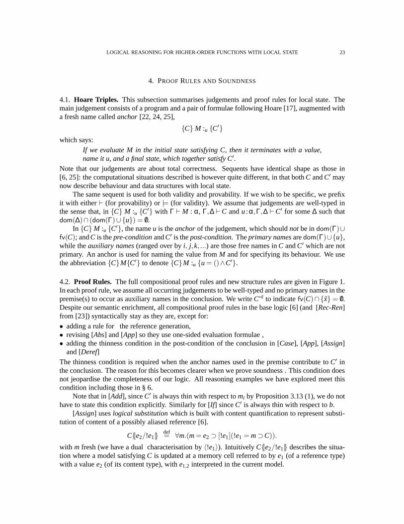
4. PROOF RULES AND SOUNDNESS
4.1. Hoare Triples. This subsection summarises judgements and proof rules for local state. Themain judgement consists of a program and a pair of formulae following Hoare [17], augmented witha fresh name calledanchor[22, 24, 25],
C M :u C′
which says:
If we evaluate M in the initial state satisfying C, then it terminates with a value,name it u, and a final state, which together satisfy C′.
Note that our judgements are about total correctness. Sequents have identical shape as those in[6, 25]: the computational situations described is howeverquite different, in that bothC andC′ maynow describe behaviour and data structures with local state.
The same sequent is used for both validity and provability. If we wish to be specific, we prefixit with either⊢ (for provability) or |= (for validity). We assume that judgements are well-typed inthe sense that, inC M :u C′ with Γ ⊢ M : α, Γ,∆ ⊢C andu:α,Γ,∆ ⊢C′ for some∆ such thatdom(∆)∩ (dom(Γ)∪u) = /0.
In C M :u C′, the nameu is theanchorof the judgement, which shouldnot be indom(Γ)∪fv(C); andC is thepre-conditionandC′ is thepost-condition. Theprimary namesaredom(Γ)∪u,while theauxiliary names(ranged over byi, j,k, ...) are those free names inC andC′ which are notprimary. An anchor is used for naming the value fromM and for specifying its behaviour. We usethe abbreviationCMC′ to denoteCM :u u = ()∧C′.
4.2. Proof Rules. The full compositional proof rules and new structure rules are given in Figure 1.In each proof rule, we assume all occurring judgements to be well-typed and no primary names in thepremise(s) to occur as auxiliary names in the conclusion. Wewrite C-x to indicatefv(C)∩x = /0.Despite our semantic enrichment, all compositional proof rules in the base logic [6] (and [Rec-Ren]from [23]) syntactically stay as they are, except for:
• adding a rule for the reference generation,• revising [Abs] and [App] so they use one-sided evaluation formulae ,• adding the thinness condition in the post-condition of the conclusion in [Case], [App], [Assign]
and [Deref]
The thinness condition is required when the anchor names used in the premise contribute toC′ inthe conclusion. The reason for this becomes clearer when we prove soundness . This condition doesnot jeopardise the completeness of our logic. All reasoningexamples we have explored meet thiscondition including those in § 6.
Note that in [Add], sinceC′ is always thin with respect tomi by Proposition 3.13 (1), we do nothave to state this condition explicitly. Similarly for [If] sinceC′ is always thin with respect tob.
[Assign] useslogical substitutionwhich is built with content quantification to represent substi-tution of content of a possibly aliased reference [6].
C|e2/!e1|def= ∀m.(m= e2 ⊃ [!e1](!e1 = m⊃C)).
with m fresh (we have a dual characterisation by〈!e1〉). Intuitively C|e2/!e1| describes the situa-tion where a model satisfyingC is updated at a memory cell referred to bye1 (of a reference type)with a valuee2 (of its content type), withe1,2 interpreted in the current model.

24 N. YOSHIDA, K. HONDA, AND M. BERGER
[Var] −C[x/u] x :u C
[Const] −C[c/u] c :u C
[Add]CM1 :m1 C0 C0M2 :m2 C′[m1 +m2/u]
CM1 +M2 :u C′
[In1]C M :v C′[inj1(v)/u]C inj1(M) :u C
′[Case]
C-x M :m C-x0 C0[inji(xi)/m] Mi :u C′ -x
C case M of ini(xi).Mii∈1,2 :u C
′
[Proj1]C M :m C′[π1(m)/u]
C π1(M) :u C′[Pair]
C M1 :m C0 C0 M2 :n C′[〈m,n〉/u]
C 〈M1,M2〉 :u C′
[Abs]A-xi ∧C M :m C′
A λx.M :u ∀xi.(Cu• x= mC′)[App]
C M :m C0 C0 N :n m•n= uC′
C MN :u C′
[If ]C M :b C0 C0[t/b] M1 :u C
′ C0[f/b] M2 :u C′
C if M then M1 else M2 :u C′
[Deref]C M :m C′[!m/u]
C !M :u C′[Assign]
C M :m C0 C0 N :n C′|n/ !m|C M := N C′
[Rec-Ren]A- f λx.M :u B
A µ f.λx.M :u B[u/ f ][Ref]
C M :m C′
C ref(M) :u νx.(C′[!u/m]∧u#iX ∧u = x)
[Aux∀V]C-i V :u C′C V :u ∀i.C′
[Aux∀]C-i M :u C′ α is base type
C M :u ∀iα.C′
[Conseq]C⊃C0 C0M :uC
′0C′
0 ⊃C′
C M :u C′[Subs]
C M :u C′ u 6∈ fpn(e)C[e/i] M :u C′[e/i]
[Cons-Eval]
C0 M :m C′0 x fresh; i auxiliary
∀X.∀i.C0x• ()=mC′0 ⊃ ∀X.∀i.Cx• ()=mC′
C M :m C′
We requireC′ is thin w.r.t.m in [Case] and [Deref], andC′ is thin w.r.t.m,n in [App, Assign].
Figure 1: Proof Rules
In rule [Ref], u#i indicates that the newly generated cellu is unreachable from anyi of arbitrarytypeX in the initial state: then the result of evaluatingM is stored in that cell.6 Herei is a(ny) freshvariable denoting an arbitrary datum which already exited in the pre-state. Just as the standardauxiliary variable in Hoare-like logics, thisi is semantically bound at the sequent level. In a largeproof, we may want each instance of [Ref] to use a fresh and distinct variable, even though inpractice we usually apply the substitution rule discussed below to instantiate this “bound” variableinto an appropriate expression so name clash may not occur.7
For the structural rules (i.e. those which only manipulate assertions), those given in [6, §7.3]for the base logic stay valid except that the universal abstraction rule[Aux∀] in [6, §7.3] needs tobe weakened as[Aux∀] and[Aux∀V] in Figure 1. Note that the original structural rule[Aux∀], whichdoes not have this condition, is not valid in the presence of new reference generation. For examplewe can take:
T ref(3) :u u#i∧!u = 3 (4.1)
6One may write the conclusion of this rule asC ref(M) :u (C′[!u/m]∧u#iX ) which may be useful for readability.In this paper however we intentionally do not introduce thisor other abbreviations for the sake of clarity.
7The treatment of a fresh variable as an input binder in [Ref] is useful for mechanisation of reasoning, just like auxiliaryvariables in Hoare triples.

LOGICAL REASONING FOR HIGHER-ORDER FUNCTIONS WITH LOCAL STATE 25
which is surely valid. But without the side condition, we caninfer the following from (4.1).
T ref(3) :u ∀i.(u#i∧!u = 3)
which does not make sense (just substituteu for i). This is becausei cannot range over newlygenerated names: such an interplay with new name generationis not possible if the target programis a value, or ifi is of base type.
We also have two useful structural rules added in the presentlogic. The first rule is [Subs] inFigure 1, which can be used to instantiate the fresh variablei in [Ref] with an arbitrary datum. Therule uses the following set of reference names.
Definition 4.1 (Plain Name). We write fpn(e) for the set offree plain namesof e, defined as:fpn(x) = x, fpn(c) = fpn(!e) = /0, fpn(〈e,e′〉) = fpn(e)∪ fpn(e′), andfpn(inji(e)) = fpn(e).
In brief, the set of free plain names ofecontains reference names inethat do not occur dereferenced,as first described in Definition 4.1. As we shall see later, theside condition for [Subs] using fpn(e)is necessary for soundness.
As an example usage of [Subs], consider:
!z= 2ref(2) :m !m= 2∧ i #m (4.2)
where we take offν by an axiom later. We can then use [Subs] to show:
!z= 2ref(2) :m !m= 2∧z#m (4.3)
Note m∈ fpn(m): hence wecannotusem instead ofz in (4.3), which is obviously unsound. Asanother use of [Subs], consider a judgement:
T〈ref(2),ref(2)〉 :m !π1(m) = 2∧!π2(m) = 2∧π1(m) 6= π2(m) (4.4)
In order to derive (4.4), we simply combine (4.2) with the following judgement:
!m= 2∧ i #mref(2) :n !m= 2∧!n = 2∧ j #n (4.5)
where we use a different fresh variablej. We can now replacej with musing [Subs], and via [Cons]we obtain:
!m= 2∧ i #mref(2) :n !m= 2∧!n = 2∧m 6= n (4.6)from which we can infer (4.4) by pairing, combined with (4.2).
Another significant additional rule is [Cons-Eval], also given in Figure 1. This is a strengthenedversion of the standard consequence rule, and is used when incorporating the local invariant axiomof the evaluation formula for derivations of the examples in§ 6. Technically, this is a consequenceof (a) having a proof system by which we can compositionally build proofs; and (b) representingfresh generation of references by disjointness from fresh variables. We shall see in examples that itis useful in reasoning.
The full list of structural rules can be found in Appendix B.
4.3. Located Judgements.Proof rules which contain an explicit effect set (similar tolocated eval-uation formulae) were introduced in [6] and are of substantial help in reasoning about programs.Located Hoare triples take the form:
CM :uC′@e

26 N. YOSHIDA, K. HONDA, AND M. BERGER
where eachei is of a reference type and does not contain (sub)expressionsof the form !g .8 e iscalledeffect set. We prefix it with either⊢ (for provability) or |= (for validity) if we wish to bespecific.
The full rules are listed in Figure 4 (proof rules) and Figure5 (structure rules) in Appendix B.All rules come from [6] except for the new name generation rule and the universal quantificationrule, both corresponding to the new rules in the basic proof system. The structures rules are alsorevised along the lines of Figure 1.
4.4. Invariance Rules for Reachability. Invariance rules are useful for modular reasoning. Asimple form is when there is no state change:
[Inv-Val]CV :m C′
C∧C0V :m C′∧C0
Alternatively if a formula is stateless it continues to holdirrespective of state change.
[Inv-Stateless]C M :m C′
C∧C0 M :m C′∧C0
When it is formulated with (un)reachability predicates, however, one needs some care. Since reach-ability is a stateful property, it is generallynot invariant under state change. For example, supposexis unreachable fromy; after runningy := x, x becomes reachable fromy. Hence the following ruleis unsound.
[Unsound-Inv]C M :m C′
C∧e#e′ M :m C′∧e#e′(unsound)
From the following general invariance rule [Inv], we can derive an invariance rule for #.
[Inv]C M :m C′@w C0 is tameC∧ [!w]C0 M :m C′∧ [!w]C0@w
In [Inv], the effect set ˜w gives the minimum information by which the assertion we wishto add,C0,can be stated as an invariant since[!w]C0 says thatC0 holds regardless of the content of ˜w. ThusC0 can stay invariant after execution ofM. Unlike the existing invariance rules as found in standardHoare logic or in Separation Logic [56], we need no side condition “M does not modify storesmentioned inC0”: C andC0 may even overlap in their mentioned references, andC does not haveto mention all referencesM may read or write.
The following instance of [Inv] is useful.
[Inv-#]C M :m C′@x no dereference occurs in ˜e
C∧x#e M :m C′∧x#e@x
In [Inv-#], we note[!x]x#e≡ x#e is always valid ifecontains no dereference !e, cf. Proposition 5.93-(5) later. Hencex#e is stateless except atx. The side condition is indispensable: considerTx :=xT@x (which is typable with recursive types), which does not imply x#!xx := xx#!x@x.
One of the important aspects of these invariance rules is that the effect set of a located judge-ment or assertion can contain a hidden name – a name which has been created and which is (par-tially) accessible. For example, we can infer (using[LetRef] in § 6.1):9
!y = h let x = ref(2) in !y = x :u νx.(!h = x∧!x = 2∧!y = h∧x#i)@h
8 This restriction is for a simplification of the interpretation, and can be taken off if ˜e is interpreted in the pre-condition.9Since !y is stated in the pre-condition, we can also writeT let x = ref(2) in !y = x :u νx.(!x = 2∧!!y =
x∧x#i)@!y, cf. footnote 8.
LOGICAL REASONING FOR HIGHER-ORDER FUNCTIONS WITH LOCAL STATE 27
4.5. Soundness.Let M be a model(νl)(ξ,σ) of typeΓ, andΓ ⊢ M : α with u fresh. Thenvalidity|= CM :u C′ is given by (withM including all variables inM, C andC′ exceptu):
|= CM :u C′
def≡ ∀M.(M |= C ⊃ (M[u:M] ⇓ M
′ ∧ M′ |= C′))
where the notationM[u: N] ⇓ M′ appeared in Definition 3.11(c). This is equivalent to, withVdef=
λ().M:∀M.(M[m : V] |=Cm• ()=uC′) (4.7)
Similarly the semantics of the located judgement:
|= C M :u C′@x (4.8)
is given through the corresponding located assertion, using the following term (letzbe fresh):
Vdef= let z= ref(0) in λ().if !z= 0 then let m= M in (z :=!z+1;m) else Ω (4.9)
whereΩ is a diverging closed term (in fact any closed program works). The use ofz is to pre-vent leakage of information fromm after the evaluation: after evaluationm can never reveal anyinformation thus it is the same thing as evaluatingM once.
With thisV we set the definition of (4.8) as follows:
∀M.(M[m : V] |=Cm• ()=uC′@x) (4.10)
Among the proof rules the only non-trivial addition from thepreceding systems (in fact the only dif-ference) is the rule for reference generation. For its soundness we use the free plain names as definedin Definition 4.1 (recallfpn(e) is the set of reference names ine that do not occur dereferenced).For free plain names we note:
Lemma 4.2. Let u /∈ fpn(e). Then for all M, with u fresh, we have:M[u:ref(M)] ⇓ M′ impliesM′ |= u#e.
Proof. SupposeM = (νl )(ξ,σ) andM[u:ref(M)] ⇓ M′. ThenM′ = (νl l )(ξ ·u : l ,σ · [l 7→V]) withu 6∈ fv(ξ), l 6∈ fl(σ,ξ) and(νl0)(Mξ,σ0) ⇓ (νl0)(V,σ). Then one can check[[i]]ξ·u:l ,σ·[l 7→V ] = [[i]]ξ,σand[[i]]ξ,σ 6∈ lc(l ,σ · [l 7→V]) = lc(l , [l 7→V]). ⊓⊔
We can now establish:
Theorem 4.3(Soundness). ⊢ CM :u C′ implies|= CM :u C′.
Proof. Except [Ref], all rules precisely follow [6, §8.2] (except for the use ofthinness which allowsthe same reasoning as in [6, §8.2] to go through). For [Ref], we have, withl fresh:
M |= C ⇒ M[m:M] ⇓ M′ ∧ M′ |= C′ Hypothesis⇒ M[m:M][u:ref(m)] ⇓ (νl)M′′ ∧ M′′ |= C′ ∧ !u = m
with M′′ def= M′[u : l ][l 7→V]
⇒ M[u:ref(M)] ⇓ (νl)M′′/m ∧ M′′/m |= C′[!m/u] ∧ u#i Lemma 4.2⇒ M′′/m[x : l ] |= C′[!m/u] ∧ u#i ∧ x = u⇒ (νl)M′′/m |= νx.(C′[!m/u] ∧ u#i ∧ x = u)
See Appendix B.1 for the full proofs. ⊓⊔
Theorem 4.4(Soundness). ⊢ CM :u C′@e implies|= CM :u C′@e.
Proof. As above (and for remaining rules as in [6, §8.2]). See Appendix B.1 for [Ref] and theinvariant rules. ⊓⊔

28 N. YOSHIDA, K. HONDA, AND M. BERGER
5. AXIOMS AND LOCAL INVARIANTS
This section studies the basic axioms for the logical constructs, including those for local state.
5.1. Axioms for Equality. Equality, logical connectives and quantifiers satisfy the standard axioms(quantifications need a modest use of thinness, see Proposition 5.8 later). For logical connectives,this is direct from the definition. For equality and quantification, however, this is not immediate,due to the non-standard definition of their semantics.
First we check the equality indeed satisfies the standard axioms for equality. We start from thefollowing lemmas.C[u/v;v/u] denotes a simultaneous substitution.
Lemma 5.1. LetM have typeΓ.
(1) (injective renaming) Let u,v∈ dom(Γ). ThenM |= C iff M[u/v;v/u] |= C[u/v;v/u].(2) (permutation) Let u,v∈ dom(Γ). Then we haveM |= C iff
(uvvu
)
M |= C[u/v;v/u].(3) (exchange) Let u,v 6∈ fv(e,e′). Then we haveM[u:e][v:e′ ] |= C iff M[v:e′][u:e] |= C.(4) (partition and monotonicity) LetM = (νl )(ξ,σ) be of typeΓ andM′ = (νl l ′)(ξ · ξ′,σ ·σ′) be
such that(fl(σ′)∪fl(ξ′))∩l = /0. Further letΓ ⊢C. ThenM |= C iff M′ |= C. In particularwith u 6∈ fv(C) we haveM |= C iff M[u:V ] |= C.
(5) (symmetry)M |= e1 = e2 iff for fresh and distinct u,v: M[u:e1][v:e2] ≈ M[u:e2][v:e1].(6) (substitution)M[u:x][v:e] ≈ M[u:x][v:e[u/x]]; andM[u:e][v:e′ ] ≈ M[u:e][v:e′ [e/u]].
Proof. All are elementary, mostly by (simultaneous) induction onC. ⊓⊔
In (4) above, note that the extended part inM′ on the top ofM may refer to free labels ofM but(sinceM is a model) no labels inM can ever refer to (free or bound) labels inM′.
We are now ready to establish the standard axioms for equality.
Lemma 5.2. (axioms for equality)For any modelM and x, y, z and C:
(1) M |= x = x, M |= x = y⊃ y = x andM |= (x = y∧y = z) ⊃ x = z.(2) M |= (C(x,y)∧x = y) ⊃C(x,x).
where C(x,y) indicates C together with some of the occurrences of x and y, while C(x,x) is the resultof substituting x for y, i.e. C(x,y)[x/y] see [33,§2.4].
Proof. For the first clause, reflexivity is becauseM[u:x]≈ M[u:x], while symmetry and transitivityare from those of≈. For the second clause, we proceed by induction onC. We show the case whereC is e1 = e2. The caseC is e1 → e2 is straightforward by definition. Other claims are by inductiononC.
It suffices to proveM |= x = y andM |= C imply M |= C[x/y].
M |= x = y⇒ M[u:x][v:y] ≈ M[u:y][v:x] (5.1)
⇒ M[u:x][v:y][w:ei ] ≈ M[u:y][v:x][w:ei ] (5.2)
Here (5.1) is by Lemma 5.1.5 and (5.2) follows from the congruency of≈.
M[u:x][v:y][w:ei ] ≈ M[u:x][v:y][w:ei [v/y]] (Lem. 5.1(6))
≈ M[u:y][v:x][w:ei [v/y]] (5.1)
≈ M[u:y][v:x][w:ei [v/x][v/y]] (Lem. 5.1(6))
≈ M[u:y][v:x][w:ei [x/x][x/y]] (Lem. 5.1(6))
≈ M[w:ei [x/x][x/y]][u:y][v:x] (Lem. 5.1(3))

LOGICAL REASONING FOR HIGHER-ORDER FUNCTIONS WITH LOCAL STATE 29
M |= e1 = e2 ⇒ M[u:x][v:y] |= e1 = e2 (Lem. 5.1(4))
⇒ M[u:x][v:y][w:e1] ≈ M[u:x][v:y][w:e2]
Thus we get
M[w:e1[x/x][x/y]][u:y][v:x] ≈ M[u:x][v:y][w:e1]
≈ M[u:x][v:y][w:e2]
≈ M[w:e2[x/x][x/y]][u:y][v:x]
This allows to conclude to:
M[w:e1[x/x][x/y]] ≈ M[w:e2[x/x][x/y]]
which is equivalent toM |= C(x,x), as required. ⊓⊔
5.2. Axioms for Necessity Operators.We list basic axioms for Necessity and Possibility Opera-
tors. Below recall that♦Cdef
≡ ¬(¬C).
Proposition 5.3(Necessity Operator).(1) (C1 ⊃C2) ⊃C1 ⊃C2; C⊃C; C≡C; C⊃♦C. HenceC⊃♦C.(2) (permutation and decomposition)
(a) e1 = e2 ≡ e1 = e2 ande1 6= e2 ≡ e1 6= e2 if ei does not contain dereference.(b) (C1∧C2) ≡C1∧C2.(c) C1∨C2 ⊃(C1∨C2).(d) ∀x.C⊃ ∀x.C and∀x.C≡∀x.C.(e) ∃x.C⊃∃x.C and∃xα.C ≡ ∃xα.C with α ∈ Unit,Bool,Nat.(f) νx.C ≡ νx.C andνx.C ⊃νx.C.(g) ∃X.C≡ ∃X.C; and∀X.C≡ ∀X.C.(h) [!x]C ≡ [!x]C ≡C and〈!x〉C ≡C⊃〈!x〉C.
Proof. See Appendix C.2. ⊓⊔
By the second axiom in (d), we can derivefresh ≡ fresh3 in the last example of § 2.3.The following proposition clarifies the interplay betweenC and evaluation formulae, and is
useful in many examples. Recall below thate•e′ ⇑ (defined in Notation 2.1) means the applicationleads to the divergence.
Proposition 5.4(Perpetuity). With z fresh,C ≡ ∀X,Y. f X⇒Y .xX .( f •x⇓⊃ f •x= zC). Againwith z fresh,C ≡ ∀X,Y. f X⇒Y .xX .( f •x⇓⊃ f •x = zC).
Proof. Throughout we useC ≡ C. For the first equivalence supposeM |= C andM[ f :L][x : L′][z : f x] ⇓ M′. Then step by step we reachM′ |= C by the definition ofC. For theother direction, supposeM |=C and for allN,N′, we haveM[u : N][w : N′] ⇓ M′. By assumptionM[ f : λ().N][z : f ()][w : N′] ⇓ M′ such thatM′ |= C with M M′. SinceM[u : N][w : N′] |= C, wehaveM[u : N] |=C, as required. For the second equivalence, the “only-if” direction is immediate,while the “if” direction is proved as in the previous “if” direction, observing that we can combinean arbitrary number of applications into a single one. ⊓⊔
30 N. YOSHIDA, K. HONDA, AND M. BERGER
The first logical equivalence of Proposition 5.4 allows us tosay that ifC holds and if a procedureis executed and if the evaluation terminates thenC (hence in particularC) holds again. In essence,this is why a specification usingC (or the equivalent) is useful: it allows us specify a behaviourwhich holds regardless of execution of other procedures andresulting state change. The secondlogical equivalence shows that, in addition, we can in fact defineC via evaluation formulae (whichin fact directly corresponds to the semantics ofC in § 3).
Next, the following proposition says that located assertions are derived constructs, definable bycombining non-located assertions and content quantification.
Proposition 5.5(Decomposition of Located Evaluation Formula). x•y = zC@w ≡∀uUnit⇒Unit.(u• () ⇓ ⊃ x•y = zC ∧ 〈!w〉u• () ⇓)
Proof. In the following discussions we consider ˜w to be a singletonw for simplicity. First assumethe left-hand side holds for a model sayM. Then the application only changes the content ofw,hence ifu• () ⇓ then by restoring the content ofw we again haveu• () ⇓. Secondly assume theright-hand side holds but the left-hand side does not. Then there must be someu which uses thisdifference atw to change its diverging behaviour, hence a contradiction. ⊓⊔
This decomposition uses content quantification to define located evaluation formulae where theeffect set is restricted to specified finite locations. We cangeneralise located assertions to thosewhich can specify the range of effects by formulae, which is sometimes useful. Such formulae canalso be decomposed in the same way using an extended form of content quantification.
5.3. Axioms for Hiding. Next we list basic axioms for hiding quantifiers. The most convenient ax-iom is about the elimination of hiding quantifiers, introduced by reference generation. To formulatethis, we need some preparation.
Definition 5.6 (Monotone/Anti-Monotone Formulae). C is monotoneif M |= C andl 6∈ fl(C) imply(νl)M |= C. C is anti-monotoneif ¬C is monotone.
The proof of the following proposition is similar to Proposition 3.13.
Proposition 5.7(Syntactic Monotone/Antimonotone Formulae).(1) T, F, e= e′, e 6= e′, e → e′ and e#e′ are monotone.(2) If C,C′ are monotone, then C∧C′, C∨C′, ∀xα.C for all α, ∃xα.C with α ∈ Unit,Bool,Nat,
∃X.C,∀X.C, νx.C, νx.C,C, [!x]C, and e•e′ = xC′ are monotone.(3) The conditions exactly dual to 1 and 2 give antimonotone formulae.
Proposition 5.8(Axioms for∀, ∃ andν). Below we assume there is no capture of variables in typesand formulae.
(1) (introduction)C ⊃ νx.C if x 6∈ fv(C)(2) (elimination)νx.C ≡C if x 6∈ fv(C) and C is monotone.(3) For any C we have C⊃ ∃x.C. Given C such that x6∈ fv(C) and C is thin with respect to x, we
have∃x.C⊃C.(4) For any C we have∀x.C⊃C. For C such that x6∈ fv(C) and C is thin with respect to x, we have
C⊃ ∀x.C.(5) νx.(C1∧C2) ⊃ νx.C1∧νx.C2.(6) νx.(C1∨C2) ≡ νx.C1∨νx.C2.(7) νy.∀x.C ⊃ ∀x.νy.C(8) ∃x.νy.C ⊃ νy.∃x.C and∃xα.νy.C ≡ νy.∃xα.C with α ∈ Unit,Bool,Nat.

LOGICAL REASONING FOR HIGHER-ORDER FUNCTIONS WITH LOCAL STATE 31
(9) νy.νx.C ⊃ νx.νy.C; andνy.νx.C ≡ νx.νy.C.(10) νy.∃X.C≡ ∃X.νy.C; andνy.∀X.C ⊃ ∀X.νy.C.(11) νy.[!x]C ⊃ [!x]νy.C andνy.〈!x〉C ⊃ 〈!x〉νy.C
Proof. See Appendix C.4. ⊓⊔
For (1) and (2), it is notable that we donot generally haveC ⊃ νx.C even ifC is thin. Neitherνx.C ⊃C with x 6∈ fv(C) holds generally.
For the counterexample ofC ⊃ νx.C without the side condition, letMdef= (x : l , x′ : l, l 7→
5). ThenM |= x= x′ but we donothaveM |= νy.y= x′ sincel is certainly not hidden (x is renamedto freshy to avoid confusion).
For the counterexample ofνx.C⊃C with x 6∈ fv(C), letMdef= (νl)(u : λ().!l, l 7→ 5). Then
we have:M |=u• () = zz= 5
Also we have:M |= (νx)♦u• () = zz= 0
with M[x : l ] |= ♦u• () = zz = 0. If we apply νx.C ≡ C to the above formula, we haveM |=♦u• () = zz= 0, which contradictsM |=Tu• () = zz= 5.
Note this shows that integrating these quantifiers with the standard universal and existentialquantifiers lets the latter loose their standard axioms, motivating the introduction of theν-operator :from Proposition 5.8 (1,2,3), either∃x.C ⊃ νx.C or νx.C ⊃ ∃x.C (with x typed by a reference type)does not hold in general (ifx 6∈ fv(C) andC is thin, then∃x.C⊃C⊃ νx.C; and ifx 6∈ fv(C) andC ismonotone, thenνx.C ⊃C⊃ ∃x.C).
The content quantifiers also have useful axioms. Appendix C.3 lists a selection.
5.4. Axioms for Reachability. We start from axioms for reachability. Note that our types includerecursive types.
Proposition 5.9(axioms for reachability). The following assertions are valid.
(1) (1)x → x; (2) x → y∧y → z ⊃ x → z;(2) (1)y#xα with α ∈ Unit,Nat,Bool; (2) x#y ⇒ x 6= y; (3) x#w∧w → u ⊃ x#u.(3) (1) 〈x1,x2〉 → y ≡ x1 → y∨ x2 → y; (2) inji(x) → y ≡ x → y; (3) x → yRef(α) ⊃ x →!y;
(4) xRef(α) → y∧x 6= y ⊃ !x → y; (5) [!x]y → x ≡ y → x and[!x]x#y ≡ x#y.
Proof. 1, 2 and 3.(1–4) are direct from the definition (e.g. for 3-(2)we observel ∈ fl(inji(V)) iffl ∈ fl(V)). For 3-(5), supposeM |= y → x, and takeM′ which only differs fromM in the stored valueat (the reference denoted by)x. SinceM |= y → x holds, there is a shortest sequence of connectedreferences fromy to x which, by definition, does not includex as its intermediate node. Hence thissequence also exists inM′, i.e.M′ |= y → x, proving [!x]y → x ≡ y → x. Similarly, we can prove[!x]x#y ≡ x#y. ⊓⊔
3-(5) says that altering the content ofx does not affect reachabilityto x. Note[!x]y#x ≡ y#x is notvalid at all. 3-(5) was already used for deriving[Inv-#] in §4.2 (notice that we cannot substitute !xfor y in [!x]x#y to avoid name capture [6]).
Let us sayα is finite if it does not contains an arrow type or a type variable. We saye → e′ isfinite if ehas a finite type.
Theorem 5.10(elimination). Suppose all reachability predicates in C are finite. Then there existsC′ such that C≡C′ and no reachability predicate occurs in C′.

32 N. YOSHIDA, K. HONDA, AND M. BERGER
Proof. By Proposition 5.9. See Appendix C.5. ⊓⊔
The elimination of reachability predicates crucially usestype information in logical terms: as asimple example considerx → y wherex has typeRef(Ref(Nat)) andy has typeRef(Nat). Then wehavex → y≡!!x = y. The precise inductive elimination rules are given in Appendix C.5.
For analysing reachability with function types, it is useful to define the following “one-step”reachability predicate. Belowe2 is of a reference type.
M |= e1⊲e2 if [[e2]]ξ,σ ∈ fl([[e1]]ξ,σ) for each(νl)(ξ,σ) ≈ M (5.3)
The predicatef ⊲ l ′ meansl ′ occurs in any∼=-variant of the programf .The following is straightforward from the definition.
Proposition 5.11(Support). (νl )(ξ,σ) |= x⊲ l ′ iff l ′ ∈T
fl(V) | V ∼= ξ(x).
The latter says thatl ′ is in the support [12, 51, 59] ofx.We setx⊲n y for n≥ 0 by:
x⊲0 y ≡ x = y
x⊲1 y ≡ x⊲y
x⊲n+1 y ≡ ∃z.(x⊲z∧ !z⊲n y) (n≥ 1)
By definition, we immediately observe:
Proposition 5.12. x → y ≡ ∃n.(x⊲n y) ≡ (x = y∨ x⊲y∨ ∃z.(x⊲z∧z 6= y∧z → y)).
Proposition 5.12, combined with Theorem 5.10, suggests that if we can clarify one-step reachabilityat function types then we will be able to clarify the reachability relation as a whole. Unfortunatelythis relation is inherently intractable.
Proposition 5.13 (undecidability of⊲ and →). (1) M |= f α⇒β⊲ x is undecidable. (2) M |=
f α⇒β → x is undecidable.
Proof. For (1), letVdef= λ().if M = () then l else Ref(0) with a closed PCFv-termM of typeUnit.
Then f : V, x : l |= f ⊲ x iff M ⇓, reducing the satisfiability to the halting problem of PCFv-terms.For (2), take the sameV so that the type ofl andx is Ref(Nat) in which case⊲ and→ coincide. ⊓⊔
The same result holds for call-by-valueβη-equality. Proposition 5.13 indicates inherent in-tractability of⊲ and→.
However Proposition 5.13 does not imply that we cannot obtain useful axioms for (un)reacha-bility at function types. Next, we discuss a collection of axioms with function types. First, thefollowing axiom says that ifx is unreachable fromf , y andw, then the application off to y with theeffect set ˜w never exportsx.
Proposition 5.14(unreachable functions). For an arbitrary C, the following is valid with i andXfresh:
C∧x# f yw f •y=zC′@w ⊃ ∀X, iX .C∧x# f iyw f •y=zC′∧x# f iyzw@w
Proof. See Appendix C.6. ⊓⊔

LOGICAL REASONING FOR HIGHER-ORDER FUNCTIONS WITH LOCAL STATE 33
5.5. Local Invariants. We now introduce an axiom for local invariants. Let us first consider afunction which writes to a local reference of base type. Evenprograms of this kind pose fundamentaldifficulties in reasoning, as shown in [34]. Take the following program:
compHidedef= let x = ref(7) in λy.(y >!x) (5.4)
The program behaves as a pure functionλy.(y > 7). Clearly, the obvious local invariant !x = 7is preserved. We demand this assertion to survive under arbitrary invocations ofcompHide: thus(naming the functionu) we arrive at the following invariant:
C0def≡ !x = 7 ∧ ∀y.!x = 7u•y = z!x = 7@/0 (5.5)
Assertion (5.5) says: (1) the invariant !x = 7 holds now; and that (2) once the invariant holds, itcontinues to hold for ever (notex can never be exported due to the type ofy andz, so that onlyuwill touch x). Using this assertion,compHide satisfies the following withi fresh:
TcompHide :u νx.(x#iX ∧ C0 ∧ C1) (5.6)
C1def
≡ ∀y.!x = 7u•y = zz= (y > 7)@/0. (5.7)
Thus, notingC0 is only about the content ofx (in fact it is syntactically stateless exceptx in the senseof Definition 3.19, we can concludeC0 continues to hold automatically over any future computationby any programs. Hence we cancelC0 together withx:
TcompHide :u ∀y.u•y = zz= (y > 7) (5.8)
which describes a purely functional behaviour.Now we leave the example and move to the general case, stipulating the underlying reasoning
principle as an axiom. Lety,z be fresh. We define:
Inv(u,C0, x)def≡ C0 ∧ (∀yi.C0u•y⇓⊃∀yi.C0u•y=zC0 ∧ x#z) (5.9)
whereC0 ⊃ x#iy. Inv(u,C0,x) says that currentlyC0 holds; and that ifC0 holds, applyingu to yresults in, if it ever converges,C0 again and the returnedz is disjoint fromx. The axiom also uses:
x →• ydef≡ ∀z.(x → z⊃ z∈ y) (5.10)
Thus x →• y says that all references reachable fromx are insidey. We write x →• y for theconjunction∧ixi →
• y. The axiom follows.
Proposition 5.15(axiom for information hiding). Assume C0≡C′0∧ x#iy∧ g →• x, C′
0 is statelessexceptx, C is antimonotone, C′ is monotone, i,m are fresh andx, g∩ (fv(C,C′)∪w) = /0. Thenthe following is valid:
(AIH) ∀X.∀iX .m• ()=u(νx.∃g.E1)∧E ⊃ ∀X.∀iX .m• ()=uE2∧E
with
• E1def≡ Inv(u,C0, x)∧∀yi.C0∧Cu•y=zC′@wx
• E2def
≡ ∀y.Cu•y=zC′@w and• E is an arbitrary formula.
Proof. See Appendix C.7. ⊓⊔

34 N. YOSHIDA, K. HONDA, AND M. BERGER
(AIH) is used with the refined consequence rule[Cons-Eval] (cf. Figure 1) to simplify fromE1 to E2,eliminating hidings. Its validity is proved using Proposition 3.9. The axiom10 says:
if a function u with fresh reference xi is generated, and if it has a local invariant C0
on the content of xi , then we can cancel C0 together with xi .
Note that:
• The statelessness ofC0 except ˜x ensures that satisfaction ofC0 is not affected by state changeexcept at ˜x; and
• The quantification∃g.E1 of g in (AIH) allows the invariant to contain free variables, extendingapplicability of the axiom, for example in the presence of circular references as we shall use in§6 forsafeEven. g →• x ensures that ˜g are contained in the ˜x-hidden part of the model.
Coming back tocompHide, we take, for(AIH):(1) C′
0 to be !x = 7 which is syntactically stateless exceptx;(2) C0 to beC′
0∧x#i;(3) sandw empty,(4) bothC andE to beT (which is anti-monotonic by Proposition 5.7, and(5) C′ to bez= (y > 7) (which is monotonic by the same proposition),
thus arriving at the desired assertion.(AIH) eliminatesν from the post-condition based on local invariants. The following axiom also
eliminatesνx, this time solely based on freshness and disjointness ofx.
Proposition 5.16(ν-elimination). Let x 6∈ fv(C) and m, i,X be fresh. Then the following is valid:
∀X, iX .m• ()=uνx.([!x]C∧ x#uiX ) ⊃ m• ()=uC (5.11)
Proof. See Appendix C.8. ⊓⊔
This proposition says that if a hidden (and newly created) locationx in the post-state is disjoint fromany asserted data including the used function itself and those in the pre-state, then we can safelyneglect it (in this sense it is a garbage collection rule whenwe are not concerned with newly createdvariables).
The following axiom stipulates how an invariant can betransferredby a function (caller) whichuses another function (callee) when the latter only affectsa set of references unreachable from theformer.
Proposition 5.17(invariant by application). Assume C0 is stateless except atx, C0 ⊃ x#y and y6∈fv(C0). Then the following is valid.
(∀y.C0 f •y=zC0@x ∧ Cg• f =zC′) ⊃ C∧C0∧ x#gg• f = zC0∧C′
Proof. See Appendix C.9. ⊓⊔
The axiom says that the result of applying a functiong disjoint from each local referencexi in x, tothe argument functionf which satisfies a local invariant exclusively at ˜x, again preserves that localinvariant.
Proposition 5.17 may be considered as a higher-order version of Proposition 5.14 and in fact isclosely related in that both depend on localised effects of afunction at references.
10We believe that the monotonicity ofC′ and anti-monotonicity ofC are unnecessary in Proposition 5.15, though thepresent proof uses them.

LOGICAL REASONING FOR HIGHER-ORDER FUNCTIONS WITH LOCAL STATE 35
6. REASONING EXAMPLES
This section demonstrates the usage of the proposed logic through concrete reasoning examples.
6.1. New Reference Declaration.We first show a useful derived rule given by the combination of“let” and new reference generation.
[LetRef]C M :m C0 C0[!x/m]∧x#e N :u C
′ x /∈ fpn(e)
C let x = ref(M) in N :u νx.C′
whereC′ is thin w.r.t.m. Abovefpn(e) denotes the set offree plain namesof ewhich are referencenames ine that do not occur dereferenced, given in Definition 4.1. The meaning ofx#e was givenin Notation 2.1 in § 2.3. The rule reads:
Assume(1) executing M with precondition C leads to C0, with the resulting valuenamed m; and(2) running N from C0 with m as the content of x together withthe assumption x is unreachable from each ei , leads to C′ with the resulting valuenamed u. Then runninglet x = ref(M) in N from C leads to C′ whose x is freshand hidden.
The side conditionx 6∈ fpn(ei) is essential for consistency (e.g. without it, we could assume x#x,i.e. F); andνx.C′ cannot be strengthened tox#i ∧ C′ sinceN may storex in an existing reference.The use of general ˜e is also essential since the we can start from total disjointness (separation) andreach possibly partial disjointness in the conclusion. Forthis purpose we need to have explicitx#einitially, which may possibly be weakened in the post-condition C through the actions inN.
The rule directly gives a proof rule for new reference declaration [34, 48, 56],new x := M in N,which has the same operational behaviour aslet x = ref(M) in N.
We can derive[LetRef] as follows. Belowi is fresh.
1. C M :m C0 (premise)
2. C0[!x/m]∧x#e N :u C′ with x /∈ fpn(e) (premise)
3. C ref(M) :x νy.(C0[!x/m]∧x#i ∧x = y) (1,Ref)
4. C ref(M) :x νy.(C0[!x/m]∧x#e∧x = y) (Subsn-times)
5. C0[!x/m]∧x#e∧x = y N :u C′∧x = y (2, Invariance)
6. C let x = ref(M) in N :u νy.(C′ ∧x = y) (4,5,LetOpen)
7. C let x = ref(M) in N :u νx.C′ (Conseq)
[LetOpen] is the rule for let to open the scope:
[LetOpen]C M :x νy.C0@e1 C0 N :u C
′@e2
C let x = M in N :u νy.C′@e1e2
whereC′ is thin w.r.t. x. [LetOpen] and [Subs] (both rules being for located judgements) are foundin Figure 6 in Appendix B, and their soundness is proved in Appendix B.3.

36 N. YOSHIDA, K. HONDA, AND M. BERGER
6.2. Shared Stored Function. We present a simple example of hiding-quantifiers and unreacha-bility usingincShared in (1.2) from § 1.
incShareddef= a:=Inc;b:=!a;c1 :=(!a)();c2 :=(!b)();(!c1+!c2)
with Incdef= let x = ref(0) in λ().(x :=!x+ 1; !x). Naming it u, the assertionνx.inc′(u,x,n)
(defined below) captures the behaviour ofInc:
inc(x,u)def
≡ ∀ j.!x = ju• ()= j +1!x = j +1@x.
inc′(u,x,n)def≡ !x = n∧ inc(x,u).
The following derivation forincShared sheds light on how shared higher-order local state can betransparently reasoned in the present logic. For brevity wework with the implicit global assumptionthata,b,c1,c2 are pairwise distinct and safely omit an anchor from judgements when the return valueis of unit type.
1. T Inc :u νx.inc′(u,x,0)
2. T a := Inc νx.inc′(!a,x,0) (1, Assign)
3. inc′(!a,x,0) b :=!a inc′(!a,x,0)∧ inc′(!b,x,0) (Assign)
4. inc′(!a,x,0) c1 := (!a)() inc′(!a,x,1)∧!c1 = 1 (Assign)
5. inc′(!b,x,1) c2 := (!b)() inc′(!b,x,2)∧!c2 = 2 (App etc.)
6. !c1 = 1∧!c2 = 2 (!c1)+ (!c2) :u u = 3 (Deref etc.)
7. T incShared :u νx.u = 3 (2–6, LetOpen)
8. T incShared :u u = 3 (Conseq)
Line 1 is by [LetRef]. Line 8 uses Proposition 5.8(2),νx.C ⊃C.To shed light on how the difference in sharing is captured in inferences, we list the inference
for a program which assignsdistinctcopies ofInc to a andb,
incUnShareddef= a:=Inc;b:=Inc;c1 :=(!a)();c2 :=(!b)();(!c1+!c2)

LOGICAL REASONING FOR HIGHER-ORDER FUNCTIONS WITH LOCAL STATE 37
This program assigns toa andb two separate instances ofInc. This lack of sharing betweena andb in incUnShared is captured by the following derivation:
1.T Inc :m νx.inc(u,x,0)
2.T a := Inc νx.inc(!a,x,0)
3.inc(!a,x,0) b := Inc νy.inc′(0,0)
4.inc′(0,0) z1 := (!a)() inc′(1,0)∧!z1 = 1
5.inc′(1,0) z2 := (!b)() inc′(1,1)∧!z2 = 1
6.!z1 = 1∧!z2 = 1 (!z1)+ (!z2) :u u = 2
7.T incUnShared :u νxy.u = 2
8.T incUnShared :u u = 2
Above inc′(n,m)def≡ inc(!a,x,n)∧ inc(!b,y,m)∧x 6= y. Notex 6= y is guaranteed by [LetRef]. This
is in contrast to the derivation forincShared, where, in Line 3,x is automatically shared after“b :=!a” which leads to scope extrusion.
6.3. Memoised Factorial. Next we treat the memoised factorial (1.4) (from [49]) in theintroduc-tion.
memFactdef= let a = ref(0), b = ref(1) in
λx.if x =!a then !b else (a := x; b := fact(x) ; !b)
Abovefact is the standard factorial function.Our target assertion specifies the behaviour of a pure factorial.
Fact(u)def≡ ∀x.u•x = yy = x!!!@/0.
The following inference starts from thelet-body ofmemFact, which we nameV. We set:
E1adef≡ ∀xi.C0u•x=yC0∧ab#y@ab
E1bdef≡ ∀xi.C0∧Cu•x=yC′@ab
and we setC0 to beab#ix ∧ !b=(!a)!!!, C to beT, andC′ to bey= x!!!. Note that !b=(!a)!!! is statelessexceptabby Proposition 5.9(5); and that, by the type ofx andy beingNat and Proposition 5.9 2-(1),we haveab#x≡ ab#y≡ T.

38 N. YOSHIDA, K. HONDA, AND M. BERGER
We can now reason:1.T 0 :a a = 0@/0 (Const)
2.a = 0 1 :b b = a!!!@/0 (Const)
3.TV :u ∀xi.C0u•x=yC0 ∧ C′@/0 (Abs)
4.TV :u E1a∧E1b@/0 (3, Conseq)
5.ab#i∧!b=(!a)!!!V :u ab#i∧!b=(!a)!!! ∧E1a∧E1b@/0 (4, Inv-#, Inv-Val in § 4.4)
6.T memFact :u νab.(C0 ∧E1a∧E1b)@/0 (1,2,4, LetRef in § 6.1)
7.m•()=uνab.(C0 ∧E1a∧E1b) ⊃ m•()=uFact(u) (⋆)
8.T memFact :u Fact(u)@/0 (6,7,ConsEval)
Line 4 uses the axiomC f •x=yC1∧C2@w⊃ ∧i=1,2C f •x = yCi@w (in [6]). Line 7 uses(AIH).
6.4. Information Hiding (2): Stored Circular Procedures. We next consider stored higher orderfunctions which mimic stored procedures.
We start with a simple one,circFact from [25], which uses a self-recursive higher-order localstore.
circFactdef= x := λz.if z= 0 then 1 else z× (!x)(z−1)
safeFactdef= let x = ref(λy.y) in (circFact; !x)
In [25], we have derived the following judgement.
TcircFact :u CircFact(u,x)@x (6.1)
whereCircFact(u,x)
def
≡ ∀n.!x = u!x•n = zz= n!∧!x = u@/0 ∧ !x = u
which says:
After executing the program, x stores a procedure which would calculate a factorialif x stores that behaviour, and that x does store the behaviour.
We now showsafeFact namedu satisfiesFact(u). Below we use:
CFadef≡ ∀n.!x = u!x•n = z!x = u@/0
CFbdef≡ ∀n.!x = u!x•n = zz= n!!!@/0

LOGICAL REASONING FOR HIGHER-ORDER FUNCTIONS WITH LOCAL STATE 39
(note thatx#z≡ T andx#n≡ T by Proposition 5.9 (2)-1).
1.Tλy.y :m T@/0
2.TcircFact ; !x :u CircFact(u,x)@x
3.TcircFact ; !x :u !x = u ∧ CFa ∧ CFb@x (2, Conseq)
4.x#icircFact ; !x :u x#i∧!x = u∧CFa∧CFb@x (3, Inv-#)
5.TsafeFact :u νx.(C0∧CFa∧CFb)@/0 (4, LetRef)
6.m•()=uνx.(C0 ∧CFa∧CFb) ⊃ m•()=uFact(u) (⋆)
7.TsafeFact :u Fact(u)@/0 (5, 6, ConsEval)
Line 1 is immediate. Line 2 is (6.1). Line 6,(⋆) is by (AIH), Proposition 5.15, settingC0def≡
x#i ∧ !x = u, Cdef≡ E
def≡ T andC′ def
≡ y = x!!!.
6.5. Mutually Recursive Stored Functions. Now we investigate the program from (1.6) in theintroduction. The reasoning easily extends to programs which use multiple locally stored, andmutually recursive, procedures.
We first verify the followingmutualParity (thelet-body).
mutualParitydef= x := λn.if n=0 then f else not((!y)(n−1));
y := λn.if n=0 then t else not((!x)(n−1))(6.2)
Then we have:TmutualParity :u ∃gh.IsOddEven(gh, !x!y,xy,n) (6.3)
where, withEven(n) ≡ ∃x.(n=2×x) andOdd(n) ≡ Even(n+1):
IsOddEven(gh,wu,xy,n)def
≡ (IsOdd(w,gh,n,xy) ∧ IsEven(u,gh,n,xy) ∧ !x = g∧ !y = h)
IsOdd(u,gh,n,xy)def≡ !x = g∧ !y = hu•n=zz= Odd(n) ∧ !x = g∧ !y = h@xy
IsEven(u,gh,n,xy)def≡ !x = g∧ !y = hu•n=zz= Even(n) ∧ !x = g∧ !y = h@xy
The detailed derivations are given in Appendix D.1. AboveIsOdd(u,gh,n,xy) says that!x and!y remain unchanged, and that u checks if its argument is odd.
Similarly for IsEven(u,gh,n,xy). Then aboveIsOddEven(gh,wu,xy,n) says that
x stores a procedure which checks if its argument is odd if y stores a procedurewhich does the dual, and x does store the behaviour; and dually for y.
Note thatIsOddandIsEven, the effect set isxysincex andy are free and assigned to the abstractionsin mutualParity.
Our aim is to derive the judgement forsafeEven given below:
safeEvendef= let x = ref(λn.t), y = ref(λn.t) in (mutualParity; !y) (6.4)
We start from (6.3) (the case forsafeOdd is symmetric).
TsafeEven :u ∀n.u•n = zz= Even(n)@/0

40 N. YOSHIDA, K. HONDA, AND M. BERGER
We first identify the local invariant:
C0def≡ !x = g ∧ !y = h ∧ IsEven(h,gh,n,xy) ∧ xy#i jn ∧ gh → xy
Note we have a free variableh. SinceC0 only talks aboutg, h and the content ofx andy, we know!x = g∧ !y = h ∧ IsEven(h,gh,n,xy) is stateless exceptx,y; andxy#n≡ xy#z≡ T by Proposition5.9 (2)-1.
Let us define:
ValEven(u)def≡ ∀n.Tu•n=zz= Even(n)@/0
Evenadef≡ ∀n.C0u•n=zC0@xy
Evenbdef≡ ∀n.C0u•n=zz=Even(n)@xy
The derivation is given as follows.
1.Tλn.t :m T@/0
2.TmutualParity ; !y :u ∃gh.IsOddEven(gh,gu,xy,n)@xy
3.TmutualParity ; !y :u ∃gh.(!x = g∧!y = h∧ IsOdd(g,gh,n,xy)∧Evena ∧ Evenb)@xy
4.xy#i jmutualParity ; !y :u ∃gh.(C0 ∧ Evena ∧ Evenb)@xy
5.TsafeEven :u νxy.∃gh.(C0 ∧ Evena ∧ Evenb)@/0
6.Tm•()=uνxy∃gh.(C0 ∧ Evena∧Evenb) ⊃ Tm•()=uValEven(u) (by (AIH))
7.TsafeEven :u ValEven(u)@/0As we can see, the derivation follows the same pattern as thatof memoFact andsafeFact.
6.6. Higher-Order Invariant. We move to a program (from [59, p.104]) whose invariant be-haviour depends on another function. The program instruments a program with simple profiling,counting the number of invocations.
profiledef= let x = ref(0) in λy.(x :=!x+1; f y)
Sincex is never exposed, this program should behave precisely asf . Thus our aim is to derive:
∀y.C f •y = zC′@w profile :u ∀y.Cu•y = zC′@w (6.5)
with x 6∈ fv(C,C′) (by the bound name condition) and arbitrary anti-monotonicC and monotonicC′.This judgement says:
if f satisfies the specification Edef
≡ ∀y.C f •y = zC′@w, thenprofile satis-fies the same specification E.
To derive (6.5), we first setC0, the invariant, to bex# f iyw.As with the previous derivations, we use two subderivations.First we derive:
Edef≡ ∀y.C f •y = zC′@w
⊃ E0def≡ ∀yi.C ∧ x# f iyw f •y=zC′@wx Axiom (e8) in [25]
⊃ E1def≡ ∀yi.C ∧ x# f iyw f •y = zC′ ∧ x#z f iyw@wx Axiom (e8) in [25]

LOGICAL REASONING FOR HIGHER-ORDER FUNCTIONS WITH LOCAL STATE 41
where Axiom(e8) in [25] is given as:
(C ⊃C0 ∧ C0x•y=zC′0 ∧ C′
0 ⊃C) ⊃ Cx•y=zC′
we use the first axiom in Proposition 5.3 (1). We also let
E2def≡ ∀yi.[!x]C ∧ C0 f •y = zC′ ∧ C0@wx
The inference follows.1.Tx :=!x+1T@x (Assign)
2.[!x]C∧E∧x# f iyw x :=!x+1 C∧E∧x# f iyw@x (Inv-#, Conseq)
3.C∧E∧C0 f y :z C′∧C0@wx (App, Conseq)
4.[!x]C∧E∧C0x := x+1; f y :z C′∧C0@xw (2, 3, Seq)
5.E λy.(x := x+1; f y) :u E2@/0 (4, Abs, Inv)
6.E λy.(x := x+1; f y) :u Inv(u,C0,x)@/0 (Similar to 1-5 fromE2)
7.Eprofileνx.(Inv(u,C0,x) ∧ E2)@/0 (5, 6, LetRef in § 6.1)
8.m• () = uνx.(Inv(u,C0, x) ∧ E2) ⊃ m• () = uE (⋆)
9.Eprofile :u E@/0 (7, 8, ConsEval)
Above in Line 2, we noteE is tame (because of ) and equivalent to[!x]E, hence [Inv] becomesapplicable. Line 8 is inferred by Proposition 5.15.
6.7. Nested Local Invariant from [34,27]. The next example uses a function with local state as
an argument to another function. LetΩ def= µ f.λ().( f ()). Beloweven(n) tests for evenness ofn.
MeyerSieberdef= let x = ref(0) in let f = λ().x :=!x+2
in (g f ; if even(!x) then () else Ω())
NoteΩ() immediately diverges. Sincex is local, and becauseg will have no way to accessx exceptby calling f , the local invariant thatx stores an even number is maintained. HenceMeyerSieber
satisfies the judgement:E∧C MeyerSieber C′ (6.6)
where, withx,m 6∈ fv(C,C′):
Edef≡ ∀ f .( f • ()T@/0 ⊃ Cg• fC′)
(anchors of typeUnit are omitted following Notation 2.1(6)). The judgement (6.6) says that:if feeding g with a total and effect-free f always satisfiesCg• fC′, thenMeyerSieberstarting from C also terminates with the final state C′.
Note suchf behaves asskip.For the derivation of (6.6), from the axiom for reachabilityin Proposition 5.17, we can derive
E ⊃ E′ where
E′ def≡ ∀ f .( f • ()T@x ⊃ [!x]C∧x#gg• f[!x]C′)

42 N. YOSHIDA, K. HONDA, AND M. BERGER
Furtherλ().x :=!x+2 namedf satisfies both:
A1def≡ T f • ()T@x and A2
def≡ Even(!x) f • ()Even(!x)@x
Then fromA1 andE′, we obtainA′1
def≡ [!x]C∧x#gg• f[!x]C′.
Using Proposition 5.17,A′1 andA2 we obtain:
Even(!x)∧ [!x]C∧E∧x#giM[!x]C′ ∧x#i
with Mdef= let f = λ().x :=!x+2 in (g f ; if even(!x) then () else Ω()).
We then apply a variant of [LetRef] (replacingC0[!x/m] in the premise of [LetRef] in §4.2 with[!x]C0∧ !x = m) to obtain
E∧C MeyerSieber νx.([!x]C′ ∧x#i)
Finally by Proposition 5.16 (noting the returned value has abase type, cf. Proposition 5.9 2-(1)), wereachE∧C MeyerSieber C′. The full derivation is given in Appendix D.2.
6.8. Information Hiding (5): Object. As final example, we treat information hiding for a programwith state, a small object encoded in imperative higher-order functions, taken from [27] (cf. [10, 46,47]). The following program generates a simple object each time it is invoked.
cellGendef= λz.
let x0,1 = ref(z) in let y = ref(0) in(
λ().if even(!y) then !x0 else !x1,λw.(y :=!y+1 ; x0,1 := w)
)
The object has a getter and a setter method. Instead of havingone local variable, it uses two withthe same content, of which one is read at each odd-turn of the “read” requests, another at eacheven-turn. When writing, it writes the same value to both. Since having two variables in this waydoes not differ from having only one observationally, we expect the following judgement to holdcellGen:
T cellGen :u CellGen(u) (6.7)
where we set:
CellGen(u)def
≡ ∀zi.u•z= oνx.(Cell(o,x)∧!x = z ∧ o#i ∧ x = o)@/0
Cell(o,x)def≡ ∀v.!x = vπ1(o)• () = zz= v∧ !x = v@/0 ∧∀w.π2(o)•w!x = w@x
Cell(o,x) says thatπ1(o), the getter ofo, returns the content of a local variablex; andπ2(o), thesetter ofo, writes the received value tox. ThenCellGen(u) says that, whenu is invoked with a value,sayz, an object is returned with its initial fresh local state initialised toz. Note both specificationsonly mention a single local variable. A straightforward derivation of (6.7) uses !x0 =!x1 as theinvariant to erasex1: then weα-convertsx0 to x to obtain the required assertionCell(o,x). SeeAppendix D.3 for full inferences.

LOGICAL REASONING FOR HIGHER-ORDER FUNCTIONS WITH LOCAL STATE 43
7. EXTENSION, RELATED WORK AND FUTURE TOPICS
For lack of space, detailed comparisons with existing program logics and reasoning methods, inparticular with Clarke’s impossibility result, Spatial Logic [11] (which contain a hiding quantifierused in a concurrency setting), as well as other logics such as LCF, Dynamic logic, higher-orderlogic and specification logic are left to our past papers [6, 22, 24, 25]. Below we focus on directlyrelated work that treats locality and freshness in higher-order languages.
7.1. Three Completeness Results.We discuss completeness properties of the proposed logic. Astrong completeness property calleddescriptive completenessis studied in [23]. Descriptive com-pleteness means that characteristic assertions are provable for each program (i.e. an assertion char-acterising a program’s behaviour uniquely up to observational congruence). We have shown [23]that this property implies two other completeness properties in our base logic,relative complete-ness(which says that provability and validity of judgements coincide, i.e. completeness relative toan oracle which can decide the validity of formulae in the assertion language) andobservationalcompleteness(which says that validity precisely characterises the standard contextual equivalence).
For lack of space, we only state the latter, which we regard asa basic semantic property of thelogic.
Write ∼= for the standard contextual congruence for programs [46]; further writeM1∼=L M2 to
mean (|= CM1 :u C′ iff |= CM2 :u C′). We have:
Theorem 7.1(observational completeness). For eachΓ;∆ ⊢ Mi : α (i = 1,2), we have M1∼=L M2
iff M1∼= M2.
The proofs of descriptive, observational and relative completeness follow [23] and are detailed in[5].
7.2. Local Variables in Hoare Logic. To our knowledge, Hoare and Wirth [19] are the first topresent a rule for local variable declaration. In our notation, their rule is written as follows.
[Hoare-Wirth]C∧x 6= yPC′ x 6∈ fv(C′)∪y
C[e/!x] new x := ein P C′
Because this rule assumes references are never exported beyond their original scope, there is noneed to havex in C′. Since aliasing is not permitted in [19] either, we can also dispense withx 6= yin the premise.[LetRef] in § 6.2 differs from [Hoare-Wirth] in that the former can treat aliasedreferences, higher-order procedures and new references generation extruded beyond their originalscope. [Hoare-Wirth] is derivable from[LetRef], [Assign] andν-elimination in Prop. 5.16.
Among the studies of verification methods for ML-like languages [2, 38],Extended ML[57] isa formal development framework for Standard ML. A specification is given by combining modulesignatures and algebraic axioms. Correctness of an implementation w.r.t. a specification is verifiedby incremental syntactic transformations.Larch/ML [61] is a design proposal of a Larch-basedinterface language for ML. Integration of typing and interface specification is the main focus of theproposal in [61]. These two works do not (aim to) offer a program logic with compositional proofrules; nor do either of these works treat specifications for functions with dynamically generatedreferences.
7.3. Related Work and Future Topics.
44 N. YOSHIDA, K. HONDA, AND M. BERGER
Reasoning Principles for Functions with Local State.There is a long tradition of studying equiv-alences over higher-order programs with local state. Meyerand Sieber [34] present examples andreasoning principles based on denotational semantics. Mason, Talcott and others [26, 31, 32] in-vestigate equational axioms for an untyped version of the language treated in the present paper,including local invariance. Pitts and Stark [48, 49, 59] present powerful operational reasoning prin-ciples for the same ML-fragment considered here, includingreasoning principle for local invarianceat higher-order types [49]. Our axioms for information hiding in § 5, which capture a basic patternof programming with local state, are closely related with these reasoning principles. Our logic dif-fers in that its aim is to offer a method for describing and validating properties of programs beyondprogram equivalence. Equational and logical approaches are complimentary: Theorem 7.1 offers abasis for integration. For example, we may consider deriving a property of the optimised versionM′
of M: if we can easily verifyCM :u C′ and if we knowM ∼= M′, we can concludeCM′ :u C′,which is useful ifM is better structured thanM′.
Separation Logic.The approach by Reynolds et al. [56] represents fresh data generation by relativespatial disjointness from the original datum, using a sub-structural separating conjunction. Thismethod captures a significant part of program properties. The proposed logic represents freshnessas temporal disjointness through generic (un)reachability from arbitrary data in the initial state.The presented approach enables uniform treatment of known data types in verification, includingproduct, sum, reference, closure, etc., through the use of anchors, which matches the observationalsemantics precisely: we have examined this point through several examples, including objects from[27], circular lists from [29], and tree-, dag- and graph-copy from [9]. These results will be reportedin future expositions. Reynolds [56] criticises the use of reachability for describing data structures,taking in-place reversal of a linear list as an example. Following § 6, tractable reasoning is possiblefor such examples using reachability combined with [Inv] and located assertions, see [62].
Birkedal et al. [8] present a “separation logic typing” for avariant of Idealised Algol wheretypes are constructed from formulae of disjunction-free separation logic. The typing system usessubtyping calculated via categorical semantics, the focusof their study. The work [7] extends sepa-ration logic with higher-order predicates (higher-order frame rule), and demonstrates how the exten-sion helps modular reasoning about priority queues. Both works consider neither exportable freshreference generation nor higher-order/stored proceduresin full generality, so it would be difficult torepresent assertions and validate the examples in § 6. Examining the use of higher-order predicateabstraction in the present logic is an interesting future topic.
Other Hoare Logics.Names have been used in Hoare logic since early work by Kowaltowski [28],and are found in the work by von Oheimb [60], Leavens and Baker[30] and Abadi and Leino [3],for treating parameter passing and return values. These works do not treat higher-order proceduresand data types, which are uniformly captured in the present logic along with parameters and returnvalues through the use of names. This generality comes from the fact that a large class of programbehaviour is faithfully represented as name passing processes which interact at names: our assertionlanguage offers a concise way to describe such interactive behaviour in a logical framework.
Nanevski et al. [42, 43] study Hoare Type Theory (HTT) which combines dependent types andHoare triples with anchors based on a monadic understandingof computation. HTT aims to pro-vide an effective general framework which unifies standard static checking techniques with logicalverification. Their system emphasises the clean separationbetween static validation and assertions.In their later work [42], the integration of programs and specifications in HTT is further pursuedby introducing local state. Because of their basis in type theory, one interesting aspect is that their

LOGICAL REASONING FOR HIGHER-ORDER FUNCTIONS WITH LOCAL STATE 45
“Hoare Triple” of the form “Px : AQ” is in fact atypeand thatA can contain an arbitrary com-plex specification. Note that the use of type theory does prohibit potentially useful assertions aboutcircular data structures and references (this is called a “smallness” condition). The use of monad intheir logic poses a question whether if we equip the underlying programming language with monadwhat reasoning principles we may obtain as a refinement of thepresent program logic.
Reus and Streicher [54] present a Hoare logic for a simple language with higher-order storedprocedures, extended in [53], with primitives for the dynamic allocation and de-allocation of ref-erences. Soundness is proved with denotational methods, but completeness is not proved. Theirassertions contain quoted programs, which is necessary to handle recursion via stored functions.Their language does not allow procedure parameters and general reference creation.
No work mentioned in this section studies local invariance in the context of program logics.
Dynamic and Evaluation Logics.Dynamic Logic [16], introduced by Pratt [52] and studied byHarel and others [15], uses programs and predicates on them as part of formulae, facilitating detailedspecification of various programs properties such as (non-)termination, or more intensional features.As far as we know, higher-order procedures and local state have not been treated in Dynamic Logic,even though we believe part of the proposed method to treat higher-order functions would workconsistently in their framework.
Evaluation Logic, introduced by Pitts [50] and studied by Moggi [39, 40], is a typed logicfor higher-order programs based on the metalanguage for computational monads which permitsstatements about the evaluation of programs to values usingevaluation modalities. Recently Mossa-kowski et. al [41] studied a generic framework for reasoningabout purity [44] and effects basedon a monad-based dynamic logic which is similar to Evaluation Logic. Evaluation logic is closelyrelated to the present logic in that it is based on the decomposition of semantic points into valuesand computation and that it captures applications as part ofthe logic even though the approach ofEvaluation Logic is based on denotations. Evaluation Logichas uniformity in that it does not useseparate judgements such as Hoare triples. Evaluation Logic also includes expressions involvingapplications as part of terms. Thus its assertion language already includes judgements for programs.
The logic studied in the present paper distinguishes formulae for evaluation in the logicallanguage (evaluation formulae) from judgements for programs (pre/post conditions together withan anchor). This is motivated by our wish to have the assertion language separate (independent)from programs, which we believe to fit such engineering purposes as design-by-contract (where onewishes to have abstract description of behaviourbeforewe construct programs). This aspect of thepresent logic is closely related with its compositionality: we wish to build assertions for a programfrom those for its subprograms, and if one of its subprograms, sayM, allows the same assertion asanother program, sayM′, then we canreplace Mby M′ and still obtain the same assertion for thewhole program. Separating the assertion language from programs is also vital for verification ofmulti-language programs. We believe that it is a meaningfultopic to explore a uniform treatment ofboth assertions for evaluations and judgements for programs, while keeping the key features of thepresent logic.
Meta-Logical Study on Freshness.Freshness of names has recently been studied from the view-point of formalising binding relations in programming languages and computational calculi. Pittsand Gabbay [12, 51] extend first-order logic with constructsto reason about freshness of namesbased on the theory of permutations. The key syntactic additions are the (inter-definable) “fresh”quantifier Nand the freshness predicate #, mediated by a swapping (finitepermutation) predicate.Miller and Tiu [35] are motivated by the significance of generic (or eigen-) variables and quantifiers

46 N. YOSHIDA, K. HONDA, AND M. BERGER
at the level of both formulae and sequents, and split universal quantification in two, introduce a self-dual freshness quantifier∇ and develop the corresponding sequent calculus of Generic Judgements.While these logics are not program logics, their logical machinery may well be usable in the presentcontext. As noted in Proposition 5.12, reasoning about→ or # is tantamount to reasoning about⊲,which denotes the support (the semantic notion of freely occurring locations) of a datum/program.A characterisation of support by the swapping operation maylead to deeper understanding of reach-ability axiomatisations.
Acknowledgement.We deeply thank the anonymous reviewers for valuable comments and sugges-tions. We thank Andrew Pitts for his comments on an early version of this paper. The example ofthe mutual recursion in § 6 was given by Bernhard Reus. We thank him for his e-mail discussionson this example. This work is partially supported by EPSRC GR/T04236, GR/S55545, GR/S55538,GR/T04724, GR/T03208, GR/T03258, and IST-2005-015905 MOBIUS.
REFERENCES
[1] Standard ML home page. http://www.smlnj.org.[2] The Caml home page. http://caml.inria.fr.[3] Martın Abadi and Rustan Leino. A logic for object-oriented programs. InVerification: Theory
and Practice, pages 11–41. Springer-Verlag, 2004.[4] Samson Abramsky, Kohei Honda, and Guy McCusker. A fully abstract game semantics for
general references. InThirteenth Annual IEEE Symposium on Logic in Computer Science,LICS 1998, pages 334–344. IEEE Press, 1998.
[5] Martin Berger, Kohei Honda, and Nobuko Yoshida. The three com-pleteness results for the higher-order fucntions with alias and local state.http://www.doc.ic.ac.uk/ ˜ yoshida/local .
[6] Martin Berger, Kohei Honda, and Nobuko Yoshida. A logical analysis of aliasing for higher-order imperative functions.Journal of Functional Programming, 17(4-5):280–293, 2007.
[7] Bodil Biering, Lars Birkedal, and Noah Torp-Smith. BI hyperdoctrines and higher-order sep-aration logic. In Shmuel Sagiv, editor,Programming Languages and Systems, 14th EuropeanSymposium on Programming,ESOP 2005, Held as Part of the Joint European Conferences onTheory and Practice of Software, ETAPS 2005, Edinburgh, UK,April 4-8, 2005, Proceedings,Lecture Notes in Computer Science, pages 233–247. Springer, 2005.
[8] Lars Birkedal, Noah Torp-Smith, and Hongseok Yang. Semantics of separation-logic typingand higher-order frame rules. In20th IEEE Symposium on Logic in Computer Science, LICS2005, 26-29 June 2005, Chicago, IL, USA, Proceedings, pages 260–269. IEEE, 2005.
[9] Richard Bornat, Cristiano Calcagno, and Peter O’Hearn.Local reasoning, separation andaliasing. InWorkshop SPACE, 2004.
[10] Kim Bruce, Luca Cardelli, and Benjamin Pierce. Comparing object encodings.Infomationand Computation, 155(1/2):108–133, 1999.
[11] Luıs Caires and Luca Cardelli. A Spatial Logic for Concurrency (Part I). Information andComputation, 186(2):194–235, 2003.
[12] Murdoch Gabbay and Andrew Pitts. A New Approach to Abstract Syntax Involving Binders.In 15th Annual IEEE Symposium on Logic in Computer Science, LICS 1999, 26-29 June 2000,Santa Barbara, California, USA., pages 214–224. IEEE Computer Society, 1999.
[13] Murdoch J. Gabbay and Andy M. Pitts. A new approach to abstract syntax with variablebinding. Formal Aspects of Computing, 13:341–363, 2001.

LOGICAL REASONING FOR HIGHER-ORDER FUNCTIONS WITH LOCAL STATE 47
[14] Carl A. Gunter.Semantics of Programming Languages. MIT Press, 1995.[15] David Harel. Proving the correctness of regular deterministic programs.Theoretical Computer
Science, 12(16), 1980.[16] David Harel, Dexter Kozen, and Jerzy Tiuryn.Dynamic Logic. The MIT Press, 2000.[17] C. A. R. Hoare. An axiomatic basis for computer programming. Commun. ACM, 12(10):576–
580, 1969.[18] C. A. R. Hoare. Proof of correctness of data representations. Acta Inf., 1:271–281, 1972.[19] C. A. R. Hoare and N. Wirth. Axiomatic semantics of Pascal. Trans. Program. Lang. Syst.,
1(2):226–244, 1979.[20] Kohei Honda. Elementary structures in process theory (1): Sets with renaming.Mathematical
Structures in Computer Science, 10(5):617–663, 2000.[21] Kohei Honda. Processes and games.Electr. Notes Theor. Comput. Sci., 71, 2002.[22] Kohei Honda. From process logic to program logic. InICFP’04: Proceedings of the eighth
ACM SIGPLAN international conference on Functional programming, pages 163–174. ACMPress, 2004.
[23] Kohei Honda, Martin Berger, and Nobuko Yoshida. Descriptive and Relative Completenessof Logics for Higher-Order Functions. In Michele Bugliesi,Bart Preneel, Vladimiro Sassone,and Ingo Wegener, editors,Automata, Languages and Programming, 33rd International Collo-quium, ICALP 2006 (2), volume 4052 ofLecture Notes in Computer Science, pages 360–371.Springer, 2006.
[24] Kohei Honda and Nobuko Yoshida. A compositional logic for polymorphic higher-order func-tions. In Eugenio Moggi and David Scott Warren, editors,Proceedings of the 6th InternationalACM SIGPLAN Conference on Principles and Practice of Declarative Programming, PPDP2004, pages 191–202, Verona, Italy, 2004. ACM.
[25] Kohei Honda, Nobuko Yoshida, and Martin Berger. An observationally complete pro-gram logic for imperative higher-order functions. In20th IEEE Symposium on Logicin Computer Science, LICS 2005, 26-29 June 2005, Chicago, IL, USA, Proceed-ings, pages 270–279. IEEE Computer Society, 2005. Full version is is available at:www.dcs.qmul.ac.uk/ ˜ kohei/logics .
[26] Furio Honsell, Ian A. Mason, Scott F. Smith, and CarolynL. Talcott. A variable typed logicof effects.Inf. Comput., 119(1):55–90, 1995.
[27] Vasileios Koutavas and Mitchell Wand. Small bisimulations for reasoning about higher-orderimperative programs. In J. Gregory Morrisett and Simon L. Peyton Jones, editors,Proceedingsof the 33rd ACM SIGPLAN-SIGACT Symposium on Principles of Programming Languages,POPL 2006, Charleston, South Carolina, USA, January 11-13,2006, pages 141–152. ACM,2006.
[28] Tomasz Kowaltowski. Axiomatic approach to side effects and general jumps.Acta Informat-ica, 7, 1977.
[29] Shuvendu K. Lahiri and Shaz Qadeer. Verifying properties of well-founded linked lists. InProceedings of the 33rd ACM SIGPLAN-SIGACT symposium on Principles of programminglanguages, POPL 2006, pages 115–126. ACM Press, 2006.
[30] Gary Leavens and Alber L. Baker. Enhancing the pre- and postcondition technique for moreexpressive specifications. InFM’99: World Congress on Formal Methods. Springer, 1999.
[31] Ian A. Mason and Carolyn L. Talcott. Inferring the equivalence of functional programs thatmutate data.Theor. Comput. Sci., 105(2):167–215, 1992.
[32] Ian A. Mason and Carolyn L. Talcott. References, local variables and operational reasoning.In Proceedings, 7th Annual IEEE Symposium on Logic in ComputerScience, pages 186–197.

48 N. YOSHIDA, K. HONDA, AND M. BERGER
IEEE Computer Society Press, 1992.[33] Elliot Mendelson.Introduction to Mathematical Logic. Wadsworth Inc., 1987.[34] Albert R. Meyer and Kurt Sieber. Towards fully abstractsemantics for local variables. Inthe
Fifteenth Annual ACM Symposium on Principles of Programming Languages, POPL’1998,pages 191–203, January 1988.
[35] Dale Miller and Alwen Tiu. A proof theory for generic judgments. ACM Transactions onComputational Logic, 6(4):749–783, 2005.
[36] Robin Milner. An algebraic definition of simulation between programs. InIJCAI, pages 481–489, 1971.
[37] Robin Milner, Joachim Parrow, and David Walker. A calculus of mobile processes, parts I andII. Infomation and Computation, 100(1):1–77, 1992.
[38] Robin Milner, Mads Tofte, and Robert W. Harper.The Definition of Standard ML. MIT Press,1990.
[39] Eugenio Moggi. A general semantics for evaluation logic. InProceedings, Ninth Annual IEEESymposium on Logic in Computer Science, pages 353–362. IEEE Computer Society, 1994.
[40] Eugenio Moggi. A semantics for evaluation logic.Fundam. Inform., 22(1/2):117–152, 1995.[41] Till Mossakowski, Lutz Schroder, and Sergey Goncharov. A generic complete dynamic logic
for reasoning about purity and effects. In Jose Luiz Fiadeiro and Paola Inverardi, editors,Fun-damental Approaches to Software Engineering, 11th International Conference, FASE 2008,Held as Part of the Joint European Conferences on Theory and Practice of Software, ETAPS2008, Budapest, Hungary, March 29-April 6, 2008. Proceedings, volume 4961 ofLectureNotes in Computer Science, pages 199–214. Springer, 2008.
[42] Aleksandar Nanevski, Amal Ahmed, Greg Morrisett, and Lars Birkedal. Abstract predicatesand mutable adts in hoare type theory. In Rocco De Nicola, editor, Programming Languagesand Systems, 16th European Symposium on Programming, ESOP 2007, Held as Part of theJoint European Conferences on Theory and Practics of Software, ETAPS 2007, Braga, Por-tugal, March 24 - April 1, 2007, Proceedings, volume 4421 ofLecture Notes in ComputerScience, pages 189–204. Springer, 2007.
[43] Aleksandar Nanevski, Greg Morrisett, and Lars Birkedal. Polymorphism and separation inHoare type theory. InProceedings of the ACM SIGPLAN international conference onFunc-tional programming, ICFP 2006, pages 62–73. ACM Press, 2006.
[44] David A. Naumann. Observational purity and encapsulation. In Maura Cerioli, editor,Funda-mental Approaches to Software Engineering, 8th International Conference, FASE 2005, Heldas Part of the Joint European Conferences on Theory and Practice of Software, ETAPS 2005,Edinburgh, UK, April 4-8, 2005, Proceedings, volume 3442 ofLecture Notes in ComputerScience, pages 190–204. Springer, 2005.
[45] Greg Nelson. Verifying reachability invariants of linked structures. InConference Record ofthe Tenth Annual ACM Symposium on Principles of ProgrammingLanguages, POPL 1983,pages 38–47. ACM Press, January 1983.
[46] Benjamin C. Pierce.Types and Programming Languages. MIT Press, 2002.[47] Benjamin C. Pierce and David N. Turner. Simple type-theoretic foundations for objecr-
oriented programming.Journal of Functional Programming, 4(2):207–247, 1993.[48] A. M. Pitts. Reasoning about local variables with operationally-based logical relations. In
Algol-Like Languages, volume 2, chapter 17, pages 173–193. Birkhauser, 1997. Reprintedfrom IEEE Symposium on Logic in Computer Science 1996.
[49] A. M. Pitts and I. D. B. Stark. Operational reasoning forfunctions with local state. InHigherOrder Operational Techniques in Semantics, pages 227–273. CUP, 1998.

LOGICAL REASONING FOR HIGHER-ORDER FUNCTIONS WITH LOCAL STATE 49
[50] Andrew M. Pitts. Evaluation logic. In G. Birtwistle, editor, Proceedings of the IVth HigherOrder Workshop, pages 162–189. Springer-Verlag, 1990.
[51] Andy M. Pitts. Nominal logic, a first order theory of names and binding. Information andComputation, 186:165–193, 2003.
[52] Vaughan R. Pratt. Six lectures on dynamic logic. InFoundations of Computer Science III, Part2, number 109 in Mathematical Centre Tracts, pages 53–82, 1980.
[53] Bernhard Reus and Jan Schwinghammer. Separation logicfor higher-order store. InComputerScience Logic, CSL, volume 4207 ofLecture Notes in Computer Science, pages 575–590,2006.
[54] Bernhard Reus and Thomas Streicher. About Hoare logicsfor higher-order store. In LuısCaires, Giuseppe F. Italiano, Luıs Monteiro, Catuscia Palamidessi, and Moti Yung, editors,Automata, Languages and Programming, 32nd International Colloquium, ICALP 2005, Lis-bon, Portugal, July 11-15, 2005, Proceedings, volume 3580 ofLecture Notes in ComputerScience, pages 1337–1348. Springer, 2005.
[55] John C. Reynolds. Idealized Algol and its specificationlogic. In Tools and Notions for Pro-gram Construction, 1982.
[56] John C. Reynolds. Separation logic: A logic for shared mutable data structures. In17th IEEESymposium on Logic in Computer Science, LICS 2002, pages 55–74, Copenhagen, Denmark,2002. IEEE Computer Society.
[57] Donald Sannella and Andrzej Tarlecki. Program specification and development in StandardML. In POPL 1985, Proceedings of the ACM SIGPLAN-SIGACT symposiumon Principles ofprogramming languages, pages 67–77. ACM, 1985.
[58] Zhong Shao. An overview of the FLINT/ML compiler. In1997 ACM Workshop on Types inCompilation (TIC’97), 1997.
[59] Ian Stark.Names and Higher-Order Functions. PhD thesis, University of Cambridge, Decem-ber 1994.
[60] David von Oheimb. Hoare logic for Java in Isabelle/HOL.Concurrency and Computation:Practice and Experience, 13(13), 2001.
[61] Jannette Wing, Eugene Rollins, and Amy Zaremski. Thoughts on a Larch/ML and a newApplication for LP. InFirst International Workshop on Larch, Dedham 1992, pages 297–312.Springer-Verlag, 1992.
[62] Nobuko Yoshida, Kohei Honda, and Martin Berger. the first full version of this paper.http://www.doc.ic.ac.uk/ ˜ yoshida/local .
[63] Nobuko Yoshida, Kohei Honda, and Martin Berger. Logical reasoning for higher-order func-tions with local state. In Helmut Seidl, editor,Foundations of Software Science and Compu-tational Structures, 10th International Conference, FOSSACS 2007, Held as Part of the JointEuropean Conferences on Theory and Practice of Software, ETAPS 2007, Braga, Portugal,March 24-April 1, 2007, Proceedings, volume 4423 ofLecture Notes in Computer Science,pages 361–377. Springer, 2007.
APPENDIX A. TYPING RULES
The typing rules are standard [46], and listed in Figure 2 forreference (we list only two first-order operations). We take the equi-isomorphic approach [46] for recursive types. In the first ruleof Figure 2,cC indicates a constantc has a base typeC.
We also list the typing rules for terms and formulae in Figure3.

50 N. YOSHIDA, K. HONDA, AND M. BERGER
[Var] −Γ,x : α ⊢ x : α [Label] −
Γ · l : α ⊢ l : α [Constant] −Γ ⊢ c : C
[Add]Γ ⊢ M1,2 : Nat
Γ ⊢ M1+M2 : Nat[Eq]
Γ ⊢ M1,2 : NatΓ ⊢ M1=M2 : Bool
[If ]Γ ⊢ M : Bool Γ ⊢ Ni : αi (i = 1,2)
Γ ⊢ if M then N1 else N2 : α
[Abs] Γ,x:α ⊢ M : βΓ ⊢ λxα.M : α⇒β [App] Γ ⊢ M : α⇒β Γ ⊢ N : α
Γ ⊢ MN : β
[Rec] Γ,x:α⇒β ⊢ λyα.M : α⇒βΓ ⊢ µxα⇒β.λyα.M : α⇒β
[Iso] Γ ⊢ M : α α ≈ βΓ ⊢ M : β
[Deref]Γ ⊢ M : Ref(α)
Γ ⊢!M : α [Assign]Γ ⊢ M : Ref(α) Γ ⊢ N : α
Γ ⊢ M := N : Unit
[Ref] Γ ⊢V : αΓ ⊢ ref(V) : Ref(α)
[New]Γ ⊢ M : α Γ,x : Ref(α) ⊢ N : β
Γ ⊢ new x := M in N : β
[Inj] Γ ⊢ M : αiΓ ⊢ ini(M) : α1+α2
[Case] Γ ⊢ M : α1+α2 Γ,xi :αi ⊢ Ni : βΓ ⊢ case M of ini(x
αii ).Nii∈1,2 : β
[Pair]Γ ⊢ Mi : αi (i = 1,2)
Γ ⊢ 〈M1,M2〉 : α1×α2[Proj] Γ ⊢ M : α1×α2
Γ ⊢ πi(M) : αi (i = 1,2)
Figure 2: Typing Rules
−Γ ⊢ x : Γ(x)
−Γ ⊢ n : Nat
−Γ ⊢ t, f : Bool
−Γ ⊢ l : Γ(l)
Γ ⊢ e : BoolΓ ⊢ ¬e : Bool
Γ ⊢ ei : αiΓ ⊢ 〈e1, e2〉 : α1×α2
Γ ⊢ e : αi
Γ ⊢ injα1+α2i (e) : α1 + α2
Γ ⊢ e : Ref(α)Γ ⊢!e : α
Γ ⊢ ei : αiΓ ⊢ e1 = e2
Γ ⊢CΓ ⊢ ¬C
Γ ⊢C1,2Γ ⊢C1 ⋆C2
⋆ ∈ ∧,∨,⊃ Γ ·x:α ⊢CΓ ⊢ Qxα.C
Q ∈ ∀,∃
Γ ·x:Ref(α) ⊢CΓ ⊢ Qx.C Q ∈ ν,ν Γ ⊢C
Γ ⊢ QX.C Q ∈ ∀,∃Γ ⊢ e : Ref(α) Γ ⊢C
Γ ⊢ [!e]CΓ ⊢ e : Ref(α) Γ ⊢C
Γ ⊢ 〈!e〉C
Γ ⊢ e1 : α⇒β Γ ⊢ e2 : α Γ ·z : β ⊢CΓ ⊢ e1 •e2 = zC
Γ ⊢CΓ ⊢C
Γ ⊢CΓ ⊢ ♦C
Γ ⊢ e : α Γ ⊢ e′ : Ref(β)Γ ⊢ e → e′
Γ ⊢ e : Ref(α) Γ ⊢ e′ : βΓ ⊢ e#e′
Figure 3: Typing rules for terms and formulae

LOGICAL REASONING FOR HIGHER-ORDER FUNCTIONS WITH LOCAL STATE 51
[Var] −C[x/u] x :u C@/0 [Const] −
C[c/u] c :u C@/0
[Add]CM1 :m1 C0@e1 C0M2 :m2 C′[m1 +m2/u]@e2
CM1 +M2 :u C′@e1e2
[In1]C M :v C
′[inj1(v)/u]@eC inj1(M) :u C′@e
[Case]C-x M :m C-x
0 @e1 C0[inji(xi)/m] Mi :u C′ -x@e2
C case M of ini(xi).Mii∈1,2 :u C′@e1e2
[Proj1]C M :m C′[π1(m)/u]@e
C π1(M) :u C′@e
[Pair]C M1 :m1 C0@e1 C0 M2 :m2 C
′[〈m1,m2〉/u]@e2
C 〈M1,M2〉 :u C′@e1e2
[Abs]C∧A-xi M :m C′@e
A λx.M :u ∀xi.(Cu• x= mC′)@ /0 [Rec-Ren]A-x λy.M :u B@e
A-x µx.λy.M :u B[u/x]@e
[App]CM :m C0@e C0N :n m•n= uC′e2@e1
C MN :u C′@ee1e2
[If ]C M :b C0@e1 C0[t/b] M1 :u C′@e2 C0[f/b] M2 :u C′@e2
C if M then M1 else M2 :u C′@e1e2
[Deref]C M :m C′[!m/u]@e
C !M :u C′@e
[Assign]C M :m C0@e1 C0 N :n C
′|n/ !m|@e2 C0 ⊃ m= e′
C M := N C′@e1e2e′
[Ref]C M :m C′@e
C ref(M) :u νx.(C′[!u/m]∧u#iX ∧u = x)@e
We requireC′ is thin w.r.t.m in [Case] and [Deref], andC′ is thin with respect tom,n in [App,Assign].
Figure 4: Derived Compositional Rules for Located Assertions
APPENDIX B. PROOF RULES

52 N. YOSHIDA, K. HONDA, AND M. BERGER
[Inv] C M :m C′@wC∧ [!w]C0 M :m C′∧ [!w]C0@w
[Inv-Val]CV :m C′@/0
C∧C0V :m C′∧C0@/0
[Inv-#]C M :m C′@x no dereference occurs in ˜e
C∧x#e M :m C′∧x#e@x
[Cons]C⊃C0 C0 M :u C
′0@e C′
0 ⊃C′
C M :u C′@e
[Cons-Eval]
C0 M :m C′0@e x fresh; i auxiliary
∀i.C0x• ()=mC′0 ⊃ ∀i.Cx• ()=mC′
C M :m C′@e
[∧-⊃]C∧AV :u C
′@/0CV :u A⊃C′@/0 [⊃-∧]
C M :u A⊃C′@eC∧A M :u C′@e
[∨-Pre]C1 M :u C@e C2 M :u C@e
C1∨C2 M :u C@e[∧-Post]
C M :u C1@e C M :u C2@eC M :u C1∧C2@e
[Aux∃]C M :u C
′ -i@e
∃i.C M :u C′@e
[Aux∀V]C-iV :u C′@e
CV :u ∀iα.C′@e[Aux∀]
C-i M :u C′@e α is of a base type.C M :u ∀iα.C′@e
[Auxinst]C(iα) M :u C′(iα)@e α atomic
C(cα) M :u C′(cα)@e
[Auxabst]∀cα. C(cα) M :u C′(cα)@e
C(iα) M :u C′(iα)@e
[Weak]C M :m C′@eC M :m C′@ee′
[Thinning]C∧!e′ = i M :m C′∧!e′ = i@ee′ i fresh
C M :m C′@e
Figure 5: Structural Rules for Located Judgements.
B.1. Proofs of Soundness.We prove the soundness theorem. We use the following lemma.
Lemma B.1(Substitution and Thinning).(1) M |= C∧u= V iff M[u : V] |= C.(2) Suppose m,m1,m2 6∈ fv(M,C)∪u,v. Then:
(a) If (νl )M[m : V][u : inji(m)] |= C, then(νl )M[u : inji(V)] |= C.(b) If (νl )M[m : V][u : π1(m)] |= C, then(νl )M[u : π1(V)] |= C.(c) If (νl )M[m1 : V1][m2 : V2][u : 〈m1, m2〉] |= C, then(νl )M[u : 〈V1, V2〉] |= C.(d) Suppose l6∈ fl(M). Then(νl l )M[m : l ][u : V][l 7→V] |= C implies(νl)M[u : V] |= C(e) Suppose l6∈ fl(M) andfv(V)∪fl(V) = /0. Then(νl)M[m : l ][l 7→V] |= C impliesM |= C.(f) Suppose l6∈ fl(M) andfv(V)∪fl(V) = /0. ThenM[m : l ][l 7→V] |= C impliesM |= C.
(3) M |= ∃m.(〈!x〉(C∧!x = m)∧m= e) iff M[x 7→ [[e]]ξ,σ] |= C

LOGICAL REASONING FOR HIGHER-ORDER FUNCTIONS WITH LOCAL STATE 53
[New]C M :m C0@e1 C0[!x/m]∧x#e N :u C
′@e2x x /∈ fpn(e)C let x = ref(M) in N :u νx.C′@e1e2
[Rec]A-xi ∧∀ j i.B( j)[x/u] λy.M :u B(i)-x@e
A µx.λy.M :u ∀i.B(i)@e
[Let]C M :x C0@e C0 N :u C′@e′
C let x = M in N :u C′@ee′
[LetOpen] C M :x νy.C0@e1 C0 N :u C′@e2
C let x = M in N :u νy.C′@e1e2
[Simple] −C[e/u]e :u C@e
[IfH]C∧e M1 C
′@e C∧¬e M2 C′@e
C if ethen M1 else M2 C′@e
[AppS]C ⊃ Ce• (e1..en) = uC′@e′
C e(e1..en) :u C′@e′[Subs]
C M :u C′@e′ u 6∈ fpn(e)C[e/i] M :u C
′[e/i]@e′
[Seq]C M C0@e C0 N C′@e′
C M;N C′@ee′[Seq-Inv]
C1 M C′1@e1 C2 N C′
2@e2
C1 ∧ [!e1]C2 M;N C′2 ∧ 〈!e2〉C
′1@e1e2
C′ is thin w.r.t.m in [Newandx in [Let, LetOpen]. C′1 andC2 are tame in [Seq-Inv].
Figure 6: Other Located Proof Rules.
Proof. For (1), we derive:
M |= C∧u = V ≡ M |= C∧M |= u = V≡ M |= C∧M[u : V] ≈ M
≡ M[u : V] |= C
(2) is mechanical by induction onC. We only show some interesting cases. Others are similar. For(2-a), letM1 ≡ (νl )M[m : V][u : inji(m)] andM2 ≡ (νl)M[u : inji(V)].
AssumeC = e1 = e2. Then, withw fresh andm 6∈ fv(e1,e2), we haveM1[w : e1] ≈ M1[w : e2]iff M2[w : e1] ≈ M2[w : e2]. HenceM1 |= e1 = e2 iff M2 |= e1 = e2.
AssumeC = ∀x.C′. Then we have:M1 |= ∀x.C′ ≡ ∀L ∈ F.M1[x : L] |= C′
≡ ∀L′ ∈ F.M2[x : L′] |= C′ such thatm 6∈ fv(L′)≡ M2 |= ∀x.C′
AssumeC = νx.C′. Then we have:M1 |= νx.C′ ≡ ∃M0.(M1 ≈ (νl)M0∧M0[x : l ] |= C′)
≡ ∃M′0.(M2 ≈ (νl)M′
0∧M′0[x : l ] |= C′) such thatM′
0 ≡ M0/m[V/m]≡ M2 |= ∀x.C′
AssumeC = x•y = zC′. Then we derive:
M1 |= x•y = zC′ ≡ ∃M′1.(M1[z : xy] ⇓ M′
1∧M′1 |= C′)
with M′1 ≡ (νl )M′[m : V][u : inji(m)]
≡ ∃M′2.(M2[z : xy] ⇓ M′
2∧M′2 |= C′)
with M′2 ≡ (νl )M′[u : inji(V)] and (IH)
≡ M2 |= x•y = zC′
Others (b-f) are similar. (3) is from [6]. ⊓⊔

54 N. YOSHIDA, K. HONDA, AND M. BERGER
Below we write:M ⇓ M′ |= C′ for M ⇓ M′ ∧ M′ |= C′
We start with [Var].
M |= C[x/u] ⇒ M |= C∧u = x⇒ M[u:x] |= C Lemma B.1(1)
Similarly for [Const] using Lemma B.1(1). Next, [Add] is proved as follows:
M |= C ⇒ M[m1 :M1] ⇓ M1 |= C0 IH⇒ M1[m2 :M2] ⇓ M2 |= C′[m1 +m2/u] IH⇒ M[m1 :M1][m2 :M2][u:m1 +m2] ⇓ M′ |= C′
⇒ M[u:M1 +M2] ⇓ M′/m1m2 |= C′ Proposition 3.13 (1)
[Inj1] is proved as:
M |= C ⇒ M[m:M] ⇓ (νl)M′[m : V] |= C′[inj1(m)/u] IH⇒ M[m:M][u:inj1(m)] ⇓ (νl)M′[m : V][u : inj1(V)] |= C′ Lemma B.1(1)⇒ (νl )M′[u : inj1(V)] |= C′ Lemma B.1(2-a)⇒ M[u:inj1(M)] |= C′
[Proj] and [Pair] are similarly proved using Lemma B.1(2-b,c) respectively.For [Case], we reason:
M |= C⇒ M[m:M] ⇓ (νl ′)M0[m : inji(V)] |= C0
if M = (νl )(ξ,σ), (νl )(Mξ,σ) ⇓ (νl ′)(inji(V),σ′), andM0 = (ξ,σ′)
⇒ (νl ′)M0[m:inji(V)] |= C0∧m= inji(xi)
⇒ (νl ′)M0[m:inji(xi)][u:Mi ] ⇓ (νl ′′)M′[m:inji(V)][u:W] |= C′
⇒ (νl ′′)M′[u:W] |= C′
The last line is by the thinness ofC′ with respect tom.Now we reason for [Abs]. We note, ifA is stateless (cf. Definition 3.14) andM |= A, then:
M[u:M] ⇓ M′ with u fresh impliesM′ |= A.
M |= A⊃ M[u:λx.M] |=∀xi.Cu•x=mC′
≡ M |= A⊃ M[u:λx.M][x:Nx][i :N][k:N] ⇓ M′ ∧ M ≈ M′/xi ∧ M′ |= Cu•x=mC′
≡ M |= A⊃ ((M[u:λx.M][x:Nx][i :N][k:N] ⇓ M′ ∧ M ≈ M′/xi ∧ M′ |= C)⊃ M′[m : ux] ⇓ M′′ ∧ M′′ |= C′)
≡ M |= A⊃ ((M[u:λx.M][x:Nx][i :N][k:N] ⇓ M′ ∧ M ≈ M′/xi ∧ M′ |= C∧A)⊃ M′[m : ux] ⇓ M′′ ∧ M′′ |= C′)
⊂ M′ |= A∧C⊃ (M′[m:M] ⇓ M′′∧M′′ |= C′)
[App] is reasoned as follows. Belowk fresh.
M |= C ⇒ M[m:M] ⇓ M0 |= C0
⇒ M[n:N] ⇓ M1 |= C1∧m•n = nC′
⇒ M[m:M][n:N][u:mn] ⇓ M′ |= C′
⇒ M[m:M][n:N][u:MN] ⇓ M′ |= C′
⇒ M[u:MN] ⇓ M′/mn|= C′
The last line is derived by the thinness ofC′ with respect tom,n.

LOGICAL REASONING FOR HIGHER-ORDER FUNCTIONS WITH LOCAL STATE 55
For [Deref], we infer:
M |= C ⇒ M[m:M] ⇓ M′ |= C′[!m/u]
⇒ M[m:!M] ⇓ M′/m |= C′
For [Assign] Assumeu is fresh.
M |= C ⇒ M[m:M] ⇓ M0 |= C0
⇒ M0[n:N] ⇓ M′ |= C′|n/!m|
⇒ M′[m 7→ n] ⇓ M
′′ |= C′ Lemma B.1(3)
⇒ M[u:M := N] ⇓ M′′/mn[u:()] |= C′ ∧ u = ()
For [Rec-Ren],
M |= A ⇒ M[u:λx.M] |= B
⇒ M[ f :µ f.λx.M][u:λx.M] |= A
⇒ M[ f :µ f.λx.M][u:µ f.λx.M] |= A
⇒ M[u:µ f.λx.M] |= f = u⊃ A
⇒ M[u:µ f.λx.M] |= A[u/ f ] Lemma B.1(1)
[If] is similar with [Add] using Proposition 1.[Ref] appeared in the main text (the second last line uses Lemma B.1(2-d) to deletem).We complete all cases. ⊓⊔
B.2. Soundness of the Invariant Rule.Among the structural rules, we prove the soundness of themain invariance rule, [Inv] in Figure 5.
Lemma B.2. Suppose C is tame andM |=C. SupposeMu1..un M′ andM≈M/u1..un. ThenM′ |=C.
Proof. By mechanical induction onC noting it only contains evaluation formulae under . ⊓⊔
Lemma B.3. SupposeM |= [!w]C and C is tame. Then for each M andM′ if M[u: M] ⇓ M′ andM[z : let x = !w in let y = M in w := x] ⇓ M′′ s.t.M′′/z≈ M then we haveM′ |= C.
Proof. For simplicity we assume ˜w is a singleton (the general case is the same). LetM |= [!w]CandC be tame. SupposeM[u : M] ⇓ M′ such that only the content ofw is affected. We let withappropriate closedV0:
M[x :!w][y : ref(V0)][u : let m= M in (y :=!w;w := x;m)] ⇓ M′′
M ≈ M′′/xyu (B.1)
Hence by Lemma B.2 we have:M
′′ |= [!w]C (B.2)
Further noteM
′′[w 7→!y] ⇓ M′′′
M′ ≈ M
′′′/xy (B.3)
By (B.2) and (B.3) we obtainM′′′ |= C. By Lemma B.2 and this, we haveM′ |= C, as required. ⊓⊔
We now prove:
Proposition B.4. The following rule is sound.
[Inv]C M :m C′@w C0 is tameC∧ [!w]C0 M :m C′∧ [!w]C0@w
56 N. YOSHIDA, K. HONDA, AND M. BERGER
Proof. AssumeC M :u C′@w. Then by definition, for eachM such thatM |= C we have:
M[u:M] ⇓ M′ |= C′ (B.4)
M[z : let x = !w in let y = ee′ in w := x] ⇓ M′′ s.t.M′′/z≈ M (B.5)
Then:M ⊢C ∧ [!w]C0
⇒ M ⊢ [!w][!w]C0 (by the axiom[!w][!w]C0 ≡ [!w]C0)⇒ ∀M′,M.((M[u:M] ⇓ M′ ∧
M[z : let x = !w in let y = ee′ in w := x] ⇓ M′′ ≈ M[z : ()] ⊃ M′ |= [!w]C0)⇒ M′ |= C′ ((B.4,B.5) above)⇒ M′ |= C′ ∧ [!w]C0
Hence we haveC∧ [!w]C0 M :m C′∧ [!w]C0@w, as required. ⊓⊔
B.3. Soundness of [LetOpen] and [Subs]. We prove soundness of [LetOpen] and [Subs] used in§ 6.1. For [LetOpen] (we prove the case that ˜y is a singleton), we derive:
M |= C ⇒ M[x:M] ⇓ M′ |= νy.C0 Assumption≡ M[x:M] ⇓ M′∧∃M0.(M
′ ≈ (νl)M0∧M0 |= C0)
Also we have:M0 |= C0 ⇒ M[u:N] ⇓ M′
0 |= C′ Assumption
Combining these two, we have:
M |= C ⇒ M[x:M] ⇓ M′∧∃M0.(M′ ≈ (νl)M0∧M0[u : N] ⇓ M′
0∧M′0 |= C′)
⇒ M[u:let x = M in N] ⇓ M′′∧M′′ |= C′ with M′′/x = M′0
The last line is by thinness.For [Subs] (we prove the case that ˜e is a singleton), we have:
M |= C ⇒ M[u : M] ⇓ M′∧M′ |= C⇒ ∀M0.(M0 |= i = e∧M0[u : M] ⇓ M′ ⇒ M′ |= i = e) (u 6∈ fpn(e))⇒ ∀M0.(M0 |= (C∧ i = e)∧M0[u : M] ⇓ M′ |= (C′∧ i = e))
APPENDIX C. SOUNDNESS OF THEAXIOMS
This appendix lists the omitted proofs from Section 5. We first prove the basic lemma andpropositions. In § C.3, we show the axioms for the content quantifications. In § C.7, we prove(AIH)-axioms.

LOGICAL REASONING FOR HIGHER-ORDER FUNCTIONS WITH LOCAL STATE 57
C.1. Proofs of Lemma 5.1. For (1), both directions are simultaneously established byinduction
on C, proving for bothC and its negation. IfC is e1 = e2, we have, lettingMdef= (νl )(ξ,σ), δ def
=
[u/v;v/u] andξ′ def= ξδ:
M |= e1 = e2
⇒ M[x : e1] ≈ M[x : e2]⇒ (νl )(ξ ·x : [[e1]](ξ,σ), σ) ∼=id (νl )(ξ ·x : [[e2]](ξ,σ), σ)
⇒ (νl )(ξ′·x: [[e1δ]](ξ′,σ), σ) ∼=id (νl)(ξ′ ·x: [[e2δ]](ξ′,σ), σ) (∗)⇒ Mδ[x : e1δ] ≈ Mρ[x : e2δ]⇒ Mδ |= (e1 = e2)δ
Above (∗) used[[ei ]](ξ,σ)def= [[eiδ]](ξ′,σ). Dually for its negation. The rest is easy by induction. (2)
is by precisely the same reasoning. (3) is immediate from (1)and (2). (4) is similar, for which weagain show a base case.
M′ |= e1 = e2
⇔ M[x : e1] ≈ M[x : e2] (By Definition)⇔ M[x : e1][u : e] ≈ M[x : e2][u : e] (congruency of≈)⇔ M[u : e][x : e1] ≈ M[u : e][x : e2] (By (3))
Dually for the negation. For (5), the “only if” direction:
M |= e1 = e2
⇔ M[u : e1] ≈ M[u : e2] (By Definition)⇔ M[u : e1][v : e2] ≈ M[u : e2][v : e2] ∧
M[u : e2][v : e2] ≈ M[u : e2][v : e1] (By (3))⇒ M[u : e1][v : e2] ≈ M[u : e2][v : e1].
Operationally, the encoding of models simply removes all references tou,v and replaces them bypositional information: hence all relevant difference is induced, if ever, by behavioural differencesbetweene1 ande2, which however cannot exist by assumption. The “if” direction is immediate byprojection.
(6) is best argued using concrete models. For the former, letM = (νl)(ξ,σ) and letξ(x) = W.We infer:
M[u:x][v:e]def= (νl)(ξ·u : W·v : eξ, σ)def= (νl)(ξ·u : W·v : (e[u/x])ξ, σ)
For the latter, letM = (νl )(ξ,σ) andW = [[e]]ξ,σ (the standard interpretation ofe by ξ andσ). Wethen have
M[u:e][v:e′ ] ≈ (νl )(ξ·u : W·v : [[e′]]ξ,σ, σ)
def= (νl )(ξ·u : W·v : [[e′[e/u]]]ξ,σ, σ)
The last line is because the interpretation is homomorphic. ⊓⊔
C.2. Proof of Proposition 5.3.Proposition 5.3.(1) (C1 ⊃C2) ⊃C1 ⊃C2; C⊃C; C≡C; C⊃♦C. HenceC⊃♦C.(2) (permutation and decomposition)
(a) e1 = e2 ≡ e1 = e2 ande1 6= e2 ≡ e1 6= e2 if ei does not contain dereference.

58 N. YOSHIDA, K. HONDA, AND M. BERGER
(b) (C1∧C2) ≡C1∧C2.(c) C1∨C2 ⊃(C1∨C2).(d) ∀x.C⊃ ∀x.C and∀x.C≡∀x.C.(e) ∃x.C⊃∃x.C.(f) νx.C ≡ νx.C; andνx.C ⊃νx.C.(g) ∃X.C≡ ∃X.C and∀X.C ≡ ∀X.C.(h) [!x]C ≡ [!x]C ≡C and〈!x〉C ≡C⊃〈!x〉C.
(1) is obvious by definition. For (2-a), supposeM |= e1 = e2. Then by definition≈, for all M′ suchthat M M′, we haveM′[u : e1] ≈ M′[u : e2]. HenceM |= e1 = e2, as required. Similarly fore1 6= e2. For (2-b), we have:
M |=(C1∧C2) ≡ ∀M′.(M M′ ⊃ M′ |= C1∧M′ |= C2)≡ ∀M′.(M M′ ⊃ M′ |= Ci) (i = 1,2)≡ M |=C1∧C2
For (2-c), we derive:
M |=C1∨C2 ≡ ∀M′.(M M′ ⊃ M′ |= Ci) (i = 1∨ i = 2)⇒ ∀M′.(M M′ ⊃ M′ |= C1∨C2)≡ M |=(C1∨C2)
For (2-d(1)), we derive, withu fresh:
M |=∀x.C≡ ∀M′.(M[u : N] ⇓ M′ ⊃ ∀L ∈ F.(M′[x : L] ⇓ M′′ ⊃ M′′ |= C))⇒ ∀M′
0,L′ ∈ F,∀N.(M[x : L′][u : N[L′/x]] ⇓ M′
0 ⊃ M′0 |= C) such thatu 6∈ fv(L′)
⇒ ∀M′0,L
′ ∈ F,∀N.(M[x : L′][u : N] ⇓ M′0 ⊃ M′
0 |= C) such thatu 6∈ fv(L′)⇒ M |= ∀x.C
Note thatx 6∈ fv(N) in the second line. To derive the third line, we use the fact for all L ∈ F suchthatu 6∈ fv(L) and allN, if M[x : L][u : N[L/x]] ⇓ M′, thenM[x : L][u : N] ⇓ M′.
For (2-d(2)), byC ⊃ C, we have∀x.C ⊃ ∀x.C. The other direction is proved withC≡C, as∀x.C≡∀x.C⊃∀x.C.
For (f-1), we derive, withu fresh:
M |= νx.C
≡ ∀M′.((νl)M′ ≈ M ⊃ ∀M′′,N.(M′[x : l ][u : N] ⇓ M′′ def= (νl )M′′′[x : l ][u : V] ⊃ M′′ |= C))
≡ ∀M0,N.(M[u : N] ⇓ M0 ⊃ ∀M′0.(M0 ≈ (νl)M′
0 ⊃ M′0[x : l ] |= C))
such thatl ,x 6∈ fv(N)∪fl(N)
with M0def= (νl)(νl)M′′′[u : V], M′
0def= (νl)M′′[u : V]
≡ M |=νx.C
For (f-2), we derive, withu fresh:
M |= νx.C
≡ ∃M′.((νl)M′ ≈ M∧∀M′′.(M′[x : l ][u : N] ⇓ M′′ def= (νl)M′′′[x : l ][u : V] ⊃ M′′ |= C))
⇒ ∀M0.(M[u : N] ⇓ M0 ⊃ ∃M′0.(M0 ≈ (νl)M′
0∧M′0[x : l ] |= C))
with M0def= (νl)(νl)M′′′[u : V], M′
0def= (νl)M′′[u : V]
≡ M |=νx.C

LOGICAL REASONING FOR HIGHER-ORDER FUNCTIONS WITH LOCAL STATE 59
(g) is trivial. For (h), we prove the first equation. Withu fresh, we have:
M |= [!x]C ≡ ∀N.(M[u : N] ⇓ M′ ⊃ ∀L ∈ F.M′[x 7→ L] |= C)⇒ ∀L ∈ F,∀N.M[u : ((x := L);N)] ⇓ M′ ⊃ M′ |= C≡ M |= [!x]C⇒ M |=C
The last line is by the axiom[!x]C ⊃C. For other direction, withu fresh,
M |=C ≡ ∀N.(M[u : N] ⇓ M′ ⊃ M′ |= C)⇒ ∀L ∈ F,∀N.(M[u : (x := L;N)] ⇓ M′ ⊃ M′ |= C)⇒ M |= [!x]C≡ ∀L,L′ ∈ F,∀N.(M[x 7→ L][u : (N;x := L′)] ⇓ M′ ⊃ M′ |= C)≡ ∀L′ ∈ F,∀N.(M[x 7→!x][u : (N;x := L′)] ⇓ M′ ⊃ M′ |= C)≡ ∀L′ ∈ F,∀N.(M[u : (N;x := L′)] ⇓ M′ ⊃ M′ |= C)⇒ M |= [!x]C
In Line 5, we use the fact !x is a functional term. In Line 6, we note thatM[x 7→!x] ≡ M. Theequation for〈!x〉C is similar. This concludes the proofs.
C.3. Axioms for Content Quantification. The axiomatisation of content quantification in [6] usesthe well-known axioms [33, §2.3] for standard quantifiers. Despite the presence of local state, mostof the axioms stay valid.
Proposition C.1(Axioms for Content Quantifications). Recall A denotes the stateless formula.
(1) [!x]A≡ A(2) [!x]!y = z≡ x 6= y∧!y = z(3) [!x]([!x]C1 ⊃C2) ⊃ ([!x]C1 ⊃ [!x]C2).(4) [!x][!x]C ≡ [!x]C(5) [!x][!y]C ≡ [!y][!x]C(6) [!x](C1∧C2) ≡ [!x]C1∧ [!x]C2
(7) [!x]C1∨ [!x]C2 ⊃ [!x](C1∨C2)
Proof. For (1), assumeM |= A. By definition, for allN, if M[u : N] ⇓ M′, thenM′ |= A. Thisimplies: for allV andL ∈F, if M[u : x :=V;L] ⇓M′, thenM′ |= A, which meansM |= [!x]A. Othersare proved as in [6, Appendix C]. ⊓⊔
C.4. Proof of Proposition 5.8.Proposition Axioms for ∀, ∃ and ν. Below we assume there is no capture of variables in types andformulae.
(1) (introduction)C ⊃ νx.C if x 6∈ fv(C)(2) (elimination)νx.C ≡C if x 6∈ fv(C) and C is monotone.(3) For any C we have C⊃ ∃x.C. Given C such that x6∈ fv(C) and C is thin with respect to x, we
have∃x.C⊃C.(4) For any C we have∀x.C⊃C. For C such that x6∈ fv(C) and C is thin with respect to x, we have
C⊃ ∀x.C.(5) νx.(C1∧C2) ⊃ νx.C1∧νx.C2.(6) νx.(C1∨C2) ≡ νx.C1∨νx.C2.(7) νy.∀x.C ⊃ ∀x.νy.C

60 N. YOSHIDA, K. HONDA, AND M. BERGER
(8) ∃x.νy.C ⊃ νy.∃x.C and∃xα.νy.C ≡ νy.∃xα.C with α ∈ Unit,Bool,Nat.(9) νy.νx.C ⊃ νx.νy.C; andνy.νx.C ≡ νx.νy.C.
(10) νy.∃X.C≡ ∃X.νy.C; andνy.∀X.C ⊃ ∀X.νy.C.(11) νy.[!x]C ⊃ [!x]νy.C andνy.〈!x〉C ⊃ 〈!x〉νy.C
(1) is by definition. For (2), we have:
M |= νx.C ⇒ ∃M′, l .((νl)M′ ∼= M ∧ M′[x : l ] |= C)⇒ ∃M′, l .((νl)M′ ∼= M ∧ M′ |= C) Lemma 5.1 (4)⇒ (νl)M′ |= C C is monotone
For (7), we derive:
M |= νy.∀x.C ≡ ∃M0,∀L ∈ F.(M ≈ (νl)M0∧ (M0[x : L] ⇓ M′0 ⊃ M′
0 |= C))⇒ ∀L ∈ F,∃M0.(M[x : L] ≈ ((νl)M0)[x : L]∧M0[x : L] |= C) such thatl 6∈ fl(L)
M |= ∀x.νy.C
For (8-1), we derive:
M |= ∃x.νy.C ≡ ∃L ∈ F.(M[x : L] ⇓ M′∧∃M0.(M′ ≈ (νl)M0∧M0[y : l ] |= C)
⇒ ∃L ∈ F,M0.(M ≈ (M[x : L])/x≈ ((νl)M0)/x∧M0[y : l ] |= C)≡ ∃L ∈ F,M′
0.(M ≈ (νl)M′0∧M′
0[y : l ][x : L] |= C) with M′0 = M/x
≡ M |= νy.∃x.C
Note that the other direction does not generally hold. ConsiderM |= νy.∃x.C. This is equivalent to:
∃L ∈ F,M′0.(M ≈ (νl)M0∧M0[y : l ][x : L] |= C)
SinceL might contain the new referencel hidden inM, M[x : L[l/y]] is undefined (hence we cannotpermute[y : l ] and[x : L[l/y]]).
For (8-2), we only have to proveνy.∃xα.C⊃ ∃xα.νy.C with α ∈ Unit,Bool,Nat. We derive:
M |= νy.∃x.C ≡ ∃M0,c.(M ≈ (νl)M0∧M0[y : l ][x : c] |= C)≡ ∃c,M0.(M[x : c] ≈ ((νl)M0)[x : c]∧M0[x : c][y : l ] |= C) ≡ M |= ∃x.νy.C
For (9-2), we have:
M ⊢ νx.νy.C ≡ ∃M′.(M ≈ (νl)M′∧M′[x : l ] |= νy.C)≡ ∃M′,M′′.(M ≈ (νl)M′∧M′[x : l ] ≈ (νl ′)M′′∧M′′[y : l ′] |= C)≡ ∃M′,M′′.(M ≈ (νl)M′ ≈ (νll ′)M′′∧M′′[x : l ] ≈ (νl ′)M′′∧M′′[y : l ′] |= C)≡ M ⊢ νy.νx.C
For (11), we derive:
M ⊢ νy.[!x]C ≡ ∃M0.(M ≈ (νl)M0∧∀L ∈ F.(M0[y : l ][x 7→ L] |= C))≡ ∀L ∈ F.∃M0.(M ≈ (νl)M0∧M0[y : l ][x 7→ L] |= C))
such thatl ,y 6∈ fv(L)∪fl(L)≡ ∀L ∈ F.∃M0.(M[x 7→ L] ≈ (νl)(M0[x 7→ L])∧M0[x 7→ L][y : l ] |= C))≡ M ⊢ [!x]νy.C
The remaining claims are similar.

LOGICAL REASONING FOR HIGHER-ORDER FUNCTIONS WITH LOCAL STATE 61
C.5. Proof of Theorem 5.10.Theorem 5.10.Suppose all reachability predicates in C are finite. Then there exists C′ such thatC≡C′ and no reachability predicate occurs in C′.
As the first step, we define a simple inductive method for defining reachability from a datum of afinite type.
Definition C.2. (i-step reachability) Letα be a finite type. Then thei-step reachability predicatereach(xα, yRef(β), iNat) (read:“a reference y is reachable from x in at most i-steps”) is inductivelygiven as follows (below we assumey is typedRef(β), C ∈ Unit,Bool,Nat, and omit types whenevident).
reach(xα, y, 0) ≡ x = y
reach(xC, y, n+1) ≡ F
reach(xα1×α2, y, n+1) ≡ ∨ireach(πi(x), y, n) ∨ reach(x, y, n)
reach(xα1+α2, y, n+1) ≡ ∃x′.(x′ = inj1(x) ∧ reach(x′, y, n)) ∨
∃x′.(x′ = inj2(x) ∧ reach(x′, y, n)) ∨
reach(x, y, n)
reach(xRef(α), y, n+1) ≡ reach(!x, y, n) ∨ reach(x, y, n)
With C being a base type,reach(xC, y, 0) ≡ x = y≡ F (since a referencey cannot be equal toa datum of a base type).
A key lemma follows.
Proposition C.3. If α is finite, then the logical equivalence xα → y≡ ∃i.reach(xα, y, i) is valid, i.e.is true in any model.
Proof. For the “if” direction, we show, by induction oni, reach(xα, y, i) ⊃ xα → y. For the basecase, we havei = 0, in which casereach(xα, y, 0) ⊃ x = y⊃ x → y.
For induction, let the statement holds up ton. We only show the case of a product. Other casesare similar.
reach(xα1×α2, y, n+1) ⇒ ∨ireach(πi(x), y, n) ∨ reach(x, y, n)⇒ ∨iπi(x) → y ∨ x → y
But if π1(x) → y thenx → y by the definition of reachability. Similarly whenπ2(x) → y, hencedone.
For the converse, we show the contrapositive, showing:
M |= ¬∃i.reach(xα, y, i) ⇒ M |= ¬xα → y
If we haveM |= ¬∃i.reach(xα, y, i) with α finite, then the referencey is not among referencesreachable fromx (if it is, then eitherx= y or y is the content of a reference reachable fromx becauseof the finiteness ofα, so that we can find somei such thatM |= reach(xα, y, i)), hence done. ⊓⊔
Now let us define the predicatexα → yRef(β) with α finite, by the axioms given in Proposition5.9 which we reproduce below (C∈ Unit,Bool,Nat).
xC → yRef(β) ≡ F
xα1×α2 → yRef(β) ≡ ∃x1,2.(x = 〈x1,x2〉∧W
i=1,2 xi → y)
xα1+α2 → yRef(β) ≡ ∃x′.((W
i=1,2 x = inji(x′)) ∧ x′ → y)
xRef(α) → yRef(β) ≡ x = y∨ !x → y

62 N. YOSHIDA, K. HONDA, AND M. BERGER
The inductive definition is possible due to finiteness. We nowshow:
Proposition C.4. If α is finite, then the logical equivalence, xα → yRef(β) ≡∃i.reach(xα, yRef(β), i),is valid.
Proof. reach(xα, yRef(β), i) ⊃ xα → yRef(β) is by induction oni. The converse is by induction onα. Both are mechanical and omitted. ⊓⊔
Corollary C.5. If α is finite, then the logical equivalence xα → yRef(β) ≡ xα → yRef(β) is valid, i.e.→ is completely characterised by the axioms for→ given above.
Proof. Immediate from Propositions C.3 and C.4. ⊓⊔
C.6. Proof of Proposition 5.14.Proposition 5.14. For an arbitrary C, the following is valid with i,X fresh:
C∧x# f yw f •y=zC′@w ⊃ ∀X, iX .C∧x# f iyw f •y=zC′∧x# f iyzw@w
Proof. The proof traces the transition of state using the elementary fact that the set of names andlabels in a term always gets smaller as reduction goes by. Suppose we have
M |=x# f yw∧C f •y=zC′@w
The definition of the evaluation formula says:
(M M0 ∧ M0 |= x# f ywi∧C) ⊃ ∃M′.(M[z : f y] ⇓ M′∧M′ |= C′).
We prove suchM′ always satisfiesM′ |= x# f iyzw. Assume
M0 ≈ (νl )(ξ,σ0⊎σx)
with ξ(x) = l , ξ(y) = Vy, ξ( f ) = Vf andξ(w) = lw such that
lc(fl(Vf ,Vy, lw),σ0⊎σx) = fl(σ0) = dom(σ0)
andlx ∈ dom(σx). By this partition, during evaluation ofz : f y, σx is unchanged, i.e.
(νl)(ξ ·z : f y,σ0⊎σx) →→ (νl)(ξ ·z : VfVy,σ0⊎σx) →→ (νl ′)(ξ ·z : Vz,σ′0⊎σx)
Then obviously there existsσ1 such thatσ1 ⊂ σ′0 and
lc(fl(Vz, lw),σ′0⊎σx) = fl(σ1) = dom(σ1)
Hence by Proposition 3.9, we haveM0 |= x# f yiwz, completing the proof. ⊓⊔
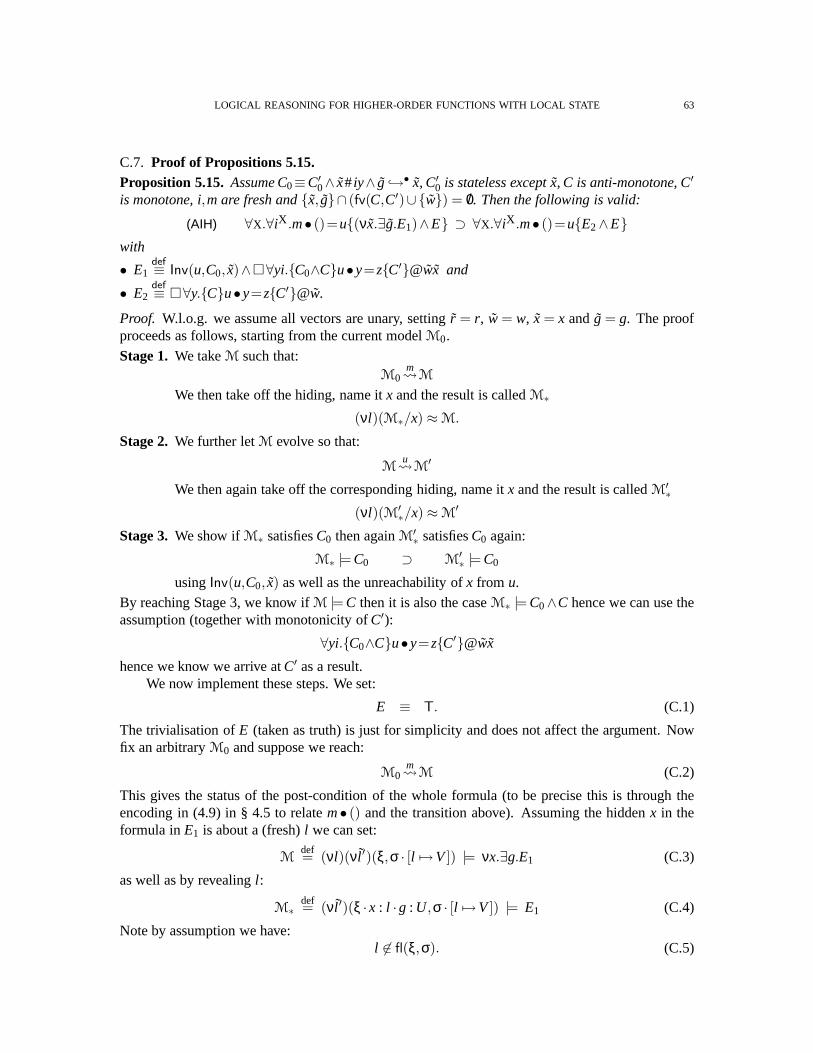
LOGICAL REASONING FOR HIGHER-ORDER FUNCTIONS WITH LOCAL STATE 63
C.7. Proof of Propositions 5.15.Proposition 5.15. Assume C0≡C′
0∧ x#iy∧ g →• x, C′0 is stateless exceptx, C is anti-monotone, C′
is monotone, i,m are fresh andx, g∩ (fv(C,C′)∪w) = /0. Then the following is valid:
(AIH) ∀X.∀iX .m• ()=u(νx.∃g.E1)∧E ⊃ ∀X.∀iX .m• ()=uE2∧E
with
• E1def≡ Inv(u,C0, x)∧∀yi.C0∧Cu•y=zC′@wx and
• E2def≡ ∀y.Cu•y=zC′@w.
Proof. W.l.o.g. we assume all vectors are unary, setting ˜r = r, w = w, x = x andg = g. The proofproceeds as follows, starting from the current modelM0.
Stage 1.We takeM such that:M0
m M
We then take off the hiding, name itx and the result is calledM∗
(νl)(M∗/x) ≈ M.
Stage 2.We further letM evolve so that:
Mu M
′
We then again take off the corresponding hiding, name itx and the result is calledM′∗
(νl)(M′∗/x) ≈ M
′
Stage 3.We show ifM∗ satisfiesC0 then againM′∗ satisfiesC0 again:
M∗ |= C0 ⊃ M′∗ |= C0
usingInv(u,C0, x) as well as the unreachability ofx from u.By reaching Stage 3, we know ifM |= C then it is also the caseM∗ |= C0∧C hence we can use theassumption (together with monotonicity ofC′):
∀yi.C0∧Cu•y=zC′@wx
hence we know we arrive atC′ as a result.We now implement these steps. We set:
E ≡ T. (C.1)
The trivialisation ofE (taken as truth) is just for simplicity and does not affect the argument. Nowfix an arbitraryM0 and suppose we reach:
M0m M (C.2)
This gives the status of the post-condition of the whole formula (to be precise this is through theencoding in (4.9) in § 4.5 to relatem• () and the transition above). Assuming the hiddenx in theformula inE1 is about a (fresh)l we can set:
Mdef= (νl)(νl ′)(ξ,σ · [l 7→V]) |= νx.∃g.E1 (C.3)
as well as by revealingl :
M∗def= (νl ′)(ξ ·x : l ·g : U,σ · [l 7→V]) |= E1 (C.4)
Note by assumption we have:l 6∈ fl(ξ,σ). (C.5)
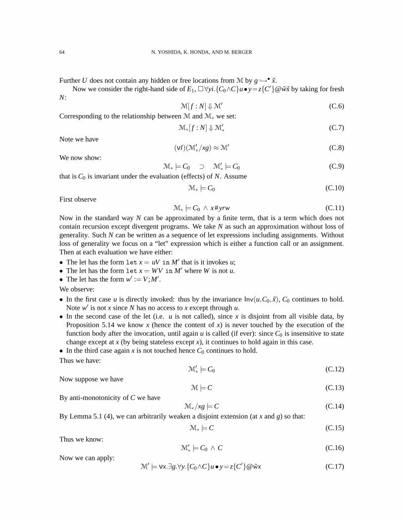
64 N. YOSHIDA, K. HONDA, AND M. BERGER
FurtherU does not contain any hidden or free locations fromM by g →• x.Now we consider the right-hand side ofE1,∀yi.C0∧Cu•y=zC′@wx by taking for fresh
N:M[ f : N] ⇓ M
′ (C.6)
Corresponding to the relationship betweenM andM∗ we set:
M∗[ f : N] ⇓ M′∗ (C.7)
Note we have(νl)(M′
∗/xg) ≈ M′ (C.8)
We now show:M∗ |= C0 ⊃ M
′∗ |= C0 (C.9)
that isC0 is invariant under the evaluation (effects) ofN. Assume
M∗ |= C0 (C.10)
First observeM∗ |= C0 ∧ x#yrw (C.11)
Now in the standard wayN can be approximated by a finite term, that is a term which does notcontain recursion except divergent programs. We takeN as such an approximation without loss ofgenerality. SuchN can be written as a sequence of let expressions including assignments. Withoutloss of generality we focus on a “let” expression which is either a function call or an assignment.Then at each evaluation we have either:
• The let has the formlet x = uV in M′ that is it invokesu;• The let has the formlet x = WV in M′ whereW is notu.• The let has the formw′ := V;M′.We observe:
• In the first caseu is directly invoked: thus by the invarianceInv(u,C0, x), C0 continues to hold.Notew′ is notx sinceN has no access tox except throughu.
• In the second case of the let (i.e.u is not called), sincex is disjoint from all visible data, byProposition 5.14 we knowx (hence the content ofx) is never touched by the execution of thefunction body after the invocation, until againu is called (if ever): sinceC0 is insensitive to statechange except atx (by being stateless exceptx), it continues to hold again in this case.
• In the third case againx is not touched henceC0 continues to hold.
Thus we have:M
′∗ |= C0 (C.12)
Now suppose we haveM |= C (C.13)
By anti-monotonicity ofC we haveM∗/xg |= C (C.14)
By Lemma 5.1 (4), we can arbitrarily weaken a disjoint extension (atx andg) so that:
M∗ |= C (C.15)
Thus we know:M
′∗ |= C0 ∧ C (C.16)
Now we can apply:M
′ |= νx.∃g.∀y.C0∧Cu•y=zC′@wx (C.17)

LOGICAL REASONING FOR HIGHER-ORDER FUNCTIONS WITH LOCAL STATE 65
by which we know:M
′∗[z : uy] ⇓ M
′′∗ |= C′ (C.18)
Accordingly letM
′[z : uy] ⇓ M′′ ≈ (νl)(M′′
∗/x) (C.19)
for which we know, by (C.18) and (C.19) together with monotonicity of C′:
M′′ |= C′ (C.20)
Hence we know:M |= Cu•y = zC′@w (C.21)
which is the required assertion. ⊓⊔
C.8. Proof of Proposition 5.16.Proposition 5.16. Let x 6∈ fv(C) and m, i,X be fresh. Then the following is valid:
∀X, iX .m• ()=uνx.([!x]C∧ x#uiX ) ⊃ m• ()=uC
Proof. For simplicity, set ˜x to be a singletonx. Assume
M[u : m()] ⇓ M′
By assumption we can setM
′ ≈ (νl)(νl ′)(ξ ·u : V,σ · l 7→W)
such that(νl ′)(ξ ·u : V ·x : l ,σ · l 7→W) |= [!x]C
wherel is not reachable from anywhere else in the model. By Lemma B.1we obtain(νl ′)(ξ ·u :V,σ) |= C, that isM′ |= C, as required. ⊓⊔
C.9. Proof of Proposition 5.17. AssumeC0 is stateless except ˜x and suppose:
M |= Inv( f ,C0, x) ∧ Tg• f = zT. (C.22)
Further assumeM M0 and
M0 |= C0∧ x#gr and M0[z : f g] ⇓ M′. (C.23)
By Inv( f ,C0, x) we know that onceC0 holds andf is invoked, it continues to hold. ByTg• f =zT, we know the applicationg f always terminates. Now this application invokesf zero or moretimes. First time it can only applyf to some ˜x-unreachable datum. Similarly for the second time,since the context cannot obtain ˜x-reachable datum (giveng itself is x-unreachable). By induction thesame holds up to the last invocation. In each invocation,C0 is invariant. Further, other computationsin f g never touch the content of ˜x, hence because ofC0 being stateless except ˜x, we knowC0 is againinvariant in such computations. Thus we conclude thatC0 still holds in the post-condition, and thatthe return value being ˜x-unreachable, i.e. ˜x#z, as required. ⊓⊔
APPENDIX D. DERIVATIONS FOR EXAMPLES IN SECTION 6
This appendix lists the derivations omitted in Section 6.

66 N. YOSHIDA, K. HONDA, AND M. BERGER
1. (n≥ 1⊃ IsEven′(!y,gh,n−1,xy)) ∧ n = 0 f :z z= Odd(n) ∧ !x = g∧ !y = h@/0(Const)
2. (n≥ 1⊃ IsEven′(!y,gh,n−1,xy)) ∧ n≥ 1not((!y)(n−1)) :z z= Odd(n) ∧ !x = g∧ !y = h@/0 (Simple, App)
3. n≥ 1⊃ IsEven′(!y,gh,n−1,xy)if n = 0 then f else not((!y)(n−1)) :m z= Odd(n) ∧ !x = g∧ !y = h@/0 (IfH)
4. T λn.if n = 0 then f else not((!y)(n−1)) :u ∀gh,n≥ 1.IsEven′(h,gh,n−1,xy)u•n=zz= Odd(n) ∧ !x = g∧ !y = h@/0@/0
(Abs, ∀, Conseq)
5. T Mx :u ∀gh,n≥ 1.(IsEven(h,gh,n−1,xy)⊃ IsOdd(u,gh,n,xy))@/0 (Conseq)
6. T x := Mx ∀gh,n≥ 1.(IsEven(h,gh,n−1,xy)⊃ IsOdd(!x,gh,n,xy)) ∧ !x = g@x(Assign)
7. T y := My ∀gh,n≥ 1.(IsOdd(g,gh,n−1,xy)⊃ IsEven(!y,gh,n,xy)) ∧ !y = h@y
8. T mutualParity∀gh.n≥ 1.((IsEven(h,gh,n−1,xy)∧ IsOdd(g,gh,n−1,xy))⊃
(IsEven(!y,gh,n,xy)∧ IsOdd(!x,gh,n,xy)∧!x= g∧!y = h) @xy (∧-Post)
9. T mutualParity∀n≥ 1gh.((IsEven(h,gh,n−1,xy)∧ IsOdd(g,gh,n−1,xy)∧!x= g∧!y= h) ⊃
(IsEven(!y,gh,n,xy)∧ IsOdd(!x,gh,n,xy)∧!x= g∧!y = h)@xy (Conseq)
10. T mutualParity∀n≥ 1gh.((IsEven(!y,gh,n−1,xy)∧ IsOdd(!x,gh,n−1,xy)∧!x= g∧!y = h) ⊃
(IsEven(!y,gh,n,xy)∧ IsOdd(!x,gh,n,xy)∧!x= g∧!y = h)@xy (Conseq)
11. T mutualParity∀n≥ 1.(∃gh.(IsEven(!x,gh,n−1,xy)∧ IsOdd(!y,gh,n−1,xy)∧!x= g∧!y = h) ⊃∃gh.(IsEven(!y,gh,n,xy)∧ IsOdd(!x,gh,n,xy)∧!x= g∧!y = h)@xy (Conseq)
12. T mutualParity∃gh.IsOddEven(gh, !x!y,xy,n)@xy
Figure 7:mutualParity derivations
D.1. Derivation for mutualParity. Let us define:
Mxdef= λn.if y = 0 then f else not((!y)(n−1))
Mydef= λn.if y = 0 then t else not((!x)(n−1))
We also use:
IsOdd′(u,gh,n,xy)def
≡ IsOdd(u,gh,n,xy)∧ !x = g∧ !y = h
IsEven′(u,gh,n,xy)def
≡ IsEven(u,gh,n,xy)∧ !x = g∧ !y = h
Figure 7 lists the derivation forMutualParity. In Line 4, h in the evaluation formula can bereplaced by !y and vice versa because of !y = h and the universal quantification ofh.
∀h.(!y = h∧Ch•n = zC′) ≡ ∀h.(!y = h∧C(!y)•n = zC′)

LOGICAL REASONING FOR HIGHER-ORDER FUNCTIONS WITH LOCAL STATE 67
In Line 5, we use the following axiom for the evaluation formula from [25]:
C∧A e1•e2 = zC′ ≡ A ⊃ Ce1 •e2 = zC′
whereA is stateless and we setA= IsEven(h,gh,n−1,xy). Line 9 is derived as Line 4 by replacingh and g by !y and !x, respectively. Line 11 is the standard logical implication(∀x.(C1 ⊃ C2) ⊃(∃x.C1 ⊃ ∃x.C2)).
D.2. Derivation for Meyer-Sieber. For the derivation of (6.6) we use:
Edef≡ ∀ f .(T f • ()T@/0 ⊃ Cg• fC′)
We use the following[LetRef] which is derived by[Ref] whereC′ is replaced by[!x]C′.
[LetRef]C M :m C0 [!x]C0∧!x = m∧x#e N :u C
′ x /∈ fpn(e)C let x = ref(M) in N :u νx.C′
with C′ think w.r.t. m. The derivation follows. BelowM1,2 is the body of the first/second lets,respectively.
1.Even(!x)∧ [!x]C′ if even(!x) then () else Ω() [!x]C′@/0 (If)
2.[!x]C g f [!x]C′ (cf. § 6.7)
3.Even(!x)∧ [!x]C g f Even(!x)∧ [!x]C′ (2, Inv)
4.E∧ [!x]C∧Even(!x)∧x#gilet f = ... in (g f ; ...)[!x]C′ ∧x#i (3, Seq, Let)
5.E∧C MeyerSieber νx.([!x]C′ ∧x#i) (4, LetRef)
6.E∧C MeyerSieber C′ (9, Prop. 5.16)
D.3. Derivation for Object. We need the following generalisation. The procedureu in (AIH) is offunction typeα ⇒ β: when values of other types such asα×β or α+ β are returned, we can makeuse of a generalisation. For simplicity we restrict our attention to the case when types do not containrecursive or reference types.
Inv(uα×β,C0, x)def≡ ∧i=1,2Inv(πi(u),C0, x)
Inv(uα+β,C0, x)def≡ ∧i=1,2∀yi .(u = inji(yi) ⊃ Inv(yi ,C0, x))
Inv(uα,C0, x)def
≡ T (α ∈ Unit,Nat,Bool)
Using this extension, we can generalise(AIH) so that the cancelling ofC0 is possible for all com-ponents ofu. For example, ifu is a pair of functions, those two functions need to satisfy the samecondition as in(AIH). This is what we shall use forcellGen. We call the resulting generalisedaxiom (AIHc).
Let cell be the internalλ-abstraction ofcellGen. First, it is easy to obtain:
T cell :o I0 ∧ G1 ∧ G2 ∧ E′ (D.1)
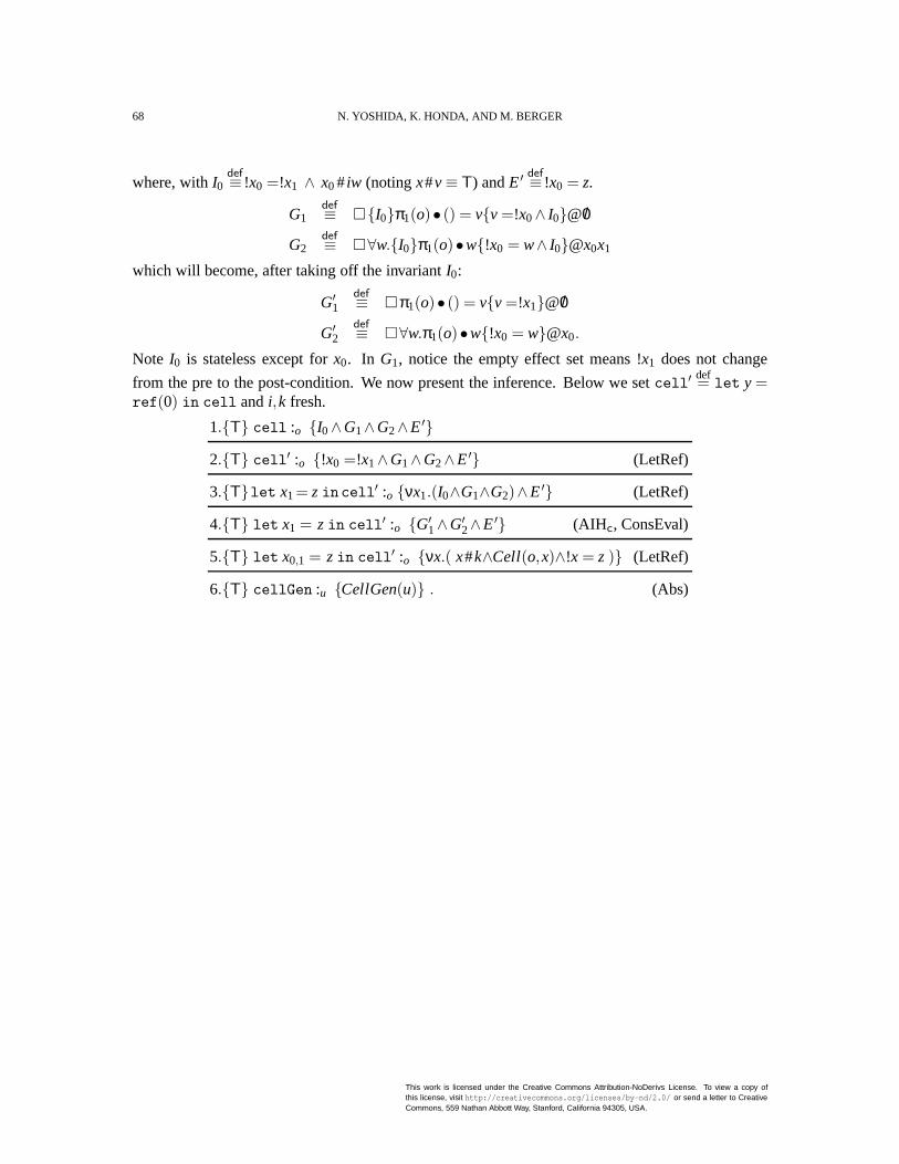
68 N. YOSHIDA, K. HONDA, AND M. BERGER
where, withI0def
≡ !x0 =!x1 ∧ x0 #iw (notingx#v≡ T) andE′ def
≡ !x0 = z.
G1def
≡ I0π1(o)• () = vv =!x0∧ I0@/0
G2def≡ ∀w.I0π1(o)•w!x0 = w∧ I0@x0x1
which will become, after taking off the invariantI0:
G′1
def≡ π1(o)• () = vv =!x1@/0
G′2
def≡ ∀w.π1(o)•w!x0 = w@x0.
Note I0 is stateless except forx0. In G1, notice the empty effect set means !x1 does not change
from the pre to the post-condition. We now present the inference. Below we setcell′def= let y =
ref(0) in cell andi,k fresh.
1.T cell :o I0∧G1∧G2∧E′
2.T cell′ :o !x0 =!x1∧G1∧G2∧E′ (LetRef)
3.Tlet x1= zincell′ :o νx1.(I0∧G1∧G2)∧E′ (LetRef)
4.T let x1 = zin cell′ :o G′1∧G′
2∧E′ (AIH c, ConsEval)
5.T let x0,1 = zin cell′ :o νx.( x#k∧Cell(o,x)∧!x = z ) (LetRef)
6.T cellGen :u CellGen(u) . (Abs)
This work is licensed under the Creative Commons Attribution-NoDerivs License. To view a copy ofthis license, visit http://creativecommons.org/licenses/by-nd/2.0/ or send a letter to CreativeCommons, 559 Nathan Abbott Way, Stanford, California 94305, USA.