1

Logarithmic functions of Y and/or X

Last class, we saw that we could approximate a model in which X has a

non-linear effect on Y by using a polynomial population model:

𝑌𝑖 = 𝛽0 + 𝛽1𝑋𝑖 + 𝛽2𝑋𝑖2 + 𝛽3𝑋𝑖

3 + ⋯ + 𝛽𝑟𝑋𝑖𝑟 + 𝑢𝑖

Other regressors may be added as usual

This is a polynomial of degree r

Often a quadratic or cubic term is enough

r can be determined by a series of t or F tests

The validity of this approximation is based on a Taylor series

expansion

2

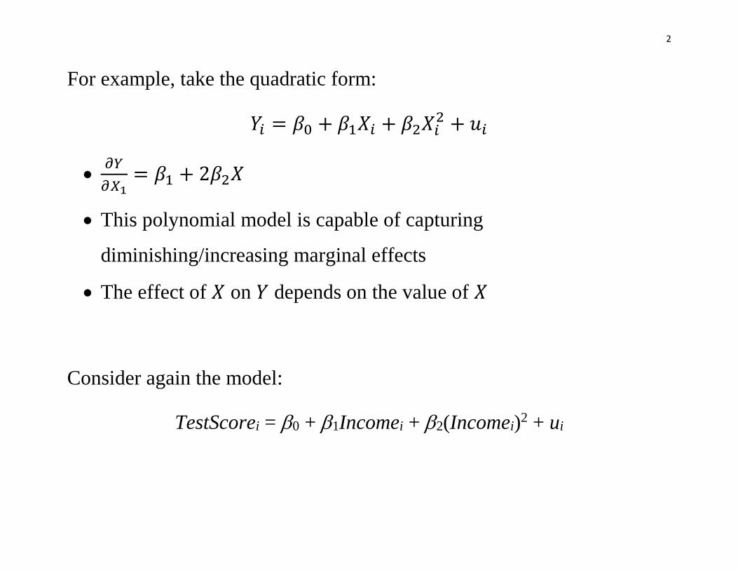
For example, take the quadratic form:

𝑌𝑖 = 𝛽0 + 𝛽1𝑋𝑖 + 𝛽2𝑋𝑖2 + 𝑢𝑖

𝜕𝑌

𝜕𝑋1= 𝛽1 + 2𝛽2𝑋

This polynomial model is capable of capturing

diminishing/increasing marginal effects

The effect of 𝑋 on 𝑌 depends on the value of 𝑋

Consider again the model:

TestScorei = 0 + 1Incomei + 2(Incomei)2 + ui

3

OLS estimates this model as:

𝑇𝑒𝑠𝑡𝑆𝑐𝑜𝑟𝑒̂𝑖 = 607.3 + 3.85𝐼𝑛𝑐𝑜𝑚𝑒𝑖 − 0.0423𝐼𝑛𝑐𝑜𝑚𝑒𝑖

2

(2.9) (0.27) (0.0048)

4

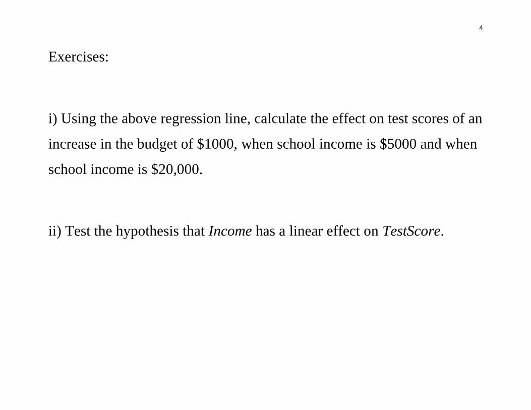
Exercises:

i) Using the above regression line, calculate the effect on test scores of an

increase in the budget of $1000, when school income is $5000 and when

school income is $20,000.

ii) Test the hypothesis that Income has a linear effect on TestScore.

5

Another way (besides using polynomials) to express a non-linear

relationship is in percentages. For example:

Wage gap across professions/time

Elasticity of demand – a 1% increase in P leads to a Q% decrease in

quantity demanded

Test scores and district income

The effect of age or yrseduc on earnings.

What kind of model should we estimate so that (for example) a change in

X causes a percentage change in Y?

6

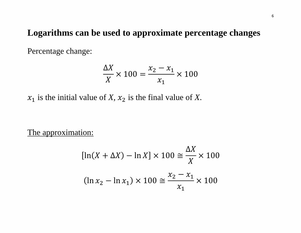
Logarithms can be used to approximate percentage changes

Percentage change:

∆𝑋

𝑋× 100 =

𝑥2 − 𝑥1

𝑥1× 100

𝑥1 is the initial value of X, 𝑥2 is the final value of X.

The approximation:

[ln(𝑋 + ∆𝑋) − ln 𝑋] × 100 ≅∆𝑋

𝑋× 100

(ln 𝑥2 − ln 𝑥1) × 100 ≅𝑥2 − 𝑥1

𝑥1× 100

7

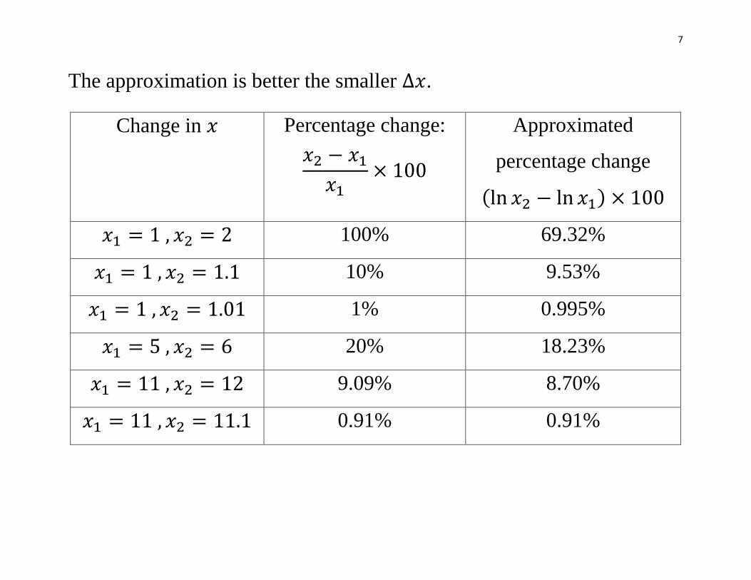
The approximation is better the smaller ∆𝑥.

Change in 𝑥 Percentage change:

𝑥2 − 𝑥1

𝑥1× 100

Approximated

percentage change

(ln 𝑥2 − ln 𝑥1) × 100

𝑥1 = 1 , 𝑥2 = 2 100% 69.32%

𝑥1 = 1 , 𝑥2 = 1.1 10% 9.53%

𝑥1 = 1 , 𝑥2 = 1.01 1% 0.995%

𝑥1 = 5 , 𝑥2 = 6 20% 18.23%

𝑥1 = 11 , 𝑥2 = 12 9.09% 8.70%

𝑥1 = 11 , 𝑥2 = 11.1 0.91% 0.91%

8

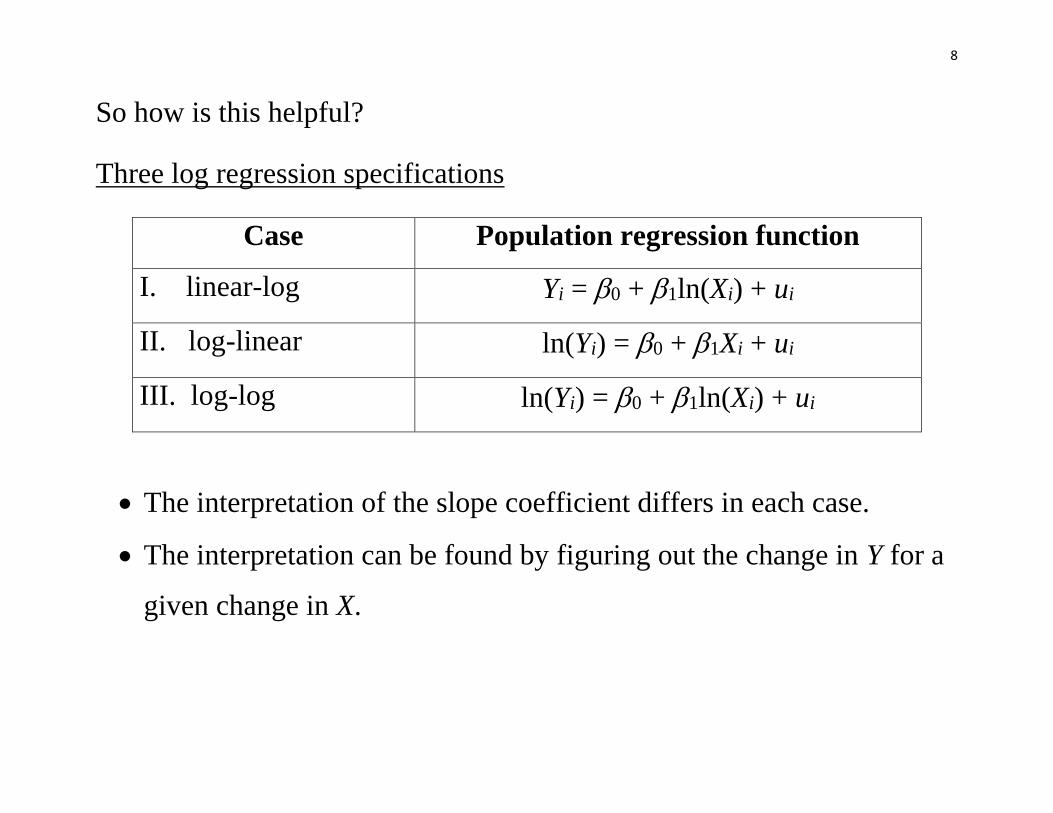
So how is this helpful?

Three log regression specifications

Case Population regression function

I. linear-log Yi = 0 + 1ln(Xi) + ui

II. log-linear ln(Yi) = 0 + 1Xi + ui

III. log-log ln(Yi) = 0 + 1ln(Xi) + ui

The interpretation of the slope coefficient differs in each case.

The interpretation can be found by figuring out the change in Y for a

given change in X.

9

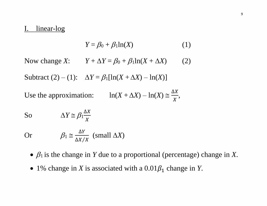
I. linear-log

Y = 0 + 1ln(X) (1)

Now change X: Y + Y = 0 + 1ln(X + X) (2)

Subtract (2) – (1): Y = 1[ln(X + X) – ln(X)]

Use the approximation: ln(X + X) – ln(X) ∆𝑋

𝑋,

So Y 1∆𝑋

𝑋

Or 1 ∆𝑌

∆𝑋 𝑋⁄ (small X)

1 is the change in Y due to a proportional (percentage) change in X.

1% change in X is associated with a 0.01𝛽1 change in Y.

10

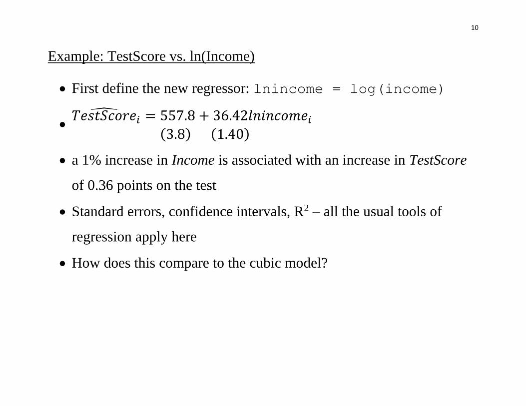
Example: TestScore vs. ln(Income)

First define the new regressor: lnincome = log(income)

𝑇𝑒𝑠𝑡𝑆𝑐𝑜𝑟𝑒̂

𝑖 = 557.8 + 36.42𝑙𝑛𝑖𝑛𝑐𝑜𝑚𝑒𝑖

(3.8) (1.40)

a 1% increase in Income is associated with an increase in TestScore

of 0.36 points on the test

Standard errors, confidence intervals, R2 – all the usual tools of

regression apply here

How does this compare to the cubic model?

11

12

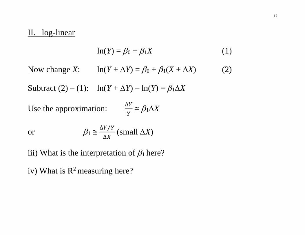
II. log-linear

ln(Y) = 0 + 1X (1)

Now change X: ln(Y + Y) = 0 + 1(X + X) (2)

Subtract (2) – (1): ln(Y + Y) – ln(Y) = 1X

Use the approximation: ∆𝑌

𝑌 1X

or 1 ∆𝑌 𝑌⁄

∆𝑋 (small X)

iii) What is the interpretation of 1 here?

iv) What is R2 measuring here?

13

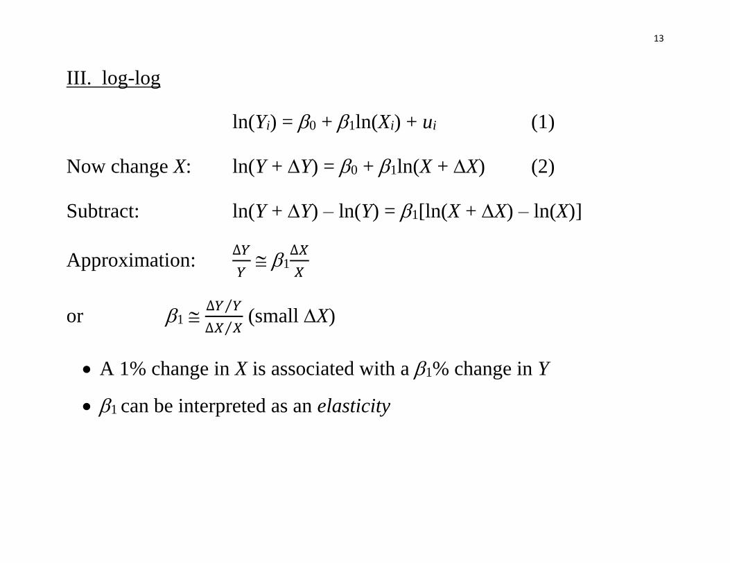
III. log-log

ln(Yi) = 0 + 1ln(Xi) + ui (1)

Now change X: ln(Y + Y) = 0 + 1ln(X + X) (2)

Subtract: ln(Y + Y) – ln(Y) = 1[ln(X + X) – ln(X)]

Approximation: ∆𝑌

𝑌 1

∆𝑋

𝑋

or 1 ∆𝑌 𝑌⁄

∆𝑋 𝑋⁄ (small X)

A 1% change in X is associated with a 1% change in Y

1 can be interpreted as an elasticity

14

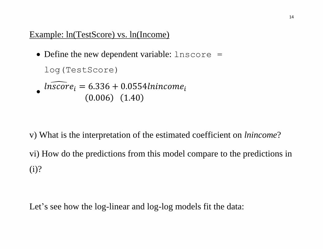
Example: ln(TestScore) vs. ln(Income)

Define the new dependent variable: lnscore =

log(TestScore)

𝑙𝑛𝑠𝑐𝑜𝑟𝑒̂

𝑖 = 6.336 + 0.0554𝑙𝑛𝑖𝑛𝑐𝑜𝑚𝑒𝑖

(0.006) (1.40)

v) What is the interpretation of the estimated coefficient on lnincome?

vi) How do the predictions from this model compare to the predictions in

(i)?

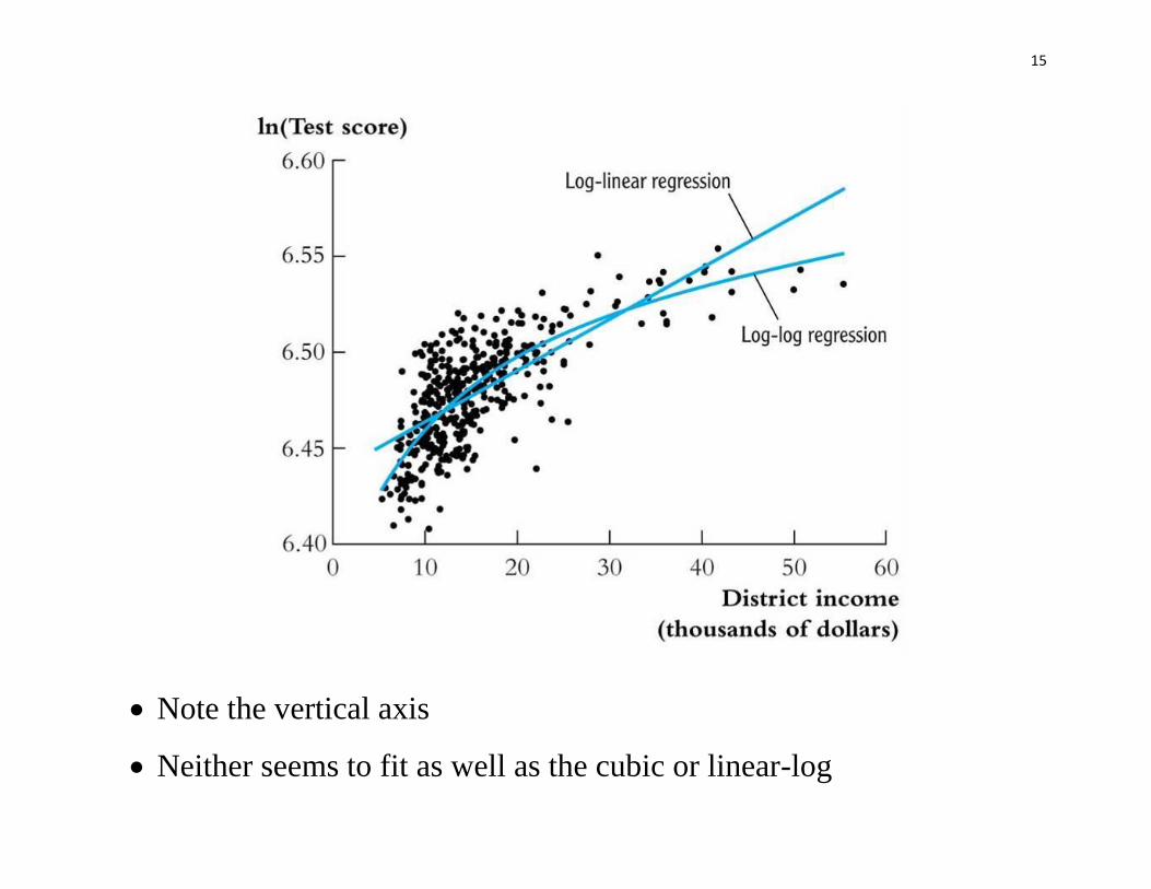
Let’s see how the log-linear and log-log models fit the data:

15

Note the vertical axis

Neither seems to fit as well as the cubic or linear-log

16

Summary: Logarithmic transformations

Three cases, differing in whether Y and/or X is transformed by taking

logs

Hypothesis tests and confidence intervals are now implemented and

interpreted “as usual”

The interpretation of 1 differs from case to case

Choice of specification should be guided by judgment (which

interpretation makes the most sense in your application?), tests, and

plotting predicted values

17

Extensions: Non-linear effects

We can still use OLS as long as the model we are trying to estimate is

linear in the parameters (𝛽𝑠). That is,

𝑌 = 𝛽0 + 𝛽1∎ + 𝛽2∎ + ⋯

is still linear in the parameters, even though the stuff in the boxes may

be non-linear transformations of the X variables.

OLS is surprisingly capable of capturing non-linear effects. Consider the

Cobb-Douglas production function:

𝑌 = 𝐴𝐾𝛼𝐿𝛽

18

vii) What parameters would you be trying to estimate?

viii) Is the model linear in these parameters?

ix) If not, can you make a transformation?

19

cobbdata=read.csv("http://home.cc.umanitoba.ca/~godwinrt/7010/cobb.

csv")

attach(cobbdata)

summary(lm(log(y) ~ log(k) + log(l)))

Call:

lm(formula = log(y) ~ log(k) + log(l))

Coefficients:

Estimate Std. Error t value Pr(>|t|)

(Intercept) 1.8444 0.2336 7.896 7.33e-08 ***

log(k) 0.2454 0.1069 2.297 0.0315 *

log(l) 0.8052 0.1263 6.373 2.06e-06 ***

---

Signif. codes: 0 ‘***’ 0.001 ‘**’ 0.01 ‘*’ 0.05 ‘.’ 0.1 ‘ ’ 1

Residual standard error: 0.2357 on 22 degrees of freedom

Multiple R-squared: 0.9731, Adjusted R-squared: 0.9706

F-statistic: 397.5 on 2 and 22 DF, p-value: < 2.2e-16

20

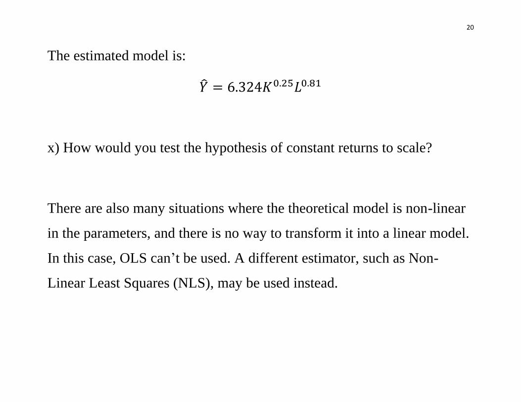
The estimated model is:

�̂� = 6.324𝐾0.25𝐿0.81

x) How would you test the hypothesis of constant returns to scale?

There are also many situations where the theoretical model is non-linear

in the parameters, and there is no way to transform it into a linear model.

In this case, OLS can’t be used. A different estimator, such as Non-

Linear Least Squares (NLS), may be used instead.