Locally adaptive density estimation on Riemannian manifolds - Idescat

Statistics & Operations Research Transactions

SORT 37 (2) July-December 2013, 111-130

Statistics &Operations Research

Transactionsc© Institut d’Estadıstica de Catalunya

[email protected]: 1696-2281eISSN: 2013-8830www.idescat.cat/sort/

Locally adaptive density estimation on

Riemannian manifolds

Guillermo Henry1,2, Andres Munoz1 and Daniela Rodriguez1,2

Abstract

In this paper, we consider kernel type estimator with variable bandwidth when the random vari-

ables belong in a Riemannian manifolds. We study asymptotic properties such as the consistency

and the asymptotic distribution. A simulation study is also considered to evaluate the performance

of the proposal. Finally, to illustrate the potential applications of the proposed estimator, we anal-

yse two real examples where two different manifolds are considered.

MSC: 62G07, 62G20

Keywords: Asymptotic results, density estimation, nonparametric, Riemannian manifolds.

1. Introduction

Let X1, . . . ,Xn be independent and identically distributed random variables taking values

in Rd and having density function f . A class of estimators of f which has been widely

studied since the work of Rosenblatt (1956) and Parzen (1962) has the form

fn(x) =1

nhd

n

∑j=1

K

(x−X j

h

),

where K(u) is a bounded density on Rd and h is a sequence of positive number such that

h → 0 and nhd → ∞ as n → ∞.

If we apply this estimator to data coming from long tailed distributions, with a small

enough h to be appropriate for the central part of the distribution, a spurious noise ap-

1 Facultad de Ciencias Exactas y Naturales, Universidad de Buenos Aires.2 CONICET, Argentina.

[email protected], [email protected] and [email protected]

Received: April 2012

Accepted: January 2013

112 Locally adaptive density estimation on Riemannian manifolds

pears in the tails. With a large value of h for correctly handling the tails, we can

not see the details occurring in the main part of the distribution. To overcome these

defects, adaptive kernel estimators were introduced. For instance, a conceptually similar

estimator of f (x) was studied by Wagner (1975) who defined a general neighbour

density estimator by

fn(x) =1

nHdn (x)

n

∑j=1

K

(x−X j

Hn(x)

),

where Hn(x) is the distance between x and the k-nearest neighbour of x among X1, . . . ,Xn,

and k = kn is a sequence of non–random integers such that limn→∞ kn = ∞. Through this

adaptive bandwidth , the estimation in the point x has the guarantee that to be calculated

using at least k points of the sample.

However, in many applications, the variables X take values on different spaces than

Rd . Usually these spaces have a more complicated geometry than the Euclidean space

and this has to be taken into account in the analysis of the data. For example, if we study

the distribution of the stars with luminosity in a given range it is natural to think that the

variables belong to a spherical cylinder (S2 ×R) instead of R4. If we consider a region

of the planet M, then the direction and the velocity of the wind in this region are points

in the tangent bundle of M, that is a manifold of dimension 4. Other examples could be

found in image analysis, mechanics, geology and other fields. They include distributions

on spheres, Lie groups, among others, see for example Joshi et al. (2007), Goh and Vidal

(2008). For this reason, it is interesting to study an estimation procedure of the density

function that takes into account a more complex structure of the variables.

Nonparametric kernel methods for estimating densities of spherical data have been

studied by Hall et al. (1987) and Bai et al. (1988). Pelletier (2005) proposed a family

of nonparametric estimators for the density function based on kernel weighting when

the variables are random objects valued in a closed Riemannian manifold. Pelletier’s

estimators are consistent with the kernel density estimators in the Euclidean case

considered by Rosenblatt (1956) and Parzen (1962).

As we comment above, the importance of local adaptive bandwidth is well known in

nonparametric statistics and this is even more true with data taking values in complex

spaces. In this paper, we propose a kernel density estimator on a Riemannian manifold

with a variable bandwidth defined by k-nearest neighbours.

This paper is organized as follows. Section 2 contains a brief summary of the

necessary concepts of Riemannian geometry. In Section 2.1, we introduce the estimator.

Uniform consistency of the estimator is derived in Section 3.1, while in Section 3.2

the asymptotic distribution is obtained under regular assumptions. Section 4 contains

a Monte Carlo study designed to evaluate the proposed estimator. Finally, Section 5

presents two example using real data. Proofs are given in the Appendix.

Guillermo Henry, Andres Munoz and Daniela Rodriguez 113

2. Preliminaries and the estimator

Let (M,g) be a d-dimensional Riemannian manifold without boundary. We denote by

dg the distance induced by the metric g. With Bs(p) we denote a normal ball with radius

s centred at p. The injectivity radius of (M,g) is given by in jgM = infp∈M

sup{s ∈ R> 0 :

Bs(p) is a normal ball}. It is easy to see that a compact Riemannian manifold has strictly

positive injectivity radius. For example, it is not difficult to see that the d-dimensional

sphere Sd endowed with the metric induced by the canonical metric g0 of Rd+1 has

injectivity radius equal to π. If N is a proper submanifold of the same dimension than

(M,g), then in jg|N N = 0. The Euclidean space or the hyperbolic space have infinite

injectivity radius. Moreover, a complete and simply connected Riemannian manifold

with non-positive sectional curvature has also this property.

Throughout this paper, we will assume that (M,g) is a complete Riemannian mani-

fold, i.e. (M,dg) is a complete metric space. Also we will consider that in jgM is strictly

positive. This restriction will be clear in the Section 2.1 when we define the estima-

tor. For standard result on differential and Riemannian geometry we refer to the reader

to Boothby (1975), Besse (1978), Do Carmo (1988) and Gallot, Hulin and Lafontaine

(2004).

Let p ∈ M, we denote with 0p and TpM the null tangent vector and the tangent space

of M at p. Let Bs(p) be a normal ball centred at p. Then Bs(0p) = exp−1p (Bs(p)) is

an open neighbourhood of 0p in TpM and so it has a natural structure of differential

manifold. We are going to consider the Riemannian metrics g ′ and g ′ ′ in Bs(0p), where

g ′ = exp∗p(g) is the pullback of g by the exponential map and g ′ ′ is the canonical metric

induced by gp in Bs(0p). Let w∈Bs(0p), and (U ,ψ) be a chart of Bs(0p) such that w∈ U .

We note by {∂/∂ ψ1|w, . . . ,∂/∂ ψd |w} the tangent vectors induced by (U ,ψ). Consider

the matricial function with entries (i, j) are given by g ′ ((∂/∂ ψi|w),(∂/∂ ψ j|w

)).

The volumes of the parallelepiped spanned by {(∂/∂ ψ1|w

), . . . ,

(∂/∂ ψd |w

)} with

respect to the metrics g ′ and g ′ ′ are given by |detg ′ ((∂/∂ ψi|w),(∂/∂ ψ j|w

))|1/2

and |detg ′ ′ ((∂/∂ ψi|w),(∂/∂ ψ j|w

))|1/2 respectively. The quotient between these two

volumes is independent of the selected chart. So, given q ∈ Bs(p), if w = exp−1p (q) ∈

Bs(0p) we can define the volume density function, θp(q), on (M,g) as

θp(q) =|detg ′ ((∂/∂ ψi|w

),(∂/∂ ψ j|w

))|1/2

|detg ′ ′ ((∂/∂ ψi|w),(∂/∂ ψ j|w

))|1/2

for any chart (U ,ψ) of Bs(0p) that contains w = exp−1p (q). For instance, if we consider

a normal coordinate system (U,ψ) induced by an orthonormal basis {v1, . . . ,vd} of TpM

then θp(q) is the function of the volume element dνg in the local expression with respect

to chart (U,ψ) evaluated at q, i.e.

θp(q) =

∣∣∣∣detgq

(∂

∂ψi

∣∣∣q,

∂

∂ψ j

∣∣∣q

)∣∣∣∣12

,


where ∂∂ψi

|q = Dαi(0)expp(αi(0)) with αi(t) = exp−1p (q)+ tvi for q ∈ U . Note that the

volume density function θp(q) is not defined for all the pairs p and q in M, but it is if

dg(p,q)< in jgM.

We finish the section showing some examples of the density function:

i) In the case of (Rd,g0) the density function is θp(q) = 1 for all (p,q) ∈ Rd ×Rd .

ii) In the 2-dimensional sphere of radius R, the volume density is

θp1(p2) = R

|sin(dg(p1, p2)/R)|dg(p1, p2)

if p2 6= p1,−p1 and θp1(p1) = 1.

where dg induced is given by

dg(p1, p2) = Rarccos

(〈p1, p2〉R2

).

iii) In the case of the cylinder of radius 1 C1 endowed with the metric induced by the

canonical metric of R3, θp1(p2) = 1 for all (p1, p2) ∈C1 ×C1, and the distance

induced is given by dg(p1, p2) = d2((r1,s1),(r2,s2)) if d2((r1,s1),(r2,s2)) < π,

where d2 is the Euclidean distance of R2 and pi = (cos(ri),sin(ri),si) for i = 1,2.

See also Besse (1978) and Pennec (2006) for a discussion on the volume density

function.

2.1. The estimator

Consider a probability distribution with a density f on a d-dimensional Riemannian

manifold (M,g). Let X1, · · · ,Xn be i.i.d random object taking values on M with density

f . A natural extension of the estimator proposed by Wagner (1975) in the context of a

Riemannian manifold is to consider the following estimator

fn(p) =1

nHdn (p)

n

∑j=1

1

θX j(p)

K

(dg(p,X j)

Hn(p)

),

where K : R→ R is a non-negative function with compact support, θp(q) denotes the

volume density function on (M,g) and Hn(p) is the distance dg between p and the

k-nearest neighbour of p among X1, . . . ,Xn, and k = kn is a sequence of non-random

integers such that limn→∞ kn = ∞.

As we mention above, the volume density function is not defined for all p and

q. Therefore, in order to guarantee the well definition of the estimator we consider a

modification of the proposed estimator. Using the fact that the kernel K has compact


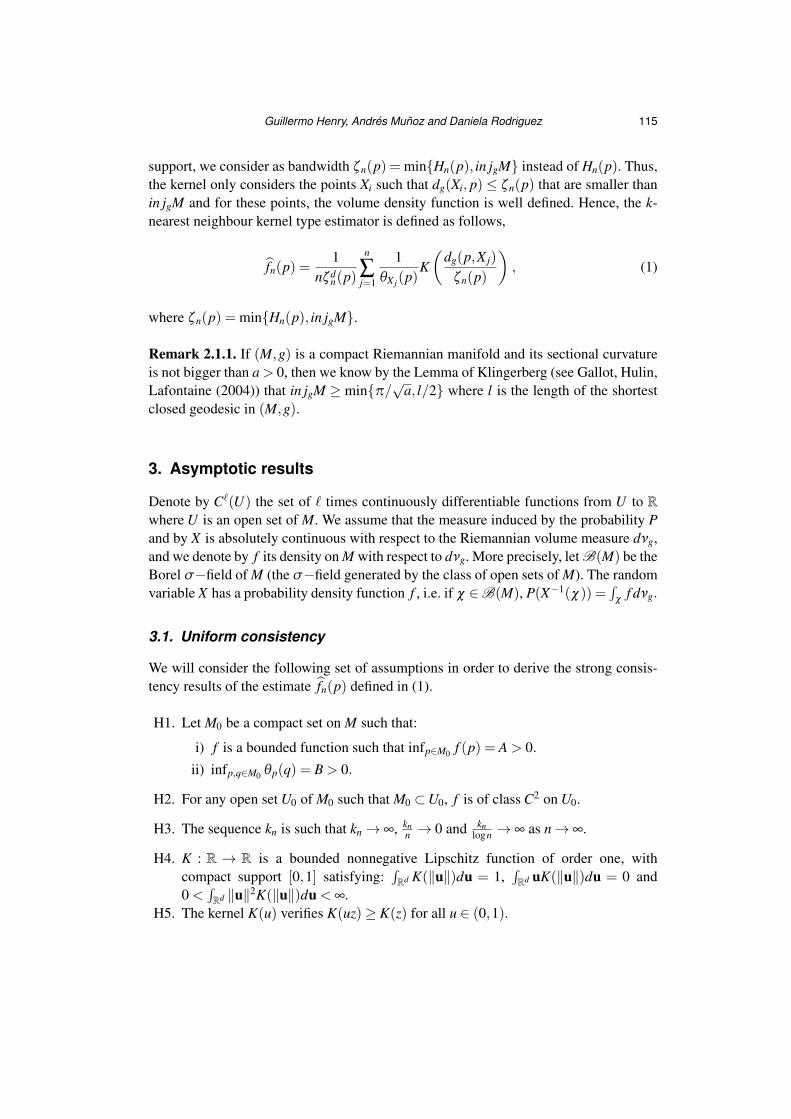
support, we consider as bandwidth ζn(p) = min{Hn(p), in jgM} instead of Hn(p). Thus,

the kernel only considers the points Xi such that dg(Xi, p)≤ ζn(p) that are smaller than

in jgM and for these points, the volume density function is well defined. Hence, the k-

nearest neighbour kernel type estimator is defined as follows,

fn(p) =1

nζdn(p)

n

∑j=1

1

θX j(p)

K

(dg(p,X j)

ζn(p)

), (1)

where ζn(p) = min{Hn(p), in jgM}.

Remark 2.1.1. If (M,g) is a compact Riemannian manifold and its sectional curvature

is not bigger than a > 0, then we know by the Lemma of Klingerberg (see Gallot, Hulin,

Lafontaine (2004)) that in jgM ≥ min{π/√a, l/2} where l is the length of the shortest

closed geodesic in (M,g).

3. Asymptotic results

Denote by Cℓ(U) the set of ℓ times continuously differentiable functions from U to R

where U is an open set of M. We assume that the measure induced by the probability P

and by X is absolutely continuous with respect to the Riemannian volume measure dνg,

and we denote by f its density on M with respect to dνg. More precisely, let B(M) be the

Borel σ−field of M (the σ−field generated by the class of open sets of M). The random

variable X has a probability density function f , i.e. if χ ∈B(M), P(X−1(χ)) =∫χ f dνg.

3.1. Uniform consistency

We will consider the following set of assumptions in order to derive the strong consis-

tency results of the estimate fn(p) defined in (1).

H1. Let M0 be a compact set on M such that:

i) f is a bounded function such that infp∈M0f (p) = A > 0.

ii) infp,q∈M0θp(q) = B > 0.

H2. For any open set U0 of M0 such that M0 ⊂U0, f is of class C2 on U0.

H3. The sequence kn is such that kn → ∞, kn

n→ 0 and kn

logn→ ∞ as n → ∞.

H4. K : R → R is a bounded nonnegative Lipschitz function of order one, with

compact support [0,1] satisfying:∫Rd K(‖u‖)du = 1,

∫Rd uK(‖u‖)du = 0 and

0 <∫Rd ‖u‖2K(‖u‖)du < ∞.

H5. The kernel K(u) verifies K(uz)≥ K(z) for all u ∈ (0,1).


Remark 3.1.1. The fact that θp(p) = 1 for all p ∈ M guarantees that H1 ii) holds. The

assumption H3 is usual when dealing with nearest neighbor and the assumption H4 is

standard when dealing with kernel estimators.

Theorem 3.1.2. Assume that H1 to H5 holds, then we have that

supp∈M0

| fn(p)− f (p)| a.s.−→ 0.

3.2. Asymptotic normality

To derive the asymptotic distribution of the regression parameter estimates we will

need two additional assumptions. We will denote with Vr the Euclidean ball of radius r

centered at the origin and with λ(Vr) its Lebesgue measure.

H5. f (p) > 0, f ∈ C2(V ) with V ⊂ M an open neighborhood of M and the second

derivative of f is bounded.

H6. The sequence kn is such that kn →∞, kn/n→ 0 as n→∞ and there exists 0≤β <∞

such that√

knn−4/(d+4) → β as n → ∞.

H7. The kernel verifies

i)∫

K1(‖u‖)‖u‖2du < ∞ as s → ∞ where K1(u) = K′(‖u‖)‖u‖.

ii) ‖u‖d+1K2(u)→ 0 as ‖u‖→ ∞ where K2(u) = K′′(‖u‖)‖u‖2 −K1(u)

Remark 3.2.1. Note that div(K(‖u‖)u) =K′(‖u‖)‖u‖+d K(‖u‖), then using the diver-

gence Theorem, we get that∫

K′(‖u‖)‖u‖du =∫‖u‖=1 K(‖u‖)u u

‖u‖du−d∫

K(‖u‖)du.

Thus, the fact that K has compact support in [0,1] implies that∫

K1(u)du =−d.

On the other hand, note that ∇(K(‖u‖)‖u‖2) = K1(‖u‖)u+ 2K(‖u‖)u and by H4

we get that∫

K1(‖u‖)udu = 0.

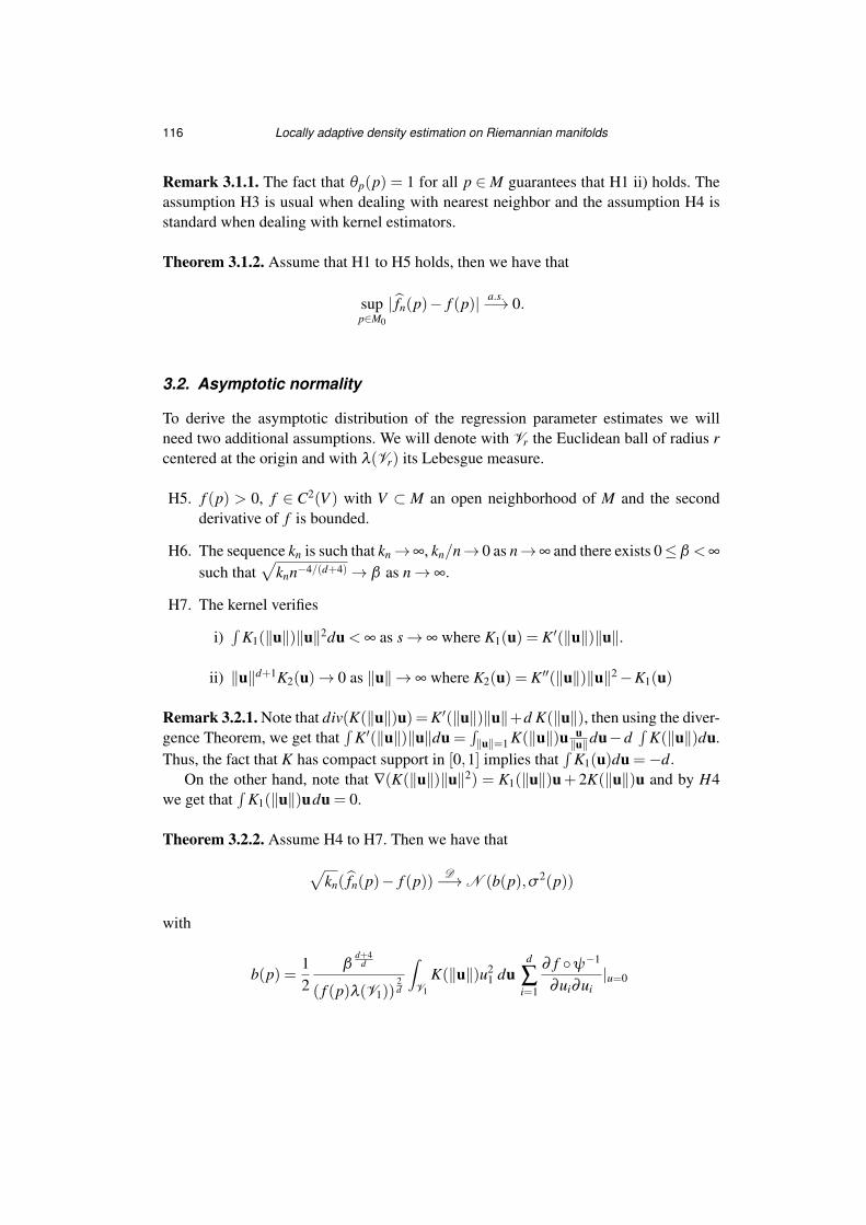
Theorem 3.2.2. Assume H4 to H7. Then we have that

√kn( fn(p)− f (p))

D−→ N (b(p),σ2(p))

with

b(p) =1

2

βd+4

d

( f (p)λ(V1))2d

∫

V1

K(‖u‖)u21 du

d

∑i=1

∂ f ◦ψ−1

∂ui∂ui

|u=0


and

σ2(p) = λ(V1) f 2(p)∫

V1

K2(‖u‖)du

where u = (u1, . . . ,ud) and (Bh(p),ψ) is any normal coordinate system.

In order to derive the asymptotic distribution of fn(p), we will study the asymptotic

behaviour of hdn/ζ

dn(p) where hd

n = kn/(n f (p)λ(V1)). Note that if we consider fn(p) =

kn/(nζdn(p)λ(V1)), fn(p) is a consistent estimator of f (p) (see the proof of Theorem

3.1.2). The next Theorem states that this estimator is also asymptotically normally

distributed as in the Euclidean case.

Theorem 3.2.3. Assume H4 to H6, and let hdn = kn/(n f (p)λ(V1)). Then we have that

√kn

(hd

n

ζdn(p)

−1

)D−→ N(b1(p),1)

with

b1(p) =

(β

d+42

f (p)µ(V1)

) 2d{

τ

6d +12+

∫V1

u21 du L1(p)

f (p)µ(V1)

}

where u = (u1, . . . ,ud), τ is the scalar curvature of (M,g), i.e. the trace of the Ricci

tensor,

L1(p) =d

∑i=1

(∂ 2 f ◦ψ−1

∂uiui

∣∣∣u=0

+∂ f ◦ψ−1

∂ui

∣∣∣u=0

∂θp ◦ψ−1

∂ui

∣∣∣u=0

)

and (Bh(p),ψ) is any normal coordinate system.

4. Simulations

This section contains the results of a simulation study designed to evaluate the perfor-

mance of the estimator defined in the Section 2.1. We consider three models in two

different Riemannian manifolds, the sphere and the cylinder endowed with the metric

induced by the canonical metric of R3. We performed 1000 replications of independent

samples of size n = 200 according to the following models:

Model 1 (in the sphere): The random variables Xi for 1 ≤ i ≤ n are i.i.d. Von

Mises distribution V M(µ,κ) i.e.


fµ,κ(X) =(κ

2

)1/2

I1/2(κ)exp{κXTµ},

with µ is the mean parameter, κ> 0 is the concentration parameter and I1/2(κ) =(κπ2

)sinh(κ) stands for the modified Bessel function. This model has many

important applications, as described in Jammalamadaka and Sengupta (2001) and

Mardia and Jupp (2000). We generate a random sample following a Von Mises

distribution with mean (0,0,1) and concentration parameter 3.

Model 2 (in the sphere): We simulate i.i.d. random variables Zi for 1 ≤ i ≤ n

following a multivariate normal distribution of dimension 3, with mean (0,0,0)

and covariance matrix equal to the identity. We define Xi =Zi

‖Zi‖ for 1 ≤ i ≤ n,

therefore the variables Xi follow a uniform distribution in the two-dimensional

sphere.

Model 3 (in the cylinder): We consider random variables Xi =(yi, ti) taking values

in the cylinder S1 ×R. We generated the model proposed by Mardia and Sutton

(1978) where,

yi = (cos(θi),sin(θi))∼V M((−1,0),5)

ti|yi ∼ N(1+2√

5cos(θi),1).

Some examples of variables with this distribution can be found in Mardia and

Sutton (1978).

In all cases, for smoothing procedure, the kernel was taken as the quadratic kernel

K(t) = (15/16)(1− t2)2I(|x|< 1). We have considered a grid of equidistant values of k

between 5 and 150 of length 20.

To study the performance of the estimators of the density function f , denoted by fn,

we have considered the mean square error (MSE) and the median square error (MedSE),

i.e,

MSE( fn) =1

n

n

∑i=1

[ fn(Xi)− f (Xi)]2 .

MedSE( fn) = median | fn(Xi)− f (Xi)|2 .

Figure 1 gives the values of the MSE and MedSE of fn in the sphere model considering

different numbers of neighbours, while Figure 2 shows the cylinder model. The simu-

lation study confirms the good behaviour of k-nearest neighbour estimators, under the


different models considered. In all cases, the estimators are stable under large numbers

of neighbours. However, as expected, the estimators using a small number of neighbours

have a poor behaviour, because in the neighborhood of each point there is a small

number of samples.

0 50 100 150

0.0

00

.05

0.1

00

.15

0.2

00

.25

0.3

0

number of neighbours (k)

MSE

MedSE

MSE

MedSE

0 50 100 1500

.00

00

.00

50

.01

00

.01

50

.02

00

.02

50

.03

0


a) b)

Figure 1: The nonparametric density estimator using different numbers of neighbours, a) the Von Mises

model and b) the uniform model.

0 50 100 150

0.0

00.0

10.0

20.0

30.0

40.0

5


MSE

MedSE

c)

Figure 2: The nonparametric density estimator using different numbers of neighbours in the cylinder.


Figure 3: The nonparametric density estimator using different numbers of neighbours, a) k = 75, b) k = 50,

c) k = 25 and d) k = 10.

a) b)

c) d)

5. Real Example

5.1. Paleomagnetic data

The need for statistical analysis of paleomagnetic data is well known. Since the work

developed by Fisher (1953), the study of parametric families was considered a principal

tools to analyse and quantify this type of data (see Cox and Doell (1960), Butler (1992)

and Love and Constable (2003)). In particular, our proposal allows to explore the nature

of directional dataset that include paleomagnetic data without making any parametric

assumptions.


In order to illustrate the k-nearest neighbor kernel type estimator on the two-di-

mensional sphere, we illustrate the estimator using a paleomagnetic data set studied by

Fisher, Lewis, and Embleton (1987). The data set consists of n = 107 sites from speci-

mens of Precambrian volcanos with measurements of magnetic remanence. The data set

contains two variables corresponding to the directional component on a longitude scale,

and the directional component on a latitude scale. The original data set is available in

the package sm of R.

To calculate the estimators the volume density function and the geodesic distance

were taken as in Section 2 and we considered the quadratic kernel K(t) = (15/16)

(1− t2)2I(|x| < 1). In order to analyse the sensitivity of the results with respect to the

number of neighbours, we plot the estimator using different bandwidths. The results are

shown in Figure 3.

The real data were plotted in blue and with a large radius in order to obtain a better

visualization. The Equator line, the Greenwich meridian and a second meridian are

in gray while the north and south poles are denoted with the capital letters N and S

respectively. The levels of concentration of measurements of magnetic remanence are

shown in yellow for high levels and in red for lowest density levels. Also, the levels of

concentration of measurements of magnetic remanence were illustrated with relief on

the sphere, which emphasizes high density levels and the form of the density function.

As in the Euclidean case a large number of neighbours produces estimators with

small variance but high bias, while small values produce more wiggly estimators. This

fact shows the need of the implementation of a method to select the adequate bandwidth

for this estimator. However, this requires further careful investigation and is beyond the

scope of this paper.

5.2. Meteorological data

In this section we consider a real data set collected in the meteorological station

“Aguita de Perdiz”, located in Viedma, province of Rıo Negro, Argentine. The data

set consists of wind directions and temperatures during January 2011 and contains 1326

observations that were registered with a frequency of thirty minutes. We note that the

considered variables belong to a cylinder with radius 1.

As in the previous section, we consider the quadratic kernel and we took the density

function and the geodesic distance as in Section 2. Figure 4 shows the result of the esti-

mation, the colour and form of the graphic was constructed as in the previous example.

It is important to remark that the measurement devices of wind direction do not

present a sufficient precision to avoid repeated data. Therefore, we consider the proposal

given in Garcıa-Portugues et al. (2011) to solve this problem. The proposal consists in

perturbing the repeated data as follows ri = ri+ξǫi, where ri denotes the wind direction

measurements and ǫi, for i = 1, . . . ,n were independently generated from a von Mises

distribution with µ = (1,0) and κ = 1. The selection of the perturbation scale ξ was

taken as ξ= n−1/5, as in Garcıa-Portugues et al. (2011) where in this case n = 1326.


The work of Garcıa-Portugues et al. (2011) contains other nice real example where

the proposed estimator can be applied. They considered a naive density estimator applied

to wind directions and SO2 concentrations, which allows one to explore high levels of

contamination.

Figure 4: The nonparametric density estimator using different numbers of neighbours, a) k = 75,

b) k = 150, c) k = 300 and d) k = 400.

a) b)

c) d)

In Figure 4 we can see that the lowest temperatures are more probable when the

wind comes from an easterly direction. However, the highest temperature does not seem

to have correlation with the wind direction. Also, note that in Figure 4 we can see two

modes corresponding to the minimum and maximum daily temperatures.

These examples show the usefulness of the proposed estimator for the analysis and

exploration of these type of data set.


Appendix

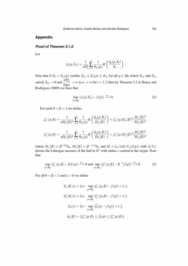
Proof of Theorem 3.1.2.

Let

fn(p,δn) =1

nδdn

n

∑i=1

1

θXi(p)

K

(dg(p,Xi)

δn

).

Note that if δn = δn(p) verifies δ1n ≤ δn(p) ≤ δ2n for all p ∈ M0 where δ1n and δ2n

satisfy δin → 0 andnδd

in

logn→ ∞ as n → ∞ for i = 1,2 then by Theorem 3.2 in Henry and

Rodriguez (2009) we have that

supp∈M0

| fn(p,δn)− f (p)| a.s.−→ 0 (2)

For each 0 < β < 1 we define,

f−n (p,β) =1

nD+n (β)

d

n

∑i=1

1

θXi(p)

K

(dg(p,Xi)

D−n (β)

)= f−n (p,D−

n (β)d)

D−n (β)

d

D+n (β)

d.

f+n (p,β) =1

nD−n (β)

d

n

∑i=1

1

θXi(p)

K

(dg(p,Xi)

D+n (β)

)= f+n (p,D+

n (β)d)

D+n (β)

d

D−n (β)

d.

where D−n (β) = β

1/2dhn, D+n (β) = β

−1/2dhn and hdn = kn/(nλ(V1) f (p)) with λ(V1)

denote the Lebesgue measure of the ball in Rd with radius r centred at the origin. Note

that

supp∈M0

| f−n (p,β)−β f (p)| a.s.−→ 0 and supp∈M0

| f+n (p,β)−β−1 f (p)| a.s.−→ 0. (3)

For all 0 < β < 1 and ǫ > 0 we define

S−n (β ,ǫ) = {w : sup

p∈M0

| f−n (p,β)− f (p)|< ǫ },

S+n (β ,ǫ) = {w : sup

p∈M0

| f+n (p,β)− f (p)|< ǫ },

Sn(ǫ) = {w : supp∈M0

| fn(p)− f (p)|< ǫ },

An(β) = { f−n (p,β)≤ fn(p)≤ f+n (p,β)}


Then, An(β)∩ S−n (β ,ǫ)∩ S+

n (β ,ǫ) ⊂ Sn(ǫ). Let A = supp∈M0f (p). For 0 < ǫ < 3A/2

and βǫ = 1− ǫ3A

consider the following sets

Gn(ǫ) ={

w : D−n (βǫ)≤ ζn(p)≤ D+

n (βǫ) for all p ∈ M0

}

G−n (ǫ) = { sup

p∈M0

| f−n (p,βǫ)−βǫ f (p)|< ǫ3}

G+n (ǫ) =

{supp∈M0

| f+n (p,βǫ)−β−1ǫ f (p)|< ǫ

3

}.

Then we have that Gn(ǫ)⊂ An(βǫ), G−n (ǫ)⊂ S−

n (βǫ,ǫ) and G+n (ǫ)⊂ S+

n (βǫ,ǫ). There-

fore, Gn(ǫ)∩G−n (ǫ)∩G+

n (ǫ)⊂ Sn(ǫ).

On the other hand, using that limr→0 V (Br(p))/rdµ(V1) = 1, where V (Br(p)) de-

notes the volume of the geodesic ball centered at p with radius r (see Gray and Vanhecke

(1979)) and similar arguments those considered in Devroye and Wagner (1977), we get

that

supp∈M0

∣∣∣∣kn

nλ(V1) f (p)Hdn (p)

−1

∣∣∣∣a.s.−→ 0.

Recall that in jgM > 0 and Hdn (p)

a.s.−→ 0. Then for straightforward calculations we

obtained that supp∈M0

∣∣∣ kn

nλ(V1) f (p)ζdn(p)

−1

∣∣∣ a.s.−→ 0. Thus, IGcn(ǫ)

a.s.−→ 0 and (3) imply that

IScn(ǫ)

a.s.−→ 0. �


A Taylor expansion of second order gives

√kn

{1

nζdn(p)

n

∑j=1

1

θX j(p)

K

(dg(p,X j)

ζn(p)

)− f (p)

}= An +Bn +Cn

where

An = (hdn/ζ

dn(p))

√kn

{1

nhdn

n

∑j=1

1

θX j(p)

K

(dg(p,X j)

hn

)− f (p)

},

Bn =√

kn((hdn/ζ

dn(p))−1)

{f (p)+

[(hn/ζn(p))−1]hdn

[(hdn/ζ

dn(p))−1]ζd

n(p)

1

nhdn

n

∑j=1

1

θX j(p)

K1

(dg(p,X j)

ζn(p)

)}

and

Cn =√

kn((hdn/ζ

dn(p))−1)

[(hn/ζn(p))−1]2

2[(hdn/ζ

dn(p))−1]

1

nζdn(p)

n

∑j=1

1

θX j(p)

K2

(dg(p,X j)

ξn

)[ξn/hn]

2


with hdn = kn/n f (p)λ(V1) and min(hn,ζn) ≤ ξn ≤ max(hn,ζn). Note that H6 implies

that hn satisfies the necessary hypothesis given in Theorem 4.1 in Rodriguez and Henry

(2009), in particular

√nhd+4

n → βd+4

d ( f (p)λ(V1))− d+4

2d .

By the Theorem and the fact that hn/ζn(p)p−→ 1, we obtain that An converges to a

normal distribution with mean b(p) and variance σ2(p). Therefore it is enough to show

that Bn and Cn converges to zero in probability.

Note that(hn/Hn(p))−1

(hdn/ζ

dn(p))−1

p−→ d−1 and by similar arguments those considered in Theorem

3.1 in Pelletier (2005) and Remark 3.2.1 we get that

1

nhdn

n

∑j=1

1

θX j(p)

K1

(dg(p,X j)

ζn(p)

)p−→∫

K1(u)du f (p) =−d f (p).

Therefore, by Theorem 3.2.3, we obtain that Bnp−→ 0. As ξn/hn converges to one in

probability, in order to concluded the proof, it remains to prove that

1

nζdn(p)

n

∑j=1

1

θX j(p)

|K2 (dg(p,X j)/ξn) |

is bounded in probability.

By H7, there exits r > 0 such that |t|d+1|K2(t)| ≤ 1 if |t| ≥ r. Let Cr = (−r,r), then

we have that

1

nζdn(p)

n

∑j=1

1

θX j(p)

∣∣∣∣K2

(dg(p,X j)

ξn

)∣∣∣∣ ≤sup|t|≤r |K2(t)|

nζdn(p)

n

∑j=1

1

θX j(p)

ICr

(dg(p,X j)

ξn

)

+1

nζdn(p)

n

∑j=1

1

θX j(p)

ICcr

(dg(p,X j)

ξn

)∣∣∣∣dg(p,X j)

ξn

∣∣∣∣−(d+1)

As min(hn,ζn(p))≤ ξn ≤ max(hn,ζn(p)) = ξn it follows that

1

nζdn(p)

n

∑j=1

1

θX j(p)

∣∣∣∣K2

(dg(p,X j)

ξn

)∣∣∣∣≤

≤(

hn

ζn(p)

)d

sup|t|≤r

|K2(t)|1

nhdn

n

∑j=1

1

θX j(p)

ICr

(dg(p,X j)

hn

)

+ sup|t|≤r

|K2(t)|1

nζdn(p)

n

∑j=1

1

θX j(p)

ICr

(dg(p,X j)

ζn(p)

)


+

(hn

ζn(p)

)d1

nhdn

n

∑j=1

1

θX j(p)

ICcr

(dg(p,X j)

hn

)∣∣∣∣dg(p,X j)

hn

∣∣∣∣−(d+1)

∣∣∣∣∣ξn

hn

∣∣∣∣∣

(d+1)

+1

nζdn(p)

n

∑j=1

1

θX j(p)

ICcr

(dg(p,X j)

ζn(p)

)∣∣∣∣dg(p,X j)

ζn(p)

∣∣∣∣−(d+1)

∣∣∣∣∣ξn

ζn(p)

∣∣∣∣∣

(d+1)

= Cn1 +Cn2 +Cn3 +Cn4.

By similar arguments those considered in Theorem 3.1 in Pelletier (2005), we have that

Cn1p−→ f (p)

∫ICr(s)ds and Cn3

p−→ f (p)∫

ICcr(s)|s|−(d+1)ds.

Finally, let Aǫn = {(1−ǫ)hn ≤ ζn ≤ (1+ǫ)hn} for 0≤ ǫ≤ 1. Then for n large enough

P(Aǫn)> 1− ǫ and in Aǫn we have that

ICr

(dg(X j, p)

ζn(p)

)≤ ICr

(dg(X j, p)

(1+ ǫ)hn

),

ICcr

(dg(X j, p)

ζn(p)

)∣∣∣∣dg(X j, p)

ζn(p)

∣∣∣∣−(d+1)

≤ ICcr

(dg(X j, p)

(1− ǫ)hn

)∣∣∣∣dg(X j, p)

(1− ǫ)hn

∣∣∣∣−(d+1) ∣∣∣∣

ζn(p)

(1− ǫ)hn

∣∣∣∣(d+1)

.

This fact and analogous arguments those considered in Theorem 3.1 in Pelletier (2005),

allow to conclude the proof. �


Denote bn = hdn/(1+ zk

−1/2n ), then

P(√

kn(hdn/ζ

dn −1)≤ z) = P(ζd

n ≥ bn) = P(Hdn ≥ bn, in jgMd ≥ bn).

As bn → 0 and in jgM > 0, there exists n0 such that for all n ≥ n0 we have that

P(Hdn ≥ bn, in jgMd ≥ bn) = P(Hd

n ≥ bn).

Let Zi such that Zi = 1 when dg(p,Xi) ≤ b1/dn and Zi = 0 elsewhere. Thus, we have

that P(Hdn ≥ bn) = P(∑n

i=1 Zi ≤ kn). Let qn = P(dg(p,Xi)≤ b1/dn ). Note that qn → 0 and

nqn → ∞ as n → ∞, therefore

P

(n

∑i=1

Zi ≤ kn

)= P

(1√nqn

n

∑i=1

(Zi −E(Zi))≤1√nqn

(kn −nqn)

).


Using the Lindeberg Central Limit Theorem we easily obtain that (nqn)−1/2

∑ni=1(Zi − E(Zi)) is asymptotically normal with mean zero and variance one. Hence,

it is enough to show that (nqn)−1/2(kn −nqn)

p−→ z+b1(p).

Denote by µn = n

∫

Bb

1/dn

(p)( f (q)− f (p))dνg(q). Note that µn = n qn − wn with

wn = n f (p)V (Bb

1/dn

(p)). Thus,

1√nqn

(kn −nqn) = w−1/2n (kn −wn)

(wn

wn +µn

)1/2

+µn

w1/2n

(wn

wn +µn

)1/2

.

Let (Bb

1/dn

(p),ψ) be a coordinate normal system. Then, we note that

1

λ(Vb

1/dn

)

∫

Bb

1/dn

(p)f (q)dνg(q) =

1

λ(Vb

1/dn

)

∫

Vb

1/dn

f ◦ψ−1(u)θp ◦ψ−1(u)du.

The Lebesgue’s Differentiation Theorem and the fact thatV (B

b1/dn

(p))

λ(Vb

1/dn

)→ 1 imply that

λn

wn

→ 0. On the other hand, from Gray and Vanhecke (1979), we have that

V (Br(p)) = rdλ(V1)(1−τ

6d +12r2 +O(r4)).

Hence, we obtain that

w−1/2n (kn −wn) =

w−1/2n kn z k

−1/2n

1+ zk−1/2n

+w−1/2n τb

2/dn kn

(6d+12)(1+ zk−1/2n )

+w−1/2n kn O(b4/d

n )

= An +Bn +Cn.

It’s easy to see that An → z and w−1/2n b

2/dn kn =

knn−1/2b2/d−1/2n

( f (p)λ(V1))−2/d

(bnλ(V1)

V (Bb

1/dn

(p))

)1/2

, since H6

we obtain that Bn → τ β (d+4)/d/(6d+12) ( f (p)µ(V1))−2/d . A similar argument shows

that Cn → 0 and therefore we get that w−1/2n (kn−wn)→ z+β

d+4d

τ6d+12

( f (p)λ(V1))−d/2.

In order to concluded the proof we will show that

µn

w1/2n

→ βd+4

d

( f (p)λ(V1))(d+2)/d

∫

V1

u21 du L1(p).


We use a second-order Taylor expansion that leads to,

∫

Bb

1/dn

(p)( f (q)− f (p))dνg(q) =

d

∑i=1

∂ f ◦ψ−1

∂ui

|u=0b1+1/dn

∫

V1

ui θp ◦ψ−1(b1/dn u) du

+d

∑i, j=1

∂ 2 f ◦ψ−1

∂ui∂u j

|u=0b1+2/dn

∫

V1

uiu j θp ◦ψ−1(b1/dn u) du

+O(b1+3/dn ).

Using again a Taylor expansion on θp ◦ψ−1(·) at 0 we have that

∫

Bb

1/dn

(p)( f (q)− f (p))dνg(q) = b1+2/d

n

∫

V1

u21 du L1(p)+O(b1+3/d

n )

and by H6 the theorem follows. �

References

Bai, Z. D., Rao, C. and Zhao, L. (1988). Kernel estimators of density function of directional data. Journal

of Multivariate Analysis, 27, 24–39.

Berger, M., Gauduchon, P. and Mazet, E. (1971). Le Spectre d’une Variete Riemannienne. Springer-Verlag.

Boothby, W. M. (1975). An Introduction to Differentiable Manifolds and Riemannian Geometry. Academic

Press, New York.

Butler, R. (1992). Paleomagnetism:Magnetic Domains to Geologic Terranes. Blackwell Scientific Publica-

tions.

Cox, A. and Doell, R. (1960). Review of paleomagnetism, Geological Society of America Bulletin, 71,

645–768.

Devroye, L. and Wagner, T. J. (1977). The strong uniform consistency of nearest neighbor density esti-

mates. Annals of Statistics, 3, 536–540.

Do Carmo, M. (1988). Geometria Riemaniana. Proyecto Euclides, IMPA. 2a edicion.

Fisher, R. A. (1953). Dispersion on a sphere. Proceedings of the Royal Society of London, Ser. A, 217, 295–

305.

Fisher, N. I., T. Lewis and Embleton, B. J. J. (1987). Statistical Analysis of Spherical Data. New York:

Cambridge University Press.

Gallot, S., Hulin, D. and Lafontaine, J. (2004). Riemannian Geometry. Springer. Third Edition.

Garcıa-Portugues, E., Crujeiras, R. and Gonzalez-Manteiga, W. (2011). Exploring wind direction and SO2

concentration by circular–linear density estimation. Prepint.

Goh, A. and Vidal, R. (2008). Unsupervised Riemannian clustering of probability density functions. Lec-

ture Notes In Artificial Intelligence, 5211.

Gray, A. and Vanhecke, L. (1979). Riemannian geometry as determined by the volumes of small geodesic

balls. Acta Mathematica, 142, 157–198.


Hall, P., Watson, G. S. and Cabrera, J. (1987). Kernel density estimation with spherical data. Biometrika,

74, 751–762.

Henry, G. and Rodriguez, D. (2009). Kernel density estimation on Riemannian manifolds: asymptotic re-

sults. Journal of Mathematical Imaging and Vision, 43, 235–639.

Jammalamadaka, S. and SenGupta, A. (2001). Topics in circular statistics. Multivariate Analysis, 5. World

Scientific, Singapore.

Joshi, J., Srivastava, A. and Jermyn, I. H. (2007). Riemannian analysis of probability density functions with

applications in vision. Proceedings of the IEEE Computer Vision and Pattern Recognition.

Love, J. and Constable, C. (2003). Gaussian statistics for palaeomagnetic vectors. Geophysical Journal

International, 152, 515–565.

Mardia, K. and Jupp, P. (2000). Directional Data. New York: Wiley.

Mardia, K. and Sutton, T. (1978). A model for cylindrical variables with applications. Journal of the Royal

Statistical Society. Series B. (Methodological), 40, 229–233.

Parzen, E. (1962). On estimation of a probability density function and mode. The Annals of Mathematical

Statistics, 33, 1065–1076.

Pelletier, B. (2005). Kernel density estimation on Riemannian manifolds. Statistics and Probability Letters,

73, 3, 297–304.

Pennec, X. (2006). Intrinsic statistics on Riemannian manifolds: basic tools for geometric measurements.

Journal of Mathematical Imaging and Vision, 25, 127–154.

Rosenblatt, M. (1956). Remarks on some nonparametric estimates of a density function. The Annals of

Mathematical Statistics, 27, 832–837.

Wagner, T. (1975). Nonparametric estimates of probability densities. IEEE Transactions on Information

Theory IT, 21, 438–440.

Locally adaptive density estimation on Riemannian manifolds - Idescat

Documents

Transcript of Locally adaptive density estimation on Riemannian manifolds - Idescat