Localization of gravity and topography: constraints on the … · 2017-02-27 · both the geoid and...

Geophys. J . Int. (1997) 131,24-44

Localization of gravity and topography: constraints on the tectonics and mantle dynamics of Venus

Mark Simons,l** Sean C. Solomon2 and Bradford H. Hager' Department of Earth, Atmospheric, and Planetary Sciences, Massachusetts Institute of Technology, Cambridge, MA 021 39, USA

E-mail: [email protected] ZDepartment of Terrestrial Magnetism, Carnegie Institution of Washington, Washington, DC 20015, U S A

Accepted 1997 April 24. Received 1997 March 10; in original form 1996 July 15

SUMMARY We develop a method for spatio-spectral localization of harmonic data on a sphere and use it to interpret recent high-resolution global estimates of the gravity and topography of Venus in the context of geodynamical models. Our approach applies equally to the simple spatial windowing of harmonic data and to variable-length-scale analyses, which are analogous to a wavelet transform in the Cartesian domain. Using the variable-length-scale approach, we calculate the localized RMS amplitudes of gravity and topography, as well as the spectral admittance between the two fields, as functions of position and wavelength. The observed admittances over 10 per cent of the surface of Venus (highland plateaus and tessera regions) are consistent with isostatic compensation of topography by variations in crustal thickness, while admittances over the remaining 90 per cent of the surface (rises, plains and lowlands) indicate that long- wavelength topography is dominantly the result of vertical convective tractions at the base of the lithosphere. The global average crustal thickness is less than 30 km, but can reach values as large as 40 km beneath tesserae and highland plateaus. We also note that an Earth-like radial viscosity structure cannot be rejected by the gravity and topography data and that, without a mechanical model of the lithosphere, admittance values cannot constrain the thickness of the thermal boundary layer of Venus. Modelling the lithosphere as a thin elastic plate indicates that at the time of formation of relief in highland plateaus and tesserae, the effective elastic plate thickness, K , was less than 20 km. Estimates of T, at highland rises are consistently less than 30 km. Our inability to find regions with T, > 30 km is inconsistent with predictions made by a class of catastrophic resurfacing models.

Key words: convection, geoid, gravity, tectonics, Venus, wavelets.

INTRODUCTION

The terrestrial planets lose their internal heat, acquired during planet formation and produced by radioactive decay, through subsolidus mantle convection (e.g. Schubert, Turcotte & Oxburgh 1969; OConnell & Hager 1980; Sleep & Langan 1981; Basaltic Volcanism Study Project 1981). Our understanding of the dynamics of mantle convection and its resulting surface manifestations has relied heavily on the analysis of gravitational and topographic data (e.g. Kaula 1968; McKenzie 1977a). For Earth, the surface manifestations of mantle convection (e.g. mountain building and rifting) are dominated by plate tectonics and the formation and evolution of continents

*Now at: Division of Geological and Planetary Sciences, California Institute of Technology, Pasadena, CA 90024, USA.

(e.g. Wilson 1965; McKenzie 1967; Jordan 1978; Burchfiel 1983). When viewed globally, long-wavelength geoid anomalies on Earth reflect principally the effects of subduction processes and lower-mantle structure (Crough & Jurdy 1980; Hager 1984; Hager et al. 1985). At shorter wavelengths, the thermal structure of the lithosphere, crustal thickness variations, glacial unloading and upwelling of hot mantle have important signatures (e.g. Walcott 1972; Parsons & Richter 1980; Sleep 1990; Simons 1995).

Although Venus and Earth are similar in size, density and bulk composition (e.g. Phillips & Malin 1983), radar images of the surface of Venus obtained by the recent Magellan mission show no evidence for global plate tectonics (Solomon et al. 1991, 1992). Thus, the surface manifestations of mantle convection are quite different on the two planets, a result plausibly attributed to the high temperatures and extreme

24 0 1997 RAS

at California Institute of T

echnology on June 5, 2013http://gji.oxfordjournals.org/

Dow

nloaded from

http://gji.oxfordjournals.org/

Tectonics und mantle dynamics of Venus 25

dryness of the Venus surface (McKenzie 1977b Phillips & Malin 1983; Phillips et al. 1991; Kaula 1990, 1995). The composition of surface rocks, as determined at a handful of Venera and Vega landing sites, is nonetheless broadly similar to that of oceanic basalts (Surkov et al. 1983, 1984, 1986, 1987). For Earth-like abundances of the heat-producing elements U, Th and K, simple scaling of terrestrial heat loss to Venus predicts an average heat loss of about 70 mW m-’ (Solomon & Head 1982). Somewhat lower values (50-55 mW m-2) for the average heat flux have been obtained from thermal models and the assumption of chondritic heat production (Phillips & Malin 1983). We must ask how Venus, with no evidence for plate tectonics, loses its heat. Of particular interest is our ability, or lack thereof, to estimate the average thickness of the surficial thermal boundary layer (TBL) of Venus.

Turcotte (1993) has proposed that the TBL is 300 km thick on Venus on the basis of high geoid-to-topography ratios (GTRs) (e.g. Smrekar & Phillips 1991), a large effective thickness of the elastic lithosphere, and the suggestion that the lithosphere has conductively cooled for about the last 500 Myr. This last suggestion was motivated by the distribution and generally well-preserved states of impact craters on Venus, consistent with the view that most of the surface of Venus has been unmodified by significant volcanism or deformation for approximately half-a-billion years (Phillips et al. 1991, 1992; Schaber et al. 1992; Strom, Schaber & Dawson 1994). Turcotte (1993) interpreted the crater characteristics as evidence for episodic plate tectonics, whereby the global lithosphere cools conductively for several hundred million years, thickens to a value beyond that expected by marginal stability analysis, and then founders in a planet-wide event of short duration (catastrophic overturn). In proposing a similar model, Parmentier & Hess (1992) drew attention to the depleted mantle layer that should develop after partial melt extraction in a system lacking a mechanism for wholesale lithospheric recycling. In their model, the bottom of the lithosphere is negatively buoyant and would periodically delaminate. If the assumption that scaling of global heat loss from the Earth is valid, a 300-km-thick TBL does not permit sufficient heat flux, so there is a need for episodes of greater-than-average heat flux (e.g. Turcotte 1993). In contrast, Solomon (1993) proposed that the surface of Venus has experienced a monotonic but geologically rapid decline in tectonic activity due to secular cooling and the strongly non-linear dependence of crustal rheology on temperature and differential stress. Without a catastrophic resurfacing event, this model requires a thinner lithosphere at present to satisfy the predicted average heat loss. Thus, an important question is whether an analysis of surface tectonics and geophysical observations can distinguish between a 300-km-thick TBL and one several times thinner.

We address the questions of topographic support and TBL thickness by means of gravity and topography data obtained during the Magellan mission (Ford & Pettengill 1992; Konopliv & Sjogren 1994, 1996). In this study we consider both the geoid and free-air gravity representations of the gravity data. Gravity and topography are typically related through an admittance function, defined as the variation in gravity (or geoid) divided by the variation in topography, with its sign and amplitude able to vary as a function of position and wavelength.

Before the Magellan mission (Saunders et al. 1990; Saunders & Pettengill 1991), tracking data from the Pioneer Venus

Orbiter (PVO) indicated that the geoid height and topography of Venus are highly correlated on a planetary scale (Sjogren et al. 1983; Kiefer et al. 1986), but global analyses carried out with these data were limited to spherical harmonic degree 18 and less, and only global averages of the admittance were obtained. Several studies made use of line-of-sight (LOS) accelerations of the PVO spacecraft over limited geographic areas on Venus to demonstrate that geoid height and topography correlate on shorter scales than could be represented with the global spherical harmonic fields then available, but such studies were restricted to a few selected regions (e.g. Herrick, Bills & Hall 1989; Smrekar & Phillips 1991; Grimm & Phillips 1991, 1992). More recently, with global coverage of the gravity field at generally improved resolution, most investigators have used spherical harmonic representations (e.g. Simons, Hager & Solomon 1994; Grimm 1994; Phillips 1994; McKenzie 1994; Schubert, Moore & Sandwell 1994; Smrekar 1994), although some have also employed regional gravity fields derived directly from the LOS tracking data (e.g. Phillips 1994; Smrekar 1994).

Many analyses and interpretations of the gravity and topography of Venus depend strongly on the assumptions made during field manipulation. Both purely spatial and purely spectral techniques have been employed. While the spectral analysis of these global data sets is both tractable and physically meaningful, the spatial juxtaposition of distinct geological provinces and geodynamic processes suggests that spectra and their transfer functions should vary with position. As with Fourier series for Cartesian geometry, however, spherical harmonic functions are not spatially compact and are therefore not well suited to regional analysis. The spatial non-stationarity intrinsic to geophysical observations thus motivates us to consider new spectral methods. In particular, we seek techniques to estimate the frequency content of a signal as a function of position, generically termed localization methods.

Non-stationary spectrum-estimation techniques are not new. Wavelets and other multiresolution methods are now common for time-series analysis and image processing (e.g. Daubechies 1992). Localization techniques exist for analysing both 1- and 2-D data, but available techniques are designed for a Cartesian domain (however, see Schroder & Sweldens 1995). We introduce here a technique for spatio-spectral localization of data on a sphere. In the spirit of Cartesian wavelet transforms, our goal is to estimate non-stationary frequency spectra. Because this approach is new, the development of the method is given in detail along with a synthetic example. The multiresolution approach distinguishes features which have large amplitudes but are limited in spatial extent from those which are truly long-wavelength and cyclic in character, that is we make the crucial distinction between a characteristic length-scale and a characteristic wavelength. This distinction is epitomized by the delta function, which has a characteristic length-scale of zero but incorporates the entire spectral domain.

Our localization method relies on spatial windowing of a data field using smooth windows with characteristic length- scales that can be functions of the harmonic degree being considered. This spatial windowing can be viewed either as spectral convolution of the window with the data or as a projection of the data onto a set of basis functions formed as products of a single spherical harmonic and the window. In addition, the spectral-domain perspective illuminates potential spatial and spectral aliasing problems that arise if one were to

0 1997 RAS, GJI 131, 24-44



Dow

nloaded from


26 M . Simons, S . C . Solonzon und B. H. Huger

choose arbitrary spatial or spectral windows when analysing the medium to long wavelengths characteristic of global data sets and models. In particular, this approach exposes the limits to which we can simultaneously analyse both the spatial and the spectral behaviour of the gravity and topography given the finite spectral resolution of spherical harmonic fields.

On the basis of an early harmonic model of the global gravity field, and a technique related to that developed here, it has been shown that crustal thickness variations can explain the observed geoid and topography over only a small portion of the surface of Venus, while fields for the remainder of the planet are consistent with a model in which variations in gravity and topography result primarily from convection- induced vertical tractions at the base of the lithosphere (Herrick & Phillips 1992; Simons et al. 1994). In this paper, we use our localization method to broaden and refine these conclusions.

Specifically, we calculate the localized root-mean-squared (RMS) amplitudes of the geoid and topography of Venus as functions of position and wavelength, as well as the spectral admittance between the two fields. Many regions on Venus have very high admittance values, a result cited by others as evidence for the lack of an Earth-like increase with depth of mantle viscosity (e.g. Kiefer et al. 1986; Kiefer & Hager 1991a; Phillips 1990; Smrekar & Phillips 1991). On the basis of previous mantle-flow models, however, we argue that such a conclusion cannot be rigorously made. The high admittance values have also been invoked as support for a 300-km-thick thermal boundary layer on Venus, over twice the thickness of the thermal boundary layer in Earth’s oceanic regions. We argue instead that, because of the sensitivity of the gravity field to the distribution of density anomalies and viscosity variations, admittance values alone cannot be used as constraints on the thermal boundary layer structure of Venus, that there is no reason based on this evidence to favour a TBL thickness of 300 km over a more Earth-like 50-150 km, and that estimates of T, are in fact consistent with a TBL less than 150 km thick.

Our results force us to address the issue of the evolution of the style of surface deformation on Venus over the past half- billion years. As in Simons et al. (1994), we argue that the admittance values in regions that are well described by a static compensation model, that is the highland plateaus and tesserae, represent fossils of a now extinct regime. The failure of static models for the remaining 90 per cent of the surface implies that admittance analyses that rely on spatially derived GTRs (e.g. Smrekar & Phillips 1991; Grimm & Phillips 1991, 1992; Kucinskas & Turcotte 1994; Schubert et al. 1994; Moore & Schubert 19951, that is for which a single apparent depth of topographic compensation (ADC) over a finite band of wavelengths is assumed, either in the processing or in the interpretation, may give misleading results when applied to regions with inherently dynamic signatures. The method used here identifies those few regions where a single ADC does explain the observations well. However, a single ADC can be inferred only after completion of the full spectral analysis and should not provide the assumption on which the processing or the interpretation of gravity and topography data is based (Simons et al. 1994; McKenzie 1994).

A BRIEF GUIDE TO VENUS SURFACE TECTONICS

The surface of Venus includes a wide range of geological structures. The global hypsometric profile is unimodal, unlike

the bimodal distribution for Earth (Pettengill et (I!. 1980), reflecting the lack of an ocean/continent dichotomy. On the basis of elevation (Fig. l), the surface can be divided into highlands, lowlands and plains (Masursky et al. 1980). Highlands are generally further subdivided into plateaus and rises, depending on their long-wavelength topographic cross-sections.

The largest of the highland terrains is Aphrodite Terra, which straddles the equator for half the circumference of the planet. Western Aphrodite Terra consists of Ovda and Thetis Regiones, steep-flanked highland plateaus approximately 3 km above the planetary mean radius and characterized by pervasive, dominantly compressive deformational features (Solomon et al. 1991, 1992). In contrast, eastern Aphrodite Terra encompasses a broad rise, Atla Regio, topped by rift valleys and large volcanoes, with little evidence for compressional deformation (Solomon et al. 1991, 1992; Senske, Schaber & Stofan 1992). Beta and Eistla Regiones (Fig. 1) are each similarly characterized by a topographic rise, large volcanoes and rifting (McGill et al. 1981; Solomon et al. 1991, 1992; Senske et al. 1992; Grimm & Phillips 1992). Frequently associated with regions of rifting and extension are chains of coronae, circular to ellipsoidal features consisting of an annulus of deformed terrain and often an elevated interior (Pronin & Stofan 1990; Squyres et al. 1992a). O n the basis of their geometry and the common occurrence of interior volcanic deposits, coronae generally have been held to be surficial expressions of cylindrical mantle upwelling, but the details of corona formation and evolution are not known (e.g. Squyres et al., 1992a; Sandwell & Schubert 1992; Stofan, Smrekar & Bindschadler 1995; Janes & Squyres 1995; Koch & Manga 1996).

Ishtar Terra (Fig. l), which encompasses several mountain belts and blocks of highly deformed terrain, is the second largest compressionally deformed highland (Barsukov et al. 1986; Basilevsky 1986; Pronin 1986; Solomon et al. 1991, 1992; Kaula et al. 1992). Western Ishtar Terra consists of the Lakshmi Planum plateau, approximately 2000 km in dimension and 3 to 4 km in elevation, covered by volcanic plains. The plateau is surrounded by a ring of mountains which reach a maximum elevation of 11 km at Maxwell Montes (Fig. 1). Ishtar Terra has been variously attributed to local mantle upwelling, local mantle downwelling, or a distant source of stress (e.g. Pronin 1986; Bindschadler & Parmentier 1990; Bindschadler, Schubert & Kaula 1990 Grimm & Phillips 1991). In addition to Aphrodite and Ishtar Terrae, there are many smaller highland plateaus. Among these are Alpha and Tellus Regiones (Fig. l), which are steep-sided, complexly deformed terranes, or tesserae, with lateral dimensions of about 1000 km (Solomon & Head 1991; Solomon et al. 1992; Bindschadler et al. 1992a; Hansen & Willis 1996).

Plains and lowlands, the lowest of which are Atalanta and Lavinia Planitiae (Fig. l ) , lie between the highland terrains and make up most of the surface of Venus. Ridge belts, compressional features with hundreds of metres of relief and dimensions of up to several thousand kilometres in length and hundreds of kilometres in width, are frequently associated with the lowest regions of the planet (Zuber 1990 Zuber & Parmentier 1990; Solomon et al. 1992; Squyres et al. 1992b). The plains are generally interpreted to be covered by volcanic flow deposits on the basis of a variety of volcanic landforms (e.g. Head et al. 1991, 1992; Guest et al. 1992).

0 1997 RAS, GJI 131, 24-44



Dow

nloaded from


-2 -1 0 1 2 3 4 Elevation (km)

7

Figure 1. A harmonic expansion of elevation with respect to a 6051-km-radius sphere (here shown to degree and order 120) (Rappaport & Plaut 1994), with major physiographic provinces labelled for reference. Contours every 1 km; elevations 20.5 km and 5 -0.5 km shown by thick and thin lines, respectively. Winkel Tripel projection centred at 60"E.

Figure 2. Global map of geoid model MGNPl2OPSAAP (Konopliv & Sjogren 1996). Contours every 20 m, with geoid height 2 10 m and 5 - 10 m shown by red and blue lines, respectively. Unless stated otherwise, all global maps show highland rises lightly shaded and highland plateaus and tesserae darkly shaded (from Price & Suppe 1995; Price et al. 1996). Winkel Tripel projection centred at 60"E.

O 1997 RAS, G J l 131, 24-44



Dow

nloaded from


Figure 4. Residual geoid, We'(,), generated by removing that part of the geoid which is linearly related to topography in a degree-by-degree global sense. Contours every 20 m, with Nres(C2) 2 10 m and 5 - 10 m indicated by red and blue lines, respectively.

0 1997 RAS, G J I 131, 24-44



Dow

nloaded from


Tectonics and rnantle dynamics of Venus 27

function, P , . The P I spectrum is inconsistent with a single ADC, although there is a suggestion in Fig. 3 that an ADC of about 30 km fits the data for harmonic degree 12 40. Beyond l ~ 8 0 , PI approaches zero, presumably an artefact of the damping applied during the construction of the harmonic gravity model.

We can construct a residual, or zero-correlation, geoid by removing a synthetic field derived by multiplying each degree of the topography by P , at that degree. The fi, spectrum shows some physically unrealistic fluctuation from degree to degree. While we could attempt to fit a smooth curve to this spectrum, our conclusions would be unaffected by this smoothing. From the residual map (Fig. 4), we see that tesserae and highland plateaus correlate strongly with those regions predicted (using P , ) to be overcompensated (that is regions associated with positive geoid anomalies in the original field and with negative geoid anomalies in the residual field). Specifically, the admittance calculated in this way predicts topography which is overcompensated in Ishtar Terra and western Aphrodite Terra and undercompensated at many highland rises, plains and lowlands (Fig. 4). The misfit of the large-scale features stems from the spatial combination of different modes of compensation at long wavelengths. While the residual anomaly is, by definition, uncorrelated with topography when viewed spectrally in a global sense, we see a high correlation when viewed locally (Fig. 4). This apparent contradiction arises because topography and the residual geoid are positively correlated for half the planet and negatively correlated for the other half. The residual anomaly is striking because of the correlation of the residual anomaly with the tectonic regionalization. Since the global admittance predicts topography that is overcompensated in tesserae and plateaus and undercompensated at highland rises, plains and lowlands, we conclude that the geoid signal from the latter regions dominates the total global signal.

In order to progress beyond the purely spectral or purely spatial approaches, we must localize the geoid and topography data in the two domains simultaneously. Historically, investi- gations of geoid-topography relations on Venus employed GTRs, spatial estimates of the covariance of geoid height and surface elevation over a finite region (e.g. Smrekar & Phillips 1991; Grimm & Phillips 1992; Kucinskas & Turcotte 1994; Schubert et al. 1994; Moore & Schubert 1995; Moresi & Parsons 1995). GTRs have been calculated using two different approaches. In the first, the LOS data are combined with the topographic data to determine the best single ADC. The ADC

By combining topographic information with geological maps of highland plateaus and tesserae we may define a simple global tectonic regionalization. Harmonic topography more elevated than 0.5 km above the planetary mean radius is divided, on the basis of the global geological maps of Price & Suppe (1995) and Price et ul. (1996), into highland plateaus and tesserae or highland volcanic rises (indicated by dark and light shading, respectively, on all subsequent global maps). Regions at lower elevations may be grouped together as plains and lowlands. While this regionalization is overly simplified with respect to geological structures, we shall see that it is adequate for the treatment of localized admittances.

GLOBAL GEOID, TOPOGRAPHY A N D ADMITTANCE OF VENUS

We make use of a spherical harmonic model of the geoid, or equivalently the gravity field, of Venus that includes LOS tracking data from both the Magellan and Pioneer Venus missions and has a maximum degree and order of 120 (Konopliv & Sjogren 1996). The spatial rendition of this geoid model is shown in Fig. 2. This solution includes data obtained during tracking of the Magellan spacecraft in a nearly circular orbit with an apoapsis of about 550 km and a periapsis of about 180 km (Konopliv & Sjogren 1994). The spherical harmonic expansion of the topography is taken from values gridded every 0.25" in latitude and longitude (Ford & Pettengill 1992) and is complete to degree and order 360 (Rappaport & Plaut 1994).

The close association of highlands and geoid highs is remark- able, and leads to the hypothesis that the geoid arises from either isostatic (e.g. Haxby & Turcotte 1978) or dynamic (e.g. Richards & Hager 1984) compensation of topography. Here, isostatic compensation refers to the balancing of topographic loads with density variations at depth. These variations can be either at discrete interfaces, such as the crust-mantle boundary, or volumetrically distributed, such as contributions from the thermal and chemical structure of the interior. In contrast, dynamic compensation refers to surface topography supported by stresses from mantle flow.

We begin our analysis of topographic compensation on Venus with a purely spectral approach. In Fig. 3 we show RMS amplitude versus spherical harmonic degree for both geoid and topography. We also show the degree correlation between the two fields, as well as the least-squares estimate of the degree-dependent global geoid/topography admittance

1 50 40

5 30 I

E 20 4: 10

0

10 100 lo loo -'lHarmonic Degree, / Harmonic Degree, /

1 10 100 1 Harmonic Degree, /

Figure 3. Left: RMS amplitude spectra, s,, of geoid (m) and topography (km) represented by circles and crosses, respectively. Middle: geoid/ topography admittance, p,, with 1u errors. For reference, we show theoretical curves for Airy compensation at depth D (in km). Right: degree correlation, i,, between geoid and topography for the observed geoid (circles); 98 per cent confidence limits are shown by the solid lines.

0 1997 RAS, GJI 131, 24-44



Dow

nloaded from


28 M . Simons, S. C. Solomon and B. H. Huger

is then converted to a GTR estimate (e.g. Smrekar & Phillips 199 1 ) . This approach relies on the premise that topography may be treated as if locally compensated at one depth and that the transfer function between the geoid and the topography is independent of wavelength over the band considered. If incorrect, as suggested by the analysis of the previous section, these premises can lead to erroneous conclusions. However, despite these shortcomings, Smrekar & Phillips (1991) were able to classify the highlands into two groups depending on the value of their GTRs, a distinction that still remains (Fig. 4). The second approach to estimating a GTR is to use a gravity model gridded in the spatial domain (e.g. Kucinskas & Turcotte 1994; Moore & Schubert 1995). A similar procedure can be used to calculate GTRs from model calculations (e.g. Moresi & Parsons 1995). However, given that a full gravity model is available, information is lost by collapsing the full wavelength- dependent transfer function into a single number. Furthermore, GTR analyses for both Earth and Venus have either included all wavelengths of the data (Smrekar & Phillips 1991) or were conducted after first bandpassing the geoid and topography to isolate a single wavelength band (Sandwell & Renkin 1988; Sandwell & MacKenzie 1989; Kucinskas & Turcotte 1994; Moore & Schubert 1995). Given the red spectra of the original fields, the estimated GTR is then dominated by the longest wavelengths passed. In addition, spectral bandpassing followed by spatial localization can result in spatial aliasing (Sandwell & Renkin 1988). Finally, since the gravity data are currently available only as a finite set of spherical harmonic coefficients, there is an undesirable arbitrariness involved when such data are used in a purely spatial sense, as when calculating a GTR (for example choosing how many points to use and deciding which wavelength band to consider).

The admittance, while similar to the GTR, is in the wave- number domain and can therefore vary with wavelength. The approach taken here is first to localize in space, then in frequency, while only considering wavelengths less than the scale of spatial localization. Although some long-wavelength bias still exists due to the spatial windowing of data having red spectra, this bias is considerably less than with the GTR technique, and is overt. Furthermore, as long as comparisons are made with models that have had the same windowing applied to them, we are not seriously affected by this bias. Windowing the models in the same manner as the data is also important because we are seeking horizontal variations in model parameters and we normally interpret the data by means of forward models that vary with depth but not horizontal position. While windowing has a minimal effect on forward models of Airy compensation (local compensation by variations in the depth to an interface separating materials of different density), it has a strong effect on regional compensation models (with finite T,).

SPATIO-SPECTRAL LOCALIZATION O N A SPHERE

We develop a localization procedure for the spherical domain in the context of localizing data a t either fixed or variable length-scales. The latter application involves spatial multiplication of the data with a window whose length-scale is pro- portional to the wavelength being considered. The windowed field is transformed into the spectral domain as a convolution, using spherical harmonics, in order to take full advantage of

known harmonic coupling relations. The localized data can be used to estimate the position- and wavelength-dependent correlation and transfer function between two global fields. The localization transform proposed here is fully invertible by spatial averaging of the localized data.

The localization transform

Following the normalization and phase conventions of Edmonds ( 1957) and Varshalovich, Moskalev & Kjersonskii (1988), we define a field A(Q) on a spherical domain 0 = (0,d) by

and Pi, is an associated Legendre polynomial of degree 1 and order rn, defined in terms of the Legendre polynomials Pi by

a m U P,,(cos 0) = (sin Qm- PI (C0S 01, (d cos 0), ( 3 )

such that

(4) Each spherical harmonic X,(Q) is fully normalized such that

( 5 )

where the integration is over the entire spherical surface, the asterisk denotes complex conjugation, and, unless otherwise specified, 1 = 0, 1 . . . 00 and m = - 1, - 1 + 1, . . . , 1. Each coefficient a,, is defined by

f

and we note that Y,*,(Q) = ( - )mx-rn(Q) and a&, = ( - )mu, -m. Defining a window function

w(Q) = 1 wfrn E;rn(Q) 9

y(Q) = W(Q)A(Q) = C $lm Xrn(Q) >

(7 ) Im

and the spatially localized version of A by

(8) Im

the coefficients of the localized field are r

It is worth emphasizing that Y and $J~,,, correspond to a window of a given length-scale and position. A different length-scale or position would yield a different set of $,,s. Furthermore, we have not specified the character of the window; the development applies to both multiresolution windows, such as those used here, and spatially complex geographical windows (such as an ocean-continent function).

For comparison with the wavelet approach, we rewrite eq. (9) as the inner product of the data with the localized basis

0 1997 RAS, G J I 131, 24-44



Dow

nloaded from


Tectonics and mantle dynamics of Venus 29

or equivalently,

and we have assumed that W(Q) is real-valued. Care must be taken to ensure that Xlm(Q) has zero mean so that we measure the first moment of our signal without bias from the zeroth moment (e.g. Chui 1992; Daubechies 1992). In addition, to maintain consistency across degrees, we require that W(Q) have a mean amplitude of 1, i.e. that

's W(Q)dQ=l 471

Alternatively, for analysis with a fixed length-scale window, one could require that W(Q) have a maximum amplitude of 1, analogous to classical windowing and the short-time window Fourier transform. The implementation of these constraints is addressed later.

Returning to the form used in eq. (9), and using eqs ( 1 ) and (7), we write

I j l m = 1 a l l m l W i 2 m z Y;lml(Q)Y;2m2(Q)Y,*,(Q) dQ. (13) h m 1 b m Z s

The integral of the product of the three spherical harmonics is evaluated with Wigner 3-j symbols in conjunction with the appropriate selection rules (e.g. Varshalovich et al. 1988), where

(21, + 1)(21, + 1) ... (21, + 1) C11t2...tn = I 471

The brackets in eq. (14) denote the Wigner 3-j coefficients. To be non-zero-valued, the 3-j coefficients must satisfy the conditions that

11, - I21 I 1 I 11 + 1 2 , (16)

l m l l s 4 , l m 2 1 ~ 1 2 , ImIsE (17)

m, + m, + m = 0 , (18) where eq. (16) is commonly known as the triangle inequality. We also note that

and

and

[11 + I , + l lodd - (; ; J=o.

( 2 2 )

If a window (for example the continent-ocean function, a spherical cap or a degree-dependent window) is expanded into spherical harmonics, it is straightforward to calculate the coefficients of the windowed field.

For any window, we need to define a reconstruction algorithm that maps the localized coefficients back to the original field, or equivalently to coefficients of the original field. As demonstrated in Appendix A, we accomplish this by averaging over all possible positions and rotations of the window, which can be written as

where R represents the three Euler angles (a, p, y ) and dR = da sin p dp dy. For axisymmetric windows, we can eliminate the a rotation and the reconstruction becomes

We now address the limitation imposed by starting with a spectrally truncated data set on our ability to analyse a windowed field spectrally. Let Lobs be the highest harmonic degree for which an observed field has significant spectral power. If the window can be expressed in terms of a finite number of coefficients with a maximum degree Lwi, then from the triangle inequality (eq. 16) we find that the degree 1 coefficients of the windowed field receive contributions from data coefficients with lI I 1 + I,. We must ensure that we do not localize a t an I that is sufficiently large such that we are sensitive to data with 1, > lobs. Labelling the critical 1, as Lnyq and recognizing that 1, never exceeds Lwin, we find

which can be regarded as a spherical equivalent of the sampling theorem for localized functions, and is illustrated in Fig. 5. Recognizing that increasing spatial localization increases Lwi,, we must consider eq. ( 2 5 ) when designing windows. We emphasize that a truncated harmonic representation of a data field can never be localized at the highest available degree-a manifestation of the sampling theorem. To attempt to localize

Spatial Spectral

Position, SZ

a

L&

L

L&

Figure 5. The localization operation can be viewed as a spatial multiplication (left) or a spectral convolution (right).

0 1997 RAS, G J I 131, 24-44



Dow

nloaded from


30 M . Simons, S. C. Solomon and B. H. Hagger

at 1 > lnyq involves convolving window coefficients with zero- valued data coefficients, and is therefore the same as convolving the data with a truncated window expansion. However, we can increase the maximum spectral resolution of the localized field, L,,,, by decreasing our spatial resolution. The definition of L,,, is obviously valid both for scalable windows and for arbitrary windows such as a continent-ocean function or another geographic window.

We cannot generate information, only move it around. If the spherical harmonic representation of a global data field can be regarded as having full spectral resolution, then the convolution perspective emphasizes that localization produces spatial resolution at the expense of spectral resolution. Since the basis functions are neither orthogonal nor linearly independent, the spectral estimate at a given spatial location is correlated to the estimate a t a neighbouring point. Similarly, the spectral estimate at a given degree is correlated to the estimate at a neighbouring degree.

Localized field statistics

The linear transfer function between two fields A(R) and B(R) (e.g. gravity and topography) can be written as

B(R) = F(R, R’)A(R’) dR’ s,, Typically, we want to estimate F . Classically, F is restricted to be isotropic, that is it depends on A, the separation distance between R and R’, and further, A and B are assumed to be stationary, so that F is independent of position. These assumptions result in

r B(R) = j F(A)A(R‘) dR’

a’

In contrast, here we permit F(A) to vary spatially using the representations of A and B localized at Ro, and we assume the relationship

r(szo, n) = F(R~ , A ) Y ( R ~ , R’) m, (28) s,. where r is the spatially localized version of B.

localized fields can be written as In Appendix B we show that the cross-covariance of two

where y I m is a harmonic coefficient of r. Using eq. (29), we define, respectively, the RMS amplitude

of Y, and the correlation, transfer function (admittance) and error on the admittance between Y and r as

and

(33)

In subsequent sections, we make use of these localized estimates, the global average of the local estimates, indicated by an overbar (e.g. si), and the non-localized or global estimates, indicated by a hat (e.g. sl). Our analysis does not include a discussion of the uncertainties in the derived statistical estimates or in the original gravity and topography data. Only the formal error in the transfer function between two localized fields is presented here. While this is the error typically presented for two fields with independent harmonic coefficients free of errors, our localized coefficients both are correlated and themselves contain errors, so our error for the transfer function is an underestimate.

Window design

We use a window that is generically defined to be smooth and to scale with wavelength. Here we consider only isotropic windows (that is that depend only on Q) centred at the pole (Q = 0). This restriction can be generalized to other locations by a simple rotation of the coordinate system. Noting that pole-centred isotropic windows only have mz = 0 terms, and using eq. (18) we find that m1 = m, and eq. (21) becomes

We use eqs (29) and (34) under the restrictions that

1 =o, 1, ... , Lnyq,

m=0, 1, ..., 1 ,

(341

1, = max(m, 11- LwinI), ... > min(Lbs, 1 + Lwm) >

1, = 11- Ill, I1 - 1,I + 1, ... , min(l+ I , , L,,,),

(37)

( 3 8 )

where we have limited consideration of $ l m to I > Lwin, which as will be shown later is desirable for other reasons.

We desire a window that minimizes Lwin, the maximum degree needed for accurate representation of the window. This choice reduces potential spectral bias problems incurred from the convolutions intrinsic to the localization transform. Furthermore, the gravity data sets considered here impose severe Nyquist restrictions, which are ameliorated by using the most spectrally compact or spatially smooth window possible. In addition, from a practical perspective, minimizing Lwin reduces computation time significantly.

We use a scalable window based on a spherical cap, defined as

1, for QSQ,

0, for e > 8,’ W(Q, I ) = (391

where 0 I €J I .n, 0, = n/ Jm, and I s = l/L, where the scaling parameter, f, 2 1, is the number of wavelengths, 3, [where ,I = 2 n R / , , h ~ T ] , that fit in the window. The spherical analogue to a Cartesian boxcar, a cap has many well- known disadvantages. However, the window we use has only the first LWj, coefficients of the harmonic expansion of the cap window, where Lwin is the nearest integer less than or equal to I,. This choice of Lwin corresponds to keeping the coefficients within the first lobe of the spectrum of a spherical cap. At

0 1997 RAS, GJ1 131, 24-44



Dow

nloaded from


Tectonics and mantle dynamics qf Venus 31

1 = L,,,. LW,, 2 L,,,/f,, and using eq. (25) we find I

This is written as an approximation since Lwin and L,,, must be integer-valued.

We must also guarantee that our basis function should have zero mean, i.e.

X,,(R) dR = 0 ,

or more explicitly for a pole-centred window,

To satisfy this relation, it is sufficient (and possibly more restrictive than necessary) to require w , ~ = , , ~ = 0. We accomplish this by imposing I , < 1 . From eq. (40) we find that for Lobs = 70 and f , = I, L,,, = 35, and for Lobs = 120 and fs = 2, L,,, = 80. Obviously, f , = 1 provides higher spatial resolution than with &=2. However, when analysing data with noise, it is desirable to minimize potential bias by using f , > 1, thereby localizing at length-scales longer than the wavelength under consideration.

Examples of windows and their spectra are shown in Fig. 6. In addition, examples of W(B, Lwin), E;, and X,, are shown for I = 12 and f , = 1 in Fig. 7. As previously mentioned, whereas the spectrum of a spherical cap has multiple side lobes, our windows incorporate only coefficients within the first central lobe. As the windows become tighter spatially, the central lobe widens and, in the limit of a delta function, gives a flat spectrum, that is perfect spatial resolution with no spectral resolution.

From Fig. 7 we see that a subset of the X,,(R)s are nearly zero-valued. This behaviour arises because our windows are pole-centred, and for a given 1, E;,(R) has decreasing power near the pole with increasing m. We use this fact to reduce computation by modifying eq. (36) to

m=O, 1, ... M,,,, (43)

150 I I I I 1

0 15 30 45 8, deg

60 75 90

1 oo 10' Harmonic Degree, i

Figure 6. Spatial (top) and spectral (bottom) representations of W(f3, Lwi,) for Lwin = 4, 8 and 16 are shown by the solid, dash-dotted and dashed lines, respectively.

-1 ' I 1 O O h -1

a W -50 1

0 15 30 45 60 75 8, deg

90

Figure 7. W(0, L,,,) (top), and latitudinal profiles of &,,(e, 0) (middle) and X,,(O, 0) (bottom) for 1 = 12 and ,f, = 1 (Lmn = 1 1 ) .

where we have neglected all X,,(R)s having a maximum amplitude relative to the maximum amplitude of Xfo(R) less than a specified threshold, here chosen to be 0.01. An increase in f , will result in an increase in M,,,.

The harmonic expansions of the windows are derived in the standard fashion, where

(44)

Since E;,(R) terms do not depend on 4, we rewrite eq. (44) explicitly in terms of Legendre polynomials as

wIzO(Lwin) = 4- jz w(0, Lwin)Plz(cos 0) sin 0 do . 0

(45)

For an arbitrary window, eq.(45) is solved by numerical integration. However, using the identity

the coefficients for a cap with unit amplitude can be calculated analytically, whereby

w:o(Lwin) == ~/;ICPO(COS ~ c ) - P~(COS Q ~ ) I (47) and

cp,z-l(cos 0,) -Plz+I(cOs %)I' (48)

In order to have a mean amplitude of 1, woo must equal fi, and the remaining window coefficients are rescaled accordingly. We write the complete expression for the window coefficients as

WOO(Lwin) = & (49) and

0 1997 RAS, GJI 131, 24-44



Dow

nloaded from


32 M . Simons, S . C. Solomon and B. H . Hager

As is evident from Fig. 6, these windows have sidelobes in the spatial domain with amplitudes less than 5 per cent of the peak amplitude. Windows with better statistical properties surely exist, but the windows we have chosen satisfy our requirement of spectral compactness (crucial for maximizing L,,,) and provide a simple trade-off between spectral and spatial resolution.

As an aid to understanding the formalism developed above, we apply the spherical localization technique to a simple synthetic example. Consider a field constructed with a spherical cap at each pole plus an equatorial annulus (Fig. 8). Each cap has an angular extent equivalent to the zero-crossing of P,,~o(cos 0) closest to the pole, and the annulus has a width equivalent to the distance between the two zero-crossings of P,,,,(cos 0) nearest to the equator. The RMS amplitude spectrum, S,, also given in Fig. 8, is even when considered globally, that is all the odd harmonics have zero amplitude. Since the field is axisymmetric, we need only consider S,(fl, 4) on a latitudinal profile (e.g. 4 = 0). The resulting spectrograms for f , = 1 and f , = 2 are shown in Fig. 9. With f , = 1 we have better spatial resolution; the region of non-zero S, is more

0.3

0.2

<a- 0.1

0 10' 1 o2

Harmonic Degree, / 1 oo

Figure 8. Function composed of two spherical caps and an equatorial sheet (left), and the RMS harmonic spectrum of this function (right).

restricted to the region near each pole and the equator than with ji = 2. However, while the spectral peak at I = 12 is clear in both spectrograms, it is more pronounced with f , = 2 . Furthermore, with fi = 2 we resolve a second spectral lobe (centred at I = 28). Conversely, at high degree, with f , = 1, we can discriminate between the edges and the centre of the caps and the annulus. We also find that at middle and high degrees, the annulus and the caps have the same S , despite their different latitudinal extent, a result that illustrates our sensitivity to the shape of the anomaly or, in other words, to the difference between 2-D and 3-D length-scales. In practice, we generally use f , = 2, which has proven to be an acceptable compromise for giving resolution in both domains.

To demonstrate the effect of exceeding the Nyquist constraint from eq. (25 ) , consider the spectrogram for the same field as in Fig. 8, but where we have included coefficients only up to and including I = 16, which corresponds to L,,, = 8 for f, = 1 (Fig. 10). At the bottom of Fig. (10) the per cent error relative to the L,,, = 75 expansion (with Lnyq = 37) is shown. We see that the error rapidly increases when we exceed 1=8, but is zero-valued for 15 8.

Caveats

The method presented here has room for improvement. In particular, our choice of windows, while not arbitrary, lacks a robust justification. As a beginning, we are satisfied with reasonable control over the spatial localization (despite the obvious sidelobes) and the spectral compactness that is so crucial for the maximization of Lnyq. Future work should consider tailoring the windows for the data type being considered. In particular, there is the potential for bias in our method stemming from the analysis of data with red spectra. While we note this bias, we are not able to quantify it given the simplicity of our window construction. As mentioned

1

1 mj 0.5

mj 0.5 0 4

0 4 0

Harmonic Degree, I

Harmonic Degree, I

0.4 0.3

0.1 0 4 0

a- 0.2

Harmonic Degree, I

Figure 9. RMS amplitude, SI(B, 0), for the function shown in Fig. 8 using f, = I (top) and j i = 2 (bottom). L,,, = 75.

200 5 150

$ 50 0 4 0

5 100

Harmonic Degree, I

Figure 10. RMS amplitude, SI(B, 0), using f, = 1 for the function shown in Fig. 8 with the input truncated at I = 16 (top) and the per cent error in S,(Q,O) relative to the L,,,= 75 expansion used in Fig. 9 (bottom).

0 1997 RAS, G J I 131, 24-44



Dow

nloaded from



above, cited errors in the admittance spectra are minimum estimates. When considering the geoid on Venus, we attempt to include the expected spatial variation in the strength of the geoid in our discussion of Lnyq, but we d o not attempt to include errors from each harmonic coefficient.

From the wavelet perspective, we have constructed a set of localized basis functions, X,,(Q), as the product of spatial windows and spherical harmonics. It may be desirable to formulate a localization method that constructs these basis functions directly. Indeed, as was noted previously, many of the X,,(R)s do not contribute to the final result, suggesting the existence of a more efficient formulation. The choice of basis will become more important in the future as the resolution of global data sets increases and computational concerns become more of a factor.

Despite these cautions, this localization method can provide new insights into the structure of global geophysical fields. The method draws its strength from its simplicity and the similarities to conventional windowing techniques. An important outcome of this methodology is the existence of a localization Nyquist degree, L,,,. In order to quantify Lnyq, we have used spatial windows with compact spectral representations. Indeed, for the standard fixed-length-scale regional analyses common in most global geophysical studies, the issue of the finite spectral resolution of most global data sets is frequently overlooked or ignored.

LOCAL GEOID, TOPOGRAPHY A N D ADMITTANCE OF VENUS

We now use the localized representations of the geoid and topography and calculate the RMS amplitude anomaly S, for each field and the admittance F , between the two fields using eqs (30)-(33), with a scaling parameter f , = 2. These choices imply, for Lobs = 120, that Lnyq = 2L0,,/3 = 80 (from eq. 40) or that we can at best calculate the admittance down to wavelengths of about 500 km. Our analysis produces localized spectra for all positions. We present these spectra as global maps for fixed 1 and as spectra for a set of fixed geographic locations. The global maps are presented as ASl, that is deviations of Sl about TI, the global average value at degree 1. Thus, AS1 has negative as well as positive values. We apply this 1-dependent shift to establish a useful baseline on which to compare results a t different 1; otherwise, the red spectra characteristic of geoid and topography would dominate the figures. A purely harmonic input field would appear in the ASl maps as having little or no spatial variation at the frequency of the input data, and an isolated discontinuity in the input data would result in power at all degrees, centred at the position of the discontinuity.

Maps of ASl using f , = 2 for topography and geoid are shown in Figs 11 and 12. At 1 I 8 the topography is dominated by Ishtar and Western Aphrodite Terrae. At higher I, the volcanic rises become significant, although the plateaus and tessera regions continue to have large topographic contributions, with a clear signature of Maxwell Montes at all 1. A very different picture appears from the estimates of AS, for the geoid. The map of AS4 is dominated by eastern Aphrodite Terra. At higher 1, the maps are dominated by the volcanic rises, and all the plateaus and tesserae have very low values of ASl. Maxwell Montes is an exception to this observation, but it is also the region with the greatest topographic signal.

The clear distinction between the highland plateaus and the highland rises is further illuminated by the relationship of the geoid/topography admittance to tectonic regionalization (Fig. 13). While the admittance is positive at all i and all positions, the admittances for the plateaus and tesserae are consistently lower than for the rises (see also Smrekar & Phillips 1991; Simons et al. 1994).

To gain a more regional perspective, we consider here admittance spectra at different locations. While this can be done with either geoid or free-air gravity, we use the latter in order to reduce potential biases induced by windowing data with red spectra (McKenzie 1994). While the conclusions are not altered by this choice, it facilitates comparisons with other recent analyses.

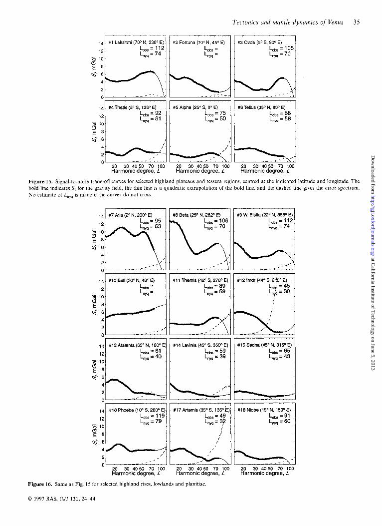
Before considering individual gravity/topography spectra, we note that the gravity field is not equally reliable a t all points on the globe. Considerable variation in field quality exists due to variations in data coverage and spacecraft viewing geometry. We quantify the local resolution of the gravity field by looking at the signal-to-noise behaviour of the gravity field at each location of interest. We obtained estimates of the noise spectra from A. Konopliv (personal communication, 1996) for the 18 selected areas addressed here (Fig. 14). The noise spectra are shown in Figs 15 and 16 together with the S, spectrum for each site. Since we can calculate S, only out to a maximum 1 of 80, we have extrapolated the S, curves with a quadratic extrapolation. The curvature present in many of the SI spectra is the only justification for a quadratic, as opposed to a linear, extrapolation. We use the position-dependent Lobsr defined to be the harmonic degree at which the S , spectrum crosses the error spectrum, to calculate a position-dependent Lny,. In the discussion of the admittance spectra, we clearly indicate where the estimates of L,,, depend on extrapolation of S,, as these are the least reliable. Furthermore, we note that the error spectra have not been calculated using a windowing operation that can be easily related to our localization. Therefore, given these difficulties, we use our estimates of Lnyq (when less than 80) only as guides. Future analyses will need to include a more rigorous treatment of the error structure of the gravity data.

The observed gravity/topography admittance estimates are shown in Figs 17 and 18. For reference, we compare these estimates with those predicted from models which include elastic support, that is models in which the topography is that of a top-loaded plate of elastic thickness T, and crustal thickness D. We apply the model gravity/topography transfer function to the global topography coefficients to predict a set of global gravity coefficients. The two sets of coefficients are subjected to the same spatio-spectral localization as the data in order to generate the reference curves for each location. The reference models are for D = 2 0 and 40km and T,= 10 and 30 km. These curves demonstrate the trade-off between D and z. The difference in the curves as a function of region underscores the need to apply the same localization to both the data and the models. While we could also have included reference curves for models of convection, such dynamic models are non-unique. We note here only that while static compensation models at shallow depths produce relatively flat geoid/topography spectra, dynamic models typically produce red geoid/topography admittance spectra and flat gravity/ topography spectra (e.g. Kiefer et al. 1986; Kiefer & Hager 1991a; McKenzie 1994; Simons 1995).

As found with the geoid/topography admittances, the high-

0 1997 RAS, GJI 131, 24-44



Dow

nloaded from


34 M . Simons, S. C. Solomon and B. H. Huger

1=4

Figure 13. F , with f, = 2. Contours are every 4 m km-'; there are no negative values.

Figure 14. Location map for the individual spectra shown in Figs 15, 16, 17 and 18.

land plateaus (Fig. 17) have much lower gravity/topography admittance values than do the highland rises (Simons et a1 1994). The F , spectra for Lakshmi (#1) and Tellus (#6) are consistent with D z 40 km and T, % 10 km; for Alpha (#5) , D x 20 km and T, x 10 km. For Thetis (#4) and Fortuna (#2), we find Dw20km and T,z20km, although the F , spectra are not well behaved. In all cases, one must keep in mind the size of the feature in question. For instance, the admittance spectrum at Alpha departs at low I from the model prediction at wavelengths much larger than Alpha itself. For Ovda (#3) , F , is more complex than can be accounted for by our simple model. On the basis of these six areas, we conclude that the

F , spectra for the highland plateaus and tesserae are generally consistent with D I 40 km and T, 2 20 km, in agreement with previous analyses (Simons et al. 1994; Grimm 1994). These estimates are also consistent with the estimate for T, of 11-18 km found beneath the Freyja Montes foredeep from a flexural analysis of topographic profiles (Solomon & Head 1990).

The gravity/topography admittances for the highland rises, lowlands and plains (Fig. 18) are, in contrast, not only much larger than for the plateaus and tesserae, but frequently maintain a constant value between 40 and 60 mGal km-' for I 6 40 (Fig. 18). Beyond 1 N 40, the F , spectra frequently exhibit an increase in spectral slope, with a behaviour consistent with elastic support of the topography. Both the admittance magnitude at long wavelengths and the change in spectral character at wavelengths of z 1000 km are consistent with estimates found by McKenzie (1994) for many of the same regions. For most of the regions our estimate of Lnyq corresponds reasonably well with the degree at which the F , spectrum begins trending to zero or where there is increased variation from degree to degree. Imdr Regio (#12) is the best example of close correspondence between L,,,,, and such a change in the F , spectrum. At Bell Regio (#lo) the field is well resolved up to the maximum L,,, of 80, suggesting that the harmonic model has not reached its maximum potential resolution in this region. For Niobe Planitia, the F , spectrum shows no change in behaviour for Lnyq < I < 80, suggesting that we have under- estimated Lnyq, probably because of the quadratic extrapolation of the S, spectrum (Fig. 16). In all cases where

0 1997 RAS, G J I 131, 24-44



Dow

nloaded from


Fig 4

ure 11 <o. c

.. Si (in km) for topography with f ,=2 . All S, maps are shown with red lines for AS,>O, green lines for ASi=O and blue Iontours are every 0.1 m.

0 1997 RAS, GJI 131, 24-44

lines for



Dow

nloaded from


1=4 S,=22.04

Figure 12. AS, (in m) for the geoid with f, = 2. The line convention follows Fig. 11 with contours every 1 m.

0 1997 RAS, G J I 131, 24-44



Dow

nloaded from


Figure 19. Residual geoid after removal of a static model with D = 40 km and T, = 30 km. Contours every 20 m, with geoid height N(R) 2 10 m and I - 10 m shown by red and blue lines, respectively.

0 1997 RAS, GJI 131, 24-44



Dow

nloaded from


Tectonics and mantle dynamics of' Venus 35

14 #1 Lakshrni (70° N, 330° E) #2 Fortuna (70° N, 45O E) #3 Ovda (5O S, 90° E) 1 12 '

m 10. - Lobs = 11 2 Lobs = Lobs = 105,

L = L,, = 70 nyq L", = 74 ' '

20 30 4 0 50 70 100 20 30 .40 50 70 100 20 30 .4050 70 100 Harmonic degree, L Harmonic degree, L Harmonic degree, L

Figure 15. Signal-to-noise trade-off curves for selected highland plateaus and tessera regions, centred at the indicated latitude and longitude. The bold line indicates S, for the gravity field, the thin line is a quadratic extrapolation of the bold line, and the dashed line gives the error spectrum. No estimate of L,,, is made if the curves do not cross.

I I I . ' . " " " I

14. 12,

- m 10 a E

a E 8

#4Thetis ( P S , 125OE) . #5 Alpha (25O S, Oo E) #6 Tellus (35O N, 80° E) Lobs = 92 , , L0,,=75 , , Lobs=88 , L,, = 61 Lnyq = 50 L, = 58

#8 Beta (25O N, 2820 E) Lobs = 106

#I 1 Themis (42O S, 278O E) . L, = 89 L,, = 59

# I 2 lmdr ( 4 4 O S, 2f0° E) Lo&=45 ,

Lnjq = 30 I

#I3 Atalanta (65O N, 160° E . # I4 Lavinia (45O S. 350° E) . Lobs = 59 ,

L, = 39 Lobs = 61 L,, = 40

#I5 Sedna (45O N, 315O E) . Lbs=65 ,

L,, = 43

. #I7 Artemis (35O S, 135Ok) . #I8 Niobe (15" N, 150° E)

Lyq = 60 Lobs= 119, Lobs = 49 , L,,=91 ,

Lnyq = 3? - m 10 I a E

2 n

/

_ - . ., 20 30 ,40 50 70 100 Harmonic degree, L

20 30 4050 70 100 20 30 4050 70 100 Harmonic degree, L Harmonic degree, L

Figure 16. Same as Fig. 15 for selected highland rises, lowlands and planitiae

0 1997 RAS, G J I 131,24-44



Dow

nloaded from


36 M . Simons, S . C. Solomon und B. H. Hager

100 #I Lakshmi (70'N, 330'E)

80

E y 60

E 40 LL"

20

I

- d

n I . . I I I

#4 Thetis (5%, 125'E) #6 Tellus (3.!?N, 80'E)

- 80

5 - 60

E 40 LL--

20

0

I

d

20 30 40 50 6070 20 30 40 50 6070 20 30 40 50 6070 Harmonic Degree, I Harmonic Degree, I Harmonic Degree, I

Figure 17. Gravity/topography admittance spectra for selected highland plateaus and tessera regions, centred at the indicated latitude and longitude. Theoretical curves for compensation at depths of 20 (dashed line) and 40 km (solid line) with effective elastic-plate thicknesses of 10 and 30 km (in order of increasing admittance) are shown for reference. The vertical line indicates the local Nyquist degree; solid black, dashed black and dashed gray lines indicate decreasing levels of confidence.

well-resolved F , spectra follow the predictions for the elastic model a t 12 40, we estimate T, < 30 kin. Again, the trade-off between T, and D is such that compensation for many of these areas could be equally well explained with a slightly smaller value of T, and a slightly larger value of D.

Our best estimates of D and T, values for each region are summarized in Table 1. The characteristic horizontal dimensions listed are very approximate and do not account for the non-circularity of a given feature. In addition, this dimension represents the entire region and not the numerous geological structures within the region.

Table 1. Crustal thickness, D, and effective elastic-plate thickness, T,, for the 18 regions shown in Figs 17 and 18, assuming a crustal density of 2950 kg m-3 and a mantle density of 3250 kg m-3. Characteristic horizontal dimensions are to the nearest 500 km. Ranges for D and T, are given such that the lower (upper) limit for D corresponds to the upper (lower) limit for T,.

# Name Dimension, km D, km T,, km

1 2 3 4 5 6 I 8 9

10 11 12 13 14 15 16 17 18

Lakshmi Planum Fortuna Tessera Ovda Regio Thetis Regio Alpha Regio Tellus Regio Atla Regio Beta Regio W. Eistla Regio Bell Regio Themis Regio Imdr Regio Atalanta Planitia Lavinia Planitia Sedna Planitia Phoebe Regio Artemis Corona Niobe Planitia

2000 2500 2500 2000 1500 1500 2500 2500 2000 1500 2000 1500 3000 2000 2000 2000 2000 3000

40 20 20 20 20 40 40 20-40 -

20-40 20-40 ~

40 -

~

20-40 ~

20-40

10 20 20 20 10 10 30 20-10

30-20 20- 10

30

-

~

-

~

30-20 ~

30

For the highland plateaus and large tessera terrains, the admittances at high harmonic degree are consistent with a single ADC. The ADC value of 40 km for Ishtar Terra (i.e. Lakshmi Planum) implied by our admittances at 12 20 agrees with previous estimates by Simons et al. (1994) and Hansen & Phillips (1995). The ADC values for Western Aphrodite Terra (25-30 km) implied by admittances at 12 30 are sub- stantially lower than previous long-wavelength ADC estimates of 70 and 230 km for western and eastern Aphrodite, respectively (Herrick et al. 1989). For Thetis Regio, Grimm (1994) found evidence for both crustal and dynamic modes of topographic compensation. Our results agree with this conclusion, in that the region of tesserae within Thetis can be modelled as crustally compensated, whereas the remaining portion of Thetis, primarily to the south and including Artemis Chasma, is plausibly dynamically supported. For Atla Regio. our estimate of T, is two-thirds of the 45 f 3 km estimate of Phillips (1994) but the same as the 30 f 5 km estimate of Smrekar (1994). For Bell Regio, our estimate is the same as the 30 5 km short-wavelength estimate of Smrekar (1994). However, the 50 f 5 long-wavelength estimate found in the same study presumably reflects the flattening of the admittance spectrum at longer wavelength, a feature we do not find consistent with elastic support.

The pitfalls of using a spatial GTR estimate are illustrated by the study of Beta Regio by Moore & Schubert (1995), who determined a GTR of 40 m km-' (30 per cent larger than our estimate of 30 m km-' at long wavelengths; see Fig. 13). Moore & Schubert (1995) concluded from a second-order analysis (fitting a parabola instead of a straight line) that the thickness of the thermal lithosphere is approximately 300 km and that models of thermal isostasy (Pratt compensation) require an 800-1000 K temperature anomaly at the base of the lithosphere. From the admittance curve for Beta Regio, we see that a single compensation depth does not fi t &he data. Furthermore, such a large temperature anomaly would be associated with large dynamic stresses, which are ignored in their GTR

0 1997 RAS, G J I 131, 24-44



Dow

nloaded from


Tectonics und mantle dynamics of Venus 3 1

100 I #7 Atla (2'N, 200'E)

7 8ol A 1 #8 Beta (25'N, 282'E) A

106

80

60

E 40 II'

20

- I

m 0

I V" I #I3 Atalanta (65'" 160'E) I

108; I . . . I

r 4

#16 Phoebe (1 O'S, 80

I I I

I

3 - 60

E 40 II'

20

0

8

20 30 40 50 6070 20 30 40 50 6070 Harmonic Degree, I Harmonic Degree, I

Figure 18. Same as Fig. 17 for selected highland rises, lowlands and planitiae.

interpretation. Finally, an 800-1000 K temperature anomaly is excessively large relative to the basalt solidus temperature (e.g. Turcotte & Schubert 1982, p. 144). Similar difficulties arise in the use of the GTR over coronae and rifts (Schubert et al. 1994). Here, as in most GTR studies (e.g. Sandwell & MacKenzie 1989; Kucinskas & Turcotte 1994), the statement is made that the GTR (using the geoid) is, to first order, independent of wavelength in the band 600 km to 4000 km. While this assumption is true for a static compensation model, it is not true for the data. In contrast to the geoid-based GTRs, the gravity/topography admittances frequently appear to be nearly constant at long wavelengths, although the magnitude is much greater than predicted by any reasonable static compensation model.

INTERPRETATION OF THE LOCAL ADMITTANCE

We address the relationship between mantle flow and surface deformation following the reasoning of Simons et al. (1994). Three types of geological provinces are important in this discussion: the highland plateaus and tesserae, the highland

#9 W. Eistla (22N, 358'

20 30 40 50 6070 Harmonic Degree, I

rises, and the plains and lowlands. As described above, the pervasive compressional features and elevated topography of most highland plateaus and tesserae support the hypothesis that the crust in these areas has thickened in response to horizontal shortening. The admittances in these areas are consistent with static compensation of relief by variations in the thickness of a low-density crust. While it has been proposed that these regions represent the surface expression of active crustal shortening and mantle downwelling (Bindschadler & Parmentier 1990 Bindschadler et al. 1990; Zuber 1990; Bindschadler & Head 1991; Kiefer & Hager 1991b; Lenardic, Kaula & Bindschadler 1991; Bindschadler et al. 1992a: Bindschadler, Schubert & Kaula 1992b), the admittance values require no dynamic component of compensation.

In contrast, on the basis of large admittance values and evidence for extensive volcanism, it is generally accepted that the highland rises Beta, Atla, Bell, Eistla, Imdr and Themis Regiones presently overlie sites of mantle upwelling (McGill et al. 1981; Phillips & Malin 1983; Kiefer & Hager 1991a; Smrekar & Phillips 1991; Simons et al. 1994; Smrekar 1994; Stofan et al. 1995; Smrekar & Parmentier 1996). The high topography of the rises results principally from a combination

0 1997 RAS, G J I 131, 24-44



Dow

nloaded from


38 M . Simons, S. C. Solomon and B. H . Huger

of vertical tractions on the base of the lithosphere and crustal thickening by volcanism and magmatic intrusion. The plains and lowlands, like the highland rises, have high admittance values that are not well modelled as static compensation at a single depth. Deformation in these regions subsequent to plains emplacement has been limited and has been concentrated at the ridge belts and wrinkle ridges (Solomon et a/. 1992).

A model in which the crust presently acts only as a passive tracer, such that most long-wavelength topography is the result of the vertical tractions associated with mantle convection, can fit the observed geoid and topography over the rises, plains and lowlands. In this model, highland rises overlie sites of mantle upwelling, and lowlands overlie sites of mantle downwelling. In such a model, the ridge belts in the lowlands are the expression of limited lithospheric strain induced by mantle downwelling (e.g. Zuber & Parmentier 1990). However, a model without substantial crustal deformation cannot explain the large-scale compressional features seen in highland plateaus and the pervasive deformation recorded in the tesserae. Thus, this model can be viable only if such regions formed during a now extinct phase of tectonic deformation (Simons et al. 1994).

The opposing hypothesis states that highland plateaus and tesserae terrains are related to present mantle-flow patterns and that lowlands are regions of incipient or fully developed downgoing mantle flow, which eventually mature to states resembling western Aphrodite Terra or Ishtar Terra (Bindschadler & Parmentier 1990; Bindschadler et a/. 1990; Zuber 1990 Bindschadler & Head 1991; Bindschadler et a/. 1992a,b). Because observed admittances for both lowlands and highlands are positive and bounded, this model is inconsistent with observation (Simons et a/. 1994).

The conclusion that the surface manifestation of convection on Venus has dramatically changed in the past is supported by observations of the density and preservation states of impact craters on the surface of Venus, which indicate an average surface age of about 500 Ma and a low fraction of craters modified by volcanic flows or deformation (Phillips et al. 1991, 1992; Schaber et al. 1992; Strom et al. 1994). Furthermore, the tesserae have a higher density of impact craters larger than 16 km in diameter than d o the plains, and only one-sixth of the large impact craters in the tesserae have been significantly deformed (Ivanov & Basilevsky 1993). Stratigraphic relationships between plains and tessera units consistently indicate that emplacement of plains material occurred after most tessera deformation (Basilevsky & Head 1995). In support of these cratering and stratigraphic observations, new laboratory measurements indicate that the strength of crustal rocks under dry, Venus-like conditions is much greater than previously recognized (Mackwell et al. 1995), implying that the large topographic relief and steep slopes found in the crustal plateaus and mountain belts can be maintained over longer time periods than previously assumed on the basis of the high surface temperature and the estimated strength of crustal rocks on Earth. Consistent with these new measurements of creep strength are Earth-like estimates of T, seen in this study as well as in other studies (e.g. Johnson & Sandwell 1994).

MANTLE VISCOSITY A N D LITHOSPHERE THICKNESS

High values of admittance from earlier global and regional analyses formed the basis for the inferences that Venus lacks an

upper-mantle low-viscosity zone and that convective motions in the mantle couple strongly to the oLerlying lithosphere (Kiefer et al. 1986; Kiefer & Hager 1991a,b; Phillips 1990: Smrekar & Phillips 1991 ). Static compensation models, such as Airy or Pratt models, do not reproduce the observed long- wavelength F , spectra, because they do not account fo r d ) namic stresses induced by mantle flow. Given the inference that the geoid and topography over approximately 90 per cent of Venus are dominated by the effect of vertical convective tractions on the base of the lithosphere, the two fields yield a n approximate map of vertical mantle flow in the Venusian mantle. We would like to use the admittance estimates to constrain the thermal boundary-layer thickness, an important constraint on heat- flow and thermal-evolution models, as well as the a\,erage radial viscosity structure of Venus. In particular. we would like to test for the existence of an Earth-like low-viscosiry zone (LVZ), whether it be a sublithospheric low-viscosity asthenosphere, or a thicker low-viscosity region that spans the full depth extent of the upper mantle (that is above the primary mineralogical phase changes that mark the mantle transition zone on Earth). The issue of a LVZ on Venus has been debated because of its presumed controlling effect on the surface manifestation of convective tractions, either in the form of plate-like behaviour or as large-magnitude horizontal lithospheric strain (e.g. Phillips 1990; Kiefer 1993).

Unfortunately, we can foresee difficulties in our ability to constrain quantitatively the dynamics from geoid and topography data alone. Previous analytic mantle-flow models have shown the non-linear sensitivity of the geoid and topography to the distribution of viscosity and buoyancy forces (e.g. Richards & Hager 1984; Ricard, Fleitout & Froidevaux 1984; Revenaugh & Parsons 1987). Several studies have also applied numerical models of mantle convection to the analysis of gravity and topography on Venus (e.g. Smrekar & Phillips 1991; Kiefer & Hager 1991a, 1992; McKenzie 1994: Moresi & Parsons 1995; Simons 1995; Solomatov & Moresi 1996; Smrekar & Parmentier 1996). The models span a wide range of assumptions regarding the degree of internal heating, the flow geometry (Cartestian or cylindrical axisymmetric), the rheological law (depth-dependent, temperature-dependent, or both) and the effective depth and horizontal extent of the calculation domain. For each study, the success of a given model has usually been determined either by spatial comparisons of observed and model-derived profiles of geoid and topography (for instance, over Beta Regio) or with GTR estimates. On the basis of such measures of fit, all of these models have been reasonably successful, despite the fact that the estimated thickness of the TBL ranged from 70 to 500 km. This variability is the manifestation of the inherent inability to constrain TBL thickness with geoid and topography data.

In areas over which long-wavelength topography and gravity are dominantly the result of convective tractions and thus where T, values probably represent recent thermal conditions, we obtain T, = 10 to 30 km. A similar range was found from topographic profiles outboard of a number of coronae (Johnson & Sandwell 1994). Correcting for the elrects of inelastic yielding (McNutt 1984), Johnson & Sandwell (1994) obtained estimates of the mechanical plate thickness, T,, of about 40 km. For a linear thermal gradient, a temperature of 750°C at a depth T,, a surface at 500°C and a temperature at the base of the TBL of 1250'C, the TBL thickness is then about 120 km. A 120-km TBL thickness is within a factor of

0 1997 RAS. G J I 131, 24-44



Dow

nloaded from



two of that estimated by scaling terrestrial heat flow to Venus (Solomon & Head 1982; Phillips & Malin 1983), under the assumptions that both planets have equal heat production per mass and a similar radial distribution of heat-producing elements, and that heat loss at present occurs solely by steady- state conduction through the lithosphere. Given the estimates of T,, and the realization that single GTR or admittance values d o not constrain TBL thickness, a 45- to 150-km-thick TBL cannot be rejected on the basis of current geophysical understanding. A 300-km-thick TBL is neither required nor favoured by gravity and topography data, estimates of T, or comparisons of convection models with observations.

Analyses discussing the presence of a LVZ on Venus have relied extensively on numerical models scaled to a 600- to 700-km-deep convecting layer with unit aspect ratio flow, corresponding to a maximum wavelength of about 1300 km or 12 30 (e.g. Ceuleneer et al. 1988; Robinson & Parsons 1988; Smrekar & Phillips 1991). These numerical models, originally developed to address the low admittances associated with many oceanic features, can produce arbitrarily low admittances if a LVZ is present (Ceuleneer et al. 1988; Robinson & Parsons 1988). The high values seen at many locations on Venus have therefore been interpreted to be inconsistent with the presence of a LVZ (Phillips 1990; Smrekar & Phillips 1991). However, McKenzie (1994) has shown that if one corrects for constructional volcanism when calculating the observed admittances in the terrestrial ocean basins, then the observed admittances do not show any reduction associated with the presence of the LVZ. Furthermore, on the basis of the Sl maps, the 1300-km length-scales characteristic of the numerical models are much smaller than those associated with the gravity and topography signatures of Atla and Beta. Kiefer & Hager (1991a) conducted numerical experiments scaled for convection in a 2800-km-deep layer and found that an upper mantle extending to 700km depth with a viscosity an order of magnitude less than in the lower mantle could fit the geoid and topography data over Beta and Atla. For their particular model (cylindrical geometry with unit aspect ratio), they found that models with both a low-viscosity upper mantle and an even lower-viscosity asthenosphere underpredicted both the geoid and the topography. In contrast, numerical models conducted in a 2-D polar annulus scaled for whole-mantle convection generated geoid and topography with characteristic amplitudes of 100-200 m and 2-4 km, respectively, and showed no strong modulation by the presence of a low-viscosity region in the upper mantle (Simons 1995). We conclude, therefore, that we do not have sufficient information to determine whether or not there is a LVZ on Venus.

DISCUSSION AND CONCLUSIONS

We have attempted to construct a bridge between the purely spatial and purely spectral approaches to analysing harmonic renditions of globally defined data. This bridge comes in the form of a spatio-spectral localization operator and provides quantitative limits on our ability to determine simultaneously variations in the spatial and spectral domains-limits that are particularly important to determine when manipulating data with finite global spectral resolution.

We have used our localization approach to study the different modes of topographic compensation at length-scales greater than 500 km on Venus, and thereby to constrain the extent to

which convective processes within the planet manifest themselves at the surface. Geoid and topography on Venus are not only positively correlated at all wavelengths when viewed globally, as observed in previous studies, but also when viewed locally. Compensation of relief in the highland plateaus and tesserae, which occupy about 10 per cent of the surface, can be simply explained as the result of Airy isostasy with crustal thicknesses generally not exceeding approximately 40 km. On the basis of impact crater densities and stratigraphic relations, most of the pervasive deformation recorded in the highland plateaus and tesserae must be as old as 500 Ma. More generally, we infer that the present crust of Venus does not thicken or thin significantly in response to convective tractions (Simons et al. 1994).

Local admittances at the shorter wavelengths considered here, as well as in global degree-by-degree analysis (Fig. 3), are consistent with an average planetary crustal thickness of no more than about 30 km. In agreement with this estimate is the continued decrease in elevation commonly seen outboard of the contacts of plains with highland plateaus and tesserae, implying that the crustal thickness beneath these plains is less than beneath these adjacent highlands and tessera blocks. While we cannot exclude the possibility of long-wavelength increases in crustal thickness beneath plains and lowlands distant from highland plateaus and tesserae, such variations must be sufficiently small as not to influence the admittance spectra for plains and lowlands obtained from the presently available gravity field. In contrast to highland plateaus and tesserae, long-

wavelength topographic variations in the rises, plains and lowlands are compensated principally by vertical tractions at the base of the lithosphere. If this model of topographic compensation is correct, then the long-wavelength geoid and topography not associated with the highland plateaus and tesserae yield an approximate map of the vertical convective motions in the upper mantle of Venus (see also Herrick & Phillips 1992). For example, consider the residual geoid shown in Fig. 19, where we have removed a model prediction using D = 40 km and T, = 30 km, which accounts for the component of the geoid that we believe to be statically compensated. This residual geoid is then the minimum field that we associate with convective tractions.

When judging the success of a given compensation model, the peak spatial geoid anomaly should not be the sole criterion, since two different models may yield the same peak anomaly but have very different spectral contents. However, we can ask what portion of the total spatial gravity field is predicted by a given compensation model. From Fig. 19 we see that the static compensation model explains most of the geoid associated with Ovda Regio and the smaller tesserae. Over Ishtar Terra, we reduce the maximum anomaly from over 100m to just over 30 m. Interestingly, there remains a geoid high at Ishtar that is spatially connected to the high associated with Eistla Regio. Hansen & Phillips (1995) also found that two modes of compensation are present a t Ishtar Terra; they favoured a model with a thickened crustal layer overlying a thickened residuum layer, both of which are the result of recent mantle downwelling. From our earlier arguments, however, tesserae and plateaus are probably the fossils remnants of an earlier history of high crustal strain. Within the context of our dynamic compensation model, this viewpoint simply implies mantle upwelling may be occurring beneath Ishtar Terra,

0 1997 RAS, GJI 131, 24-44



Dow

nloaded from


40 M . Simons, S . C. Solomon and B. H. Hager

that is beneath a region that includes a pre-existing highland plateau. Pressure-release partial melting in such an upwelling zone could account for the presence of relatively undisturbed lava plains (Lakshmi Planum) in the centre of an otherwise highly deformed region.

While it is tempting to apply admittance estimates to infer the TBL thickness and mantle viscosity structure of Venus, such efforts are doomed to fail without a prior model of the interior density structure of the planet, because of the inherent non-linearities involved in the forward problem. In contrast to Venus, the structure of the geoid on Earth is complex. Most of the topography is supported by variations in crustal density and thickness, while the long-wavelength geoid is dominated globally by convective processes, with geoid highs associated with both mantle upwellings and mantle downwellings (e.g. Richards & Hager 1988). Dynamic models of the flow- induced geoid resulting from density perturbations derived from seismology or other geophysical inferences (e.g. Hager 1984; Hager et al. 1985) can match the observed geoid and constrain the radial viscosity structure of the Earth, an experi- ment that is not possible to conduct for Venus. We are faced with the conundrum that the relationship between the geoid and the planform of convection appears to be simpler on Venus than on Earth, yet we are able to say more about interior structure for Earth than for Venus because of at least a limited understanding of density anomalies in the Earth’s interior.

The primary differences between the two planets are the lack of active plate tectonics on Venus at present (e.g. Solomon et al. 1992) and the strongly time-dependent history of deformation indicated by the inference from gravity/topography relationships and other considerations that the tesserae and highland plateaus are the surface manifestation of an earlier history of high surface strains. What might account for the profoundly different tectonic styles of Venus and Earth? One hypothesis is that the presence of water may control the surface expression of convection. Since water is a prime factor in weakening lithospheric-scale faults on Earth (e.g. Hickman 1991), the presently anhydrous lithosphere of Venus (e.g. Grinspoon 1993) may prevent the formation of weak plate-boundary faults (McKenzie 1977b; Kaula 1995), thereby inhibiting the development of Earth-like plate tectonics. The need for weak plate margins is illustrated by numerical models of mantle convection that attempt to mimic plate behaviour (that is large- scale horizontal movement with strain concentrated in narrow regions) by incorporating either highly non-linear rheologies or a priori zones of weakness in the lithosphere (e.g. King, Gable & Weinstein 1992; Kiefer 1993; Zhong & Gurnis 1995). If the abundance of water on Venus is related to the surface temperature, then the strong temporal changes in tectonic style on Venus may imply a coupling between atmospheric evolution and the surface manifestation of mantle convection, whereby a more hydrous lithosphere on Venus in the past would have had a lower creep strength (e.g. Mackwell et al. 1995) and may have promoted a more horizontally mobile style of tectonics. Whether such earlier styles could be viewed as products of some form of plate tectonics or another process is presently unknown.

ACKNOWLEDGMENTS

We thank Alex Konopliv and Bill Sjogren for distributing their Venus gravity model before publication. We have benefitted

from discussions with Ming Fang, Tom Jordan, Patrick McGovern, Noriyuki Namiki and Svetlana Panasyuk, as well as from thorough reviews by Catherine Johnson and Roger Phillips. This research was supported by NASA grants NAGW-2161, NAGW-3276, NAGW-3425 and NAG5-4077, and NSF grant EAR-9506427.

REFERENCES

Barsukov, V.L. et al., 1986. The geology and geomorphology of the Venus surface as revealed by the radar images obtained by Veneras 15 and 16, J. geophys. Res., 91, D378-D398.

Basaltic Volcanism Study Project, 1981. Basoific Voicanism on the Terrestrial Planets, Pergamon, New York, NY.

Basilevsky, A.T., 1986. Structure of central and eastern areas of Ishtar Terra and some problems of Venusian tectonics. Geotectonics, 20, 282-288.

Basilevsky, A.T. & Head, J.W., 1995. Global stratigraphy of Venus: Analysis of a random sample of thirty-six test areas, Earth Moon Planets, 66, 285-336.

Bindschadler, D.L. & Head, J.W., 1991. Tessera terrain, Venus: Characterization and models for origin and evolution, J. geophys. Res., 96, 5889-5907.

Bindschadler, D.L. & Parmentier, E.M., 1990. Mantle flow tectonics: The influence of a ductile lower crust and implications for the formation of topographic uplands on Venus, J . geophys. Res., 95, 21 329-21 344.

Bindschadler, D.L., Schubert, G. & Kaula, W.M., 1990. Mantle flow tectonics and the origin of Ishtar Terra, Venus, Geophys. Res. Lett.,

Bindschadler, D.L., deCharon, A,, Beratan, K.K., Smrekar, S.E. & Head, J.W., 1992a. Magellan observations of Alpha Regio: Implications for formation of complex ridged terrains on Venus, J. geophys. Res., 97, 13 563-13 578.

Bindschadler, D.L., Schubert, G. & Kaula, W.M., 1992b. Coldspots and hotspots: Global tectonics and mantle dynamics of Venus, J . geophys. Rex, 97, 13 495-13 522.

17, 1345-1348.

Burchfiel, B.C., 1983. The continental crust, Sci. Am., 249, 130-142. Ceuleneer, G., Rabinowicz, M., Monnereau, M., Cazenave, A. &

Rosemberg, C., 1988. Viscosity and thickness of the sub-lithospheric low-viscosity zone: Constraints from geoid and depth over oceanic swells, Earth planet. Sci. Lett., 89, 84-102.

Chui, C., 1992. An Introduction to Wavelets, Academic Press, San Diego, CA.

Crough, S.T. & Jurdy, D.M., 1980. Subducted lithosphere, hotspots, and the geoid, Earth planet. Sci. Lett., 48, 15-22.

Daubechies, I., 1992. Ten Lectures on Wavelets. Number 61 in CBMS-NSF regional conf. ser. in appl. math, SOC. Indust. Appl. Math., Philadephia, PA.

Edmonds, A.R., 1957. Angular Momentum in Quantum Mechanics, Princeton University Press, Princeton, NJ.

Ford, P.G. & Pettengill, G.H., 1992. Venus topography and kilometre- scale slopes, J. geophys. Res., 97, 13 103-13 114.

Forsyth, D.W., 1985. Subsurface loading and estimates of the flexural rigidity of continental lithosphere, J . geophys. Res., 90, 12 623-13 632.

Grimm, R.E., 1994. The deep structure of Venusian plateau highlands, Icarus, 112, 89-103.

Grimm, R.E. & Phillips, R.J., 1991. Gravity anomalies, compensation mechanisms, and the geodynamics of western Ishtar Terra, Venus, J. geophys. Rex, 96, 8305-8324.

Grimm, R.E. & Phillips, R.J., 1992. Anatomy of a Venusian hot spot: Geology, gravity, and mantle dynamics of Eistla Regio, J . geophys. Rex, 97, 16 035-16 054.

Grinspoon, D.H., 1993. Implications of the high D/H ratio for the source of water in Venus’ atmosphere, Nature, 363, 428-431.

0 1997 RAS, G J I 131, 24-44



Dow

nloaded from



Guest, J.E. et al., 1992. Small volcanic edifices and volcanism in the plains of Venus, J . geophys. Res., 97, 15 949-15 966.

Hager, B.H., 1984. Subducted slabs and the geoid: Constraints on mantle rheology and flow, J. geophys. Res., 89, 6003-6015.

Hager, B.H., Clayton, R.W., Richards, M.A., Comer, R.P. & Dziewonski, A.M., 1985. Lower mantle heterogeneity, dynamic topography and the geoid, Nature, 313, 541-545.

Hansen, V.L. & Phillips, R.J., 1995. Formation of Ishtar-Terra, Venus- Surface and gravity constraints, Geology, 23, 292-296.

Hansen, V.L. & Willis, J.J., 1996. Structural analysis of a sampling of tesserae: Implications for Venus dynamics, kurus, 123, 296-312.

Haxby, W.F. & Turcotte, D.L., 1978. On isostatic geoid anomalies, J . geophys. Res., 83, 5473-5478.

Head, J.W., Campbell, D.R., Elachi, C., Guest, J.E., McKenzie, D.P., Saunders, R.S., Schaber, G.G. & Schubert, G., 1991. Venus volcanism: Initial analysis from Magellan data, Science, 252, 276-288.

Head, J.W., Crumpler, L.S., Aubele, J.C., Guest, J.E. & Saunders, R.S., 1992. Venus volcanism: Classification of volcanic features and structures, associations, and global distribution from Magellan data, J . geophys. Res., 97, 13 153-13 198.

Herrick, R.R. & Phillips, R.J., 1992. Geological correlations with the interior density structure of Venus, J . geophys. Res., 97,

Herrick, R.R., Bills, B.G. & Hall, S.A., 1989. Variations in effective compensation depth across Aphrodite Terra, Venus, Geophys. Res. Lett., 16, 543-546.

Hickman, S.H., 1991. The stress in the lithosphere and the strength of active faults, Rev. Geophys., 29, 759-775.

Ivanov, B.A. & Basilevsky, A.T., 1993. Density and morphology of impact craters on tessera terrain, Venus, Geophys. Res. Lett., 20, 2579-2582.

Janes, D.M. & Squyres, S.W., 1995. Viscoelastic relaxation of topographic highs on Venus to produce coronae, J . geophys. Res., 100,

Johnson, C.L. & Sandwell, D.T., 1994. Lithospheric flexure on Venus, Geophys. J. Int., 119, 627-647.

Jordan, T.H., 1978. Composition and development of the continental tectosphere, Nature, 274, 544-548.

Kaula, W.M., 1966. Global harmonic and statistical analysis of gravimetry, in Geoid Anomalies: Unsurveyed Areas, Vol. 9, pp. 58-67, ed. Orlin, H., Geophys. Mon., Am. Geophys. Un., Washington, DC.

Kaula, W.M., 1967. Theory of statistical analysis of data distributed over a sphere, Rev. Geophys., 5, 83-107.

Kaula, W.M., 1968. An Introduction to Planetary Physics: The Terrestrial Planets, John Wiley, New York, NY.

Kaula, W.M., 1990. Venus: A contrast in evolution to Earth, Science,

Kaula, W.M., 1995. Venus reconsidered, Science, 270, 1460-1464. Kaula, W.M., Bindschadler, D.L., Grimm, R.E., Hansen, V.L.,

Roberts, K.M. & Smrekar, S.E., 1992. Styles of deformation in Ishtar Terra and their implications, J . geophys. Res., 97, 16 085-16 120.

Kiefer, W.S., 1993. Mantle viscosity stratification and flow geometry: Implications for surface motions on Earth and Venus, Geophys. Res. Lett., 20, 265-268.

Kiefer, W.S. & Hager, B.H., 1991a. A mantle plume model for the equatorial highlands of Venus, J . geophys. Res., 96, 20 947-20 966.

Kiefer, W.S. & Hager, B.H., 1991b. Mantle downwelling and crustal convergence: A model for Ishtar Terra, Venus, J . geophys. Res., 96,

Kiefer, W.S. & Hager, B.H., 1992. Geoid anomalies and dynamic topography from convection in cylindrical geometry: Applications to mantle plumes on Earth and Venus, Geophys. J . Int., 108,198-214.

Kiefer, W.S., Richards, M.A., Hager, B.H. & Bills, B.G., 1986. A dynamic model of Venus’s gravity field, Geophys. Res. Lett., 13,

King, S.D., Gable, C.W. & Weinstein, S.A., 1992. Models of convection-

16 017-16 034.

21 173-21 187.

247, 1191-1196.

20 967-20 980.

14-17.

driven tectonic plates: A comparison of methods and results, Geophys. J . Int., 109, 481-487.

Koch, D.M. & Manga, M., 1996. Neutrally buoyant diapirs: A model for Venus coronae, Geophys. Rex Lett., 23, 225-228.

Konopliv, AS. & Sjogren, W.L., 1994. Venus spherical harmonic gravity model to degree and order 60, Icarus, 112, 42-54.

Konopliv, AS. & Sjogren, W.L., 1996. Venus gravity handbook, Technical Report, 96-2, Jet Propulsion Laboratory, California Institute of Technology, Pasadena, CA.

Kucinskas, A.B. & Turcotte, D.L., 1994. Isostatic compensation of equatorial highlands on Venus, kurus, 112, 104-1 16.

Lenardic, A., Kaula, W.M. & Bindschadler, D.L., 1991. The tectonic evolution of Western Ishtar Terra, Venus, Geophys. Rex Lett., 18,

Mackwell, S.J., Zimmerman, M.E., Kohlstedt, D.L. & Scherber, S.S., 1995. Experimental deformation of dry Columbia diabase: Implications for tectonics on Venus, in Proc. 35th U S Symp. Rock Mechanics, pp. 207-214, Reno, NV.

Masursky, H., Eliason, E., Ford, P.G., McGill, G.E., Pettengill, G.H., Schaber, G.G. & Schubert, G., 1980. Pioneer Venus radar results: Geomorphology from images and altimetry, J. geophys. Res., 85,

McGill, G.E., Steenstrup, S.J., Barton, C. & Ford, P.G., 1981. Continental rifting and the origin of Beta Regio, Venus, Geophys. Res. Lett., 8, 737-740.

McKenzie, D.P., 1967. Speculations on the consequences and causes of plate motions, Geophys. J . R. astr. Soc., 18, 1-32.

McKenzie, D.P., 1977a. Surface deformation, gravity anomalies, and convection, Geophys. J . R . astr. Soc., 48, 211-238.

McKenzie, D.P., 1977b. The initiation of trenches: A finite amplitude instability, in Island Arcs, Deep Sea Trenches and Back Arc Basins, Vol. 1, pp. 57-61, eds Talwani, M. & Pitman, W.C., Maurice Ewing Ser., Am. Geophys. Un., Washington, DC.

McKenzie, D.P., 1994. The relationship between topography and gravity on Earth and Venus, Icarus, 112, 55-88.

McNutt, M.K., 1984. Lithospheric flexure and thermal anomalies, J. geophys. Res., 89, 11 180-11 194.

Moore, W.B. & Schubert, G., 1995. Lithospheric thickness and mantle/ lithosphere density contrast beneath Beta Regio, Venus, Geophys. Res. Lett., 22, 429-432.

Moresi, L. & Parsons, B., 1995. Interpreting gravity, geoid, and topography for convection with temperature dependent viscosity: Application to surface features on Venus, J . geophys. Res., 100, 21 155-21 171.

O’Connell, R.J. & Hager, B.H., 1980. On the thermal state of the Earth, in Physics of the Earth’s Interior, Vol. 78, pp. 270-317, eds Dziewonski, A. & Boschi, E., Enrico Fermi intern. School Physics, SOC. ItaIiana di Fisica, Bologna, Italy.

Parmentier, E.M. & Hess, P.C., 1992. Chemical differentiation of a convecting planetary interior: Consequences for a one-plate planet such as Venus, Geophys. Res. Lett., 19, 2015-2018.

Parsons, B. & Richter, F.M., 1980. A relation between the driving force and geoid anomaly associated with mid-ocean ridges, Earth planet. Sci. Lett., 51, 445-450.

Pettengill, G.H., Eliason, E., Ford, P.G., Loriot, G.B., Masursky, H. & McGill, G.E., 1980. Pioneer Venus radar results: Altimetry and surface properties, J . geophys. Res., 85, 8261-8270.

Phillips, R.J., 1990. Convection-driven tectonics on Venus, J. geophys. Res., 95, 1301-1316.

Phillips, R.J., 1994. Estimating lithospheric properties below Atla Regio, Venus, Icarus, 112, 147-170.

Phillips, R.J. & Malin, M.C., 1983. The interior of Venus and tectonic implications, in Venus, pp. 158-214, eds Hunten, D.M., Colin, L., Moroz, V.I. & Donahue, T.M., University of Arizona Press, Tucson, AZ.

Phillips, R.J., Arvidson, R.E., Boyce, J.M., Campbell, D.B., Guest, J.E., Schaber, G.G. & Soderblom, L.A., 1991. Impact craters on Venus: Initial analysis from Magellan, Science, 252, 288-297.

2209-2212.

8232-8260.

0 1997 RAS, G J I 131, 24-44



Dow

nloaded from


42 M . Simons, S . C. Solomon and B. H . Hagrr

Phillips, R.J., Raubertas, R.F., Arvidson, R.E., Sarkar, I.C., Herrick, R.R., Izenberg, N. & Grimm, R.E., 1992. Impact crater distribution on Venus: Implications for planetary resurfacing history, J . geophys. Res., 97, 15 923-15 948.

Price, M. & Suppe, J., 1995. Constraints on the resurfacing history of Venus from the hypsometry and distribution of tectonism, volcanism, and impact craters, Earth Moon Planets, 71, 99-145.

Price, M., Watson, G., Suppe, J. & Brankman, C., 1996. Dating volcanism and rifting on Venus using impact crater densities, J. geophys. Rex , 101, 4657-4671.

Pronin, A.A., 1986. The structure of Lakshmi Planum, an indication of horizontal asthenospheric flow on Venus, Geotectonics, 20,

Pronin, A.A. & Stofan, E.R., 1990. Coronae on Venus: Morphology, classification, and distribution, Icarus, 87, 452-474.

Rappaport, N.R. & Plaut, J.J., 1994. A 360-degree and -order model of Venus topography, Icarus, 112, 27-33.

Revenaugh, J.R. & Parsons, B.P., 1987. Dynamic topography and gravity anomalies for fluid layers whose viscosity varies exponentially with depth, Geophys. J. R . ustr. Soc., 90, 349-368.

Ricard, Y., Fleitout, L. & Froidevaux, C., 1984. Geoid heights and lithospheric stresses for a dynamic Earth, Ann. Geophys., 2, 267-286.

Richards, M.A. & Hager, B.H., 1984. Geoid anomalies in a dynamic Earth, J. geophys. Rex, 89, 5987-6002.

Richards, M.A. & Hager, B.H., 1988. The Earth’s geoid and the large- scale structure of mantle convection, in The Physics of Planets, pp. 247-272, Runcorn, S.K., John Wiley, New York, NY.

Robinson, E.M. & Parsons, B., 1988. Effect of a shallow low-viscosity zone on the formation of midplate swells, J. geophys. Res., 93, 314443156,

Sandwell, D. & MacKenzie, K.R., 1989. Geoid height versus topography for oceanic plateaus and swells, J. geophys. Res., 94,

Sandwell, D.T. & Renkin, M.L., 1988. Compensation of swells and plateaus in the North Pacific: No direct evidence for mantle convection, J . geophys. Res., 93, 2775-2783.

Sandwell, D.T. & Schubert, G., 1992. Flexural ridges, trenches, and outer rises around coronae on Venus, J. geophys. Res., 97,

Saunders, R.S. & Pettengill, G.H., 1991. Magellan: Mission summary, Science, 252, 247-249.

Saunders, R.S., Pettengill, G.H., Arvidson, R.E., Sjogren, W.L., Johnson, W.T.K. & Pieri, L., 1990. The Magellan Venus radar mapping mission, J. geophys. Res., 95, 8339-8355.

Schaber, G.G. et al., 1992. Geology and distribution of impact craters on Venus: What are they telling us?, J. geophys. Rex , 97,

Schroder, P. & Sweldens, W., 1995. Spherical wavelets: Efficiently representing functions on the sphere, in Computer Graphics (SIGGRAPH 95 proceedings), Annual conference series, pp. 161-172, Los Angeies, CA.

Schubert, G., Turcotte, D.L. & Oxburgh, E.R., 1969. Stability of planetary interiors, Geophys. J. R . astr. Soc.. 18, 441-460.

Schubert, G., Moore, W.B. & Sandwell, D.T., 1994. Gravity over coronae and chasmata on Venus, Icarus, 112, 130-146.

Senske, D.A., Schaber, G.G. & Stofan, E.R., 1992. Regional topographic rises on Venus: Geology of western Eistla Regio and comparison to Beta Regio and Atla Regio, J . geophys. Res., 97, 13 395-13 420.

Simons, M., 1995. Localization of gravity and topography: Constraints on the tectonics and mantle dynamics of Earth and Venus, PhD thesis, Massachussetts Institute of Technology, Cambridge, MA.

Simons, M., Hager, B.H. & Solomon, S.C., 1994. Global variations in geoid/topography admittances of Venus, Science, 256, 798-803.

Sjogren, W.L., Bills, B.G., Birkeland, P.W., Esposito, P.B., Konopliv, A.R., Mottinger, N.A., Ritke, S.J. & Phillips, R.J., 1983. Venus gravity anomalies and their correlations with topography, J. geophys. Rex, 88, 1119-1128.

271-281.

7403-7418.

16 069- 16 084.

13 257-13 302.

Sleep, N.H., 1990. Hotspots and mantle plumes: Some phenomenology, J. geophys. Res., 95, 6715-6736.

Sleep, N.H. & Langan, R.T., 1981. Thermal evolution of the Earth: Some recent developments, Adcanres in Geoph~,sic,s, 23, 1 --23.

Smrekar, S.E., 1994. Evidence for active hotspots on Venus from analysis of Magellan gravity data, Icclrus, 112, 2-26.

Smrekar, S.E. & Parmentier, E.M., 1996. The interaction of mantle plumes with surface thermal and chemical boundary layers: Applications to hotspots on Venus, J. geophys. Rex , 101, 5397-5410.

Smrekar, S.E. & Phillips, R.J., 1991. Venusian highlands: Geoid to topography ratios and their implications, Eurth plunet. Sci. Lett.,

Solomatov, V.S. & Moresi, L.N., 1996. Stagnant lid convection on Venus, J . geophys. Res., 101, 4737-4753.

Solomon, S.C., 1993. A tectonic resurfacing model for Venus, Lun. planet. Sci., 24, 1331-1332.

Solomon, S.C. & Head, J.W., 1982. Mechanisms for lithospheric heat transport on Venus: Implications for tectonic style and volcanism, J . geophys. Res., 87, 9236-9246.

Solomon, S.C. & Head, J.W., 1990. Lithospheric flexure beneath the Freyja Montes foredeep, Venus: Constraints on lithospheric thermal gradient and heat flow, Geophys. Res. Lett., 17, 1393-1396.

Solomon, S.C. & Head, J.W., 1991. Fundamental issues in the geology and geophysics of Venus, Science, 252, 252-260.

Solomon, S.C., Head, J.W., Kaula, W.M., McKenzie, D., Parsons, B., Phillips, R.J., Schubert, G. & Talwani, M., 1991. Venus tectonics: Initial analysis from Magellan, Science, 252, 297-31 1.

Solomon, S.C. et al., 1992. Venus tectonics: An overview of Magellan observations, J . geophys. Rex , 97, 13 199-13 256.

Squyres, S.W., Janes, D.M., Baer, G., Bindschadler, D.L., Schubert, G., Sharpton, E.L. & Stofan, E.R., 1992a. The morphology and evolution of coronae on Venus, J. geophys. Res., 97, 13 61 1-13 634.

Squyres, S.W., Jankowski, D.G., Simons, M., Solomon, S.C., Hager, B.H. & McGill, G.E., 1992b. Plains tectonism on Venus: The deformation belts of Lavinia Planitia, J . geophys. Res., 97,

Stofan, E.R., Smrekar, S.E. & Bindschadler, D.L., 1995. Large topographic rises on Venus-Implications for mantle upwelling, J . geophys. Res., 100, 23 317-23 327.

Strom, R.G., Schaber, G.G. & Dawson, D.D., 1994. The global resurfacing of Venus, J. geophys. Rex , 99, 10 899-10 926.

Surkov, Y.A., Moskalyeva, L.P., Shcheglov, O.P., Kharyukova, V.P., Manvelyan, O.S., Kirichenko, V.S. & Dudin, A.D., 1983. Determination of the elemental composition of rocks on Venus by Venera 13 and Venera 14, J . geophys. Res., 88, A481LA493.

Surkov, Y.A., Barsukov, V.L., Moskalyeva, L.P., Kharyukova, V.P. & Kemurdzhian, A.L., 1984. New data on the composition, structure, and properties of Venus rock obtained by Venera 13 and Venera 14, J. geophys. Res., 89, B393-B402.

Surkov, Y.A., Moskalyova, L.P., Kharyukova, V.P., Dudin, A.D., Smirnov, G.G. & Zaitseva, S.Y., 1986. Venus rock composition at the Vega 2 landing site, J. geophys. Res., 91, E215-E218.

Surkov, Y.A., Kirnozov, F.F., Glazov, V.N., Dunchenko, A.G., Tatsy, L.P. & Sobornov, O.P., 1987. Uranium, thorium, and potassium in the Venusian rocks at the landing sites of Vega 1 and 2, J . geophys. Rex, 92, E537-E540.

Turcotte, D.L., 1993. An episodic hypothesis for Venusian tectonics, J . geophys. Res., 98, 17 061-17 068.

Turcotte, D.L. & Schubert, G., 1982. Geodynamics: Applications of Continuum Physics to Geological Problems, John Wiley & Sons, New York, NY.

Varshalovich, D.A., Moskalev, A.N. & Kjersonskii, V.K., 1988. Quantum Theory of Angular Momentum, World Scientific, Singapore.

Walcott, R.I., 1972. Late Quaternary vertical movements in eastern North America: Quantitative evidence of glacio-isostatic rebound, Rev. Geophys. Space Phys., 10, 849-884.

Wilson, J.T., 1965. A new class of faults and their bearing on continental drift, Nature, 207, 343-347.

107, 582-597.

13 579-13 600.

0 1997 RAS, G J I 131, 24-44



Dow

nloaded from



Zhong, S. & Gurnis, M., 1995. Towards a realistic simulation of plate margins in mantle convection, Geophys. Res. Left.. 22, 981- 984.

Zuber, M.T., 1990. Ridge belts: Evidence for regional and local scale deformation on the surface of Venus, Geophys. Res. Lett., 17,

Zuber, M.T. & Parmentier, E.M., 1990. O n the relationship between isostatic elevation and the wavelengths of tectoiiic surface features on Venus, Icarus, 85, 290-308.

1369-1372.

APPENDIX A: THE INVERSE TRANSFORM

A reconstruction algorithm that maps the localized coefficients back to the original field, or, equivalently, to coefficients of the original field, can be accomplished by averaging over all possible positions and rotations of the window. We write the coefficients of the repositioned window as

wfrn(2, P, Y) = C D!n*rn(~, P> l / )w2, > ( A l l m’

where DL,,,,(R) is a Wigner D-function (or a matrix element of the rotation operator) and 0 indicates the original window. We rewrite eq. (21) as

and define the reconstruction as

A(R) = - Y(R, R ) dR , S l Z s, or, using eq. (6),

(‘43)

To show that this reconstruction algorithm is successful, we write eq. (A4) explicitly as

Noting that (Varshalovich et al. 1988)

jR D!,,,,(R) dR = 6f06rno6m~08n2 (‘46)

gives

Eq. (A7) can be further reduced to

1 = ws Yoo(R) > (‘48) which is true by inspection given the definition of wfm and the requirement that W(R) have an average amplitude of 1. For isotropic windows, we can eliminate the c1 rotation, and the reconstruction formula can be simplified to

APPENDIX B: THE COVARIANCE FUNCTION

We develop an expression for the localized cross-covariance function following the formalism of Kaula (1966, 1967) in which a spherical cap window is used. Here we consider the case of an arbitrary window. We introduce a second field B(R) with its corresponding localized field r (R) . Adopting a reference frame centred at R and using A and z to represent, respectively, colatitude and longitude in this reference frame, we define the cross-covariance K(A) as

K ( A ) = A(R)- B(A, Z) d~ dR, j 2’, So2= where the integration over t accounts for all points a fixed distance A away from a given point A@). We write eq. ( B I ) as a degree variance, oiB(/), by expanding K(A) in terms of Legendre polynomials, P I , giving

ciB(1) = 7 1 P,(cos A)K(A) sin A d A , (B2)

where Pf = Pfo. Rewriting this explicitly gives

x lK B(A, t) dr dR sin A dA .

Using the spherical harmonic addition theorem,

and setting R’ = (A, t ) and dR’= dr sin A dA, we write eq. (B3) as

c c

Replacing A(R) and B(R) with their harmonic representations using eq. ( l) , we arrive at the familiar form for the globally averaged degree variance,

&(1) = c a,mb;F,. (B6) m

However, as found by Kaula (1966), replacing A(R) and B(R) with their windowed counterparts, Y(R) and r(fi), results in

o$,(l) = 1 1, j w(n)A(n)Y,*,(n)w(n’)B*(R’)xm(R’) dR dR’.

o$,(l) = c( J WQ)A(Q)Y,*,(R) dR)

m f l

(B7) Rearranging gives

m

x (jn, w(a’)B*(fi’)xm(fi’) do’) 9 (B8)

which, combined with our definition of the localized field from eq. (9), simplifies to

We have shown how to calculate the localized covariance

0 1997 RAS, G J I 131, 24-44



Dow

nloaded from


44 M. Simons, S. C. Solomon and B. H. Hager

for two windowed fields. With a simple rotation, this method can be used to determine the localized covariance, cr~r(Q, /), as a function of l for any point on the sphere. Below, we consider the spherical harmonic expansion of the localized covariance, a}m·(l), which produces a compact representation of the covariance fields in the form of a set of harmonic coefficients for localization at each I. Unlike the global !-dependent estimate of the covariance, rJ80 ( 1)/ fo represents an estimate of the globally averaged covariance that is less spatially biased to regions of locally high variance. This spatial bias has been previously noted in admittance/coherence studies of regions encompassing several geological terranes (Forsyth 1985). While less spatially biased, the spatially averaged localized spectrum is spectrally biased, relative to the periodogram estimate, by the aforementioned convolution operations intrinsic to the transform.

We write the covariance as

(BlO) m

or more explicitly in terms of the original coefficients, we write

ml1 __ .4ml ... 4

(Bll)

For the isotropic window assumed here, after some algebra, eq. (Bll) may be rewritten as

X(~ lz I)C3 14 l) c2 !4 l') 0 0 0 0 0 0 0 0

X cl lz I)C3 14 l) ( 12 [4 [') ml mz m m3 m4 m -m2 1114 m'

(Bl2)

As was seen with the windowed field estimate, the covariance estimate at degree l is sensitive to data with degree less than l + Lwin (equal to 1.51 when using J, = 2). Similarly, from the third 3-j coefficient in eq. (Bl2), we find that the covariance expansion at degree l has a maximum degree of 2Lwin (equal to l when using j, = 2), providing a measure of the minimum length-scale over which the covariance function will vary. Note that this scale is a function only of the maximum degree of the window expansion. If the window were a constant over the whole sphere, then it would have only the single I'= 0, m' = 0 term and, as expected, the covariance would not vary over the sphere.

The above derivation is useful for understanding the structure of the covariance estimates. However, for computational purposes we invoke the definition of the localized field from eq. (B9) to calculate the localized coefficients for a given geographic location, and we use these coefficients to calculate the covariances at that point. This procedure is repeated for the set of desired points (for example a grid or a great circle).

© 1997 RAS, GJI 131, 24-44



Dow

nloaded from


Localization of gravity and topography: constraints on the … · 2017-02-27 · both the geoid and...

Documents

Transcript of Localization of gravity and topography: constraints on the … · 2017-02-27 · both the geoid and...