1

Localization Methods for a Mobile Robot in Urban

EnvironmentsAtanas Georgiev, Member, IEEE, and Peter K. Allen, Member, IEEE

Abstract— This paper addresses the problems of building afunctional mobile robot for urban site navigation and modelingwith focus on keeping track of the robot location. We havedeveloped a localization system that employs two methods. Thefirst method uses odometry, a compass and tilt sensor, and aglobal positioning sensor. An extended Kalman filter integratesthe sensor data and keeps track of the uncertainty associated withit. The second method is based on camera pose estimation. It isused when the uncertainty from the first method becomes verylarge. The pose estimation is done by matching linear featuresin the image with a simple and compact environmental model.We have demonstrated the functionality of the robot and thelocalization methods with real-world experiments.

Index Terms— Mobile robots, localization, machine vision

I. INTRODUCTION

THE problem of building a functional autonomous mobile

robot that can successfully and reliably interact with the

real-world is very difficult. It involves a number of issues

— such as proper design, choice of sensors, methods for

localization, navigation, planning, and others, — each of which

is a challenge on its own. A key factor of this complexity is

the targeted environment of operation. The current state of

mobile robotics is that most of the research has been focused

on solving these issues indoors because of the slightly more

predictable nature (e.g. flat horizontal floors, well-structured

space partitioning, smaller scale, etc). On the other hand,

many of the interesting applications are outdoors where fewer

assumptions can be taken for granted.

In this paper, we target outdoor urban environments. These

environments pose their own unique set of challenges that

differentiate them from both the indoor and the open-space

outdoor landscapes. On the one hand, they are usually too large

to consider applying certain techniques that achieved success

indoors. On the other hand, typical outdoor sensors, such as

GPS, have problems with reception around buildings.

While we have tried to keep the methods presented here

general, we have focused on the development of our mobile

robot system (Figure 1) with a specific application in mind.

The AVENUE project at the Columbia University Robotics

Laboratory targets the automation of the urban site modeling

process [1]. The main goal is to build geometrically accurate

and photometrically correct models of complex outdoor urban

environments. These environments are typified by large 3-D

structures that encompass a wide range of geometric shapes

and a very large scope of photometric properties.

High-quality site models are needed in a variety of appli-

cations, such as city planning, urban design, fire and police

planning, historical preservation and archaeology, virtual and

Scanner

Network

Camera

PTU

Sonars

GPS

DGPS

PC

Compass

Fig. 1. The mobile platform used in this work.

augmented reality, geographic information systems and many

others. However, they are typically created by hand which is

extremely slow and error prone. The models built are often

incomplete and updating them can be a serious problem.

AVENUE addresses these issues by building a mobile system

that will autonomously navigate around a site and create a

model with minimum human interaction if any.

The design and implementation of our mobile platform

involved efforts that are related and draw from a large amount

of existing work. For localization, dead reckoning has always

been attractive because of its pervasiveness [2]–[4]. With the

rapid development of technology, GPS receivers are quickly

becoming the sensor of choice for outdoor localization [5]–

[7]. Imaging sensors, such as CCD cameras and laser range

finders, have also become very popular mobile robot com-

ponents [8]–[11]. Various methods for sensor integration and

2

GPS PTURobotCompassCameraScanner

Odo Drive PTU

Controller

Navigator

Localizer

AttitudeGPSImageScan

videoserver

GPSserver

attitudeserver

ATRV-2server

PTUserver

navserver

scanserver

Modeler ViewPlanner PathPlanner

UserInterfaceImages,

ModelsAreaMaps

on-boardPC

remotehost 1

remotehost 3

remotehost 2

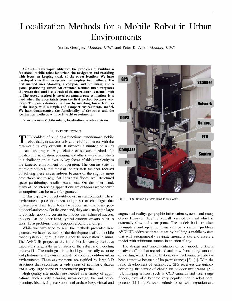
Fig. 2. The system architecture. Solid rectangles represent components, dotted rectangles are processes, and dashed rectangles group processes running onthe same machine. The arrows show the data flow between components.

uncertainty handling have been proposed [12]–[16]. A very

popular and successful idea is to exploit the duality between

localization and modeling and address both issues in the same

process, known as SLAM – Simultaneous Localization and

Map Building [14], [15], [17], [18]. Sensors and methods for

indoor localization have been comprehensively reviewed in

two books [19], [20]. Another excellent book presents case

studies of successful mobile robot systems [21].

Researchers from the Australian Centre for Field Robotics

have made significant progress toward using SLAM in outdoor

settings. Dissanayake et al have proved that a solution to the

SLAM problem is possible and presented one such implemen-

tation [22]. Guivant et al have further looked into optimizing

the computational aspects of their algorithm and have applied

it to an unstructured natural environment [23].

The problem of mobile robot localization in urban environ-

ments has been addressed by Talluri and Aggarwal by using

feature correspondences between images taken by a camera on

the robot and a CAD or similar model of its environment [24].

Chen and Shibasaki have improved on the accuracy and

stability of GPS in urban areas by adding a camera and a

gyro [25]. They have also relied on an environmental model

obtained from a geodetic information system. Nayak has used

a sensor suite consisting of four GPS antennae and a low-

cost inertial measurement unit for localization of a car in

urban areas, however, their resulting localization errors were

on the order of meters which is not acceptable for mobile robot

navigation [26].

Our approach delivers a mobile robot system capable of

operating autonomously under the challenges of urban envi-

ronments. Whenever needed, we are making use of unique

urban characteristics to facilitate the estimation of the robot

location. Of all outdoor environments, urban areas seem to

possess the most structure in the form of buildings. The

laws of physics dictate common architectural design principles

according to which the horizontal and vertical directions play

an essential role and parallel line features are abundant. The

system presented here takes advantage of these characteristics.

We believe that the main contributions of our work are the

practical realization of a functioning mobile robot for site

navigation and modeling and a novel method of supplementing

odometry and GPS with visual image processing to allow

accurate localization of the robot under varying conditions

including odometry error and GPS degradation.

The rest of this paper is organized as follows: The next

section briefly describes our mobile system and software archi-

tecture. Section III describes the first of our localization meth-

ods, based on odometry, a digital compass module and global

positioning. Section IV presents our vision-based localization

methods. Experimental results are shown in section V and in

section VI, we conclude with a summary and a discussion on

future extensions of this work.

II. SYSTEM DESIGN AND IMPLEMENTATION

The mobile robot used as a test bed for this work is an

ATRV-2 model manufactured by iRobot (Figure 1). It has

built-in odometry, twelve sonars and carries a regular PC on-

board. For modeling, we have installed a Cyrax 2500 laser

range scanner with a range of up to 100m. For navigation,

we have added a Honeywell HMR3000 digital compass mod-

ule with an integrated roll-pitch sensor, an Ashtech GG24C

3

Fig. 3. The user interface. The window shows the outlines of the 2-D mapand simplified 3-D models of buildings. The actual trajectories of two robotsare visible along with the planned path for the red robot (denoted with flags).

GPS+GLONASS1 receiver which is accurate down to 1 cm in

real-time kinematic (RTK) mode, and a color CCD camera

mounted on a pan-tilt unit (PTU). Communication with the

robot is done via a 802.11b wireless network.

The combination of dead-reckoning and GPS is known to

be beneficial. GPS tends to exhibit an unstable high-frequency

behavior manifested by sudden “jumps” of the position esti-

mates but is fairly reliable over a longer period of time. On the

other hand, dead-reckoning sensors drift gradually and rarely

suffer the sudden jump problem.

The camera is needed to address some of the limitations of

GPS operation that are quite consistent in urban areas. Tall

buildings in the vicinity may obstruct the clear view to the

satellites, the signal-to-noise ratio could be attenuated by trees

or large structures standing in the way or one may encounter

signal reflections or multipath. The result is unstable, wrong,

or even no position fixes in some areas. However, due to the

nature of urban sites and the overall goal of AVENUE, it is

mostly around buildings that degradation in GPS performance

is likely to occur. With the addition of a camera, we make

use of this by exploiting typical urban characteristics, such as

abundance of linear features, parallel lines, and horizontal and

vertical principal directions, which are relatively easy to find

and process using computer vision techniques.

Our system architecture (Figure 2) addresses the various

tasks associated with an autonomous navigation and modeling

in a modular and distributed fashion. Its main building blocks

are concurrently executing distributed software components

which can communicate across the network. The robot is

designed to operate according to the following scenario: Its

1Throughout this paper we will use GPS to designate any or both of theU.S. NAVSTAR GPS and the Russian GLONASS infrastructures.

Odometry

Compass

GPS

true orientation+compass errors

true pose odometry errors

true position+GPS errors

+

+odometry errors+

compass/GPS errors

corrected odometry pose

odometry error estimates

zk

zk

h(x)~

h(x)~Kalman

Filterzk

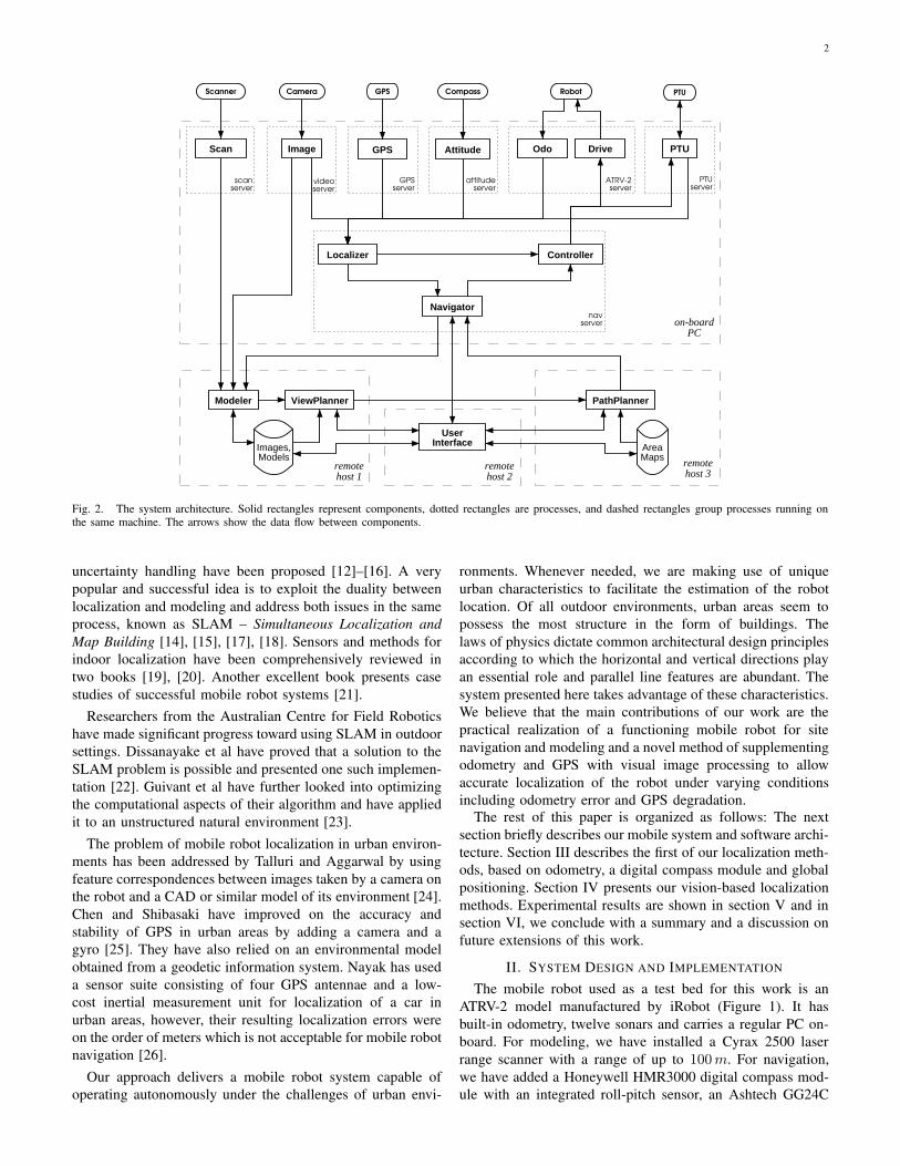
Fig. 4. A diagram of the extended Kalman filter configuration.

task is to go to desired locations and acquire requested 3-

D scans and images of selected buildings. The locations are

determined by the sensor planning system and are used by the

path planning system to generate reliable trajectories which the

robot follows. When the rover arrives at the target location, it

uses the sensors to acquire the scans and images and forwards

them to the modeling system. The modeling system registers

and incorporates the new data into the existing partial model

of the site (which in the beginning could be empty). After

that, the view planning system decides upon the next best data

acquisition location and the above steps repeat. The process

starts from a certain location and gradually expands the area

it has covered until a complete model of the site is obtained.

The user interface (Figure 3) provides a comprehensive view

of the robot location and activities within its environment and

allows the user to monitor the progress and exercise control

of the mission.

The entire task is quite complex and requires the solution of

a number of additional fundamental problems which we have

addressed in our project. Due to limited space, we refer the

reader to [27]–[29].

III. LOCALIZATION IN OPEN SPACE

The first of our localization methods is designed for real-

time usage in open-space outdoor environments. It uses the

built-in robot odometry and the added digital compass/tilt

sensor and GPS receiver. We exploit the redundancy in the

measurements of these sensors to fuse their estimates using

an extended Kalman filter shown in Figure 4 [30].

The control input to the robot consists of the scalar transla-

tional velocity v(t) and the scalar angular velocity ω(t). Due

x

y xy

∆φ

∆s

Fig. 5. The ATRV kinematics.

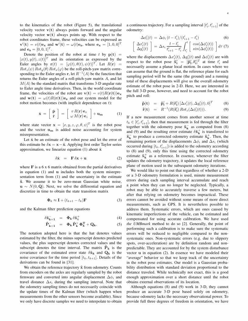
4

to the kinematics of the robot (Figure 5), the translational

velocity vector v(t) always points forward and the angular

velocity vector w(t) always points up. With respect to the

robot coordinates frame, these velocities can be expressed as

v′(t) = v(t)ex and w′(t) = ω(t)ez, where ex = [1, 0, 0]T

and ez = [0, 0, 1]T .

Denote the position of the robot at time t by p(t) =[x(t), y(t), z(t)]T and its orientation as expressed by the

Euler angles by r(t) = [ϕ(t), θ(t), ψ(t)]T . Let R(r) =Rotz(ψ)Roty(θ)Rotx(ϕ) be the roll-pitch-yaw matrix corre-

sponding to the Euler angles r, let R−1(A) be the function that

returns the Euler angles of a roll-pitch-yaw matrix A, and let

M(A) be the standard matrix that transforms 3-D angular rate

to Euler angle time derivatives. Then, in the world coordinate

frame, the velocities of the robot are v(t) = v(t)R(r(t))ex

and w(t) = ω(t)R(r(t))ez and our system model for the

robot motion becomes (with implicit dependence on t):

x =

[

p

r

]

=

[

v R(r) ex

ωM(r) ez

]

+ um (1)

where state vector x = [x, y, z, ϕ, θ, ψ]T is the robot pose

and the vector um is added noise accounting for system

misrepresentation.

Let x be an estimate of the robot pose and let the error of

this estimate be δx = x− x. Applying first order Taylor series

approximation, we linearize equation (1) about x

δx = F δx + u (2)

where F is a 6 x 6 matrix obtained from the partial derivatives

in equation (1) and u includes both the system misrepre-

sentation term from (1) and the uncertainty in the estimate

x. We assume it to be zero-mean Gaussian white noise,

u ∼ N(0,Q). Next, we solve the differential equation and

discretize in time to obtain the state transition matrix

Φk ≈ I + (tk+1 − tk)F (3)

and the Kalman filter prediction equations

δx−

k+1 = Φk δx+

k (4)

P−

k+1 = Φk P+

k ΦTk + Qk. (5)

The notation adopted here is that the hat denotes values

estimated by the filter, the minus superscript denotes predicted

values, the plus superscript denotes corrected values and the

subscript denotes the time interval. The matrix Pk is the

covariance of the estimated error state δxk and Qk is the

noise covariance for the time period [tk, tk+1]. Details of the

derivations can be found in [31].

We obtain the reference trajectory x from odometry. Counts

from encoders on the axles are regularly sampled by the robot

firmware and converted into angular displacement ∆φi and

travel distance ∆si during the sampling interval. Note that

the odometry sampling times do not necessarily coincide with

the update times of the Kalman filter (which happen when

measurements from the other sensors become available). Since

we only have discrete samples we need to interpolate to obtain

a continuous trajectory. For a sampling interval [t′i, t′

i+1] of the

odometry:

∆φ′i(t) = ∆φi (t− t′i)/(t′

i+1 − t′i) (6)[

∆x′i(t)∆y′i(t)

]

= ∆si

t− t′it′i+1

− t′i

∫ t

t′i

[

cos(∆φ′i(t))sin(∆φ′i(t))

]

dτ (7)

where the displacements ∆x′i(t), ∆y′i(t) and ∆φ′i(t) are with

respect to the robot pose x′

i = [p′

i, r′

i]T at time t′i and

necessarily assume a planar local motion. In cases where we

can assume that the ground is flat, the reference plane for each

sampling period will be the same (the ground) and a running

total of these displacements will give us the overall odometry

estimate of the robot pose in 2-D. Here, we are interested in

the full 3-D pose, however, and need to account for the robot

pitch and roll:

p(t) = p′

i +R(r′i) [∆x′i(t),∆y′

i(t), 0]T (8)

r(t) = R−1(R(r′i)Rotz(∆φ′

i(t))). (9)

If a new measurement comes from another sensor at time

tk ∈ [t′i, t′

i+1], then that measurement is fed through the filter

together with the odometry pose x−

k as computed from (8)

and (9) and the resulting error estimate δx+

k is transferred to

x−

k to produce a corrected odometry estimate x+

k . Then, the

remaining portion of the displacements ∆φi and ∆si (which

occurred during [tk, t′

i+1]) is added to the odometry according

to (8) and (9), only this time using the corrected odometry

estimate x+

k as a reference. In essence, whenever the filter

updates the odometry trajectory, it updates the local reference

plane of motion used in the subsequent odometry iterations.

We would like to point out that regardless of whether a 2-D

or a 3-D odometry formulation is used, minute measurement

errors during each sampling interval accumulate and reach

a point when they can no longer be neglected. Typically, a

robot may be able to accurately traverse a few meters, but

after that relying on odometry becomes impractical. These

errors cannot be avoided without some means of more direct

measurements, such as GPS. It is nevertheless possible to

address them. Systematic errors, which are ones caused by

kinematic imperfections of the vehicle, can be estimated and

compensated for using accurate calibration. We have used

the UMBmark method to do so [2]. Generally, the point of

performing such a calibration is to make sure the systematic

errors will be reduced to negligible compared to the non-

systematic ones. Non-systematic errors (e.g. due to slippery

spots, over-acceleration) are by definition random and non-

predictable. They are accounted for by the system disturbance

vector u in equation (2). In essence we have modeled their

“average” behavior so that we keep track of the uncertainty

in the robot pose estimates. Our model is a Gaussian proba-

bility distribution with standard deviation proportional to the

distance traveled. While technically not exact, this is a good

enough approximation over a short distance until the robot

obtains external observations of its location.

Although equations (8) and (9) work in 3-D, they cannot

produce an accurate 3-D pose based solely on odometry,

because odometry lacks the necessary observational power. To

provide full three degrees of freedom in orientation, we have

5

added a compass and tilt sensor module which reports the

heading (yaw), pitch and roll angles. It is mounted level on the

robot and is calibrated for magnetic variation and deviation.

The observation model is quite simple as it is already linear:

zck = [ϕc

k, θck, ψ

ck]T (10)

Hck =

0 0 0 1 0 00 0 0 0 −1 00 0 0 0 0 −1

(11)

Rck = diag(σ2

t , σ2t , σ

2h) (12)

where zck is the sensor measurement vector, Hc

k is the observa-

tion matrix and Rck is the observation uncertainty. The negative

signs in Hck are due to the sensor coordinate system being

oriented forward-right-down while the robot frame is forward-

left-up. We assume a Gaussian distribution of the measurement

error with tilt and heading standard deviations, σt and σh,

based on the manufacturer’s specifications. The sensor data

is used to update the state vector according to the standard

Kalman filter equations:

Kk+1 = P−

k+1 HTk+1 (Hk+1 P−

k+1 HTk+1 + Rk+1)−1(13)

δzk+1 = zk+1 −Hk+1 x−

k+1 (14)

δx+

k+1 = δx−

k+1 + Kk+1 [δzk+1 −Hk+1 δx−

k+1] (15)

P+

k+1 = (I −Kk+1 Hk+1) P−

k+1. (16)

The GPS receiver is very useful because it limits the error ac-

cumulated by the dead reckoning sensors. It provides periodic

fixes of the location of the GPS antenna, zgk = [xg

k, ygk, z

gk ]T .

Since the antenna is placed at location ∆pg with respect to the

robot coordinate frame, the observation model is not linear:

hg(x) = p +R(r)∆pg. (17)

The fix is incorporated into the filter via equations (13)–

(16) where the observation matrix is Hgk = ∇hg(x)|x−

k

and

the measurement uncertainty Rgk is the one reported by the

receiver.

The GPS is the only sensor in this method that makes

absolute position measurements and thus the overall accuracy

of the method depends strongly on the accuracy of the GPS

fixes. If GPS quality deteriorates, the uncertainty in the pose

estimates may become too large. In such cases, positioning

data is needed from additional sensors. But in order to seek

such data, there has to be a way to detect these situations.

This is done by monitoring the variance-covariance matrix

representing the uncertainty in the Kalman filter. Each of the

diagonal elements of this matrix reflects the variance of the

corresponding element (position or orientation coordinate) of

the state vector. Whenever a new GPS update is processed by

the filter, a test is performed to check if the variance associated

with the robot position is greater than a threshold. If so, we

consider this as an indication that additional data is needed

and attempt to use the visual localization method described

next. Only the uncertainly in position is considered because

if the orientation is wrong it will quickly cause the position

error to also increase.

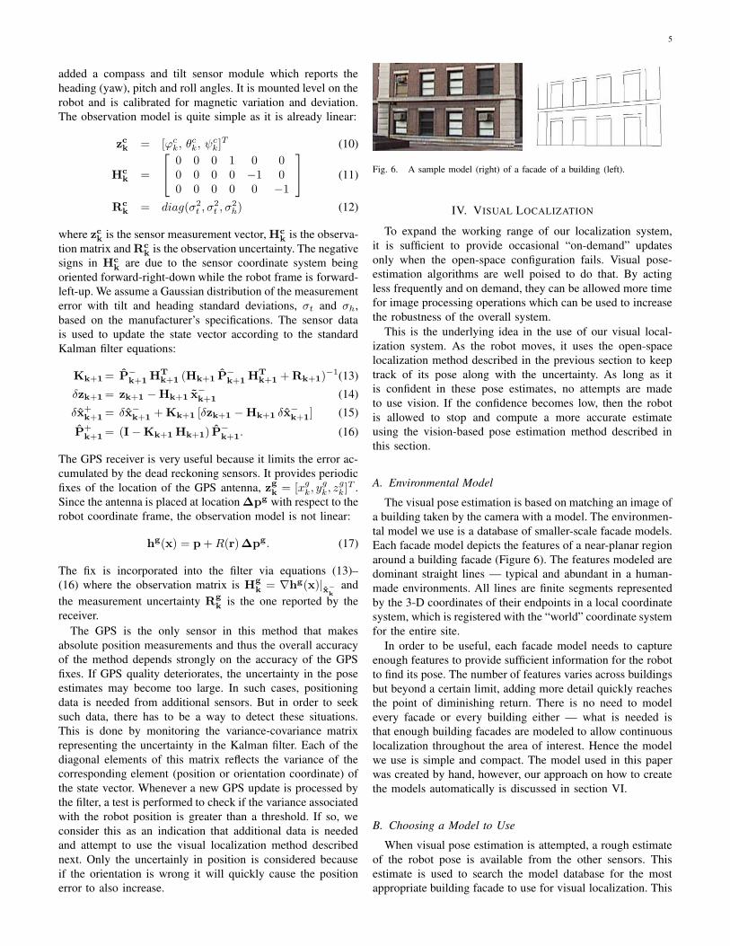
Fig. 6. A sample model (right) of a facade of a building (left).

IV. VISUAL LOCALIZATION

To expand the working range of our localization system,

it is sufficient to provide occasional “on-demand” updates

only when the open-space configuration fails. Visual pose-

estimation algorithms are well poised to do that. By acting

less frequently and on demand, they can be allowed more time

for image processing operations which can be used to increase

the robustness of the overall system.

This is the underlying idea in the use of our visual local-

ization system. As the robot moves, it uses the open-space

localization method described in the previous section to keep

track of its pose along with the uncertainty. As long as it

is confident in these pose estimates, no attempts are made

to use vision. If the confidence becomes low, then the robot

is allowed to stop and compute a more accurate estimate

using the vision-based pose estimation method described in

this section.

A. Environmental Model

The visual pose estimation is based on matching an image of

a building taken by the camera with a model. The environmen-

tal model we use is a database of smaller-scale facade models.

Each facade model depicts the features of a near-planar region

around a building facade (Figure 6). The features modeled are

dominant straight lines — typical and abundant in a human-

made environments. All lines are finite segments represented

by the 3-D coordinates of their endpoints in a local coordinate

system, which is registered with the “world” coordinate system

for the entire site.

In order to be useful, each facade model needs to capture

enough features to provide sufficient information for the robot

to find its pose. The number of features varies across buildings

but beyond a certain limit, adding more detail quickly reaches

the point of diminishing return. There is no need to model

every facade or every building either — what is needed is

that enough building facades are modeled to allow continuous

localization throughout the area of interest. Hence the model

we use is simple and compact. The model used in this paper

was created by hand, however, our approach on how to create

the models automatically is discussed in section VI.

B. Choosing a Model to Use

When visual pose estimation is attempted, a rough estimate

of the robot pose is available from the other sensors. This

estimate is used to search the model database for the most

appropriate building facade to use for visual localization. This

6

Fig. 7. Choosing a model: A top-down view of modeled facades of buildingsare shown on the map. The two circles show the minimum and maximumdistance allowed. The dotted lines are models that are outside of this range.The dashed lines are models that are within the range but are viewed at avery low (or negative) angle. The solid lines are good to use. The thick oneis chosen because it is closest to the robot.

is done in two steps according to two criteria: distance and

viewing angle (Figure 7).

The first step is to scan through the model database index to

determine the facade models that are within a good distance

from the robot. Both minimal and maximal limits are imposed:

If a building is too close, it may not have enough visible

features on the image; if it is too far, the accuracy of the

result may be low because of the fixed camera resolution.

The second step is to eliminate facade models from the

first step based on the viewing angle (ranging from 90◦ for

an anterior view to −90◦ for a posterior view). Only models

that are viewable under a large enough angle are considered.

This eliminates both the facades that are not visible (negative

angles) and the ones that are visible at too low an angle to

produce a stable match with the image.

The models that successfully pass this two-step selection

process form the set of good candidate models to use. Any

subset of this set can be used in the pose estimation step. As

the processing time is not trivial, however, we choose to use

only the one that is closest to the robot. Because of the finite

resolution of the camera, this choice is likely to provide the

most accurate result.

Finally, the pan-tilt head holding the camera is turned

toward the chosen facade and an image is taken. The pan and

tilt angles are computed from the known rough pose of the

robot so that the camera faces the center of mass of the model.

In practice, the final orientation of the camera is different

from the ideal one because of the uncertainty in the current

pose. However, for the small distances involved and the typical

accuracy of the pose estimates, the resulting orientation error

of the camera is usually within the tolerance of the processing

steps that follow. Further, since the camera is aimed at the

center of the model, any small deviation will have minimal

effect.

C. Pose Estimation

At this stage, a pair of an image and a model of the building

facade are available and the task is to determine the pose of the

N

sj

ej,1ej,2

Pj,1

Pj,2

cameracenter

world coordinatesystem

2D edge onthe image

3D line feature

R, T

distances from3D line endpointsto plane formed

by edge line

l i

i

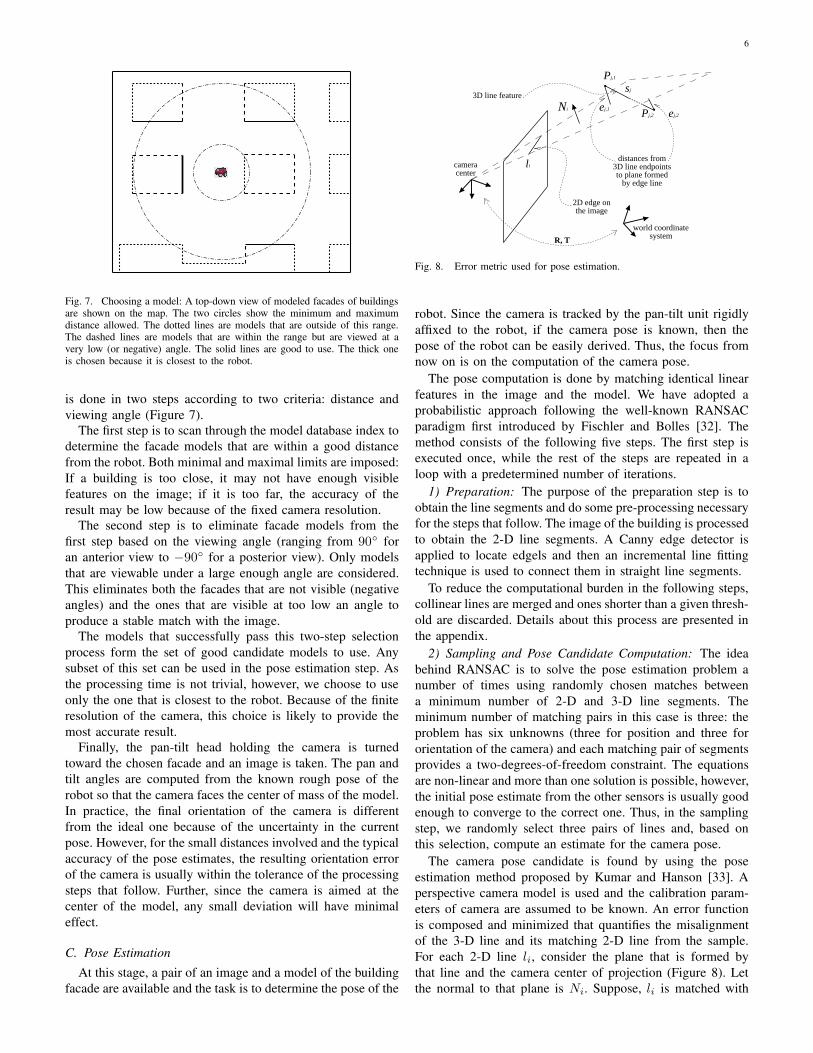
Fig. 8. Error metric used for pose estimation.

robot. Since the camera is tracked by the pan-tilt unit rigidly

affixed to the robot, if the camera pose is known, then the

pose of the robot can be easily derived. Thus, the focus from

now on is on the computation of the camera pose.

The pose computation is done by matching identical linear

features in the image and the model. We have adopted a

probabilistic approach following the well-known RANSAC

paradigm first introduced by Fischler and Bolles [32]. The

method consists of the following five steps. The first step is

executed once, while the rest of the steps are repeated in a

loop with a predetermined number of iterations.

1) Preparation: The purpose of the preparation step is to

obtain the line segments and do some pre-processing necessary

for the steps that follow. The image of the building is processed

to obtain the 2-D line segments. A Canny edge detector is

applied to locate edgels and then an incremental line fitting

technique is used to connect them in straight line segments.

To reduce the computational burden in the following steps,

collinear lines are merged and ones shorter than a given thresh-

old are discarded. Details about this process are presented in

the appendix.

2) Sampling and Pose Candidate Computation: The idea

behind RANSAC is to solve the pose estimation problem a

number of times using randomly chosen matches between

a minimum number of 2-D and 3-D line segments. The

minimum number of matching pairs in this case is three: the

problem has six unknowns (three for position and three for

orientation of the camera) and each matching pair of segments

provides a two-degrees-of-freedom constraint. The equations

are non-linear and more than one solution is possible, however,

the initial pose estimate from the other sensors is usually good

enough to converge to the correct one. Thus, in the sampling

step, we randomly select three pairs of lines and, based on

this selection, compute an estimate for the camera pose.

The camera pose candidate is found by using the pose

estimation method proposed by Kumar and Hanson [33]. A

perspective camera model is used and the calibration param-

eters of camera are assumed to be known. An error function

is composed and minimized that quantifies the misalignment

of the 3-D line and its matching 2-D line from the sample.

For each 2-D line li, consider the plane that is formed by

that line and the camera center of projection (Figure 8). Let

the normal to that plane is Ni. Suppose, li is matched with

7

the 3-D line segment sj whose endpoints Pj,1 and Pj,2 have

world coordinates pj,1 and pj,2. If R and T are the rotation

and translation that align the world coordinate system with the

one of the camera, then

di,j = (Ni · (R · pj,1 + T ))2 + (Ni · (R · pj,2 + T ))2 (18)

is the sum of squared distances of the endpoints of sj to

the plane formed by li (Figure 8). The error function that

is minimized is the sum of di,j for the three matching pairs:

E(R, T ) =∑

i,j∈Matches

di,j . (19)

This function is minimized with respect to the six degrees

of freedom for the camera pose: three for the rotation R and

three for the translation vector T . The computation follows

the method proposed by Horn [34].

3) Pose Candidate Refinement: The pose candidate refine-

ment step uses the consensus set to fine tune the estimate.

The consensus set is the set of all matching pairs of 2-D

edge segments from the image and 3-D line segments from the

model that agree with the initially computed pose candidate.

For each 3-D line segment in the model, a neighborhood of

its projection on the image is searched for 2-D edges and their

distance from the 3-D line segment is computed according to

(18). The 2-D edge with the smallest distance is taken to be

the match, if that distance is less than a threshold and if the

2-D line is not closer to another 3-D line. If no such 2-D edge

is found, then the 3-D line segment is assumed to have no

match.

The consensus set is used together with equation (19) to

compute a better pose estimate. This is done iteratively a

number of times (between 1 and 4) starting with a large value

for the consensus threshold and gradually decreasing it. The

large initial value for the threshold makes sure that a roughly

correct consensus set will be generated initially which will be

later refined to eliminate the false positives and increase the

accuracy. The result of the last iteration is the pose candidate

that is evaluated in the next step.

4) Pose Candidate Evaluation: The quality of each pose

candidate is judged by a metric q(R, T ) which quantifies the

amount of support for the pose by the matches between the

model and the edge. The idea is to check what portion of

the model is covered by matching edge lines. The larger the

coverage, the better the pose candidate. Ideally, the entire

visible portion of the model should be covered by matching

2-D edge lines.

After the last refinement iteration, the consensus set contains

pairs of matching 3-D lines from the model and 2-D lines from

the edges. Consider one 3-D line sj in the consensus set and

its matching 2-D counterpart li. Let the perspective projection

of sj onto the image be s′j and the orthogonal projection of

li onto s′j be l′i. We set the contribution c(sj) of the match

between sj and li to the length of the overlap between s′j and

l′i. Thus, total portion of the model covered by matching line

edges in the image is

C(R, T ) =∑

sj∈Model

c(sj). (20)

The dependence on R and T is implicit as the consensus set

and the projections s′j depend on the pose.

Note that the coverage is a quantity which is computed in

2-D space. As such, it depends on the scale of the model as

well. If the camera moves away from the building, the visible

size of the model will diminish and C(R, T ) will decrease

even if the match is perfect. Hence normalization needs to

take place.

There are two ways to normalize the coverage: divide by the

total projected length of the model or divide only by the visible

projected length. The former approach will tend to underrate

the correct pose in cases when the model is slightly outside of

the field of view. The latter approach will do fine in such cases

but will overrate poses for which very little of the model is

visible and the visible portion can easily match arbitrary edge

lines. We have chosen to use the latter method and compute

the pose evaluation metric as

q(R, T ) = C(R, T ) / V (R, T ) (21)

where V (R, T ) is the total length of the visible projection of

the model on the image.

To avoid the pitfalls of choosing an overrated pose, we use

three criteria by which eliminate a given pose candidate from

consideration:

1) If the pose candidate is outside of a validation gate, it

is immediately rejected as unlikely. The validation gate

is determined by the total state estimate of the extended

Kalman filter.

2) If the visible portion of the model on the image is less

than a threshold, the pose is also rejected as there is not

sufficient basis to evaluate it, even if it is the correct

one. If this is case, the entire localization step is likely

to fail, because the camera was pointed way off-target.

3) If the value q(R, T ) for the current pose candidate is

less than a threshold, the pose is also rejected as there

is insufficient support for it.

Of all the pose candidates that pass the three tests, the

one with the highest score after the loop is the best one

and is accepted to be the correct pose. It is used along with

an empirically obtained for each model covariance matrix to

update the Kalman filter estimate. If no good pose is found,

the visual localization step fails. This is not fatal, however,

as the robot simply moves a little further along its route and

attempts another visual localization step. This is repeated until

either the visual localization succeeds, or the GPS picks up a

good signal and corrects its pose to reduce the uncertainty.

The decision on how many iterations to perform depends

on the number of matching lines which is impossible to know

in advance. We terminate the loop after a constant number

of iterations. Our justification for the number of iterations is

given in the appendix.

V. EXPERIMENTS

To demonstrate the functionality of the mobile robot, we

performed a series of tests with the robot in an actual outdoor

environment. Three kinds of tests were performed — one

that aimed to evaluate the performance of the open-space

8

-20

-15

-10

-5

0

5

10

15

20

25

-30 -20 -10 0 10 20 30 40

BigPlanter

SmallPlanter

Start

End

MapPlanned

Actual

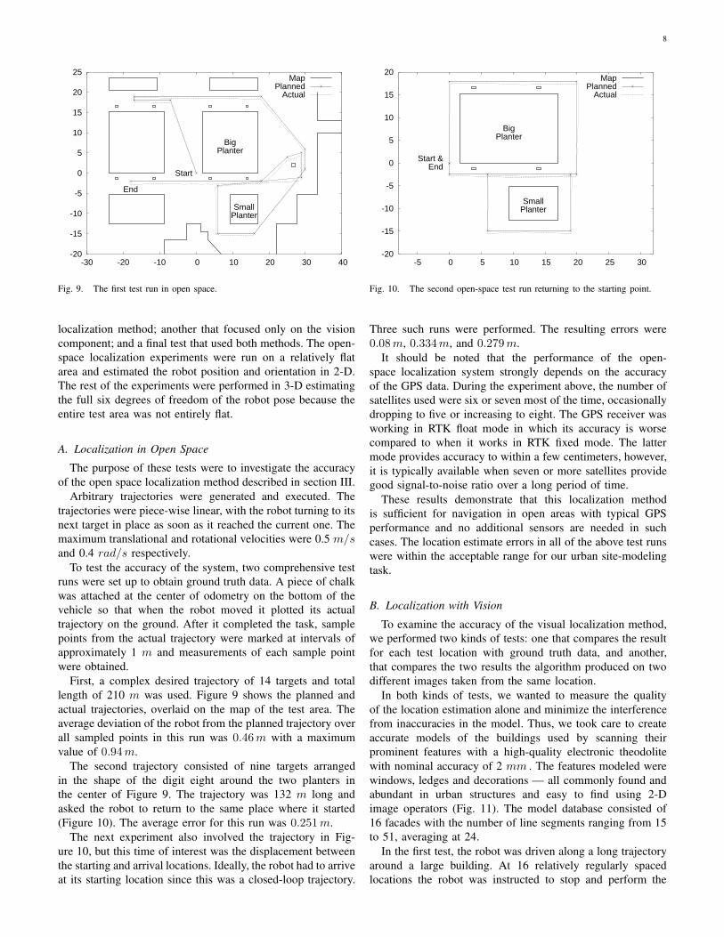
Fig. 9. The first test run in open space.

localization method; another that focused only on the vision

component; and a final test that used both methods. The open-

space localization experiments were run on a relatively flat

area and estimated the robot position and orientation in 2-D.

The rest of the experiments were performed in 3-D estimating

the full six degrees of freedom of the robot pose because the

entire test area was not entirely flat.

A. Localization in Open Space

The purpose of these tests were to investigate the accuracy

of the open space localization method described in section III.

Arbitrary trajectories were generated and executed. The

trajectories were piece-wise linear, with the robot turning to its

next target in place as soon as it reached the current one. The

maximum translational and rotational velocities were 0.5 m/sand 0.4 rad/s respectively.

To test the accuracy of the system, two comprehensive test

runs were set up to obtain ground truth data. A piece of chalk

was attached at the center of odometry on the bottom of the

vehicle so that when the robot moved it plotted its actual

trajectory on the ground. After it completed the task, sample

points from the actual trajectory were marked at intervals of

approximately 1 m and measurements of each sample point

were obtained.

First, a complex desired trajectory of 14 targets and total

length of 210 m was used. Figure 9 shows the planned and

actual trajectories, overlaid on the map of the test area. The

average deviation of the robot from the planned trajectory over

all sampled points in this run was 0.46m with a maximum

value of 0.94m.

The second trajectory consisted of nine targets arranged

in the shape of the digit eight around the two planters in

the center of Figure 9. The trajectory was 132 m long and

asked the robot to return to the same place where it started

(Figure 10). The average error for this run was 0.251m.

The next experiment also involved the trajectory in Fig-

ure 10, but this time of interest was the displacement between

the starting and arrival locations. Ideally, the robot had to arrive

at its starting location since this was a closed-loop trajectory.

-20

-15

-10

-5

0

5

10

15

20

-5 0 5 10 15 20 25 30

BigPlanter

SmallPlanter

Start &End

MapPlanned

Actual

Fig. 10. The second open-space test run returning to the starting point.

Three such runs were performed. The resulting errors were

0.08m, 0.334m, and 0.279m.

It should be noted that the performance of the open-

space localization system strongly depends on the accuracy

of the GPS data. During the experiment above, the number of

satellites used were six or seven most of the time, occasionally

dropping to five or increasing to eight. The GPS receiver was

working in RTK float mode in which its accuracy is worse

compared to when it works in RTK fixed mode. The latter

mode provides accuracy to within a few centimeters, however,

it is typically available when seven or more satellites provide

good signal-to-noise ratio over a long period of time.

These results demonstrate that this localization method

is sufficient for navigation in open areas with typical GPS

performance and no additional sensors are needed in such

cases. The location estimate errors in all of the above test runs

were within the acceptable range for our urban site-modeling

task.

B. Localization with Vision

To examine the accuracy of the visual localization method,

we performed two kinds of tests: one that compares the result

for each test location with ground truth data, and another,

that compares the two results the algorithm produced on two

different images taken from the same location.

In both kinds of tests, we wanted to measure the quality

of the location estimation alone and minimize the interference

from inaccuracies in the model. Thus, we took care to create

accurate models of the buildings used by scanning their

prominent features with a high-quality electronic theodolite

with nominal accuracy of 2 mm . The features modeled were

windows, ledges and decorations — all commonly found and

abundant in urban structures and easy to find using 2-D

image operators (Fig. 11). The model database consisted of

16 facades with the number of line segments ranging from 15

to 51, averaging at 24.

In the first test, the robot was driven along a long trajectory

around a large building. At 16 relatively regularly spaced

locations the robot was instructed to stop and perform the

9

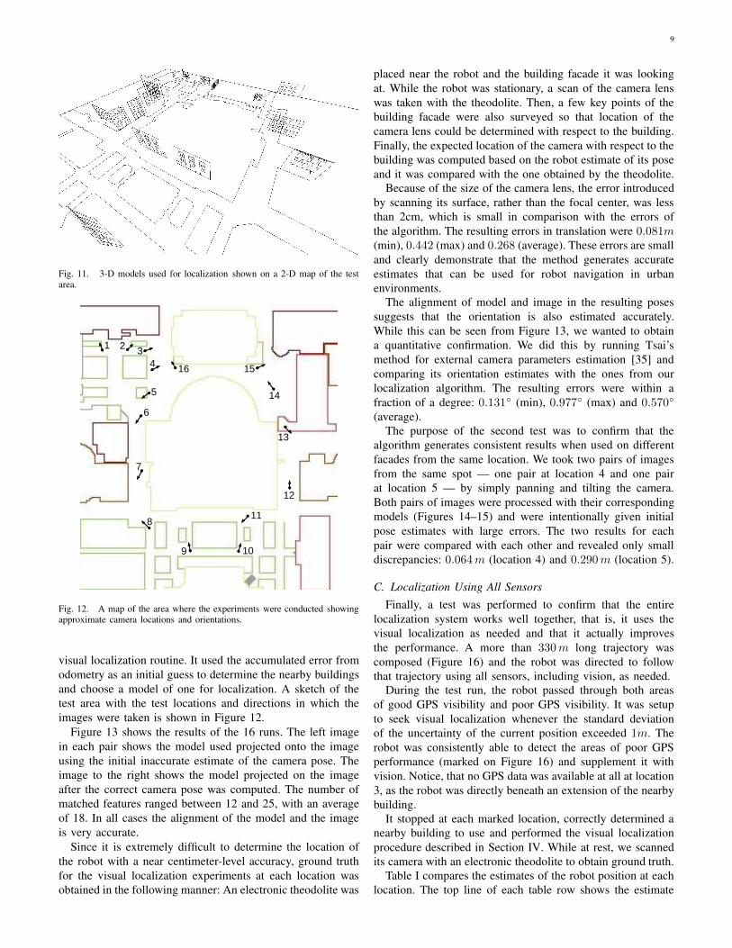
Fig. 11. 3-D models used for localization shown on a 2-D map of the testarea.

1 2 34 16

5

6

7

8

9 10

11

12

13

14

15

Fig. 12. A map of the area where the experiments were conducted showingapproximate camera locations and orientations.

visual localization routine. It used the accumulated error from

odometry as an initial guess to determine the nearby buildings

and choose a model of one for localization. A sketch of the

test area with the test locations and directions in which the

images were taken is shown in Figure 12.

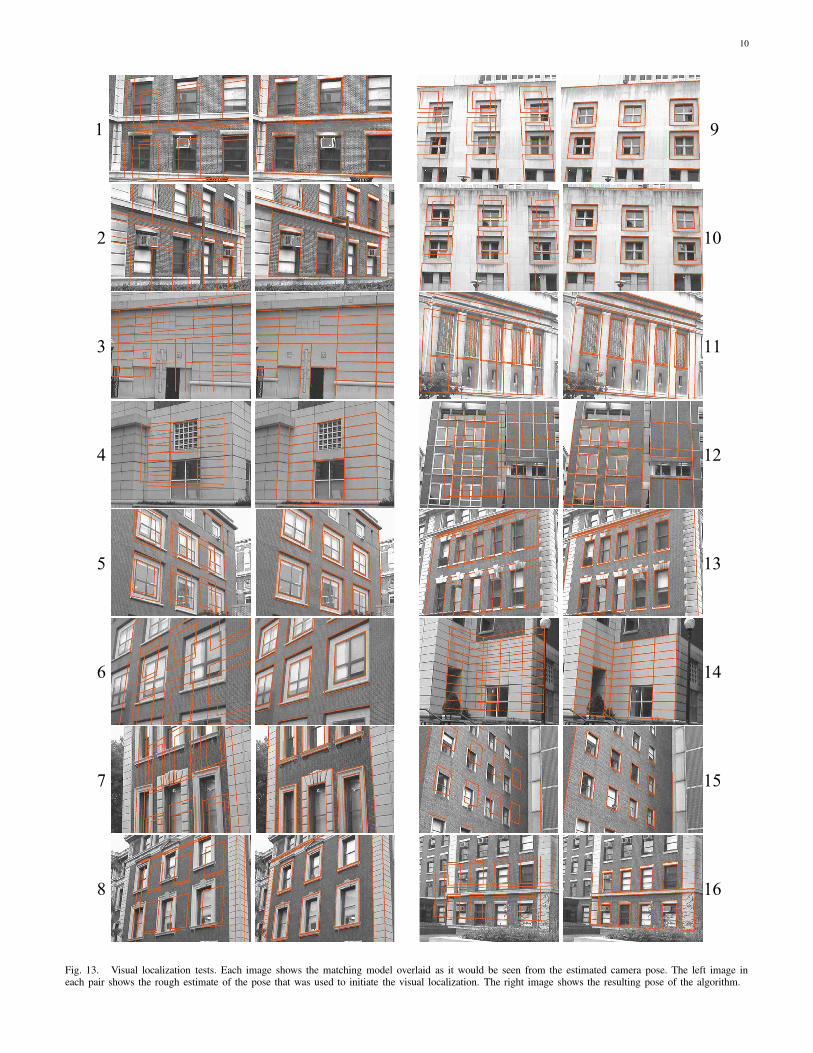
Figure 13 shows the results of the 16 runs. The left image

in each pair shows the model used projected onto the image

using the initial inaccurate estimate of the camera pose. The

image to the right shows the model projected on the image

after the correct camera pose was computed. The number of

matched features ranged between 12 and 25, with an average

of 18. In all cases the alignment of the model and the image

is very accurate.

Since it is extremely difficult to determine the location of

the robot with a near centimeter-level accuracy, ground truth

for the visual localization experiments at each location was

obtained in the following manner: An electronic theodolite was

placed near the robot and the building facade it was looking

at. While the robot was stationary, a scan of the camera lens

was taken with the theodolite. Then, a few key points of the

building facade were also surveyed so that location of the

camera lens could be determined with respect to the building.

Finally, the expected location of the camera with respect to the

building was computed based on the robot estimate of its pose

and it was compared with the one obtained by the theodolite.

Because of the size of the camera lens, the error introduced

by scanning its surface, rather than the focal center, was less

than 2cm, which is small in comparison with the errors of

the algorithm. The resulting errors in translation were 0.081m(min), 0.442 (max) and 0.268 (average). These errors are small

and clearly demonstrate that the method generates accurate

estimates that can be used for robot navigation in urban

environments.

The alignment of model and image in the resulting poses

suggests that the orientation is also estimated accurately.

While this can be seen from Figure 13, we wanted to obtain

a quantitative confirmation. We did this by running Tsai’s

method for external camera parameters estimation [35] and

comparing its orientation estimates with the ones from our

localization algorithm. The resulting errors were within a

fraction of a degree: 0.131◦ (min), 0.977◦ (max) and 0.570◦

(average).

The purpose of the second test was to confirm that the

algorithm generates consistent results when used on different

facades from the same location. We took two pairs of images

from the same spot — one pair at location 4 and one pair

at location 5 — by simply panning and tilting the camera.

Both pairs of images were processed with their corresponding

models (Figures 14–15) and were intentionally given initial

pose estimates with large errors. The two results for each

pair were compared with each other and revealed only small

discrepancies: 0.064m (location 4) and 0.290m (location 5).

C. Localization Using All Sensors

Finally, a test was performed to confirm that the entire

localization system works well together, that is, it uses the

visual localization as needed and that it actually improves

the performance. A more than 330m long trajectory was

composed (Figure 16) and the robot was directed to follow

that trajectory using all sensors, including vision, as needed.

During the test run, the robot passed through both areas

of good GPS visibility and poor GPS visibility. It was setup

to seek visual localization whenever the standard deviation

of the uncertainty of the current position exceeded 1m. The

robot was consistently able to detect the areas of poor GPS

performance (marked on Figure 16) and supplement it with

vision. Notice, that no GPS data was available at all at location

3, as the robot was directly beneath an extension of the nearby

building.

It stopped at each marked location, correctly determined a

nearby building to use and performed the visual localization

procedure described in Section IV. While at rest, we scanned

its camera with an electronic theodolite to obtain ground truth.

Table I compares the estimates of the robot position at each

location. The top line of each table row shows the estimate

10

1 9

2 10

3 11

4 12

5 13

6 14

7 15

8 16

Fig. 13. Visual localization tests. Each image shows the matching model overlaid as it would be seen from the estimated camera pose. The left image ineach pair shows the rough estimate of the pose that was used to initiate the visual localization. The right image shows the resulting pose of the algorithm.

11

Fig. 14. Consistency test 1: Initial and final alignments in the pose estimationtests with a pair of images taken from the same location.

Fig. 15. Consistency test 2: Initial and final alignments in the pose estimationtests with a pair of images taken from the same location.

of the open-space localization method prior to triggering

the visual procedure and its error. The bottom line of the

same row, shows the estimate and the error of the visual

localization. The table clearly demonstrates the improvement

the visual algorithm makes to the overall system performance.

The corresponding images overlaid with the model are shown

in Figure 17.

VI. DISCUSSION AND FUTURE WORK

This paper presented a practical approach to mobile robot

localization in urban environments. The work was done as part

of our AVENUE project for urban site modeling, however,

the methods and ideas presented here are independent of the

project and are generally applicable to mobile robots operating

in urban environments.

The localization system employs the robot odometry, a

digital compass with an integrated tilt sensor, a global po-

sitioning unit, and a camera mounted on a pan-tilt head in

12

3

4start

finish

Fig. 16. A map of the area showing the robot trajectory (dotted line) and thelocations where the robot used visual localization. Notice location 3 which isdirectly underneath a building extension.

TABLE I

ROBOT POSITION AND ERROR ESTIMATED BY GPS, COMPASS AND

ODOMETRY ALONG WITH THE CORRESPONDING IMPROVED POSITION

ESTIMATE AND ERROR AFTER PERFORMING VISUAL LOCALIZATION.

MEASUREMENTS ARE IN METERS.

No Type X Y Z Error

1 Open-space 17.547 -58.079 -0.683 1.297Vision 16.470 -58.565 0.110 0.348

2 Open-space 108.521 -61.634 0.279 1.031Vision 108.260 -62.001 1.127 0.345

3 Open-space 90.660 -30.729 1.418 0.937Vision 91.344 -31.404 0.867 0.179

4 Open-space 95.095 2.577 1.713 1.212Vision 95.363 2.881 0.850 0.274

two complementary ways. The open-space localization method

uses odometry, the digital compass and GPS. The sensor

integration is done by an extended Kalman filter. The method

can be performed in real-time. The visual localization method

is heavier computationally but is only used upon demand. The

pose estimation is done by matching an image of a nearby

building with a simple and compact model. A database of

the models is stored on the on-board computer. No environ-

mental modifications are required. We have demonstrated the

functionality of the robot and the localization methods with

numerous experiments.

Our visual localization method raises an interesting question

about the amount of time it takes on a given mission. This

time is determined by the number of localization efforts as

well as the time spent on each of them (currently, 25–45sec).

The number of visual localization runs depends on a number

of factors, such as the quality of the GPS fixes, the number

of satellites seen, the number, shape and look of the nearby

buildings and the accuracy and completeness of the model.

12

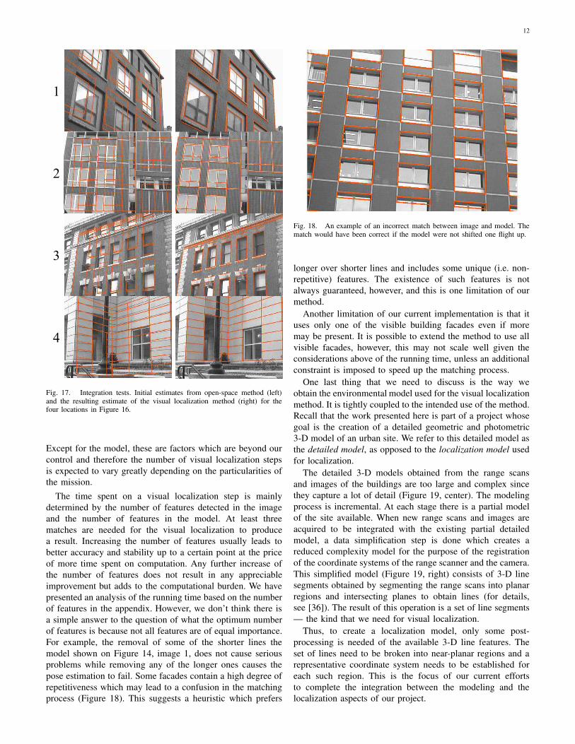
1

2

3

4

Fig. 17. Integration tests. Initial estimates from open-space method (left)and the resulting estimate of the visual localization method (right) for thefour locations in Figure 16.

Except for the model, these are factors which are beyond our

control and therefore the number of visual localization steps

is expected to vary greatly depending on the particularities of

the mission.

The time spent on a visual localization step is mainly

determined by the number of features detected in the image

and the number of features in the model. At least three

matches are needed for the visual localization to produce

a result. Increasing the number of features usually leads to

better accuracy and stability up to a certain point at the price

of more time spent on computation. Any further increase of

the number of features does not result in any appreciable

improvement but adds to the computational burden. We have

presented an analysis of the running time based on the number

of features in the appendix. However, we don’t think there is

a simple answer to the question of what the optimum number

of features is because not all features are of equal importance.

For example, the removal of some of the shorter lines the

model shown on Figure 14, image 1, does not cause serious

problems while removing any of the longer ones causes the

pose estimation to fail. Some facades contain a high degree of

repetitiveness which may lead to a confusion in the matching

process (Figure 18). This suggests a heuristic which prefers

Fig. 18. An example of an incorrect match between image and model. Thematch would have been correct if the model were not shifted one flight up.

longer over shorter lines and includes some unique (i.e. non-

repetitive) features. The existence of such features is not

always guaranteed, however, and this is one limitation of our

method.

Another limitation of our current implementation is that it

uses only one of the visible building facades even if more

may be present. It is possible to extend the method to use all

visible facades, however, this may not scale well given the

considerations above of the running time, unless an additional

constraint is imposed to speed up the matching process.

One last thing that we need to discuss is the way we

obtain the environmental model used for the visual localization

method. It is tightly coupled to the intended use of the method.

Recall that the work presented here is part of a project whose

goal is the creation of a detailed geometric and photometric

3-D model of an urban site. We refer to this detailed model as

the detailed model, as opposed to the localization model used

for localization.

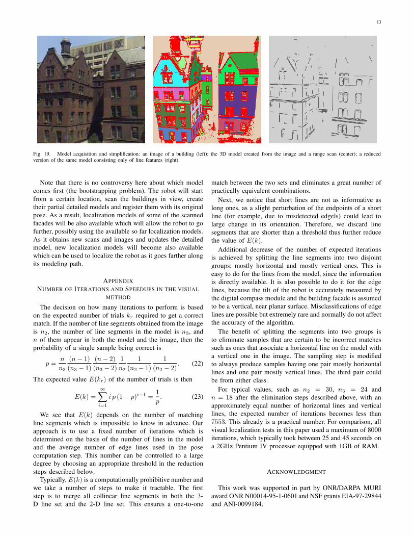
The detailed 3-D models obtained from the range scans

and images of the buildings are too large and complex since

they capture a lot of detail (Figure 19, center). The modeling

process is incremental. At each stage there is a partial model

of the site available. When new range scans and images are

acquired to be integrated with the existing partial detailed

model, a data simplification step is done which creates a

reduced complexity model for the purpose of the registration

of the coordinate systems of the range scanner and the camera.

This simplified model (Figure 19, right) consists of 3-D line

segments obtained by segmenting the range scans into planar

regions and intersecting planes to obtain lines (for details,

see [36]). The result of this operation is a set of line segments

— the kind that we need for visual localization.

Thus, to create a localization model, only some post-

processing is needed of the available 3-D line features. The

set of lines need to be broken into near-planar regions and a

representative coordinate system needs to be established for

each such region. This is the focus of our current efforts

to complete the integration between the modeling and the

localization aspects of our project.

13

Fig. 19. Model acquisition and simplification: an image of a building (left); the 3D model created from the image and a range scan (center); a reducedversion of the same model consisting only of line features (right).

Note that there is no controversy here about which model

comes first (the bootstrapping problem). The robot will start

from a certain location, scan the buildings in view, create

their partial detailed models and register them with its original

pose. As a result, localization models of some of the scanned

facades will be also available which will allow the robot to go

further, possibly using the available so far localization models.

As it obtains new scans and images and updates the detailed

model, new localization models will become also available

which can be used to localize the robot as it goes farther along

its modeling path.

APPENDIX

NUMBER OF ITERATIONS AND SPEEDUPS IN THE VISUAL

METHOD

The decision on how many iterations to perform is based

on the expected number of trials kr required to get a correct

match. If the number of line segments obtained from the image

is n2, the number of line segments in the model is n3, and

n of them appear in both the model and the image, then the

probability of a single sample being correct is

p =n

n3

(n− 1)

(n3 − 1)

(n− 2)

(n3 − 2)

1

n2

1

(n2 − 1)

1

(n2 − 2). (22)

The expected value E(kr) of the number of trials is then

E(k) =

∞∑

i=1

i p (1− p)i−1 =1

p. (23)

We see that E(k) depends on the number of matching

line segments which is impossible to know in advance. Our

approach is to use a fixed number of iterations which is

determined on the basis of the number of lines in the model

and the average number of edge lines used in the pose

computation step. This number can be controlled to a large

degree by choosing an appropriate threshold in the reduction

steps described below.

Typically,E(k) is a computationally prohibitive number and

we take a number of steps to make it tractable. The first

step is to merge all collinear line segments in both the 3-

D line set and the 2-D line set. This ensures a one-to-one

match between the two sets and eliminates a great number of

practically equivalent combinations.

Next, we notice that short lines are not as informative as

long ones, as a slight perturbation of the endpoints of a short

line (for example, due to misdetected edgels) could lead to

large change in its orientation. Therefore, we discard line

segments that are shorter than a threshold thus further reduce

the value of E(k).

Additional decrease of the number of expected iterations

is achieved by splitting the line segments into two disjoint

groups: mostly horizontal and mostly vertical ones. This is

easy to do for the lines from the model, since the information

is directly available. It is also possible to do it for the edge

lines, because the tilt of the robot is accurately measured by

the digital compass module and the building facade is assumed

to be a vertical, near planar surface. Misclassifications of edge

lines are possible but extremely rare and normally do not affect

the accuracy of the algorithm.

The benefit of splitting the segments into two groups is

to eliminate samples that are certain to be incorrect matches

such as ones that associate a horizontal line on the model with

a vertical one in the image. The sampling step is modified

to always produce samples having one pair mostly horizontal

lines and one pair mostly vertical lines. The third pair could

be from either class.

For typical values, such as n2 = 30, n3 = 24 and

n = 18 after the elimination steps described above, with an

approximately equal number of horizontal lines and vertical

lines, the expected number of iterations becomes less than

7553. This already is a practical number. For comparison, all

visual localization tests in this paper used a maximum of 8000

iterations, which typically took between 25 and 45 seconds on

a 2GHz Pentium IV processor equipped with 1GB of RAM.

ACKNOWLEDGMENT

This work was supported in part by ONR/DARPA MURI

award ONR N00014-95-1-0601 and NSF grants EIA-97-29844

and ANI-0099184.

14

REFERENCES

[1] P. Allen, I. Stamos, A. Gueorguiev, E. Gold, and P. Blaer, “AVENUE:Automated site modeling in urban environments,” in Proceedings of 3rd

Conference on Digital Imaging and Modeling in Quebec City, Canada,May 2001, pp. 357–364.

[2] J. Borenstein and L. Feng, “Correction of systematic odometry errorsin mobile robots,” in IROS’95, Pittsburgh, Pennsylvania, August 1995,pp. 569–574.

[3] ——, “Gyrodometry: A new method for combining data from gyrosand odometry in mobile robots,” in Proceedings of IEEE International

Conference on Robotics and Automation in Minneapolis, Minnesota,1996, pp. 423–428.

[4] S. I. Roumeliotis, G. S. Sukhatme, and G. A. Bakey, “Circumventingdynamic modeling: Evaluation of the error-state Kalman Filter appliedto mobile robot localization,” in Proceedings of IEEE International

Conference on Robotics and Automation in Detroit, Michigan, 1999,pp. 1656–1663.

[5] S. Cooper and H. F. Durrant-Whyte, “A Kalman filter model for GPSnavigation of land vehicles,” in Proceedings of IEEE International

Conference on Robotics and Automation in San Diego, California, 1994,pp. 157–163.

[6] J. Schleppe, “Development of a real-time attitude system using aquaternion parametrization and non-dedicated GPS receivers,” Master’sthesis, Department of Geomatics Engineering, University of Calgary,Canada, 1996.

[7] T. Aono, K. Fujii, S. Hatsumoto, and T. Kamiya, “Positioning of vehicleon undulating ground using GPS and dead reckoning,” in Proceedings ofIEEE International Conference on Robotics and Automation in Leuven,

Belgium, 1998, pp. 3443–3448.

[8] C.-C. Lin and R. L. Tummala, “Mobile robot navigation using artificiallandmarks,” Journal of Robotics Systems, vol. 14, no. 2, pp. 93–106,1997.

[9] S. Thrun, “Finding landmarks for mobile robot navigation,” in Proceed-ings of IEEE International Conference on Robotics and Automation in

Leuven, Belgium, 1998, pp. 958–963.[10] R. Sim and G. Dudek, “Mobile robot localization from learned land-

marks,” in Proceedings of IEEE/RSJ International Conference on Intel-

ligent Robots and Systems in Victoria, BC, Canada, October 1998.[11] A. Kosaka and A. C. Kak, “Fast vision-guided mobile robot navigation

using model-based reasoning and prediction of uncertainties,” Com-

puter Vision, Graphics, and Image Processing — Image Understanding,vol. 56, no. 3, pp. 271–329, 1992.

[12] M. Bozorg, E. Nebot, and H. Durrant-Whyte, “A decentralised naviga-tion architecture,” in Proceedings of IEEE International Conference on

Robotics and Automation in Leuven, Belgium, 1998, pp. 3413–3418.[13] J. Neira, J. Tardos, J. Horn, and G. Schmidt, “Fusing range and intensity

images for mobile robot localization,” IEEE Transactions on Robotics

and Automation, vol. 15, no. 1, pp. 76–84, February 1999.[14] J. Castellanos and J. Tardos, Mobile Robot Localization and Map Build-

ing: A Multisensor Fusion Approach. Kluwer Academic Publishers,1999.

[15] S. Thrun, W. Burgard, and D. Fox, “A probabilistic approach toconcurrent mapping and localization for mobile robots,” Autonomous

Robots, vol. 5, pp. 253–271, 1998.[16] F. Dellaert, D. Fox, W. Burgard, and S. Thrun, “Monte Carlo localization

for mobile robots,” in Proceedings of IEEE International Conference on

Robotics and Automation in Detroit, Michigan, 1999, pp. 1322–1328.[17] H. Durrant-Whyte, G. Dissanayake, and P. Gibbens, “Toward deploy-

ment of large scale simultaneous localization and map building (SLAM)systems,” in Proceedings of International Simposium on Robotics Re-search in Salt Lake City, Utah, 1999, pp. 121–127.

[18] J. Leonard and H. J. S. Feder, “A computationally efficient methodfor large-scale concurrent mapping and localization,” in Proceedings ofInternational Simposium on Robotics Research in Salt Lake City, Utah,1999, pp. 128–135.

[19] J. Borenstein and L. Feng, Navigating Mobile Robots: Systems and

Techniques. A. K. Peters, 1996.

[20] H. R. Everett, Sensors for Mobile Robots: Theory and Application.Wellesley, Massachusetts: A. K. Peters, 1995.

[21] D. Kortenkamp, R. P. Bonasso, and R. Murphy, Eds., Artificial Intelli-

gence and Mobile Robots: Case Studies of Successful Robot Systems.AAAI Press / The MIT Press, 1998.

[22] G. Dissanayake, P. Newman, S. Clark, H. Durrant-Whyte, andM. Csorba, “A solution to the simultaneous localisation and map building(SLAM) problem,” IEEE Transactions on Robotics and Automation,vol. 17, no. 3, pp. 229–241, June 2001.

[23] J. Guivant, E. Nebot, and H. Durrant-Whyte, “Simultaneous localizationand map bulding using natural features in outdoor environments,”Intelligent Autonomous Systems 6, vol. 1, pp. 581–588, July 2000.

[24] R. Talluri and J.K.Aggarwal, “Mobile robot self-location using model-image feature correspondence,” IEEE Transactions on Robotics and

Automation, vol. 12, no. 1, pp. 63–77, February 1996.[25] T. Chen and R. Shibasaki, “High precision navigation for 3-D mobile

GIS in urban area by integrating GPS, gyro and image sequenceanalysis,” in Proceedings of the International Workshop on Urban

3D/Multi-media Mapping, Tokyo, Japan, 1999, pp. 147–156.[26] R. Nayak, “Reliable and continuous urban navigation using multiple

GPS antennas and a low cost IMU,” Master’s thesis, Department ofGeomatics Engineering, University of Calgary, Canada, 2000.

[27] I. Stamos, “Geometry and texture recovery of scenes of large scale,”Journal of Computer Vision and Image Understanding, vol. 88, no. 2,pp. 94–118, November 2002.

[28] P. Blaer, “Robot path planning using generalized voronoi diagrams,”http://www.cs.columbia.edu/˜pblaer/projects/path planner.

[29] E. Gold, “AvenueUI: A comprehensive visualization/teleoperation appli-cation and development framework for multiple mobile robots,” Master’sthesis, Columbia University, Department of Computer Science, 2001.

[30] R. Brown and P. Hwang, Introduction to random signals and appliedKalman filtering, 3rd ed. John Wiley & Sons, 1997.

[31] A. Georgiev, “Design, implementation and localization of a mobile robotfor urban site modeling,” Ph.D. dissertation, Columbia University, NewYork, NY, 2003.

[32] M. Fischler and R. Bolles, “Random sample consensus: A paradigmfor model fitting with applications to image analysis and automatedcartography,” in DARPA, 1980, pp. 71–88.

[33] R. Kumar and A. R. Hanson, “Robust methods for estimating pose and asensitivity analysis,” Computer Vision Graphics and Image Processing,vol. 60, no. 3, pp. 313–342, November 1994.

[34] B. K. P. Horn, “Relative orientation,” International Journal of Computer

Vision, vol. 4, no. 1, pp. 59–78, 1990.[35] R. Y. Tsai, “A versatile camera calibration technique for high-accuracy 3-

D machine vision metrology using off-the-shelf TV cameras and lenses,”Journal of Robotics and Automation, vol. RA-3, no. 4, pp. 323–344,1987.

[36] I. Stamos and P. K. Allen, “Integration of range and image sensingfor photorealistic 3D modeling,” in Proceedings of IEEE InternationalConference on Robotics and Automation in San Francisco, California,2000, pp. II:1435–1440.

Atanas Georgiev is a postdoctoral research scientistat Columbia University. He graduated with the M.S.degree in Computer Science from Sofia University“St. Kliment Ohridski”, Sofia, Bulgaria . He receivedthe M.S., M.Phil. and Ph.D. degrees in ComputerScience from Columbia University. His current re-search interests are in the areas of mobile robots androbotic micromanipulation.

Peter K. Allen is professor of Computer Science atColumbia University. He received the A.B. degreefrom Brown University in Mathematics-Economics,the M.S. in Computer Science from the Univeristyof Oregon and the Ph.D. in Computer Science fromthe University of Pennsylvania. His current researchinterests include real-time computer vision, dextrousrobotic hands, 3-D modeling and sensor planning.In recognition of his work, Professor Allen hasbeen named a Presidential Young Investigator by theNational Science Foundation.