Local structures;Causal Independence,

Context-sepcific independanceCOMPSCI 276

Fall 2007

Local structure 2

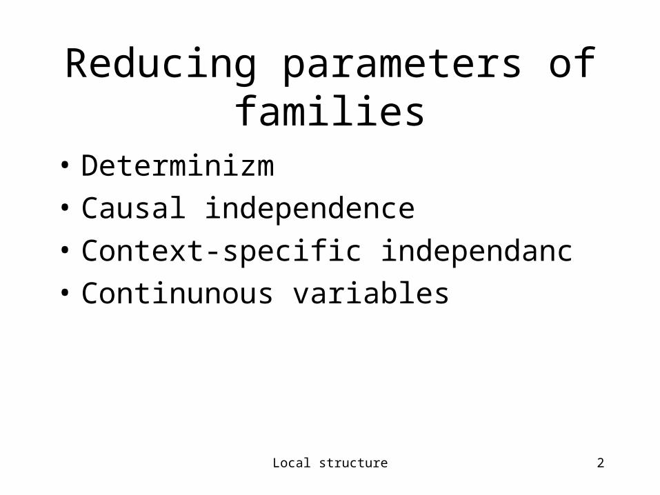
Reducing parameters of families

• Determinizm

• Causal independence

• Context-specific independanc

• Continunous variables

Local structure 3

Local structure 4

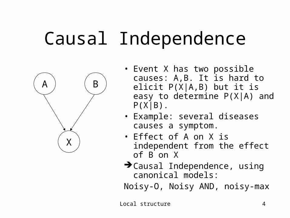
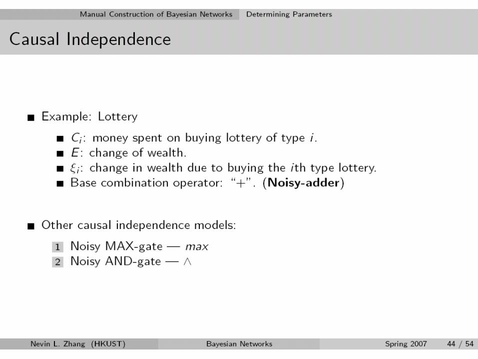
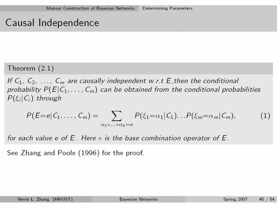
Causal Independence

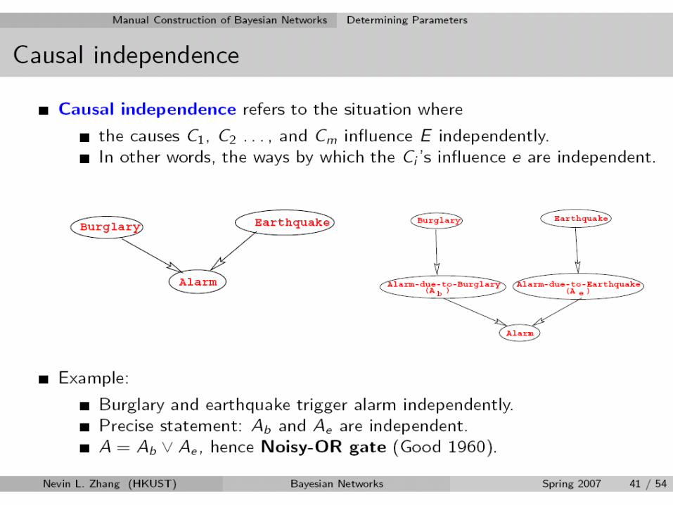
• Event X has two possible causes: A,B. It is hard to elicit P(X|A,B) but it is easy to determine P(X|A) and P(X|B).

• Example: several diseases causes a symptom.

• Effect of A on X is independent from the effect of B on X

Causal Independence, using canonical models:

Noisy-O, Noisy AND, noisy-max

A B

X

Local structure 5

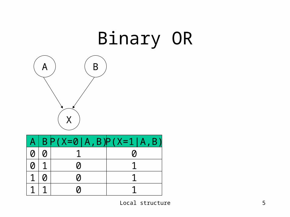
Binary OR

A B

X

A B P(X=0|A,B)0 0 1

P(X=1|A,B)0

0 1 0 11 0 0 11 1 0 1

Local structure 6

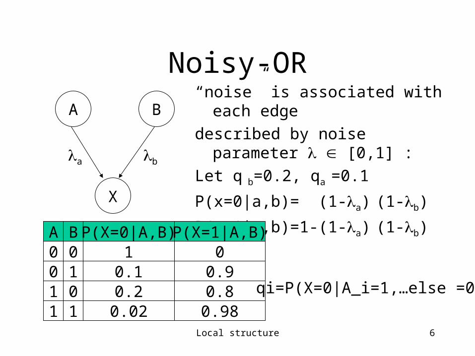
Noisy-OR“noise” is associated with each edge

described by noise parameter [0,1] :

Let q b=0.2, qa =0.1

P(x=0|a,b)= (1-a) (1-b)

P(x=1|a,b)=1-(1-a) (1-b)

A B

X

A B P(X=0|A,B)0 0 1

P(X=1|A,B)0

a b

0 1 0.1 0.91 0 0.2 0.81 1 0.02 0.98

qi=P(X=0|A_i=1,…else =0)

Local structure 7

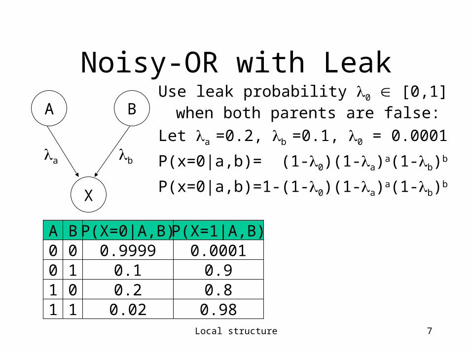
Noisy-OR with LeakUse leak probability 0 [0,1] when both

parents are false:

Let a =0.2, b =0.1, 0 = 0.0001

P(x=0|a,b)= (1-0)(1-a)a(1-b)b

P(x=0|a,b)=1-(1-0)(1-a)a(1-b)b

A B

X

A B P(X=0|A,B)0 0 0.9999

P(X=1|A,B)0.0001

a b

0 1 0.1 0.91 0 0.2 0.81 1 0.02 0.98

Local structure 9

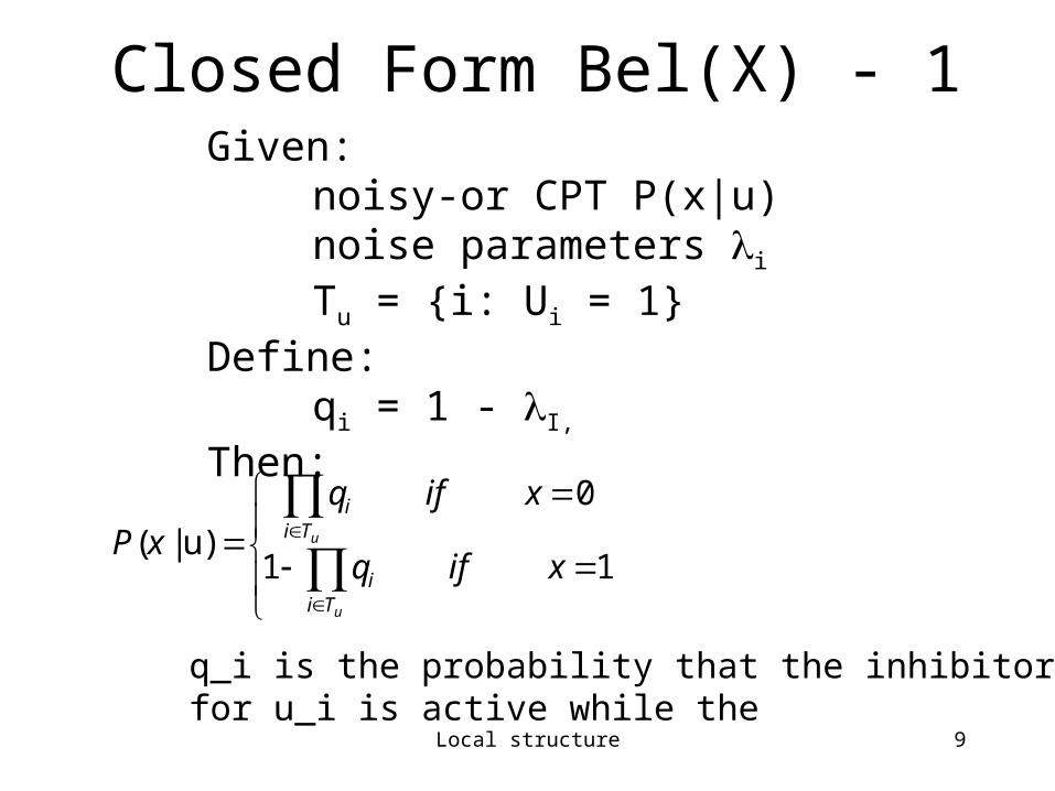
Closed Form Bel(X) - 1

u

u

Tii

Tii

xifq

xifq

xP11

0

)u|(

Given: noisy-or CPT P(x|u)

noise parameters i

Tu = {i: Ui = 1}Define:

qi = 1 - I,

Then:

q_i is the probability that the inhibitor for u_i is active while the

Local structure 11

Closed Form Bel(X) - 2Using Iterative Belief Propagation:

k

kxu

uuxPxxBEL )()|()()(

u

u

Ti kkxi

u

Ti kkxi

u

xifuq

xifuq

xBEL1)()1(

0)(

)(1

0

Set piix = pix (uk=1). Then we can show that:

1)1(1

0)1(

)(1

0

xif

xif

xBEL

iixi

iixi

Local structure 12

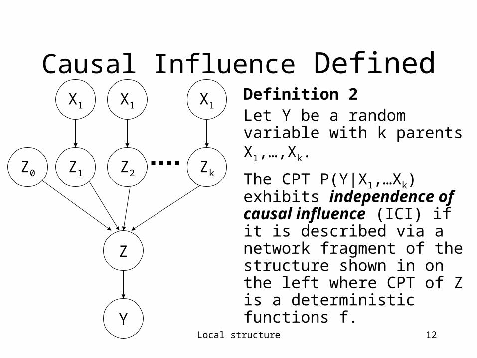
Causal Influence DefinedDefinition 2Let Y be a random variable with k parents X1,…,Xk.

The CPT P(Y|X1,…Xk) exhibits independence of causal influence (ICI) if it is described via a network fragment of the structure shown in on the left where CPT of Z is a deterministic functions f.

Z

Y

X1 X1 X1

Z0 Z1 Z2 Zk

Local structure 13

Local structure 14

Local structure 15

Local structure 16

Local structure 17

Local structure 18

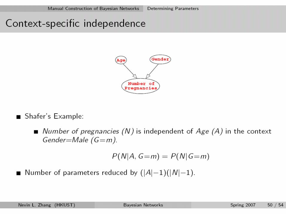
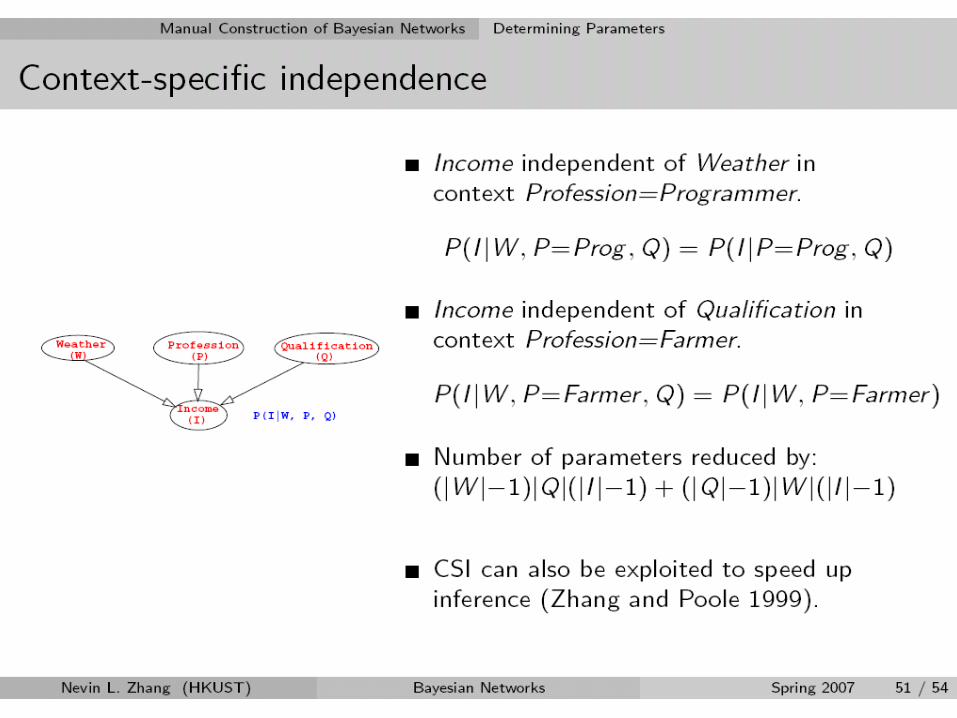
Context Specific Independence

• When there is conditional independence in some specific variable assignment

Local structure 19

Local structure 20

Local structure 21

Local structure 22

Local structure 23

The impact during inference

• Causal independence in polytrees is linear during inference

• Causal independence in general can sometime be exploited but not always

• CSI can be exploited by using operation (product and summation) over trees.

Local structure 24

Representing CSI

• Using decision trees

• Using decision graphs

Local structure 25

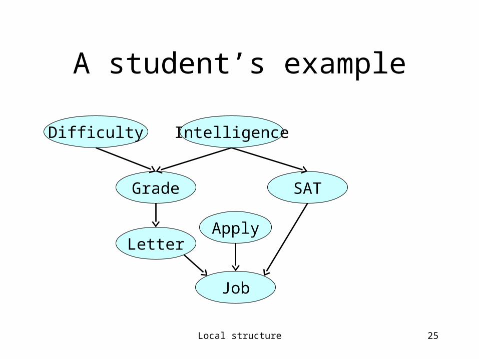
IntelligenceDifficulty

Grade

Letter

SAT

Job

Apply

A student’s example

Local structure 26

A

S

L

(0.8,0.2)

(0.9,0.1) (0.4,0.6)

(0.1,0.9)

s1

a0 a1

s0

l1l0

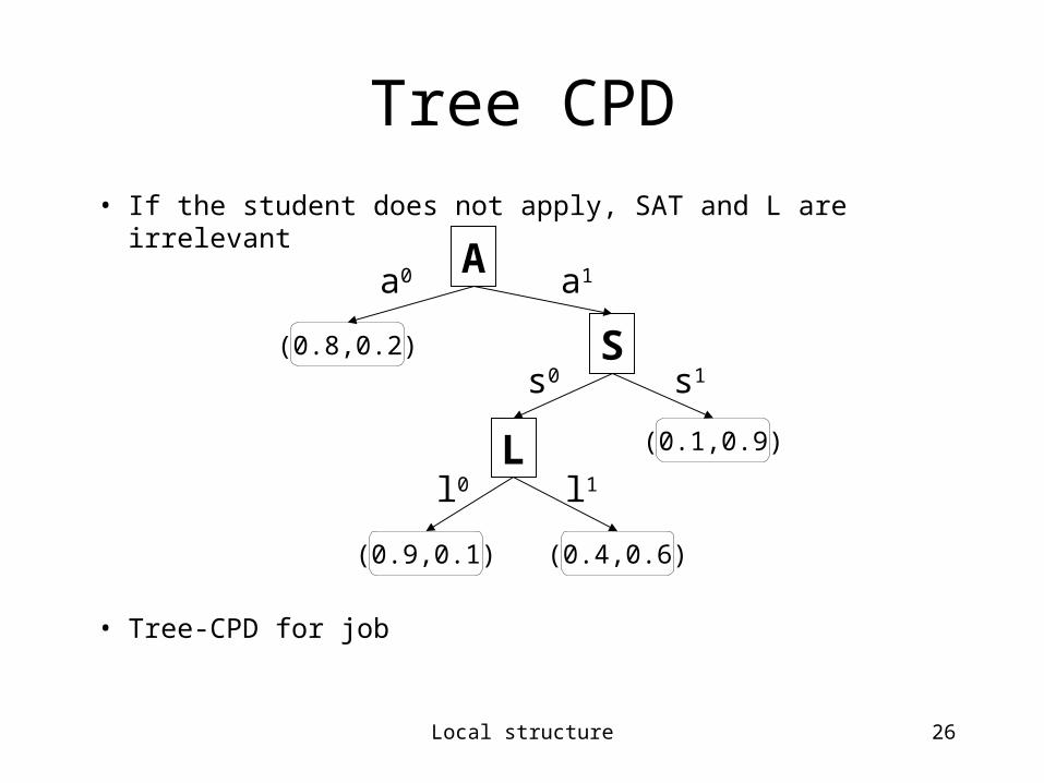
Tree CPD

• If the student does not apply, SAT and L are irrelevant

• Tree-CPD for job

Local structure 27

Definition of CPD-tree

• A CPD-tree of a CPD P(Z|pa_Z) is a tree whose leaves are labeled by P(Z) and internal nodes correspond to parents branching over their values.

Local structure 28

C

L2

(0.1,0.9)

l21

c1 c2

l20L1

(0.8,0.2)(0.3,0.7)

l11l10

(0.9,0.1)

Letter1

Job

Letter2

Choice

Captures irrelevant variables

Local structure 29

Multiplexer CPD

• A CPD P(Y|A,Z1,Z2,…,Zk) is a multiplexer iff Val(A)=1,2,…k, and

• P(Y|A,Z1,…Zk)=Z_a

Letter1

Letter

Letter2

Choice

Job

Local structure 30

A

B

C

(0.3,0.7) (0.4,0.6)

(0.1,0.9)

b1

a0 a1

b0

c1c0

C

B

(0.3,0.7) (0.5,0.5)

(0.2,0.8)

c1c0

b1b0

Rule-based representation• A CPD-tree that correponds to rules.

Local structure 32

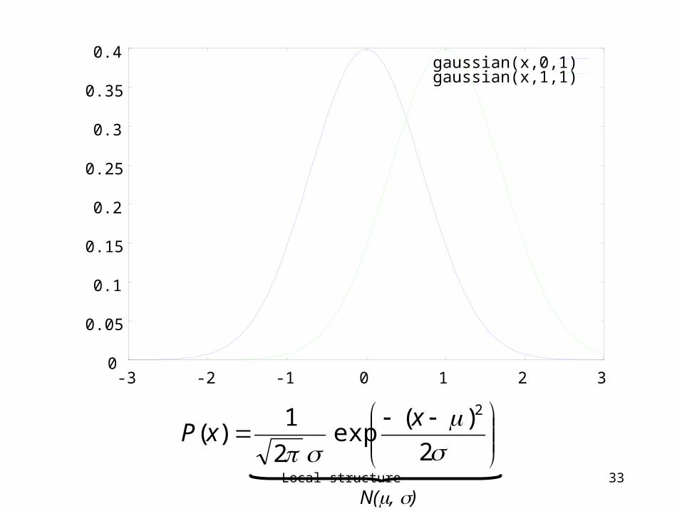
Gaussian Distribution

2

)(exp

2

1)(

2xxP

N(, )

Local structure 33

0

0.05

0.1

0.15

0.2

0.25

0.3

0.35

0.4

-3 -2 -1 0 1 2 3

gaussian(x,0,1)gaussian(x,1,1)

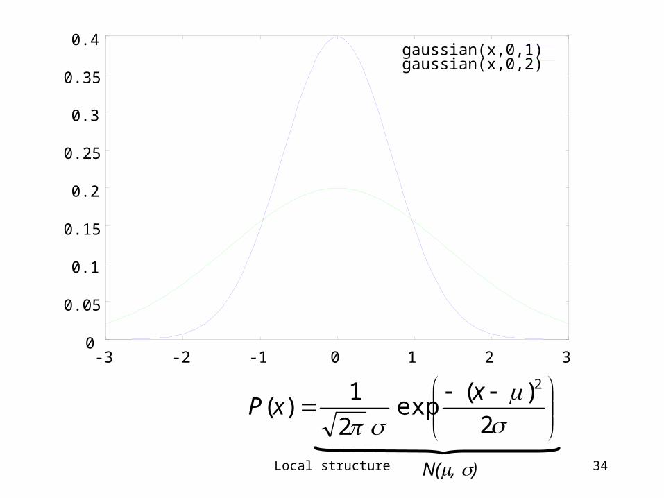
2

)(exp

2

1)(

2xxP

N(, )

Local structure 34

0

0.05

0.1

0.15

0.2

0.25

0.3

0.35

0.4

-3 -2 -1 0 1 2 3

gaussian(x,0,1)gaussian(x,0,2)

2

)(exp

2

1)(

2xxP

N(, )

Local structure 35

Multivariate GaussianDefinition:

Let X1,…,Xn. Be a set of random variables. A multivariate Gaussian distribution over X1,…,Xn is a parameterized by an n-dimensional mean vector and an n x n positive definitive covariance matrix . It defines a joint density via:

)()(

2

1

||)2(

1)( 1

2/12/

xxXP T

n

Local structure 36

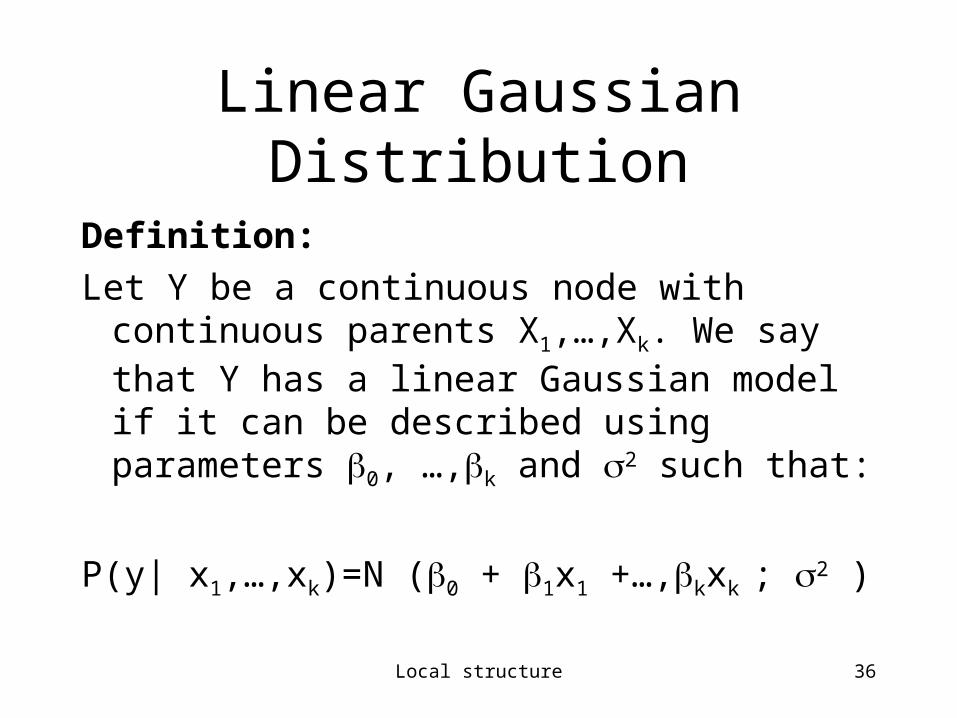
Linear Gaussian Distribution

Definition:

Let Y be a continuous node with continuous parents X1,…,Xk. We say that Y has a linear Gaussian model if it can be described using parameters 0, …,k and 2 such that:

P(y| x1,…,xk)=N (0 + 1x1 +…,kxk ; 2 )

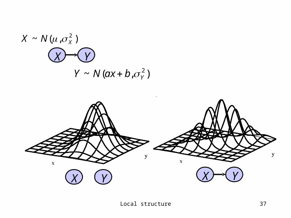
Local structure 37

X Y

),(~ 2XNX

),(~ 2YbaxNY

X YX Y

Local structure 38

kkYY 110

-10 -5 0 5 10X -10-5

05

10

Y

00.050.10.150.20.250.30.350.4

Local structure 39

Linear Gaussian NetworkDefinition

Linear Gaussian Bayesian network is a Bayesian network all of whose variables are continuous and where all of the CPTs are linear Gaussians.

Linear Gaussian BN Multivariate Gaussian

=>Linear Gaussian BN has a compact representation

Local structure 40

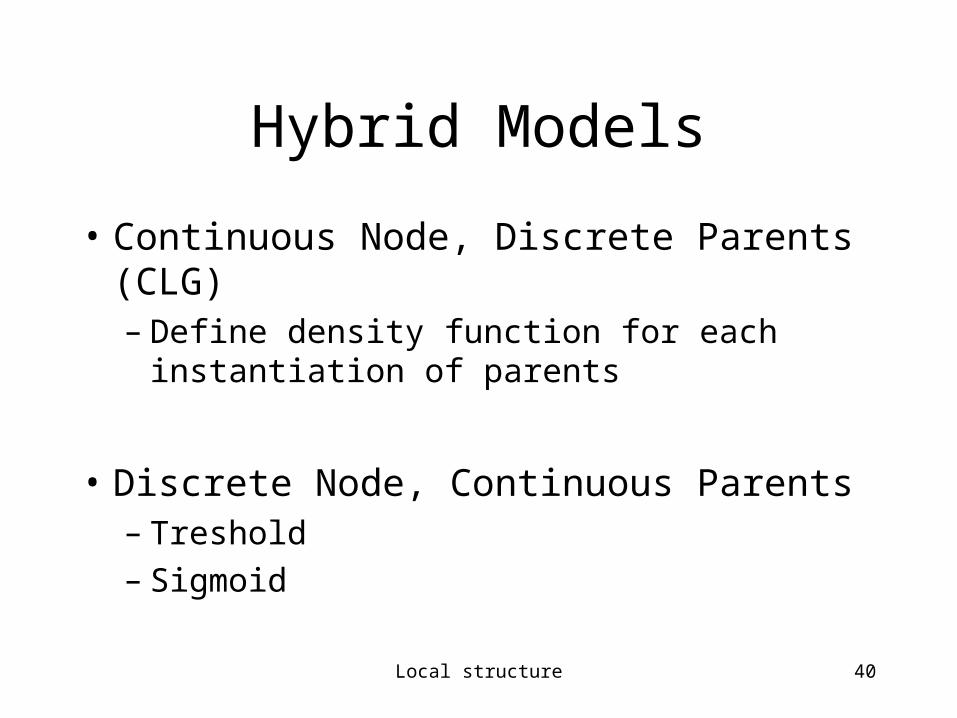
Hybrid Models

• Continuous Node, Discrete Parents (CLG)– Define density function for each instantiation of

parents

• Discrete Node, Continuous Parents– Treshold– Sigmoid

Local structure 41

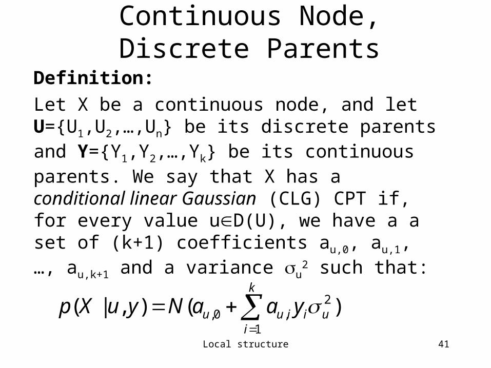
Continuous Node, Discrete Parents

Definition:

Let X be a continuous node, and let U={U1,U2,…,Un} be its discrete parents and Y={Y1,Y2,…,Yk} be its continuous parents. We say that X has a conditional linear Gaussian (CLG) CPT if, for every value uD(U), we have a a set of (k+1) coefficients au,0, au,1, …, au,k+1 and a variance u

2 such that:)(),|(

1

2,0,

k

iuiiuu yaaNyuXp

Local structure 42

CLG Network

Definition:

A Bayesian network is called a CLG network if every discrete node has only discrete parents, and every continuous node has a CLG CPT.

Local structure 43

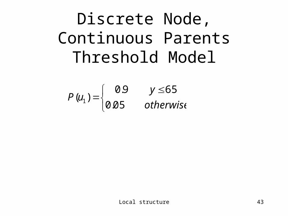
Discrete Node, Continuous ParentsThreshold Model

otherwise

yuP

05.0

659.0)( 1

Local structure 44

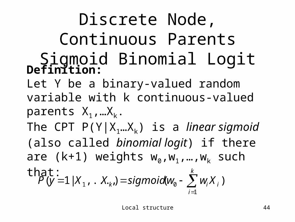
Discrete Node, Continuous ParentsSigmoid Binomial Logit

k

iiik XwwsigmoidXXyP

101 )(),...,|1(

Definition:Let Y be a binary-valued random variable with k continuous-valued parents X1,…Xk. The CPT P(Y|X1…Xk) is a linear sigmoid (also called binomial logit) if there are (k+1) weights w0,w1,…,wk such that:

Local structure 45

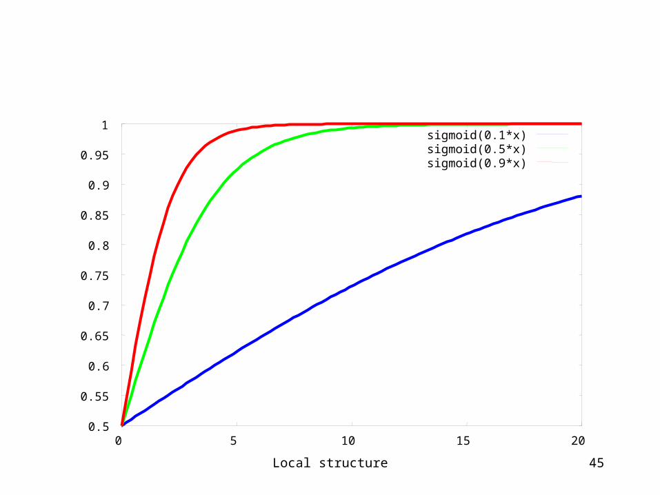
0.5

0.55

0.6

0.65

0.7

0.75

0.8

0.85

0.9

0.95

1

0 5 10 15 20

sigmoid(0.1*x)sigmoid(0.5*x)sigmoid(0.9*x)

Local structure 46

References

• Judea Pearl “Probabilistic Reasoning in Inteeligent Systems”, section 4.3

• Nir Friedman, Daphne Koller “Bayesian Network and Beyond”