LOCAL REVENUE HILLS: A GENERAL EQUILIBRIUM SPECIFICATION W1TH EVIDENCE FROM … · · 2002-09-17A...
62
NBER WORKING PAPER SERIES LOCAL REVENUE HILLS: A GENERAL EQUILIBRIUM SPECIFICATION W1TH EVIDENCE FROM POUR U.S. CiTIES Andrew Haughwout Robert Inman Steven Craig Thomas Luce Working Paper 7603 http://www.nber.org/papers/w7603 NATIONAL BUREAU OP ECONOMIC RESEARCH 1050 Massachusetts Avenue Cambridge, MA 02138 March 2000 The authors would like to thank the Zell Center for Real Estate Research, Wharton School, University of Pennsylvania for financial support. Haughwout and Inman also received support from the National Science Foundation. The comments of Howard Chernick, Joe Gyourko, Todd Sinai, Anita Summers, and John Quigley are appreciated as are those of seminar participants at Princeton University, the Wharton School, the ZEW Federalism Conference, the Norwegian Tax Forum 1999, the NBER Summer Institute Public Finance Workshop, and the 1999 Meetings of the American Public Policy and Management Association. The views expressed herein are those of the authors and not necessarily those of the National Bureau of Economic Research or the Federal Reserve Bank of New York. 2000 by Andrew Haughwout, Robert Inman, Steven Craig, and Thomas Luce. All rights reserved. Short sections of text, not to exceed two paragraphs, may be quoted without explicit permission provided that full credit, including notice, is given to the source.
-
Upload
nguyenliem -
Category
Documents
-
view
219 -
download
0
Transcript of LOCAL REVENUE HILLS: A GENERAL EQUILIBRIUM SPECIFICATION W1TH EVIDENCE FROM … · · 2002-09-17A...
NBER WORKING PAPER SERIES
LOCAL REVENUE HILLS:A GENERAL EQUILIBRIUM SPECIFICATION W1TH
EVIDENCE FROM POUR U.S. CiTIES
Andrew HaughwoutRobert InmanSteven CraigThomas Luce
Working Paper 7603http://www.nber.org/papers/w7603
NATIONAL BUREAU OP ECONOMIC RESEARCH1050 Massachusetts Avenue
Cambridge, MA 02138March 2000
The authors would like to thank the Zell Center for Real Estate Research, Wharton School, University of Pennsylvaniafor financial support. Haughwout and Inman also received support from the National Science Foundation. Thecomments of Howard Chernick, Joe Gyourko, Todd Sinai, Anita Summers, and John Quigley are appreciated as arethose of seminar participants at Princeton University, the Wharton School, the ZEW Federalism Conference, theNorwegian Tax Forum 1999, the NBER Summer Institute Public Finance Workshop, and the 1999 Meetings of theAmerican Public Policy and Management Association. The views expressed herein are those of the authors and notnecessarily those of the National Bureau of Economic Research or the Federal Reserve Bank of New York.
2000 by Andrew Haughwout, Robert Inman, Steven Craig, and Thomas Luce. All rights reserved. Short sectionsof text, not to exceed two paragraphs, may be quoted without explicit permission provided that full credit, including
notice, is given to the source.

Local Revenue Hills:
A General Equilibrium Specification with Evidence from Four U.S. Cities
by
Andrew Haughwout, Robert Inman, Steven Craig, Thomas Luce'
Adam Smith: High taxes, sometimes by diminishing consumption of the taxedcommodities, and sometimes by encouraging smuggling, frequently afford a smallerrevenue to government than what might be drawn from more moderate. taxes. (FromAdam Smith, The Wealth of Nations, book V, Chapter II.)
Alexander Hamilton: It is a signal advantage of taxes on articles of consumption that theycontain in their own nature a security against excess. . . . If duties are too high, theylessen the consumption; the collection is eluded; and the product to the treasury is notso great as when they are confined within proper and moderate bounds. (From "FurtherDefects of the Present Constitution," Federalist Papers, No. 21.)
Jules Dupuit: Ifa tax is gradually increased from zero up to the point where it becomeprohibitive, its yield is at first nil, then increase by small stages until it reaches amaximum, after which it gradually declines until it becomes zero again. (From JulesDupuit, "On the Measurement of Utility from Public Works," reprinted, in K. Arrowand Tibor Scitovsky (1969), Readings in Welfare Economics, Homewood, Ii: Richard D.Irwin.)
John Maynard Keynes: Nor should the argument seem strange that taxation may be sohigh as to defeat its object, and that, given sufficient time to gather the fruits, a reductionof taxation will run a better chance than increase of balancing the budget. (From JohnMaynard Keynes, Collected Works of John Maynard Keynes, St. Martin's Press, p. 338.)

Local Revenue Hills: A General Equilibrium Specification with Evidencefrom Pour U.S. CitiesAndrew Haughwout, Robert Inman, Steven Craig, and Thomas LuceNBER Working Paper No. 7603March 2000JELN0. H2, H71, R5l
ABSTRACT
We provide estimates of the impact and long-run elasticities of tax base with respect to tax
rates for four large U.S. cities: Houston (property taxation), Minneapolis (property taxation), New
York City (property, general sales, and income taxation), and Philadelphia (property, gross receipts,
and wage taxation). Results suggest that all four of our cities are near the peaks of their longer-mn
revenue hills. Equilibrium effects are observed within three to four fiscal years after the initial
increase in local, tax rates. A significant negative impact (current period) effect of a balanced budget
increase in city property tax rates on city property base is interpreted as a capitalization effect and
suggests that marginal increases in city spending do not provide positive net benefits to property
owners. Estimates of the effects of taxes on city employment levels for New York City and
Philadelphia — the two cities for which employment series are available —show the local income and
wage tax rates have significant negative effects on city employment levels.
Andrew Haughwout Robert InmanDomestic Research Department Finance DepartmentFederal Reserve Bank of New York Wharton SchoolNew York, NY 10045 University of [email protected] Philadelphia, PA 19104
and NBERinman @wharton.upenn.edu
Steven Craig Thomas LuceDepartment of Economics Hubert Humphrey School of Public PolicyUniversity of Houston University of MinnesotaHouston, TX 77204 Minneapolis, MN [email protected] [email protected]

Understanding the equilibrium effects of taxation on the level and location of economic
activities, long a concern of public finance economists, is now a priority for policy advisors and
elected officials as well. Today, almost no city, state, or national budget fails to mention the
wisdom of controlling taxes to enhance economic development and job growth. Further,
understanding how tax rate changes affect the equilibrium level of tax revenues — called
"dynamic revenue scoring" — defines the government's equilibrium budget constraint and is
now viewed as essential for sound fiscal planning (Auerbach, 1995). While there is general
agreement that taxes matter, we are still far from a consensus on how much. This paper
provides estimates of the effects of local taxation on the taxed activities in four large U.S. cities:
Houston, Minneapolis, New York City, and Philadelphia.
The analysis is useful for at least four reasons. First, large cities are important economic
centers. Poorly designed tax policies may have adverse effects on the levels and locations of
economic activities within large cities, with potentially significant costs in lost agglomeration
economies in both the production of goods and services and in the generation of new ideas
(Glaeser, Kallal, Scheinkman, Shleifer, 1992). We provide estimates of the effects of tax
changes on changes in the level of taxed activities within our sample cities.2 Second, in
contrast to much of the previous empirical analysis in local public finance, the cities we examine
2 We know of only five previous studies which look specifically at the effects of taxationon economic activity for large cities: Grieson (1980), Gruenstein (1980) and Inman (1995)examine the effects of the Philadelphia wage tax on city jobs; Grieson, et al. (1977) looks at theeffects of the New York City business taxes on aggregate city business activity; Inman (1995)studies the effects of property taxes on property values and business taxes on business activityin Philadelphia; and Mark, McGuire, and Papke (1998) study the effects of property and salestaxation on jobs and employment for Washington, D.C.. Bartik (1991) provides the best overallsummary of what we know about the effects of local taxation on economic activity generally.
I
here are large open city economies containing both firms and households. They are not Tiebout-
Oates bedroom suburbs. The appropriate analytic framework is the Rosen-Roback model with
endogenous land values and wages (Roback, 1982) extended, however, to allow for household
consumption and for household and firm investment in housing and business capital. We
provide this extension. Third, in today's increasingly decentralized public economy, cities will
be asked to assume expanded responsibilities for the provision of public services, including
services and transfers to low income households. Under the terms of the Welfare Reform Act
of 1996, additional federal or state aid is unlikely to be forthcoming to meet the full costs of
these added welfare responsibilities (Inman and Rubinfeld, 1997). In a mobile urban economy
with attractive suburban alternatives, there may be insufficient long-run city taxing capacity to
fill the gap. Our empirical results provide the first econometric estimates of a large city's
'revenue hills" (aka "Laffer Curves') as a basis for measuring the city's equilibrium budget
constraint and its ability to meet any new fiscal demands in a post-welfare-reform economy.
Fourth, the paper offers additional evidence as to the general sensitivity of tax base to tax rates;
see Gruber and Saez (1999; federal personal taxation) and Hines (1999; corporate taxation) for
reviews.
Section II presents a general equilibrium model of the effects of city tax rates on city tax
bases and revenues. The analysis here provides us with the appropriate specification for our
empirical analysis of how changes in rates affect bases and revenues as well as a structural
framework within which to interpret estimated effects. Each of the important taxes used by
large cities are included in the analysis: property taxation on households and firms, sales and
gross receipts taxation, and resident and non-resident wage and income taxation. All four of our
3
sample cities use the property tax. In addition, New York City earns significant revenues from
a general sales tax and from a tax on residents' income. Philadelphia uses a gross receipts tax
and a tax on residents' and non-residents' wages. Section III describes our data and provides
estimates of the effects of changes in tax rates on tax base. Sensitivity analyses of our core
results, including instrumental variables estimation to allow for endogenous tax rates, test the
robustness of our basic conclusions. Section III also provides estimates of the effects of city
taxes on city employment for the two cities (New York City and Philadelphia) for which
accurate employment series are available. Section IV presents estimates our cities' current
revenue hills. Each of our cities is very near or at the top of its revenue hill(s). Section V
provides a few concluding comments.
II. The Effects of Taxation in a Large Open City Economy
Individual large cities offers only one of many competitive locations for residents and
firms. Capital, labor, and households are mobile, both across locations in a given economic
region and between regions. Capital located in a city must earn the competitive rate of return,
goods produced within the city must sell at competitive world prices, labor working in the city
but living the suburbs must earn the competitive wage, and residents living and working within
the city must receive an overall level of utility comparable to that available outside the city.
This section outlines a general equilibrium model of the effects of city taxation and public goods
on the levels and location of economic activity to a large, open city. The analysis extends the
model of Rosen (1979) and Roback (1982). The model differs in two important respects from
previous general equilibrium models of fiscal policy in open economies; for example, Polinsky
4

and Rubinfeld (1978), Brueckner (1981), and Sullivan (1985). First, like Rosen-Roback we
close our model by assuming an exogenous supply of city land; thus, land prices are
endogenous. Second, in additional to residential property taxation (the focus of previous work),
our model also studies the effects of business property taxation, the taxation of labor incomes
of residents and non-residents, and sales taxation on domestic consumption and export goods.
Like previous fiscal models, however, we assume local tax rates and public services are set
exogenously.
Households living in the city consume three private goods -- an all-purpose consumption
good (x), housing structures (h), and residential land (4) -- and an all-purpose pure public good
(G). All endogenous variables of the model are denoted in italics. The residents are assumed
to purchase the three private goods (x, h, 4); Consumption goods (x) are purchased at an
exogenous world price (a 1) plus any local sales tax levied on consumption (rj; see Poterba
(l996). Housing structures are constructed at the competitive price (a 1) and paid for through
an annual rental cost sufficient to return a competitive rate of return (r). In addition, residents
pay a local property tax (rn) levied on the value of housing structures (=' 1 h). Households
purchase land within the city at an endogenously determined annual rental price (R) and pay the
local property tax (,) levied on land values (= (R/rY er). The specification here is general with
respect to the contribution of land and structures to household welfare as residents get direct
utility from both land and structures; see Amott and MacKinnon (1977). The number of
Requiring residents to consume x within the city removes the effect of local sales taxeson cross-border shopping; see, for example, Walsh and Jones (1988) and most recently Goolsbee(1999) for evidence. In our model residents are free to leave the city when the sales tax isincreased.
5

households living within the city (N) is endogenous. City residents are assumed to work only
within the city and to receive an endogenously determined wage (B less any locally levied
resident wage tax (rj. Residents maximize a common, well-behaved utility function U(x, h,
6; G) subject to the budget constraint inclusive of local tax payments:
[l+,-J.x + [r+r].h + [r+r1,].(RIr).4 = [l-r].W,
which in turn defines resident demand curves for x, h, and 2;
(1) x=x(R,W;r,G;r, 1);
(2) /z=h(R,W;rr,G;r,l);
(3) Er = £(R, W; r, 0; r, 1);
where ç represents the vector of exogenous residential tax rates {r,, r,
Long-run spatial equilibrium requires that residents or households planning to live within
the city achieve the same level of utility as available to them outside the city. Given a
household's demands for x, h, and e, the indirect utility function for a typical resident can be
specified and set equal to an exogenous utility (V0) available outside the city:
(4) V(R, W; ;, 0; r, 1) = V0.
Firms within the city buy capital (K), resident labor (N), non-resident or imported labor
'Implicit in this specification of the household budget constraint are four assumptions whichdefine the initial incidence of local taxation. First, the supply of consumption goods (x) isperfectly elastic to city residents; residents therefore bear the initial burden of the local sales tax.Second, there is a perfectly elastic supply of housing structures to city residents; residentstherefore bear the initial burden of the portion of the property tax which falls on structures.Third, all residents own land in the city; residents therefore bear the burden of the portion ofthe local property tax which falls on resident owned land. Fourth, given the full mobility offirms, there is a perfectly elastic demand for resident workers; residents therefore bear the initialburden of the resident wage tax. Under the assumptions of our model, the equilibrium incidenceof local taxation will be borne by landowners.
6

(Al), and land (L) to produce the common consumption good (X); the aggregate production
technology for city fiims is assumed to be constant returns to scale (linear homogeneous) over
these four private market inputs. Firms also use the exogenously provided all-purpose public
good (G) as a production input; (3 is assumed to influence firm production as a beneficial Hicks-
neutral shift in the marginal productivities of the private inputs. Firms buy capital at its
exogenous market price ( 1) and pay an annual cost of capital equal to the competitive rate
of return (r) plus any local property tax (rn) levied on the value of that capital (= 1 K). Firms
hire resident labor N at the endogenously determined resident wage (W). Non-resident labor CM)
is paid an exogenous non-resident wage (s) needed to attract non-resident workers to city jobs
plus a compensating differential for non-resident labor taxes imposed by the city at the rate r,1.5
The gross-of-ta wage paid by city firms to non-resident workers equals (1 +rJ s. Finally,
firms use land within the city paying the annual rental rate (R) plus the property tax (re) on the
value of that land (= (R/r) •L). For production efficiency, firms within the city maximize
output defined by their common constant returns production technology needed to produce one
unit ofX, given G --1 = X(k, n, in, tf; (3), where k = KLY, ii = N/K, in = M/K, £y= LJX-
- subject to a constant avenge cost constraint inclusive of local tax payments:
c = [r + + W-n + [l+rJ's.m + [r+rI1-(R/r)-t
where k, n, in, and 4 measure inputs per unit output. The resulting firm demands for factor
inputs, specified here as demand per unit output, are:
When specifying the effect of non-resident wage tax rates on tax base we recognize thatcities will actually tax the gross-of-tax wage. If m is the actual rate imposed on the gross-of-taxwage and r,, is an implied rate on net-of-tax wages, then identical revenues will be raised andeconomic behaviors will be identical when i'm [(1 +rm) - s] = r,• s or when we define r,,, =(Jl - J. Our empirical results are unaffected by this re-specification.
7
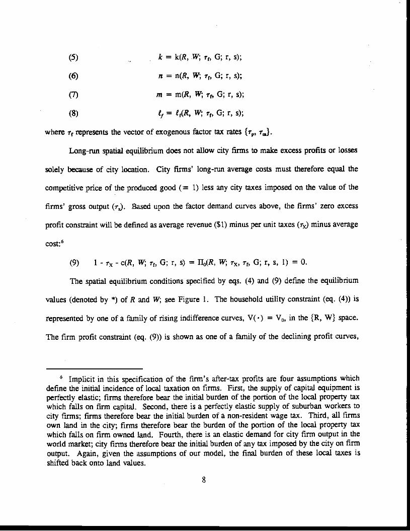
(5) k = k(R, .W; T, G; r, s);
(6) n=n(R,W;r,G;r,s);
(7) ,n=m(R,W;r,G;r,s);
(8) 4 = t4R, W; r, G; r, s);
where Ic represents the vector of exogenous Ittor tax rates {r, r,,j.
Long-nm spatial equilibrium does not allow city firms to make excess profits or losses
solely because of city location. City firms' long-run avenge costs must therefore equal the
competitive price of the produced good ( 1) less any city taxes imposed on the value of the
firms' gross output (rJ. Based upon the factor demand curves above, the firms' zero excess
profit constraint will be defined as avenge revenue (Si) minus per unit taxes (r,rJ minus average
cost:6
(9) 1 - Tx - c(R, W; r, G; r, s) = 110(R, W; Tx Tç, 0; r, s, 1) = 0.
The spatial equilibrium conditions specified by eqs. (4) and (9) define the equilibrium
values (denoted by *) of 2? and W; see Figure 1. The household utility constraint (eq. (4)) is
represented by one of a family of rising indifference curves, V(.) = V0, in the {R, W} space.
The firm profit constraint (eq. (9)) is shown as one of a family of the declining profit curves,
Implicit in this specification of the firm's after-tax profits are four assumptions whichdefine the initial incidence of local taxation on firms. First, the supply of capital equipment isperfectly elastic; firms therefore bear the initial burden of the portion of the local property taxwhich falls on firm capital. Second, there is a perfectly elastic supply of suburban workers tocity firms; firms therefore bear the initial burden of a non-resident wage tax. Third, all firmsown land in the city; firms therefore bear the burden of the portion of the local property taxwhich falls on firm owned land. Fourth, there is an elastic demand for city firm output in theworld market; city firms therefore bear the initial burden of any tax imposed by the city on firmoutput. Again, given the assumptions of our model, the final burden of these local taxes isshifted back onto land values.
8
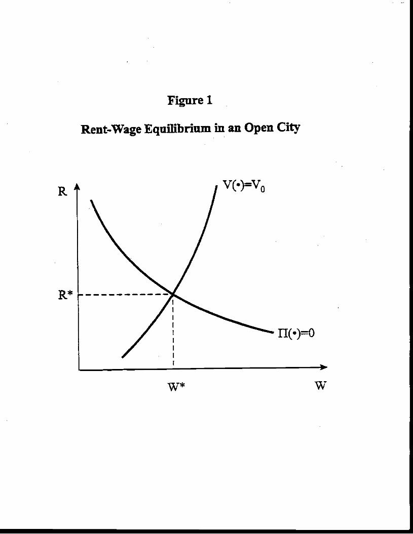
Figure 1
Rent-Wage Eqnilibrium in an Open City
fl(.=O
w* w
K4 V(•)=V0
= 0. Citizens will be better off if they can move to an indifference curve below V0
(earning higher wages andlor paying lower rents) and firms will be more profitable by moving
to a profit curve below fl(.) =0 (paying lower wages and rents). The equilibrium wage (W
and rent (R*) defined by the intersection of V0() and fl0(•) in Figure 1 are consistent with each
resident receiving V0 and each city firm receiving no excess profits or losses.
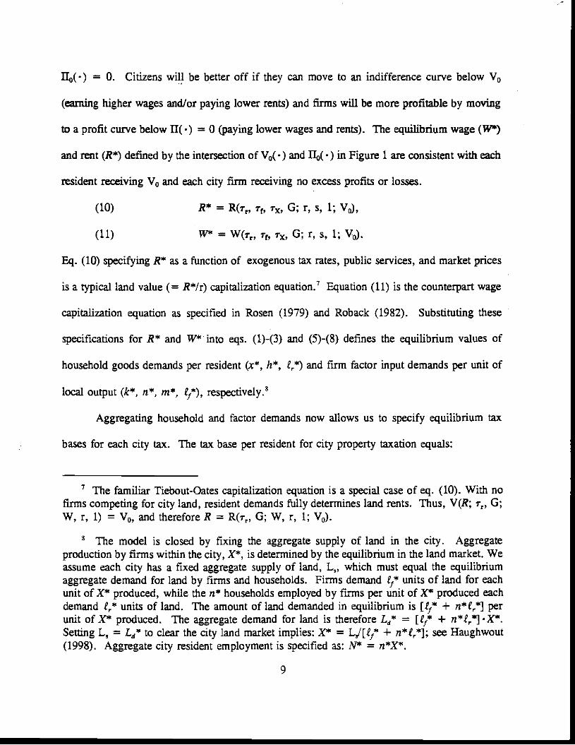
(10) R* = Rfr, T, T, G; r, s, 1; V0),
(11) = Wfr, r, r,, 0; r, s, 1; V0).
Eq. (10) specifying R* as a function of exogenous tax rates, public services, and market prices
is a typical land value (= Rfr) capitalization equation.7 Equation (11) is the counterpart wage
capitalization equation as specified in Rosen (1979) and Roback (1982). Substituting these
specifications for R* and WK into eqs. (i)-(3) and (5)-(8) defines the equilibrium values of
household goods demands per resident (x*, h*, 1r*) and firm factor input demands per unit of
local output (k*, n, m*, 17), respectively.3
Aggregating household and factor demands now allows us to specify equilibrium tax
bases for each city tax. The tax base per resident for city property taxation equals:
' The familiar Tiebout-Oates capitalization equation is a special case of eq. (10). With nofirms competing for city land, resident demands fully determines land rents. Thus, V(R; ;, 0;W, r, 1) = V0, and therefore R = R(r, 0; W, r, 1; V0).
The model is closed by fixing the aggregate supply of land in the city. Aggregateproduction by firms within the city, r, is determined by the equilibrium in the land market. Weassume each city has a fixed aggregate supply of land, L,, which must equal the equilibriumaggregate demand for land by firms and households. Firms demand units of land for eachunit of Xt produced, while the na" households employed by firms per unit of r produced eachdemand 4* units of land. The amount of land demanded in equilibrium is [17 + n*esc] perunit of X* produced. The aggregate demand for land is therefore Ld* = [17 + fl*Ir*] •r.Setting L, = Ld* to clear the city land market implies: X* = LJ[17 + n*lr*]; see Haughwout(1998). Aggregate city resident employment is specified as: N* = n*x*.
9

B,* = k*/n* + (R*/r)(tr* +. (t7/n)} + h,
(12) = 8iATr ?f, Tx, 0; r, s, 1, Va;
for city sales taxation:
B * =S
(13) B,5 = r1, T, 0; r, s, 1, Va;
for resident wage taxation:
= 1'1
(14) B* = B(r, Tç, Tx, 0; r, s, 1, Va;
for non-resident wage taxation:
=
(15) = Bm(Tr, T, 0; r, s, 1, V0);
and for local gross receipts taxation (remembering n' is resident-worker per unit of local
output):
Bx* = lIti,
(16) Bx* = t, r,, G; r, m, 1, V.
Though the model presented here is relatively simple, a priori predictions for the effects
on tax base of changes in tax rates and public good provision are generally not possible without
a parameterization of preferences and technologies. Fiscal policies which affect the
attractiveness of the city to both households and firms shift both the households' break-even
indifference curve and firms' zero profit curve in Figure 1, preventing a priori predictions for
R* and W*. Without knowing the changes in R5 and W, no a priori predictions are possible
10
for household consumption, factor utilization, and finally tax bases.9 Matters must ultimately
be resolved empirically.
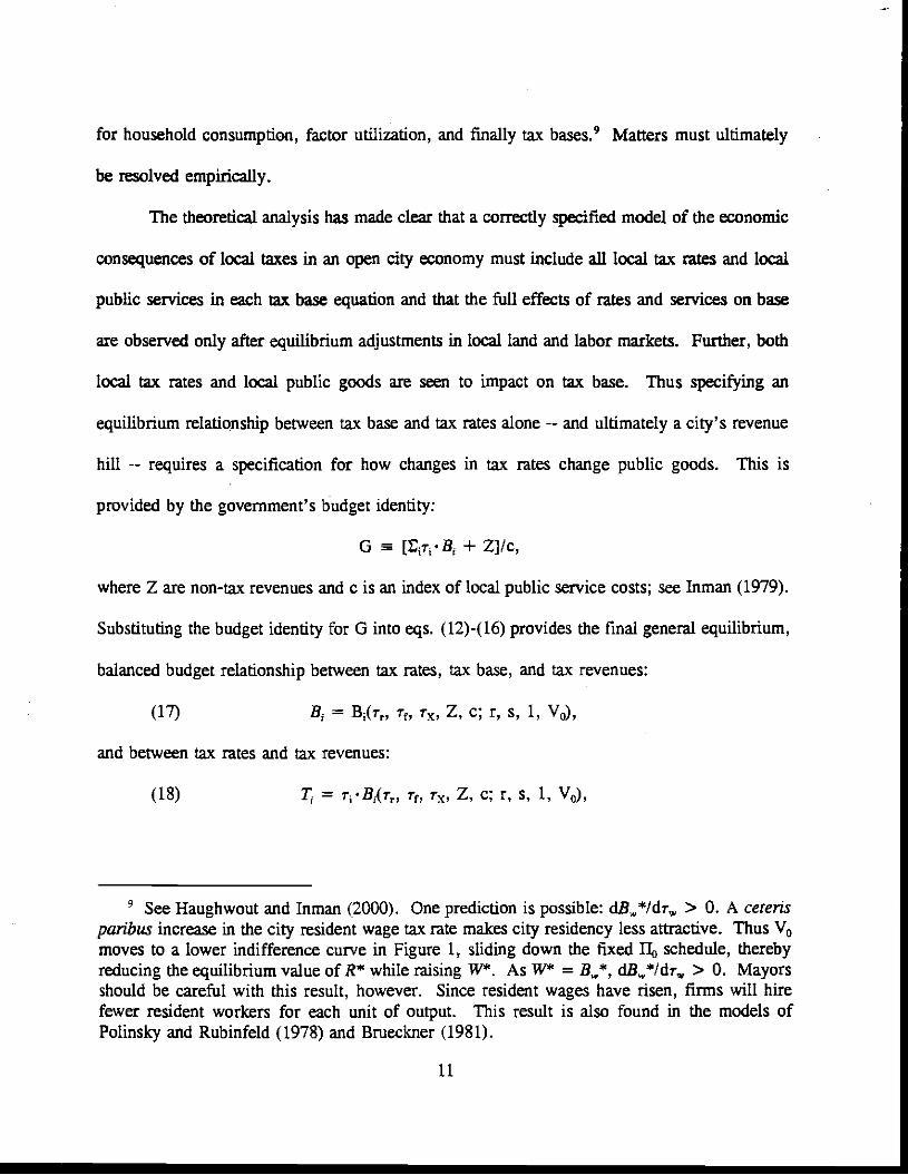
The theoretical analysis has made clear that a correctly specified model of the economic
consequences of local taxes in an open city economy must include all local tax rates and local
public services in each tax base equation and that the full effects of rates and services on base
are observed only after equilibrium adjustments in local land and labor markets. Further, both
local tax rates and lbcal public goods are seen to impact on tax base. Thus specifying an
equilibrium relationship between tax base and tax rates alone -- and ultimately a city's revenue
hill -- requires a specification for how changes in tax rates change public goods. This is
provided by the government's budget identity:
G [Er•B1 + Z]/c,
where Z are non-tax revenues and c is an index of local public service costs; see Inman (1979).
Substituting the budget identity for G into eqs. (12)-(16) provides the final general equilibrium,
balanced budget relationship between tax rates, tax base, and tax revenues:
(17) B1 = B(Tr, r1, Tx, Z, c; r, s, 1, V0),
and between tax rates and tax revenues:
(18) = rsB1('r, Ic, Tx, Z, c; r, s, 1, V0),
See Haughwout and Inman (2000). One prediction is possible: dB*Idr > 0. A ceteris
paribus increase in the city resident wage tax rate makes city residency less attractive. Thus V0moves to a lower indifference curve in Figure 1, sliding down the fixed ll schedule, therebyreducing the equilibrium value of R* while raising W*. As W* =B*, dB*/dr > 0. Mayorsshould be careful with this result, however. Since resident wages have risen, firms will hirefewer resident workers for each unit of output. This result is also found in the models ofPolinsky and Rubinfeld (1978) and Brueckner (1981).
11

for each local tax base [i= p, s, w, m, X].'°
The city's equilibrium revenue frontier is now defined as the aggregate of all city
revenues for each combination of city tax rates, specified as:
(19) 5.1? = trB,(r,, Tr' Tx, Z, c; •) + Z.
A small increase in any individual tax rate ( Mi), when coupled with adjustments in local
public goods as required by the city's budget identity, results in an equilibrium balanced budget
change in city revenues of:
(20) = Ar•B3 +
The first term measures the direct revenue effect of a small increase in the tax rate =
s, w, m, X). The second term measures the indirect effect of the rate increase as local tax bases
respond to changes in local tax rates and to balanced budget adjustments in G. The expression
within (} measures the change in each B1 because of the small change in ri; e11 is the elasticity
of B, with respect to changes in i. Since tax revenues are allocated to the purchase of public
goods, it is possible that the z's are positive -- for example, land taxes used to finance valued
public goods as in Brueckner (1982). For the general tax structures modeled here, however,
negative c's are also possible; see Haughwout and Inman (2000). Values of ed's are therefore
an empirical issue. We will estimate eq's for Houston, Minneapolis, New York, and
Philadelphia and use those estimates to place each city on its current revenue hill.
10Assuming, as we do, that the conditions for the Implicit Function Theorem hold for the
system of tax base equations plus the budget identity. Sufficient for a stable equilibriumspecification is that c > r1 3B,IdG, or in words, increasing G cannot bring in more in taxrevenues (Er1. 3B,/dG) than it costs to produce the good (c). This "reduced-form" approach tospecifying the equilibrium tax base equations is similar to that used by Vigdor (1998) in hisstudy of the property tax base for resident-only communities.
12

ifi. Data and Estimation
A. Data
The Data Appendix provides a summary of the data used in our analysis. All four cities
use a property tax (B,,, ri,); New York uses a general sales tax (B,, rJ;'1 New York uses an
income tax based upon the federal income tax definition of taxable income (B,,,, c,);'2 and
Philadelphia imposes a resident (B,,, r) and non-resident wage tax (B,,,, rJ and a gross receipts
tax (Br, rx). Unfortunately, Philadelphia data are not available to separate wage taxes collected
between residents and non-residents; we therefore estimate an avenge Philadelphia wage tax
base equation (B,,,j. For New York City and Philadelphia we also estimate a city employment
equation relating aggregate employment (N + Al) to local tax rates.
The property tax base per resident (B) in each city is the aggregate market value per
resident of all taxable property as estimated by each city from its tax roles using samples of
"arm's length" sales of properties within the city.'3 The sales tax base (Br) and the income tax
base (B,,) per resident for New York City are the City's estimates from tax returns of aggregate
retail sales and aggregate taxable wage and unearned (investment) income, respectively.
" Houston and Philadelphia also use a general sales tax, but there is insufficient variationin the sales tax rate over time to allow estimation of a revenue hill.
12 The wage tax base is approximately 75 percent of taxable income in New York City; seeTax Revenue Forecasting Documentation: Financial Plan, FY 1994-98, City of New York,Office of Management and Budget, 1994. New York City also imposes a non-resident incometax, but rates and revenues are low and rate variation is insufficient for empirical analysis.
' The estimates are not from (possibly biased) assessor's estimates, but from actual sales.Similarly, when specifying the effective tax rate on property in each city we use the estimatedratio of assessed value to market value (assessment rate) based upon market value as specifiedby market sales.
13
Philadelphia's gross receipts taxbase (B and wage tax base per resident (B,,, + B,,, =B÷J are
estimates from tax returns of aggregate business sales and of aggregate resident plus non-resident
wage income originating in Philadelphia. For New York City and Philadelphia, annual
aggregate employment (N ÷ Al) is also available as each city is also a county (ies for New
York); comparable data were not available for Houston and Minneapolis.
Each local tax rate, except for New York City's income tax, is a proportional tax rate.
For New York City's progressive income tax we define r as the top marginal rate; estimated
elasticities using the median income family's tax rate were similar. In all cities, property tax
rates (rn) are the effective avenge tax rate defined as the city's proportional mill rate times the
market value weighted avenge rate of property assessment within the city.'4 New York's
sales tax rate (r,) and Philadelphia's wage (r÷J'5 and gross receipts (ry) tax rates are the
statutory rates. There is significant variation in each city's tax rates, both up and down; see the
Data Appendix. All tax rate and tax base data were provided by either the city's Department
of Revenue or City Controller.
Other independent variables include: exogenous non-matching federal and state grants-in-
"Houston, Minneapolis, and New York City have different classes of property with
different effective tax rates for each class. For these cities we create a single tax-based weightedaverage of the separate property tax rates as our measure of ri,. The assessment to market valueratios are based upon market value as estimated from an annual sample of arm's length sales ofmarket properties.' The Philadelphia wage tax rate used to explain the aggregate resident plus non-residentwage tax base is a weighted average of the resident (r) and non-resident (r,,,) wage tax rates,specified as w+m = + .3. Tm where the weights were provided by the PhiladelphiaDepartment of Revenue, based on periodic Department surveys. We thank Mr. Michael Isardfor this data.
14
aid to the city (including school aid) minus net spending by the city on welfare (Z);16
exogenous determinants of the cost of local public goods (c) measured by changes in the national
industrial producer price index (1994 = $1.00); resident interest rates (r) measured by the AAA
corporate borrowing rate; non-resident wages (m) measured by national average hourly earnings
in nonagricultural industries; and the national rate of violent crime (CRIME) as a measure of
the relative attractiveness to residents of moving from the city to the suburbs (V0); see the Data
Appendix. (Unfortunately, continuous time series of city-specific crime rates were not available
for our four cities.) The relatively short sample periods in our study preclude us from including
all these exogenous variables in each tax base equation. As an alternative we will therefore use
two aggregate proxies for the time series patterns in these variables -- a simple time trend
(TIME) and the national rate of unemployment for civilian workers (UE) --and then include
each of the exogenous variables individually for separate analysis.
Also included in each tax base equation are measures of possibly important exogenous
economic or policy "shocks" specific to each city's economy. For Houston's property tax base
equation we test for the impact of the annual rate of change in crude oil prices (LFUEL). For
Minneapolis we test for the effects of seven years (1982-1988) of exogenous state funding for
downtown city construction, including a convention center and a new sports stadium
(STADIUM). For New York City we include the annual change in the inflation-adjusted Dow
Jones industrial avenge (ADOW) in each tax base equation. For Philadelphia we test for the
effects of changes in the national level of health care expenditures (AHEALTH) on tax bases.
Since the mobile middle class and firms determine land values and wages within the city,we use only exogenous aid which can be allocated to middle class and/or business services.Thus city welfare spending is subtracted from total exogenous grants-in-aid.
15

Both New York City and Philadelphia tax bases also may have been affected by policy "shocks"
from neighboring states, in particular, the introduction of the New Jersey state income tax in
1976 and, for New York City, the introduction of the Connecticut state income tax in 1991. We
include year indicator variables for the introduction of these taxes in the New York City and
Philadelphia base equations. Finally, beyond their decisions to set local tax rates, we test for
an independent effect of mayoral reputation on tax base by including indicator variables for the
nationally prominent mayors in our sample: Mayors Rizzo and Rendeil in Philadelphia, and
Mayors Koch, Dinkins, and Giuliani in New York City.
The tax base equations specified as eq. (17) are estimated here in first-differences to
allow for possible non-stationarity of the level time series in tax base and tax rates.'7 A test
for the possibility of pooling our four sample cities to obtain more precise estimates of the
effects of tax rates on the property tax base rejected pooling for these four cities.'8 All base
equations are therefore estimated separately for each city. Initial core equation estimates (Tables
1-3) are by OLS. Final equation estimates (Table 4) allow for the possible simultaneity of local
17 If we hope to recover the underlying structural relationship between tax rates and tax basefrom time series data, it is essential that all variables in the underlying relationship be generatedby stationary stochastic processes. Augmented Dickey-fuller tests (available upon request) revealeach of our national and city time series are first-order integrated processes 1(1). Given theseresults, all equations will be estimated in first differences. ADF test statistics for the residualsfrom the estimated core equations and the corresponding MacKinnon (1991) critical values areavailable upon request.
18 A pooled regression regressing iJ3,,, on a constant term, tSr,, tSUE, tSZ, and ISCRIMEhas an unadjusted R2 = .28. The pooled regression of SB on city-specific constants and eachvariable interacted with a city-specific indicator has an unadjusted R2 = .53. An F test for thesignificance of all interaction terms as a test of validity of pooling rejects the null hypothesis ofpooling at the .02 level of significance: F1574 = 2.507. Significant interactions were observedfor all tax rates.
16
tax rates and tax base. Instruments for tax rates include exogenous regulatory and political
events likely to affect local tax rates but not directly influence city tax bases — e.g., local
political election cycles, state tax rates, state spending other than grants to cities, the political
composition of the state legislatures, the political party of the governor, and a variety of city
specific regulatory events. lv estimates are provided even for local tax rates set by the state
(New YorkCity sales and income tax rates) or requiring state approval (Philadelphia wage tax
rates) under th! assumption that approval by the state may also be sensitive to changes in local
tax bases.
B. Estimation: Core Results
Tables 1 and 2 present our core estimates of the effects of changes in city tax rates on
changes in city tax base as well as estimates of each city's short-run and longer-run elasticities
of base with respect to own tax rate (aJ. Longer-run elasticities are reported for specifications
including three lagged rate changes for property taxation and two lagged rate changes for sales
and income taxes; longer lag structures did not contribute significantly to the explanatory power
of the estimated equation. The F statistic for the joint contribution of three lagged rate changes
(F(r(-3)) for property taxation and of two lagged rate changes (F(ai-(-2)) for sales and income
taxation are reported in Tables 1 and 2, respectively. Also reported for each equation are the
Durbin-Watson test statistic for the null hypothesis of no first-order serial correlation; in no
instances do we reject the null hypothesis.
Table I presents our core estimates for the property tax base equation for each city,
specifying changes in the property tax base per resident (a.B) as a function of a constant term,
balanced budget changes in the city's effective property tax rate (a), the national rate of
17

Table 1: Property Taxationt
houston Minneapolis New York Philadelphia
AD,, All,, All,, All,, All,, All,, AD,, AD,, All,, AR,, AD,, AR,,
Constant 7216 76.26 186.8 373.2 392.4 381.2 110.2 —14.97 59.94 123.3 102.0 89.7
(705.0) (7S1.9) (1000.0) (235.7) (247.4) (244.8) (332.2) (369.3) (341.7) (134.9) (157,9) (158.8)
AT,, —14,203.i —2,524.8k —1,205.9 10,673.0* —10,130.8 —3,0218 _3,091.7*
(5,891.7) (6,491.4) (8163.3) (896.9) (951.0) (1,246.8) (1,517.9) (1,663.2) (1,793.7) (603.9) (625.9) (721.9)
Aie(1) •-- 2,634.7(7,406.3)
—2,115.3(1,279.9)
—1,121.7(2,023.2)
— —123.4
(807;6)
Ai-,,(—-2)-— --- 9,076.5
(6,869.9)
— —1,261.2
(1,091.5)
—-- — 926.2
(2,121.7)
— — —1,257.8(767.9)
Ar,,(—3) -- —— 302.9
(6,610.7)
— —— —1,170.2
(954.4)
—
.
-— —2,709.7
(1,906.6)
— — —1,288.7(71L2)
AUE — —2.56
(664.3)
426.3
(761.8)
267.2
(252.4)
—122.7
(354.5)
303.4
(368.5)
314.8
(365.5)—174.6
(140.6)
—176.5
(147.3)
AZ —- 38.81
(35.89)
39.09
(41.92)
3.22
(2.21)
1.19
(2.28)
— 1.09
(1.57)
.35
(1.68)
— .75
(1.88)
—.08
(2.32)
AC'RlME -- 41.48
(27.50)
—- — —43(7.61)
— —— 5.59
(12.12)
— . — 3.44
(4.79)
—
D.W. 1.32 1.45 L52 1.50 1.31 2.15 1.12 1.43 1.24 1.40 1.65 1.72
A2 0.17 0.19 0.06 0,20 0.18 0.32 0.62 0.61 0.61 0.48 0.47 0.50
CUr —.40 —.28 ._.32* —1.11$
(.39) (.43) (.93) (.11) (.12) (.26) (.13) (.14) (.18) (.08) (.08) (.24)
F(Ar(—3))-— .59 -— 2.36* — .84 —— 1.58
Standard en'ois lot cacti estimated coellicieot are reported iii parentheses. D.W. is the Diirhiii-WaLson test statistic for serial correlation. ft2 is the coefliuent ofdetermination corrected for degrees of freedom. 'the elasticity of tax base with respect to tax rates (cur) is based on the marginal effects of rates on tax base,calculated for the immost recent Fiscal year's tax base amid tax tale for cacti city. F(AT(—3)) is time I" statistic testing time null hypothesis that three lagged changes inrates jointly have no iniloemice omm change in tax base.
*coelliciemmtls t statistic 2.00. Mnmmmeapohs' three lagged changes in rates are jointly signiFicant at the .10 level.
unemployment (zSUE), federal and state aid (including school aid) to the city net of welfare
spending (AZ), and the national rate of violent crime (ACRIME). The constant term provides
estimates of the average annual real growth in tax base. We test for the effects of changes in
public goods costs (Ac), interest rates (Ar), non-resident wages (Am), mayoral regimes, and
various economic shocks on these core estimates in Section ffl.C, Table 4 below.
For all four cities, Ar has a statistically significant negative effect on the rate of change
of the city's property tax base. In contrast, SUE, AZ, and ACRJME are not statistically
significant; a result confirmed in a pooled regression allowing for a common effect across all
four cities of AUE, AZ, and ACRIME on AB (available upon request). The insignificance of
AZ on city property values is consistent with the estimated negative impact of balanced budget
increases in property tax rates on property base. Both results imply additional public monies
are being allocated to uses not valued by property owners, for example, services for lower
income households or for public employee wage increases. City intergovernmental aid does
increase city revenues, but there are no important multiplier effects through an enhanced city
tax base. The insignificance of ACRIME on city property values may be due to the fact that we
are forced to use a national crime rate to proxy for local crime, though Cullen and Levitt (1996)
in their larger panel study of crime and cities found a similar insignificant effects of crime on
home values using city-wide crime rates. Other studies have found higher crime does reduce
home values, but only if it occurs in the home's immediate neighborhood; see Thaler (1978),
Hellman and Naroff (1979).
What matters most for changes in our sample cities' property tax bases are changes in
their tax rates. Table 1 reports the elasticities of each city's property tax base with respect to
18
changes in the city's property tax rate (EB,j, evaluated at the city's most recent year's tax base
and rate. The first two columns for each city in Table 1 provide estimates of the one-year,
impact elasticity of tax base with respect to changes in tax rates, measured as changes in the
market value of the city's tax base over the course of the fiscal year from a change in the city's
property tax rate announced before the beginning of the fiscal year. We also provide estimates
of a longer run tax base elasticity allowing for the effects of tax rate changes over the current
and three prior fiscal years.'9 These longer run elasticities are reported under each city's last
column in Table 1. The one-year impact elasticity is most likely measuring a capitalization
effect of rate changes on the market values of existing land and structures.2° The longer run
elasticity includes this capitalization effect as well as any effects of rate changes on firm and
household investments over the four year period, an adjustment period consistent with other
estimates of firm and household investment behaviors; see Caballero, Engel, and Haltiwanger
19 We have also estimated our model in levels specified as a stock adjustment model.Estimates of the underlying dynamic relationship between base and rates in the stock adjustmentspecification are consistent with the dynamic relationships estimated here; that is, newequilibrium values of tax base occur quickly, generally within four years. Results available uponrequest.
20 There may be some adjustments in firm and housing capital within the city over the initialfiscal year of the rate change. For example, as tax rates rise, firms may be able to relocate orsell existing capital not "bolted" to the plant floor. As tax rates fall, firms and households canundertake new investments in capital -- for example, expand the plant or add a family room.One would expect the one year response of physical capital to rate changes to be larger for ratereductions than for rate increases, given that it should be easier to expand firm and householdinvestment in place than to relocate plant and structures or to disinvest in housing; see Caballero,Engel, and Haltiwanger (1995) and Sinai (1997). To test this hypothesis, the impact elasticitieswere re-estimated allowing for asymmetric responses of the property base to rate increases anddecreases. In each city, the response to rate cuts was larger than the response to rate increases(as expected), but the differences were statistically significant only for Philadelphia. Fullestimates are available upon request, but see footnote 21 below.
19
(1995) and Sinai (1997). The impact elasticities are estimated precisely (t statistics generally �
3.00); the longer-nm elasticities are less well estimated and therefore should be interpreted with
care. With the exception of Houston, the estimated longer-run elasticities are larger in absolute
value than the estimated impact elasticities.
Both Houston and New York City show impact elasticities very close to, or possibly even
greater than, -1.0, the point at which the decline in tax base just offsets the added revenues from
the increase in tax rates. A balanced budget increase in the local property tax rate from current
levels will generate little or no additional net revenues for Houston or, barring large positive
effects on other bases (see Table 3), for New York City either. In contrast, Minneapolis and
Philadelphia with estimated impact elasticities for property taxation of -.3 and -.4 respectively
will be able to raise additional revenues from an increase in local property tax rates. These
initial revenue increases do not hold, however, as a rate increase erodes tax base over the next
three fiscal years. The longer run tax base elasticities for Minneapolis and Philadelphia are both
just over -.7, roughly twice as large as their impact elasticities and not statistically different from
-1.0.
Further, the significant negative impact elasticities, when interpreted in the light of the
structural model of Figure 1 imply that for the marginal property owners in our sample cities,
the property tax rate is too high. An increase in the city's property tax rate offset by a balanced
budget increase in public services may shift upward or downward the V0(•) = V0 indifference
curve for residents and the rI() = 0 breakeven line for firms. If improved services fail to
compensate households and firms for the rate increase, then V0() and fl0() shift downward.
Rents paid for land and structures in place and thus their capitalized values fall. Under an
20

assumption that the estimated impact elasticities of base with respect to balanced budget changes
in tax rates reflect a change in the capitalized values of land and structures in place --that is,
new investment or dis-investment in structures (h) and capital (k) take more than one fiscal year
to implement -- then the observed negative elasticities must mean the extra services provided do
not compensate either households or firms, or both, for the rate increase. The estimated impact
effects in fact allow us to compute the benefit shortfall. Houston, Minneapolis, and Philadelphia
property owners are estimated to receive about $.70 in additional benefits for each $1 in
additional property taxes paid, while New York City property owners are estimated to receive
only 5.02 in additional benefits for each $1 in new property taxes paid.2' In our sample cities,
21 From eq. (12) above, the estimated effects of a balanced budget increase in the localproperty tax rate reflects a capitalization effect of the rate and service changes on market valuesand any adjustments over the initial fiscal year by firms and households in their holdings ofphysical capital (k) and structures (h). If firms and households do not change k and h theestimated effect measures only the capitalization effect. This is most likely to be the case forthe estimated impact effects and, assuming disinvestment takes more than one year, is probablybest estimated by impact effects for rate increases only; see footnote 20. We use the estimatesof the impact effect of tax rate increases in our calculations below.
To estimate the additional benefit for each additional dollar of property taxes paid, notethat the market value of fixed structures and land will be the discounted present value of marketrents -- specified here as MV = RJr. Market rents in turn can be approximated by rents paidfor• the "private' attributes of the property (Ru) plus the value of the public services provided atthe location less the property taxes paid on the property: R = + vG - T, where u is thewillingness to pay for G. Finally, assuming a simple linear technology for services U = tT,then R = + [t4 - 1]-T, and MV = (RIr) + ([v4 - lj•TIr). The expression [t4 - 1]represents the net benefit of a dollar of property taxation. For a small property tax rate changeof Sr applied to the city's current tax base of MV0, AT = Ar 'MV0. Market values willtherefore change by AMV = ([u4' - l]Ir) - AT or by ([u$ - l]/r)Ar• MV0. Thus AMV/Ar =([u4' - fir) MV0 and, finally, [vt - 1] = [AMY/MI 'r/MV0. Knowing MV0, r, and usingestimates of [AMV/Ar], we can compute [v+ - 1j and thus u4', the marginal benefit of anadditional dollar of property taxation. We assume r = 3.00 (r is measured as a percent in ourregressions), MV0 is set at the sample mean market value for each city, and [AMV/M} is setequal to the estimated impact effect on the city tax base of rate increases only. The estimatedimpact effect of a property tax rate on city property values (standard errors in parentheses) are:Houston, -5041 (7431).; Minneapolis, -3286 (1932); New York City, - 9224 (3542); and
21

new property taxation must be being spent on public services in low demand by the marginal
property owner or on transfers to non-property owners (e.g., current and retired public
employees or low income residents)!2
Table 2 provides estimates of the effects of own tax rates on tax base for sales taxation
(New York City), gross receipts taxation (Philadelphia), income taxation of residents (New York
City), and wage taxation of residents and non-residents (Philadelphia). Increases in both the
sales (rà and gross receipts (ix) taxes act to reduce their respective tax bases, and the effects
are statistically significant (t � 3.70). The estimated impact elasticities of base with respect to
own rates are about - .60 for New York and -.25 for Philadelphia. Inclusion of lag changes in
; and r were never statistically significant and their inclusion had no significant effect on the
estimated base elasticities. We conclude the full effect of a change in the gross receipts or the
sales tax rate will be felt during the first year of the rate change. The New York City sales tax
base fluctuates with swings in the national unemployment rate (e, = -.12) around a stable
level of real sales per resident (insignificant constant term). Changes in exogenous city aid (SZ)
Philadelphia, - 1627 (840). Upon substitution, we estimate vi' = .67 (s.e. = .48) for Houston,= .67 (s.e. = .19) for Minneapolis, uP = .02 (s.e. = .38) for New York City, and ut =
.70 (s. e. = .15) for Philadelphia. Either u < 1 and avenge property owner values the servicesreceived at less than $1, or i' c 1 and the full tax dollar is not allocated to valued services, orboth.
Vigdor (1998) obtains similar empirical results for his sample of Massachusetts suburbancommunities and reaches a similar qualitative conclusion. Given his large cross-section ofcommunities Vigdor then tests for the likely sources of local rent-seeking. He concludes thatfor his sample of largely suburban communities the most plausible explanation for the negativeeffect of balanced budget rate increases is a fiscal redistribution from the avenge to lowervalued (median) property owners. For a sample of largely suburban communities, this seems areasonable result. In our sample of large cities, rent-seeking by public employee unions(Gyourko and Tracy, 1989) or poverty households (Glaeser and Kahn, 1999) are likely to playan important role too.
I4-

Table 2: Sales, Gross Receipts, and Tncoine Taxationt
SalesNew York
Gtoss ReceiptsPhiladelphia New York
lncozne/ Wage• Philadelphia
AB Aft, Aft, ABA- AB ABx ABw AD,,, AD,,, AB÷211 ABw+r,i AJJ+,,,
Constant 8015(80.59)
25.94
(91+70)
53.19
(88.17)
132+9
(224.4)
472.2
(263.2)
338.5
(211.9)
387.9
(218.4)
447.5
(231.1)
360.7
(218.4)
112.8
(70.30)71.42
(69.46)
66.46
(74.56)
Ar,,; Ar,,,÷,,, ---- —- -.
--— — 2,658.9(560.9)
—2,433.5
(581.9)—2,602.6
(546.1)—.198.3 .
(253,1)
—166.7
(215.6)
—402.0
(302.8)
Arw(—4);Arw±m(—1)— 1)034.6
(535.8)
— — 230.6
(223.7)
Ar,J-—2); Ar±,(—2) —— — —711.7
(567.1)
— — —23.62
(221.6)
Ar,,; Aix(251.7)
—1,137.4w(272.8)
—1,236.7(289.3)
—19,477.1(5,207.0)
—19,955.5k(5,083.4) (5,127.7)
— —
Ar,(—1);Arx(---1) - 141.8
(275.3)
3,796.5(5,197.2)
—
A-r,,(—2); Arx(—2) — --— —228.4
(265.6)
— 3,332.5(4,942.4)
— - — — — —
AUE —— ---158.5
(94.2)
—144.7
(95+7)
—- —293.1
(230.1)
—286.8
(208.7)
—--
—251.5
(232.0)
—347.3
(222.7)
——152.9
(58.21) (62.96)
AZ --- 39
(.41)
49
(.44)
-— —4.45
(2.95)
—1.98
(2.57)
— .14
(1.02)
.15
(1.01)
— .79
(.76)
.40
(.70)
ACRIME --- is(291)
— —- —14.09
(7.58)
-—- ---- —7.64
(6.98)
— — —.32
(1.99)
—
D.W. 2.18 2.14 1.91 1.88 1.50 1.84 - 2.71 2.63 2.84 1.21 1.35 1.36
A2 0.39 0.41 (1.40 0.30 0.48 0.54 0.46 0.46 0.53 0.01 0.18 0.23
ej,- —.61k
(.12)
,55#(.13)
..63*(.24)
—.25(.07)
—.25k
(.06)—.22
(.14)
—.84k
(.18)77(.18)
—.72(.31)
—.06
(.07)—.05
(.06)
—.06
(.13)
k'(Ai-(—2)) —- —— .40 — .26 — 2.69k — .41
Standard errors for each estimated codilicient are reported in parentheses. 111W. is the DurbiiiWatson test statistic for serial correlation. ft2 is the coefficient of determination correctedbr degrees of freedoti'. The elasticity of tax base with respect to tax rates (s,r) is based on the marginal effects of rates ott tax base, calculated for the most recent fiscal year's taxbase and tax rate for cacti city. b'(S-r(—2)) is the I" statistic testing the nell hypothesis that two lagged changes in rates jointly have ito iniluence on change in tax base.
4Coelhicicnt's t statistic � 2.00. New York City's two lagged changes in rates are jointly signiheant at the .10 leveL
L
and the national rate of violent crimes (ACRIME) have no important effects on New York sales
tax base. Philadelphia's gross receipts tax base is also sensitive to swings in the national rate
of unemployment = -.11); here the level of the base shows an upward annual trend
(constant term) avenging about 2.7% per annum (.027 = $472/$17,707). The Philadelphia
gross receipts tax base is affected by the upward trend in the national rate of violent crime; the
estimated elasticity is -.46.
New York City's income tax base per resident is sensitive to changes in the city's income
tax rates; the estimated impact elasticity of base with respect to changes in the top marginal tax
rate is statistically significant and important: e = -.84. The longer-run elasticity is smaller
(- . 72) but not statistically different from the impact elasticity; IV estimates reported in Table
4 show an important effect for lagged rates, however. The city's income tax base has been
growing at an avenge annual real rate of 3.46% to 4.29% over our sample period (.0346 =
$360.6/$10,420 to .0429 = $447.5/S10,420 ). Recessionary periods (e = -.18) and the
upward trend in the national rate of violent crime = - .40) have potentially important
negative effects on the city's income tax base.
In contrast to New York, Philadelphia's wage tax base per resident shows little overall
sensitivity to changes in the city's weighted average wage tax rate on residents and non-
residents. The estimated effect of changes in rate on base is small, = -.06, and statistically
insignificant. Nor has there been any significant growth over our sample period in the city's
real wage tax base per resident, again measured here by the magnitude and statistical
significance of the constant term. What does matter for Philadelphia's wage tax base are swings
in the national rate of unemployment (UE) = -.08). The small and insignificant base
23

elasticity for the Philadelphia wage tax should not lead to the conclusion that wage tax is without
economic consequences. On the contrary, the small base elasticity is the result of two very
important but offsetting real-side economic effects. We find below (Table 5) that the city's wage
tax drives out jobs and residents in roughly the same proportions, leaving the wage tax base per
resident about constant. As an economic and residential center, however, the city is significantly
smaller.
Table 3 reports own and cross tax-rate impact (one fiscal year) elasticities for New York
City and Philadelphia, based upon a first difference specification including all local tax rates,
a constant term, SUE, and zSZ. Only the tax rate elasticities are reported in Table 3.
Estimation is by Zellner's SUR procedure, equivalent to OLS in this case. Own impact
elasticities from these fully specified regressions are similar in magnitude and statistical
significance to those reported in Tables 1 and 2. The estimated cross-elasticities are generally
small, negative, and statistically insignificant. The one potentially important exception to this
pattern are the estimated positive (and almost statistically significant) effects of increases in New
York City's income tax rate and the Philadelphia's wage tax rate on each city's property tax
base. Figure I helps us understand why this might be so. Since residents bear the initial burden
of the resident income and wage tax and both residents and businesses benefit from the provision
of public goods, V0(.) is likely to shift downward while [L(-) rises. If, in Figure 1, V0() is
steeply sloped, then the upward shift in r10(.) can be sufficient to overcome the fall in V0() so
that the overall city rents (R*) and market values rise. V0(•) will be steeply sloped when city
residents strongly value other goods over living space, what we might expect for city
24
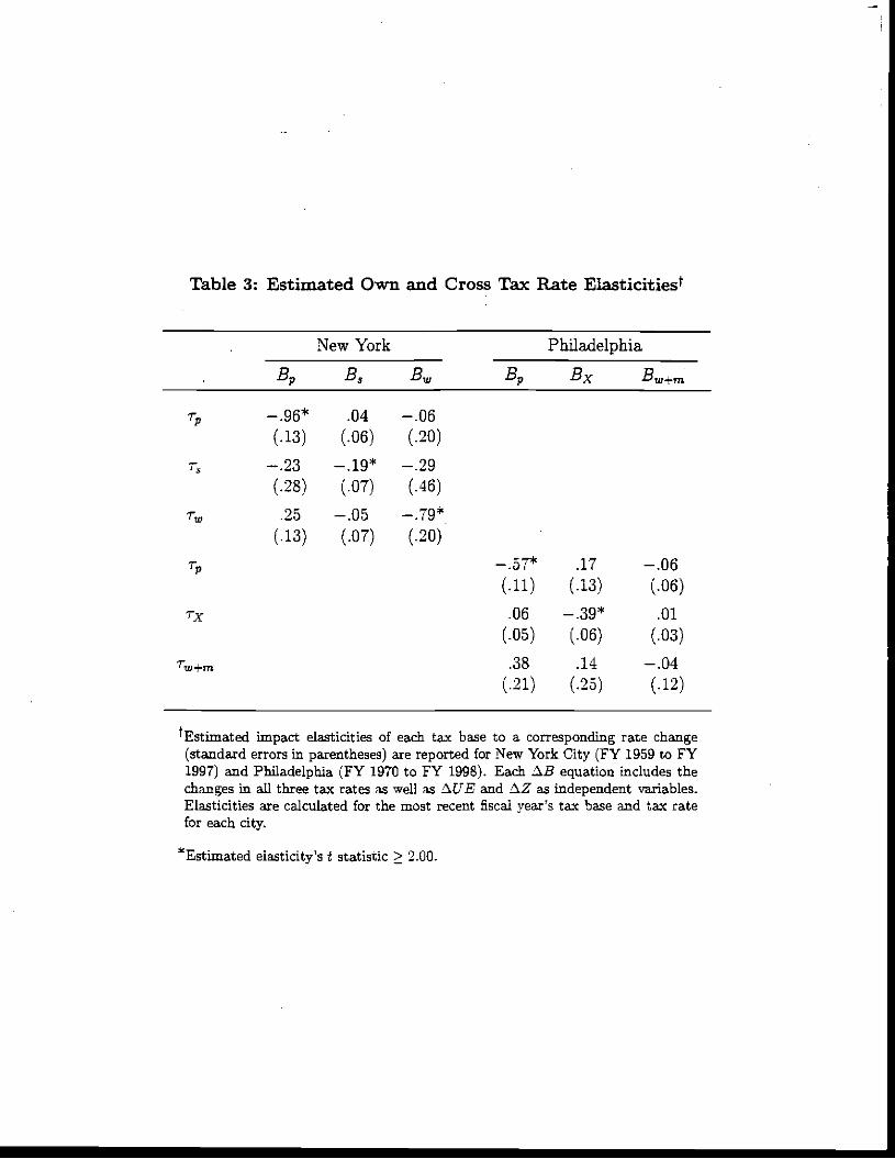
Table 3: Estimated Own and Cross Tax Rate Elasticities
.
.
New York Philadelphia
Ep B3 Bus By, B 2w+m
i-,,
(.13)
.04
(.06)
—.06
(.20)
r, —.23
(.28)
.19"(.07)
—.29
(.46)
r,, .25
(.13)
—.05
(.07)
79*
(.20)
7-y,
(.11)
.17
(.13)
—.06
(.06)
Tx .06
(.05)
.39*(.06)
.01
(.03)
w+m .38
(.21)
.14
(.25)
—.04
(.12)
tEstimated impact elasticities of each tax base to a corresponding rate change(standard errors in parentheses) are reported for New York City (FY 1959 to FY1997) and Philadelphia (FY 1970 to FY 1998). Each AR equation includes thechanges in all three tax rates as well as AUE and AZ as independent variables.Elasticities are calculated for the most recent fiscal year's tax base and tax ratefor each city.
*Estimated elasticity's t statistic 2.00.
residents!3
C. Estimation: Robustness
Table 4 provides two checks of the robustness of our core results, first to the inclusion
of possibly important exogenous economic "shocks" which may affect both tax base and tax rates
and then, second, to the possible endogeneity of local tax rates. Failure to control for either
local economic shocks or for the endogeneity of local tax rates may bias our estimated
elasticities. Our analysis here uses iSB regressed against r, SUE, and zXZ as a core
specification, but then adds city specific "Shock" variables to control for possible omitted
variable bias. Appendix B provides the first-stage estimates of local tax rates for our IV
estimation; instruments include exogenous political and regulatory events likel' to influencelocal
tax rates but not local tax base, at least directly.24
For Houston, we measure local economic shocks by the change in a four-year moving
average of the annual refiners' real (1994) price per barrel of domestic crude oil (4FUEL),
reported in Table 4 as "Shocks". Increases in the four year price of crude oil increases
Haughwout and Inman (2000) explore this argument more completely and show formallythat for plausible paraineterizations of the city economy income tax rate increases can increasecity property values in equilibrium.
24 The formal model also specifies a roles for the costs of local public goods (c: measuredby changes in the national industrial producer price index), the interest rate faced by firms andhouseholds (r: measured by the AAA corporate borrowing rate) and the non-resident wage (m:measured by national avenge hourly earnings in non-agricultural industries). As additionalsensitivity tests, we did include zIc, iXr, and m in each of the core tax base equations of Tables1 and 2. In most instances they had their expected signs in the .B equations (- for zIc for allbases; - for zlr for the property base, ambiguous for sales and income; ambiguous for m in allbase equations), but the estimated effects were only significant for âc in the Philadelphiaproperty base equation (c = -.62) and zSm in the two income tax base equations (ewm = .95for New York and Ew+mm = .80 for Philadelphia). Full results are available upon request.
25
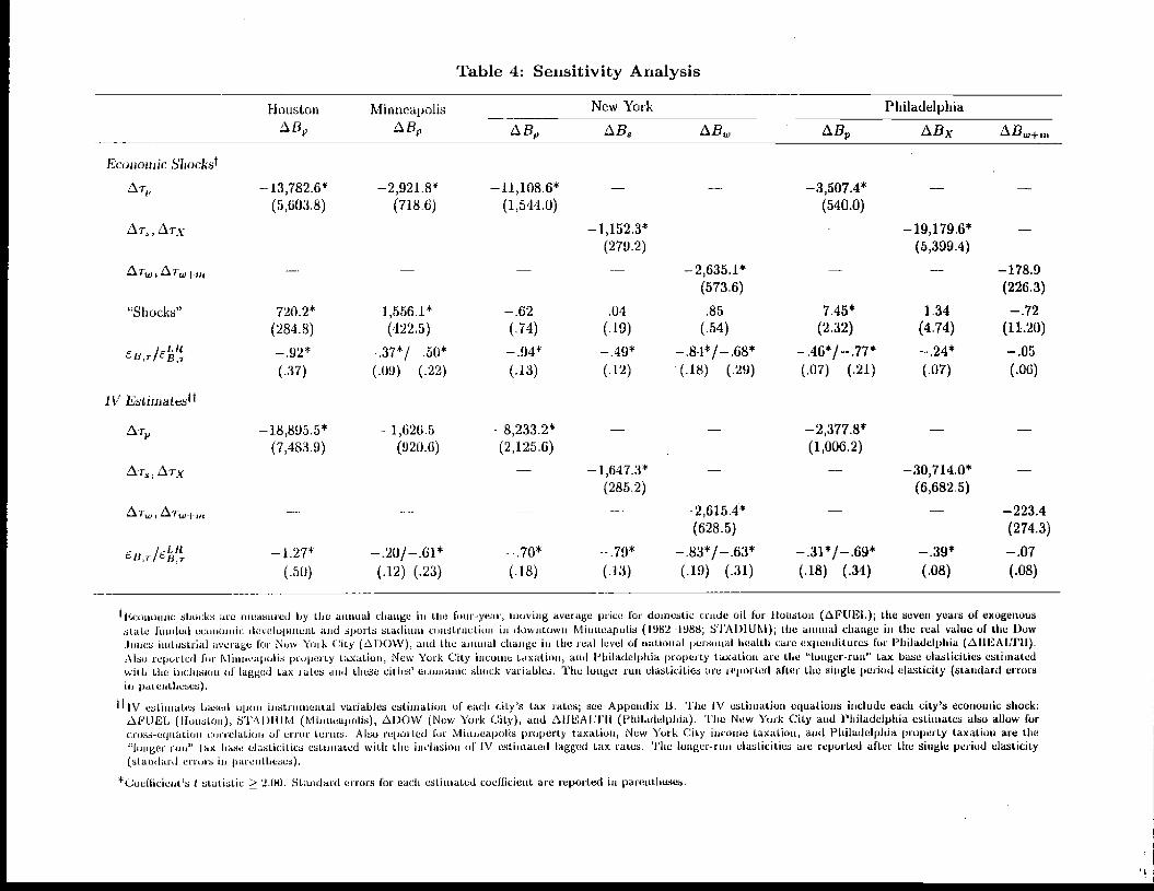
Table 4: Sensitivity Analysis
1-Inuston
ABMinneapolis New York Philadelphia
z\B AB5 AB ABx Bw-1-m
Economic Shockst
z;, —13,782.6(5,6(13,8) (718.6) (1544.0) (540.0)
L1T,TX --(279.2)
-(5,399.4)
L17w,L1w-1ni 2,635.1(573.6)
l78.9(226.3)
"Shocks" 720.2*(284.8)
1,5561k(422.5)
—.62
(.74).04
C19)
.85
(.54)7,45*
(2,32)1.34
(4.74)—.72
(11.20)
(37) (.00) (.22) (.13) (.12) (.18) (.29) (.07) (.21)
_.24*(.07)
—.05
(.06)
IV Esiinates1'
L1r —18,895.5
(7,4819)
—1,626.5
(920.6)
—8,233.2
(2,125.6)
—-
.
—2,377.8(1,006.2)
&r5,Tx - —
(285.2)
——
. (6,682.5)
Ar,i1r1.÷,,, --- — --- —2,615.4(628.5)
- —-- —223.4
(274.3)
Ej),/E(.50) (.12) (.23)
—.70
(.18)
79*(.13) (.19) (.31)
—.3P/—.69(.18) (.34) (.08)
—.07
(.08)
Ec,,iioiiiic shocks ale nieasuretl by the annual change in the foor—year, iloving average price for domestic crude oil for lleuston (AFLJEI); the seven years of exogenousstate Ion' led econio,, Ic tccelopioent and sports si-au inni coiustroctiou , ii, , lowotowo Miuiueapolis (1082 - 1088; S'I Al)! U NI } the aninual change iii the real value of the Dowliii Les mu usiriiul avc'i-age for N ow York City ( DOW), and the auuiuural change iii the lea! level of national personal IiealLli care expenditures for Pluiladelphis (J I EA If!'!!)A so reported for Minneapolis property taxation, New York City incoutue taxation, and Pluilarlelhuluia property taxation are the 'longer-run" tax base elasticities estuinatedwith the inclusion if lagged Lax u ales sri'! these cities' ecouuouoic slLock variables. The longer—run elasticities are reported after the single period elasticity (standard errorsiii parentheses).
IV esti ii ales basel upon iu,struuuiueotal variables estiuustion of each city's tax rates; see Appendix B. The IV estimation equations include eadu city's econonnc shock:M'lJEE (lloustoo), S'I'A l)IIJM (Minneapolis), M)OW (New York City), and llEAlJl'll (Philadelphia). Flue New York City and Pluiladelphia estimates also allow forcross—eq nation, c,iri-elstiuiuu of error terous. Also reported for M iuouoapolis property taxation, New York City incOme taxation, and Pluihuuielphiia property taxation are the"louigec—rnou" tax base elasticities estionated wiLl, the ir,closiou, of IV estimated lagged tax rates. 'flue longeu—rtni elasticities are reported after the single period elasticity
(staouhoil errors iii l' o theses).4Coellicieiut's I statistic ? 2(10. Standard errors for cad' estimated coetlicieuut are reported in parentheses.

Houston's property base wth an estimated elasticity of base with respect to FUEL of .24 (s.e.
= .09). With the inclusion of FUEL, the estimated elasticity of tax base with respect to tax
rate falls from -1.17 to -.92; compare Tables 1 and 4. To control for the potential endogeneity
of Houston's local property tax rate we re-estimated the core base equation using a predicted
value of local tax rates to estimate r; see Appendix B. Our instrumental variables (1V)
estimate of eB, for the core specification including AFUEL is -1.27 (s.e. = .50); see Table 4.
Overall, our OLS and IV estimates of e are all near, or exceed, -1, suggesting Houston is at,
or over, the top of its property tax revenue hill.
For Minneapolis, we included as our measure of a local economic shock an indicator
variable (STADIUM) equal to 1 for the seven years of state funded downtown economic
development, including the construction of the Hubert H. Humphrey Metrodome and the
Minneapolis Convention Center, 0 otherwise; see "Shocks" in Table 4. For each of those seven
years, the city's property tax base gained an avenge of $1556/resident for a total increase in
value of S 10,892/resident (= 7 x $1556). Interestingly, this estimated growth in property values
over this seven year period accounts for all the real growth in the city's tax base over our 24
year sample period; Minneapolis's property base would have been stagnant in real terms without
this state intervention. Including the indicator variable STADIUM has no significant effect on
the impact base-to-rate elasticity but it does reduce our estimate of the longer-run elasticity from
-.72 (Table 1) to -.50 (Table 4). The IV estimates for the Minneapolis property tax equation
(now including STADIUM) show some evidence of possible simultaneity bias as well; the impact
elasticity falls from -.37 (Table 4) to -.20 (Table 4). The longer-mn elasticity is not affected
by IV estimation.
26
For New York City, the annual change in the real (1994) value of the Dow-Jones
Industrial Avenge (DOW) was added to each of the core tax base equations to measure the
possible influence of the city's financial sector on tax base; see "Shockf in Table 4? SDOW
was marginally significant only in the city's income tax base equation (t = 1.57), where the
estimated elasticity of base with respect to the DOW is .18. Adding ADOW to the base
equations had no important effects on our estimated tax base elasticities; compare Tables 1 and
2 to Table 4. What does make a difference to our estimates of the city's base-to-rate elasticitiSs
is allowing for the potential endogeneity of local tax rates. The IV estimates (including SDOW)
are reported in Table 4. With IV estimation, the property tax base elasticity falls from -.94
(OLS; Table 4) to -.70 (IV; Table 4), while the sales tax base elasticity rises from -.49 (OLS;
Table 4) to -.79 (IV; Table 4). The impact and longer-run income tax base elasticity estimates
are robust to IV estimation, -.84 (OLS; Table 4) vs. -.83 (IV; Table 4) and - .68 (OLS; Table
4) vs. - .63 (IV; Table 4), respectively.
For Philadelphia, whose current economy is closely tied to the national health care sector,
we included the annual change in real (1994) national health care expenditures (SHEALTH) as
a measure of a local economic shock. The variable is statistically significant in the property tax
base equation only; see "Shocks" in Table 4. The elasticity of the city's property base with
respect to changes in national health spending is .63 (s.e. = .22). There are no important effects
We also included an indicator variable in income tax base equation called FedReformequal to 1 for the fiscal year after the passage of the 1986 Tax Reform Act. The 1986 federaltax reforms broadened the federal tax base and potentially the New York City income tax baseas well. The estimated coefficient for FedReform was 822.4 (s.e. = 1612.9) implying anincrease in base of about 8 percent. The inclusion of FedReform had no important effects onour estimates of e9 for income taxation.
27

of including &HEALTH on our estimates of Philadelphia's base-to-rate elasticities; compare
Tables 1 and 2 with Table 4. lv estimation (including £HEALTH) lowers the property tax
base elasticities both in the short run — from -.46 (OLS; Table 4) to -.31 (IV; Table 4) — and
the longer run -- from -.77 (OLS; Table 4) to -.69 (1V; Table 4), but the gross receipts tax base
elasticity rises from -.24 (OLS; Table 4) to -.39 (lv; Table 4). Wage tax base elasticity is
unaffected by IV estimation.
Two further sensitivity tests were performed. During our sample period both Connecticut
and New Jersey introduced personal income taxes for state residents, two 'policy shocks" with
possibly favorable effects on the tax bases for New York City and Philadelphia. We included
in each tax base equation an indicator variable equal to 1 for the year in which New Jersey
(1976) and (for New York City only) Connecticut (1991) introduced a personal income tax.
There were no significant effects of these out-of-state tax reforms on the income or sales tax
bases of either city. There were, however, statistically significant and economically important
effects on both cities' property tax bases, felt fully within the first year of the reform. The
reforms had no significant effects on the changes in the property tax base beyond the year of
their introductions, supporting an interpretation of these estimated effects as fiscal capitalization.
The introduction in New Jersey of a state income tax in 1976 raised New York City's property
values by $4989/resident in 1977 (s.e. = 1740), while the adoption by Connecticut of their
income tax in 1991 raised New York City property values in 1992 by $5347/resident (s.e. =
1796). The estimated coefficients imply the capitalization of from 22 percent (Connecticut
reform) to 38 percent (New Jersey reform) of the state income tax differentials into City
property values. The effect of the New Jersey income tax on the Philadelphia property tax base
28

is also statistically significant, increasing average city values by $2330/resident (s.e. = 1014).
The implied rate of capitalization of state tax differences into Philadelphia property values is 17
percent. The different rates of capitalization can most likely be attributed to differences in the
demand for land by businesses in the two city economies.Th For neither city did the inclusion
26 The introduction of a new tax on households (without compensating services) by the city'scompetitive political jurisdictions makes those jurisdictions less attractive. This raises V0 inFigure 1. For a given II, schedule, R* therefore rises. Thus new taxes in neighboringjurisdictions will be capitalized back into city values N R*Ir). For comparable upward shfitsin V0, the observed increases in R*/r allows us to identify the relative slope of the U schedule.A city with a business sector for which land is relatively (un)important in production will havea relatively (steep) flat fl schedule; see Haughwout and Inman (2000).
For New York City, the 1976 New Jersey income tax introduced a progressive tax onresident income with rates ranging from 1.5 to 3 percent. An avenge 1976 family consideringliving in New York or New Jersey had an annual income of approximately $40,000 per familyin 1994 dollars. This family's faced a new Jersey state income tax rate of approximately 3percent. They will therefore pay an additional $1200/year in taxes; this provides an incomeequivalent estimate of the maximal upward shift in V3. If the II schedule is very steep, R* willrise roughly $ 1200/year as well. Capitalizing this maximal increase in R* at a real interest rateof .03 per annum implies an maximal increase in the value of city land and structures of about$40,000 ( = $12001.03) per "parcel" or about $13,333/resident (assuming three residents perfamily). The estimated increase in value is $4989/resident following the introduction of the NewJersey income tax. Actual capitalization is therefore 37 percent of maximal capitalization. InFigure 1, the fl4 schedule for New York City must be "moderately" negatively sloped. Asimilar calculation for the introduction of the Connecticut income tax gives a similar result. The1991 Connecticut income tax rate was 1.5 percent but was understood to rise to 4 percent in1992. For a New York City or Connecticut family with the avenge income of $55,000 (1994dollars) we use the expected tax rate of 4 percent and an implied tax burden of $2200/year --again a rough estimate of the upward shift in V0. For a very steep [L0 schedule, the maximalincrease in R would therefore be $2200/year. Capitalized at .03 per annum implies an increasein value of city land and structures of $73,333 or $24,444/resident (assuming three residents perfamily). The estimated increase in value is $5347/resident following the introduction of theConnecticut income tax. In 1991 for the Connecticut income tax increase, the actualcapitalization is estimated to be 22 percent of maximal capitalization. Again we conclude 11e ismoderately negatively sloped, and perhaps flatter (land becoming more important in businessproduction) than it was in 1976.
For Philadelphia, we also assume a typical family choosing between Philadelphia andNew Jersey in 1976 had an annual family income equal to $40,000 in 1994 dollars. New NewJersey income taxes will again equal $1200 per year. Assume V3 rises by this amount. If H0 isvery steep, then maximal capitalization into rents (R*) will occur, and, as above, will equal
29
of these policy shocks have important effects of the estimated base-to--rate elasticities.
Our final sensitivity test adds to each tax base equation an indicator variable equal to 1
for the mayoral regimes of the nationally prominent mayors in our sample cities. Controlling
for the fiscal policies of the city and its core economic environment, does the national
prominence of a city's mayor enhance or hurt city tax bases? We tested this proposition
sequentially for Mayors Koch, Dinkins, and Giuliani of New York City and Mayors Rizzo and
Rendell of Philadelphia. For only one mayor was the mayoral indicator variable statistically
significant: Mayor Rizzo cost the Philadelphia wage tax base an avenge of -$282/resident per
year (s.e. = 122) over his eight years in office (about 2.1 percent of avenge city wages). With
this one exception, it has been the fiscal policies of the cities' mayors, not the mayor's
reputation, managerial style or personality, which has determined city tax bases.
D. Estimation: Taxes and City Jobs
As a further test of the underlying model and tax base specification, Table 5 provides
evidence of the effects of changes in city taxes, and associated public spending, on the one
dimension of the real economy we can measure with annual time series data: city jobs. The
Bureau of Labor Statistics' annual employment series are available by county. For New York
City (composed of five counties) and Philadelphia (a city-county) a time series of employment
corresponding to the city's political jurisdiction can be constructed. This is not possible for
Houston or Minneapolis. Results are presented for changes in each city's share of national total
$40,000 per parcel or $13,333/resident. For Philadelphia, the estimated increase in value is$2330/resident following the introduction of the New Jersey income tax. Thus actualcapitalization is 17 percent of maximal capitalization. We conclude that the ll schedule inPhiladelphia in 1976 is negatively sloped, and flatter (land more important) than was thecorresponding 1976 II schedule in New York City.
30

Table 5: Taxation and Job Location4
New York City (1970-1997) Philadelphia (1971—1998)
A Total A Total A Mann A Service A Total A Total A Mann A ServiceJob Skate Job Share Job Share Job Share Job Share Job Share Job Share Job Share
(OLS) (IV) (IV) (IV) —.00010
(.00048)
(OLS) (IV) (IV) (1V)
CoiistanL —.00076
(.01)043)
—.00077
(.0(1044) (.00(120)
— M0027t
(.00005)
OO023*(.00005) (.00006)
.00023*
(.00005)
Ar5; Ar5f10 — .00065*
(.00022)
.00070*(.00024)
0(11)8(3*
(.00028)
— .004)60*
(.00029) (.00011) (.00012)
— .00032*
(.00015).00032*(.00010)
Ar(—1); Ar5,.1.,J—1) JR)057*(.00021) (.00024) (.00028)
—.00047
(.00029)
.00031*(.00009) (.00011)
—.00036(.00015)
.00035*(.00011)
Ar(—2); Ar÷15j—2)(.1)1)019) (.00021) (.00027)
—.01)018
(.00025)
—.00009
(.0(1007)
m00025*(.00009) (.00012)
—.00016
(.00010)
AZ x 10_U
(.24 iu—)x 106
(.25 1o').26x 10_U
(.34 x i0—).lSx 10—6
(.30 < 10_6)
—:22 x 10_U
(.27 10_U)—.26x 10—6
(.28 x 10)—.SOx 10—6
(.38 x 1o_6)—.09x 10—6(.31 x
AlloW .26 x 10_U(.21 x t0)
.25 x 10(.21 x 10_U)
.31 x 10_U
(.25 x 10°).28 x 10_U
(.25 x 10_U)
AIIEALT1I —- - — - .78 x 10_U(.49 x 10)
.55 x 10—6
(.44 x jo_6).37 x io_
(.58 x 10_U).43 x 10
(.47 x 10—6)
13W. 1.25 1,33 1.74 1.22 1.83 1.91 1.74 2.01
fl2 .75 .74 .60 .68 .54 .60 .58 .40
EWM,r(.1)2) (.03) (.05) (.03)
_.12*(.06) (.06) (.11) (.06)
WfA:T,(.115) (.1)7)
4Q*
(.10)
—.14(.07) (.12) (.12) (.25)
45*
(.11)
F(A'r(—2)) 4.18* 4.18* 4.11* 1.50 4,fi5* 4.65* 2.47* 5.76
Stsiiilai-d eriota lii cciii eslittialed coefficient sic repoiI.ed in parentheses. D.W. is the i)urhin—Watson test statistic for setial coi'teiatioii. Whim approj)riitLC, estimationcorrected mi a first--order autoregressive noess 2 is the coeflicicut of tleteriiiiiiatuoii corrected for degrees of Ircedoin. 'L'iie elasticity of city jobs with respect tocilaiLgea iii the tIi iiiCLiLtiO or wage lax isle ci calculated for the lust year of thic flew tax rate as the "impact" elasticity (rN÷Ai,r ) and as the "bug—nut" elasticityalter tliiee Iisi:aI years iii the new tax rate (a ( AIr)• All elasticities are calculated at saLiLJule meals. 1"(ST(2)) is the I" statistic testing the null hypothesis that twolaggeil clL.LLL;L:a ill tOe have liii LolluitIlec 41 cliaiigtt iii job share; the teat was ciuiiiiuttsl ioi- liii) cirigitial OhS speeilicatiiiui.
*CiahliciilLLIa I -statistic -"'2.1)0. New York City's two lagged cilauLgea ii rates are jointly significant at .116 in the 'l'otal tool Manufacturing eqt1atiolls. I'1nladelphuias twoI agget I clot uiges iii r; tea a ic j uitit ly sig ii bean t at .05 ('l'o tab and Se rv ice) anti .1 0 (Maii u facto ii I ig)

employment, of national "manufacturing" employment (= manufacturing + construction +
communications + public utility + transportation employment), and of national "service"
employment (= FIRE ÷ retail + wholesale + services + federal and state government
employment). The constant term from each equation provides an estimate of the secular trend
in the each city's shaze of national jobs, holding fiscal policy constant. Changes in r and Z
measure the effects on jobs of tax and aid financed changes in public spending, respectively.
For each city, we estimated the effects of changes in each of the three local tax rates —property,
sales (New York) or gross receipts (Philadelphia), and income (New York) or wage
(Philadelphia) — on changes in city employment shares. Only changes in New York City's
income tax rate (measured as the top marginal rate) and Philadelphia's wage tax rate (measured
as the weighted average of resident and non-resident rates) showed statistically significant and
quantitatively important impacts on• city shares of national jobs7 These are the results
reported in Table 5, where we highlight the IV estimates. (See Appendix B for instruments.)
Income and wage tax rate changes longer than three fiscal years ago (current plus two lags) were
never statistically significant; F test statistics for the significance of two lagged rates based upon
the OLS estimates are reported for each specification in Table 5. Specifying city jobs as a share
of national jobs proved an adequate control for swings in the national economy; AIJE had no
important added effect on city job shares. ADOW and HEALTH are also included to measure
27 We tested for the effects of changes in each tax rate alone and jointly with changes in theincome or wage tax rates. While the effect of rate changes were generally negative on jobshares, only for the Philadelphia property tax rate in the, total employment and manufacturingemployment equations did the effect reach even marginal statistical significance (t = 1.4). Theimplied long-run elasticities of Philadelphia jobs with respect to changes in Philadelphia propertytax rates were -.20 for total jobs and -. 15 for manufacturing jobs. Results available uponrequest.
-
31

the effects on city job shares of. national shocks with possibly important local effects. Table 5
reports the implied impact (eN+Mj and longer-run (PN+M,) elasticities of jobs to current period
and to lagged changes in the city tax rates. For both New York City and Philadelphia local
taxes matte; for city jobs, particularly so for what we have classified as manufacturing jobs.
Our estimated elasticities for New York City and Philadelphia are consistent with results
obtained in other studies of the effects of taxes on jobs; see Bartik (1991; Appendik 2.2) for a
survey.
In 1970 New York City had 5.28 percent of the nation's jobs; today (1997) the city's
share is 2.81 percent. As demonstrated by the negative constant terms in each of New York
City's employment share equations there has been a steady secular trend away from city jobs,
with a greater rate of decline in the city's share of the national manufacturing as opposed to
service sector jobs. Compounding the secular loss in jobs share have been increases in the city's
income tax rates over the past thirty years, rising from a top marginal rate of 2.00 percent to
today's 4.46 percent. The OLS estimates in Table 5 show a statistically significant negative
effect of these rate increases on job share; the IV estimates are less precise but of comparable
magnitude. For New York City, the adverse effect of rising rates on city jobs is almost entirely
due to the negative impact of city taxes on the manufacturing sector; see Table 5. In contrast,
there appears to have been only a small adverse effect of city taxes on the city's share of
national service sector jobs; again, see Table 5. Of the total decline in New York City's share
of national jobs over the past three decades, approximately 16 percent of the decline can be
attributed to the rise in the city's income tax rates. This implies a loss of 492,000 city jobs from
32

1970 to 1997 because of increases in the city's income tax?
Philadelphia's share of national jobs has declined from 1.24 percent in 1971 to .54
percent by 1998. As in New York City, the negalive constant term in the share equations shows
a secular trend away from the Philadelphia economy, a trend affecting the manufacturing and
service sectors about equally. But also as in New York City, the rise in the city's labor tax rate,
here the weighted avenge wage tax rate, from 3.00percent in 1971 to a peak of 4.765 percent
in 1995 has been a major contributor to the fall in city jobs. Since 1996, the wage tax rate has
been reduced to its current (1998) avenge rate of 4.6025 percent. The OLS and IV estimates
of Table 5 both show statistically significant negative job effects of rising city wage tax rates;
the effects are felt in both the manufacturing and service sectors. Again, we can use the
estimates in Table 5 to allocate responsibility for the loss in city jobs. Of the total decline in
Philadelphia's share of national jobs over the sample period, approximately 21 percent of the
decline can be attributed to the secular rise in the city's wage tax rates. The estimated number
of city jobs lost because of tax rate increases over this period is 206,500. Mayor Rendell's tax
cuts begun in FY 1996 had restored approximately 11,800 jobs by the end of FY 1998.29
28 To calculate the contribution of New York City tax increases to the decline in the city'sshare of national jobs we first estimated the difference in the city's predicted job share withactual tax rate changes and the city's predicted job share with no tax nte changes. Thisdifference in job shares equals .40 percent, or about 16 percent of the actual decline in shares(= .401(5.28 - 2.81)). The total number of jobs lost over this period because of rising taxes isestimated as the change in job share due to tax increases times national jobs in 1997: 491,661= .004.122.915 million jobs.
29 To calculate the contribution of Philadelphia tax increases to the decline in the city'sshare of national jobs we first estimated the difference in the city's predicted job share withactual tax rate changes and the city's predicted job with no tax rate changes. For Philadelphia,this difference equals .15 percent, or about 21 percent of the actual decline in shares (=.15/(1.24 - .54)). The total number of jobs lost over this period because of the secular rise in
33

For both New York City and Philadelphia, Table 5 shows it has been the secular trend
against each city's economy coupled with rising city income or wage tax rates which explain a
significant fraction of the exodus of jobs from the city. There is nothing these two cities can
do about the secular trend, but balanced budget reductions in the city's tax rates can slow
decline, as has happened recently in Philadelphia. Of course, these rate reductions will cost city
tax revenues and, withoutefficiency gains, city services. The analysis here can provide estimates
of the revenue costs of each new job gained from cutting tax rates. Using 1997 values for
income tax revenues and total city jobs we estimate that for New York City the annual revenue
loss per new city job to be $2405/job per year or, since rate reductions must be permanent to
be credible, a present value cost $80, 167/job assuming a real discount rate of .03. Similar
estimates for permanent reductions in the Philadelphia's wage tax rate, evaluated at 1998 wage
tax revenues and rates imply anannual revenue cost per new city job of $2707/job per year or,
for a permanent tax cut, a present value cost of $90,229/job)° Tax cuts, while not sufficient
wage taxes is estimated as the estimated change in job share due to tax increases times nationaljobs in 1998: 194,719 = .0015. 129.813 million jobs. The Rendell tax cut is estimated to haverestored .009 percent to the Philadelphia job share or 11,775 jobs (= .009- 129.813 millionjobs) by 1998.
30 The marginal revenue costs of a new job can be estimated as .Revenue/aJobs, whereSRevenue = Revenues (1 + &8j . (M/'r) and where &Jobs = Jobs• N+M,r (r/r). Sincewe use the base-adjusted long-mn elasticities to estimate the effects of rate reductions onrevenues, the estimates of revenue costs will be net of the additional revenues made availableby the new jobs. Using New York City's 1997 values for income tax revenues (= $672/resident)and city jobs (= .47jobs/resident), and the IV estimates for E1flT (= -.63; Table 4) and 'N+M,r
- .22; Table 5), we estimate the annual revenue loss per new City job to be - $2405/job.The present value of these annual revenue costs will be equal to $80,167/job (= $2405/.03)assuming a 3 percent real rate of interest. Using Philadelphia's 1998 values for wage taxrevenues (=$723/resident) and city jobs (.46 jobs/resident) and the IV estimates for &Rs,r (= -.07; Table 4) and EN+M, (= -.54; Table 5), we estimate the annual revenue loss per new Cityjob to be -$2707/job. For Philadelphia, the present value of these annual costs will be equal to
34

by themselves to reverse the long-run secular trends against the New York and Philadelphia
economies — rates can only fall so far — will at leastslow the city's relative rate of economic
decline and provide increased employment opportunities for city residents. As a 'jobs
program" for inner city residents, however, the tax cut strategy appears more costly than
pwgrams which train and place residents directly in city or suburban jobs; see Heckman (1999).
Elected city officials must decide whether the private benefits of new city jobs are worth these
public costs of lower taxes and any resulting decline in city services.
IV. Revenue HIUs
Figure 2 presents estimates of each city's longer-run revenue hills for increases in city
tax rates from the city's current (last year of our sample) tax rate and revenue location. Each
city's revenue hills were simulated based upon the IV estimates including economic shocks
reported in Table 4•31 Four general conclusions emerge from the analysis in Figure 2.
$90,229/job (= $2707/.03).
31 Each revenue hill is estimated by the relationship Revenue = o B0 + Sr B0 + r0 SB+ SriSB, where To and B. are the actual tax rates and tax base for the last year of our sample,r is the change in tax rate from o to each new tax rate along the horizontal axis and SB is thepredicted equilibrium change in base for each Sr using the IV estimates reported in Table 4.For Minneapolis and Philadelphia property taxation and for New York City income taxation thelagged effects of changes in rate on base are included when estimating SB. (These IV pointestimates are not given in Table 4 but are available upon request.) Finally, to estimate NewYork City's income tax revenue hill, r0 and r are the tax rates for the avenge incomehousehold; however, SB is estimated from changes in the top marginal rate. We assume theavenge rate is linked to the top marginal rate through a simple proportional relationship,estimated from the thta in our sample. Consistent with our model specification, the topmarginal rates are reported on the horizontal axis of Figure 2, New York City, Income Tax.
35

Figure 2: City Revenue HiIIs*
600
400
200
0
Revenues1600 -
1400 —
1234
11631000
New York
800 —
600 —
400 —
200
0
Philadelphia
MinneapolisProperty Tax
H2.0 3.82 5.03 6.0
Revenue hills are based on estimated IV tax base elasticities as reported in Table 4. The solid lines between dots represent the portion of the bill which
spans the samole range for cay tax rates; the long dashed portions of each hiil are proectons beyond the samples range.
HoustonProperty Tax
Revenues
917905
800
/.4.
//I
N.4
1.0 2.0 '2.46 3.02.20
RevenuesProperty Tax
Tax Rate
Revenues
Sales Tax
Tax Rate
Income TaxRevenues
972.94
800
/600- I400- /
I
/1'
I
H
H
N '500
392r37
300-
2OO
.
/u1/ H// H
500469
400
300
200_/
0 I H' l__ioo-/
/1. I I I
//5.0 6.0 0 1 .0 2.0 3.0 4.0 6.0 TO 8.0
Tax Rate
/(
1.0 2.0 3.0 4.46 5.79 7.0Tax Rate
1.0 2.0 2.83 3.44Tax Rate
Property TaxRevenues
600 -
489
- / 1, N300- /I '
200 / I
100 Il
—
01' I
1.0 2.0 3.06 4.02.49 Tax Rate
200 -
100 -
0—
Revenues
1200 r
1000
600723
600
400
Wage Tax
.4-
Gross ReceEpts TaxRevenues
65 ,60-
40- I ,
30-/20- / I
10-/ 1
I 1 I I0
.1 .229 .4 .52.5 .7Tax Rate
//
/200
0
-//1
1.0 2.0 3.0 4.05.0 6.0 7.0 8.04.60 Tax Rate

First, with the exception of the Philadelphia wage and gross receipts tax, our sample
cities are very neas, or in the case of Houston's property tax over, the top of their local revenue
hills. The current (1997) Houston property tax rate is 2.46% and current revenues are
$905/resident; the revenue-maximizing rate, however, is 2.20% and maximal (1997) revenues
are $917/resident. Minneapolis is on the rising portion of its longer-run property tax revenue
hill, but the "summit" is fiat and available additional revenues are modest. Minneapolis' current
(1997) rate of 3.82% raises $.1163/resident while going to the maximal rate of 5.03% adds only
an additional $71/resident to $1234/resident. All three of New York City's taxes are now near
their maximal revenue potentials as well. The property tax can generate an additional
$3 1/resident (= $972/resident - $941/resident) by increasing the rate from its current (1997)
2.83% to 3.44%; the sales tax an additional $13/resident (= $392/resident - $379/resident) by
increasing its rate from 4.00% to 4.88%; and the income tax an additional $25/resident
($469/resident - $445/resident) by increasing its top bracket rate (and all other rates
proportionally) from 4.46% to 5.79%.
Philadelphia is the only city in our sample with an ability to raise significant additional
revenues per resident from local taxes, in this case from the local wage tax. Like our other
cities Philadelphia's property tax shows little new revenue potential; increasing its rate from the
current (1998) 2.49% to a maximal longer-mn rate of 3.06% will yield only $17/resident (
$489/resident - $472/resident) in new monies. The city's gross receipts tax is a small revenue
source generally and can raise only an additional $16/resident ($81/resident - $65/resident) from
increasing its rate from the current (1998) .29% to the maximal rate of .52%. As Figure 2
shows, however, the city's wage tax can generate significant new revenues per capita. But any
36

mayor adopting this strategy wins a Pyrrhic victory; raising the city's wage tax rate leads to
significantly fewer jobs (raffle 5) and most likely fewer residents as well. Both candidates
in the recent mayoral race in Philadelphia understood this point. An increase in the Philadelphia
wage tax rate now appears off limits politically because of its strong adverse effects on the size
of city's real economy.
Second, in both Minneapolis and Philadelphia we observe statistically significant and
quantitatively important differences between the one-year (impact) response and the longer-run
(equilibrium) response of the city's property tax bases to rate changes; the longer-run negative
response is larger. The peaks of the short-run property tax revenue hills (not shown in Figure
2) occur well beyond the peaks of Figure 2's longer-mn hills. The peak of the Minneapolis
short-run revenue hill occurs at a tax rate of 11.27% and maximal revenues are $2064/resident.
The peak of the Philadelphia short-run property tax revenue hill occurs at a rate 5.22% and
maximal revenues are $649/resident. For a mayor to aggressively pursue these short-run
32 A direct estimate of the effects of city taxes on city population is not possible since allannual population series available are unlikely to measure population variations with muchaccuracy. Still, simple arc elasticities between census years can be calculated to provide anorder of magnitude estimate for the effects of tax rates on population. Given the centralimportance of the wage tax to city jobs, we assume the wage tax is the most important taxdriving residents from Philadelphia. The simple arc elasticity of population with respect to theavenge wage tax rate is - .37 for the decade 1970 to 1980 and -.63 for the decade 1980 to 1990.A trend controlled estimate of the elasticity of city population with respect to wage tax rates canbe computed from the identity for the wage tax base (B w (N+M)/POP) and thecorresponding identity among elasticities: 8B. + €N+Mr - Our work provides trendcontrolled estimates of e (-.07; Table 4), Cwr (-.20; an IV estimate of the effect of rates on theavenge wage; available upon request), and tN+M. ( -.54; Table 5). These estimates imply8POPr = -.67. Both the simple arc elasticity estimates and the trend-controlled elasticity implya strong negative effect of wage taxes on city population for Philadelphia. This makes sensegiven that the only way to fully escape both the resident and non-resident portions of the tax isto move your job and your residence outside the city.
37

revenues may lead his city into the unproductive range of the longer-mn revenue hill, however;
see Inman (1989). It appears the current Minneapolis and Philadelphia mayors have avoided this
temptation, at least for now, keeping their cities on the rising portion of their property tax
revenue hills.
Third, while our cities are near the tops of their revenue hills,jumps in tax base will shift
the hills upward and provide additional revenues at stable rates. There are two possible sources
for base increases: annual tax base growth andfavorable economic shocks (FUEL, STADIUM,
SDOW, and AHEALTH > 0). The annual growth in city tax bases is estimated by the constant
terms in each ABASE equation; multiplying the growth in base by the revenue maximizing tax
rate provides an estimate of the maximal potential growth in annual revenues. For Houston the
(IV) estimated maximal growth in revenues is $8.95/resident per year (s.c. = 15.75); for
Minneapolis maximal revenue growth is $6.71/resident per year (s.e. = 14.80); for New York
City maximal aggregate revenue growth is $23.56/resident per year (s.e. = 12.10); and for
Philadelphia maximal revenue growth is -$3.52/resident per year (s.e. = 11.71), falling because
of the estimated annual decline in the city's property tax base.33 Annual growth in tax bases
is estimated to add at most 1.5% (for New York City) to aggregate city revenues.
If our sample cities are receive any revenue relief, it will have to come from
favorable, and generally large, shocks to each city's key economic sector.M For example, a
Calculations based on the estimated constant term for the IV estimates reported in Table4. Estimates and calculations available upon request.
All calculations here are based upon the IV estimates of each tax base equation, with eachcity's economic shock variable included. For Houston the estimated coefficient for 1FUELequals 732.0 (s.c. = 283.3) in the property base equation. For Minneapolis, the estimatedcoefficient for STADIUM equals 869.7 (s.c. = 566.6) in the property base equation. For New
38

one standard deviation increase in crude oil prices from the mean of $15.20/barrel to
$23.07/barrel (aFUEL = $7.87/baste!) adds $5760/resident to Houston's property tax base (=
SFUEL• ÔBASE/3FUEL = $7.87•732 (1V estimates)) and $127/resident to Houston revenues
using the city's revenue-maximizing tax rate (= .022 45760). For Houston, favorable oil
shocks are an important source of new city monies, here providing the city with an additional
14% in property tax revenues (= $127/$917). Of course, a one standard deviation decline in
oil prices will have an equally large but negative impact on Houston revenues. As noted earlier
Minneapolis's tax base benefited significantly from the seven years of state-funded downtown
construction (STADIUM), adding $10, 892/resident to the city's property tax base and potentially
$547/resident to city revenues evaluated at the maximal rate of .0503. Another construction
boom of this magnitude seems unlikely, however. The recent runup in the DOW has helped
New York City revenues, particularly income tax revenues. Our estimates suggest a one
standard deviation increase in the DOW of 1142 points will translate into an increase in New
York City's income tax base of $845/resident ( SDOW• olncomeBASE/aDOW = 1142 .74
(IV estimates)) for an annual 10 percent increase in city income tax revenues of $49/resident per
year when evaluated at the city's income tax revenue-maximizing rate (= .0579 4845).
Finally, Philadelphia revenues benefit from increases in national health care expenditures. A
one standard deviation increase in national health spending of $750/person is estimated to
increase Philadelphia's property tax base (the only significant effect) by $4470/resident (=
York City, the estimated coefficient for àDOW equals -.23 (s.e. = 1.04) in the property baseequation, -.05 (s.e. = .16) in the sales base equation, and .74 (s.e. = .56) in the income baseequation. For Philadelphia, the estimated coefficient for SHEALTH equals 5.96 (s.e. = 3.76)in the property base equation, -.14 (s.e. = 4.20) in the gross receipts base equation, and -.76(s.e. = 1.20) in the wage base equation.
39
AHEALTH 3PropertyBASEJÔHEALTH = $750 5.96 (IV estimates)) and the city's property
tax revenues by $137/resident evaluated at the estimated maximal rate (= .0306•4470), a 28%
jump in property tax revenues.
Fourth, no city should be at the top of its longer-nm revenue hill where the marginal
revenue from a small rate increase, and thus marginal public service benefits, are zero. Yet all
four of our cities are at, near, or even over the top, of their respective revenue hills.
Philadelphia wage taxation is the only exception. Why? Two answers suggest themselves.
First, when the dynamic structure of the local economy leads to a divergence of the short-run
and longer-run revenue hills, politicians seeking re-election in the short-run may not be able to
credibly promise to hold rates at a preferred longer-mn allocation; see Jnman (1989). In our
sample, however, the impact and longer-mn revenue hills diverge only for Minneapolis
(property) and Philadelphia (property), and even in these cities the longer-run effects are fully
felt within three to four years. Current voters are likely to bear, and therefore unlikely to
ignore, the negative effects on home values of short-term property tax rate increases. A second
explanation seems more promising — it may be simply that our cities' decisive voters want high
tax rates and a lot of public services. If so, evidence from our property tax base equations
(Table 1) suggest this decisive voter is not a value-maximizing homeowner. In our cities,
purchasers of city property place a negative net benefit on each marginal dollar of public
spending paid for through a dollar increase in property taxation; see Section IIll.B above. If
homeowners are not the decisive voters, who are? At least in Philadelphia, public employee
unions and residents of lower income neighborhoods are two likely candidates (Inrnan, 1995).
These two groups proved decisive in the recent mayoral victory of Democrat John Street, the
40

previous president of City Council who ran on a neighborhood spending platform. His
opponent, Republican Sam Katz made as his central campaign promises the expanded
contracting-oui of government services and the reduction in the city's wage tax rate from 4.6
to 4.0 percent. Street defeated Katz 51 %-49% largely because of the strong voter turnout and
support from the city's unions and lower-income neighborhoods.35 While local economics
determines a city's revenue hill, local politics determines where on that hill the city resides.
V. Conclusions
Understanding the equilibrium effects of local taxation on the local private economy is
important for elected city leaders, urban policy-makers, and academic economists alike. Our
analysis provides some important lessons for each group.
First, the mayors of each of our sanple cities are revenue constrained. Current tax rates
in Houston, Minneapolis, New York, and Philadelphia place each city very near the top of each
of its longer-run revenue hill(s). The Philadelphia wage tax is the one exception, but raising city
wage tax rates will cost the city jobs and residents. There is no obvious relief in sight. None
of our cities' tax bases show significant long-run growth. Favorable economic shocks have been
identified for each of our cities -- oil prices for Houston, downtown construction for
For a summary of the election see, the Philadelphia Inquirer, November 3, 1999. MayorStreet is now in office, and union contracts come due this summer. A recent article in thePhiladelphia Inquirer on the coming labor negotiations quotes the Mayor's inaugural address assaying: "We're going to work together. We're going to try to be fair in our relationships withthe unions and the great workforce of the city, and give them a quality of benefits that they areentitled and that we can afford." In addition, the Mayor's address promises $250 million forclean-up and physical improvements for the city's poorer neighbhorhoods. See the PhiladelphiaInquirer, January 25, 2000, p. R-1.
41
Minneapolis, a rising Dow for New York, and expanding health care spending for Philadelphia -
- but large upswings are needed for there to be any important revenue relief. Controlling local
expenditures seems essential for avoiding future fiscal crises.
Second, for New York City and Philadelphia, the two cities for which annual
employment data are available, we find city income and wage tax rates have important effects
on the location of jobs within the city. In New York City, a 10 percent increase in the city's
resident income tax leads to a 2.2 percent loss in total jobs and a 4.0 percent loss in
manufacturing jobs. In Philadelphia, the city's resident and non-resident wage tax has even
stronger negative effects. Here a 10 percent increase in the weighted avenge wage tax rate
leads to a 5.4 percent decline in total jobs and an 7.8 percent loss in manufacturing jobs.
Reducing these taxes will restore job opportunities to immobile, most likely poor, city residents
but at a likely cost of fewer city services. The estimated present value costs in lost revenues of
each city job created by a tax cut are $80,167/job in New York City and $90,229/job in
Philadelphia.
Third, when statistically significant, our longer-mn elasticities of base with respect to
rates, - .39 &L � - 1.27, generally exceed in absolute value the current estimates of the
elasticity of the U.S. federaj personal income tax base with respect to rates (= -.43, Gruber and
Saez, 1999) but are strikingly close to the elasticities obtained by Hines and Rice (1994) of -1.0
for small countries operating as international tax havens. Further, our estimated impact and
longer-run elasticities provide useful benchmarks for specifying Rosen-Roback style structural
models of fiscal policy in small open economies. The estimated impact effects on city property
values of changes in wage and income tax rates in New York and Philadelphia and in
42
neighboring Connecticut. and New Jersey are best understood using Figure 1 and a V0()
schedule which is rises steeply and a IT(•) schedule which falls modestly. V0(•) will be steep
when city households strongly value other goods more than living space, while fl(•) will be
weakly downward sloping when space, including vertical space, plays a relatively important role
in firm production.
Fourth, estimates of the city revenue hills provide the fiscal constraint necessary to
econometrically identify preferences of elected city officials. Our cities have all chosen to push
revenues to the top of their respective revenue hills. Why? The most likely explanation is a
political economy model which assigns a decisive role to voters with very high demands for
public dollars. The fact that property values fall as property rates increase suggest that in our
cities at least, these decisive voters are not value-maximizing homeowners.
43 -
REFERENCES
Amott, R. and J. MacKinnon (19Th, "The Effects of the Property Tax: A Genezal EquilibriumSimulation," Journal of Urban Economics, 4, pp. 389-407.
Auerbach, A. (1995), "Tax Projections and the Budget: Lessons from the 1980's," AmericanEconomic Review, Papers and Proceedings, 85, pp. 165-169.
Bartik, T. (1991), Who Benefits from State and Local Economic Development Policies?, UpjohnInstitute, Kalamazoo, MI.
Bound, I., D. A. Jaeger, and R. M. Baker (1995), "Problems with Instrumental VariablesEstimation When the Correlatioin Between Instruments and the Endogenous ExplantoryVariable is Weak," Journal of the American Statistical Association, 90, pp. 443-450.
Brueckner, J. (1981), "Labor Mobility and the Incidence of the Residential Property Tax,"Journal of Urban Economics, 10, pp. 173-182.
Brueckner, J. (1982), "A Test for Allocative Efficiency in the Local Public Sector," Journal ofPublic Economics, 19, pp. 311-31.
Caballero, R., E. Engel, and 3. Haltiwanger (1995), "Plant-Level Adjustment and AggregateInvestment Dynamics," Brookings Papers on Economic Activity: 2, pp. 1-39.
Cullen, J. and S. Levitt (1996), "Crime, Urban Flight, and Consequences for Cities," NBERW.P. No. 5737, Cambridge, MA: pp. 1-28.
Glaeser, E., H. Kallal, J. Scheinkman, A. Shleifer (1992), "Growth in Cities," Journal ofPolitical Economy, 100, pp. 1126-1152.
Glaeser, E. and M. Kahn (1999), "From John Lindsay to Rudy Giuliani: The Decline of theLocal Safety Net?" Federal Reserve Bank of New York: Economic Policy Review, 5, No.3, pp. 117-132.
Goolsbee, A. (1999), "In a World Without Borders: The Impact of Taxes on InternetCommerce," NBER WP. No. 6863, Cambridge, MA: pp. 1-29.
Grieson, R (1980), "Theoretical Analysis and Empirical Measurements of the Effects of thePhiladelphia Income Tax," Journal of Urban Economics, 8, pp. 123-138.
Grieson, R., W. Hamovitch, A. Levenson, and R. Morgenstern (1977), "The Effect of BusinessTaxation on the Location of Industry," Journal of Urban Economics, 4, pp. 170-185.
1

Gruber, I. and E. Saez (1999), "The Elasticity of Taxable Income: Evidence and Implications,"NBER Working Paper, pp. 1-32.
Gruenstein, 1. (1980), "Jobs in the City: Can Philazlelphia Afford to Raise Taxes," BusinessReview: Federal Reserve Bank of Philo4elphia, May/June, pp. 3-11.
Gyourko, J. and I. Tracy (1989),"Local Public Sector Rent-Seeking and Its Impact on LocalLand Values," Regional Science and Urban Economics, 19, pp. 493-516.
Haughwout, A. (1998), "Aggregate Production Functions, Interregional Equilibrium, and theMeasurement of Infrastructure Productivity," Journal of Urban Economics, 44, pp. 216-227.
Haughwout, A. and R. P. Inrnan (2000), "Fiscal Policy in an Open City Economy," WorkingPaper, Wharton School, University of Pennsylvania.
Heckman, J. (1999), "Policies to Foster Human Capital," NBER W.P. No. 7288.
Bellman, D. and I. Naroff (1979), "The Impact of Crime on Urban Residential PropertyValues," Urban Studies, 16, pp. 105-112.
Hines, I. and E. Rice (1994), "Fiscal Paradise: Foreign Tax Havesn and American Business,"Quarterly Journal of Economics, 109, pp. 149-182.
Hines, J, (1999), "Lessons from Behavioral Responses to International Taxation," National TaxJournal, 52, pp. 305-322.
Inman. R. (1979), "Dissecting the Urban Fiscal Crisis: Facts and Counterfacts," National TaxJournal, 32, 127-141.
Inman, R. (1989), "The Local Decision to Tax: Evidence from Large U.S. Cities," RegionalScience and Urban Economics, 19, pp. 455-491.
Inman, R. (1995), "How to Have a Fiscal Crisis: Lessons from Philadelphia," AmericanEconomic Review, Papers and Proceedings, 85, pp. 378-383.
Inman, R. and D. Rubinfeld (1997), "Rethinking Federalism," Journal of EconomicPerspectives, 11, pp. 43-64.
Mark, S., T. McGuire, and L. Papke (1998), "The Influence of Taxes on Employment andPopulation Growth: Evidence from the Washington D.C. Metropolitan Area," WorkingPaper.
2

MacKinnon, J. (1991), "Critical Values for Co-Integration Tests," in R. Engle and C. W. J.Gran get, Long-Run Economic Relationships: Readings in Co-Integration, OxfordUniversity Press, New York, pp. 267-276.
Polinsky, M. and D. Rubinfeld (1978), "The Long-run Effects of a Residential Property Tax andLocal Public Services," Journal of Urban Economics, 5, pp. 24 1-262.
Poterba, 1. (1996), "Retail Price Reactions to changes in State and Local Sales Taxes," NationalTax Journal, 49, pp. 165-176.
Roback, 1. (1982), "Wages, Rents, and the Quality of Life," Journal of Political Economy, 90,pp. 1257-1278.
Rosen, 5. (1979), "Wage-based Indexes and the Quality of Life," in P. Mieszkowski and M.Straszheim (eds.), Current issues in Urban Economics, Baltimore: Johns HopkinsUniversity Press, pp. 74-104.
Sinai, T. (1997), "Taxation, Mobility, and the Demand for Owner-Occupied Housing,"Unpublished Ph.D. Dissertation, MIT.
Staiger, D. and J. H. Stock (1997)., "Instrumental Variables Regression with Weak Instruments,"Econometrica, 65, pp. 557-585.
Sullivan, A. (1985), "The General Equilibrium Effects of the Residential Property Tax:Incidence and Excess Burden," Journal of Urban Economics, 18, pp. 235-250.
Thaler, R. (1978), "A Note on the Value of Crime Control: Evidence from the PropertyMarket," Journal of Urban Economics, 5, 137-145.
Vigdor, J. (1998), "Was Tiebout Wrong? Local Taxes and the Growth of Cities," WorkingPaper, Harvard University.
Walsh, M. and J. Jones (1988), "More Evidence on the "Border Tax" Effect: The Case of WestVirginia, 1979-1984," National Tar Journal, 41, pp. 261-266.
3
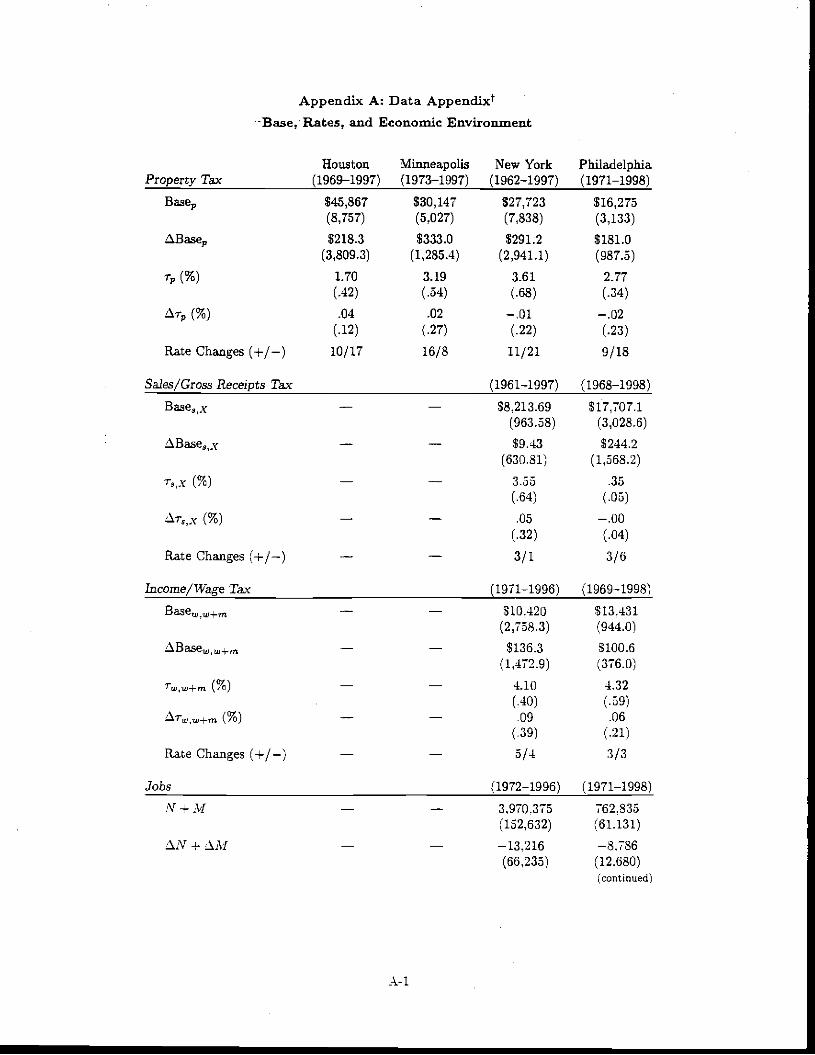
Appendix A: Data Appendix-Ease,Rates, and Economic Environment
Houston Minneapolis New York PhiladelphiaProperty Tax (1969—1997) (1973—1997) (1962—1997) (1971—1998)
Baser $45,867 $30,147 $27,723 $16,275(8,757) (5,027) (7,838) (3,133)
ABaseR $218.3 $333.0 $29 12 $181.0(3,809.3) (1,285.4) (2,941.1) (987.5)
r (%) 1.70 3.19 3.61 2.77(.42) (.54) (.68) (.34).04 .02 —01 —.02
(.12) (.27) (.22) (.23)
Rate Changes (+1—) 10/17 16/8 11/21 9/18
Sales/Gross Receipts lax (1961—1997) (1968—1998)
Base,,x $8,213.69 $17,707.1(963.58) (3,028.6)
ABase5,x $9.43 $244.2
(630.31) (1,568.2)
r (%) 3.55 .35
(.64) (.05)
ISr3,x (%) .05 — .00
(.32) (.04)
Rate Changes (+/—) 3/1 3/6
Income/Wage Tax (1971—1996) (1969—1998)
Basew,w+m $10,420 $13,431(2,758.3) (944.0)
$136.3 $100.6
(1,472.9) (376.0)
w,w+m (%) 4.10 4.32
(.40) (.59)STW,w+m (%) .09 .06
(.39) (.21)
Rate Changes (+1—) 5/4 3/3
Jobs (1972—1996) (1971—1998)
N + M 3,970.375 762.835(152,632) (61.131)
—13,216 —8.786
(66,235) (12.680)(continued)
A. I
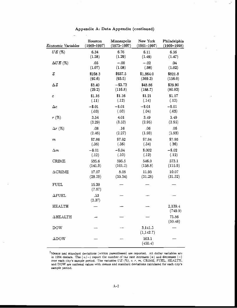
Appendix A: Data Appendix (continued)
Houston Minneapolis New York PhiladelphiaEconomic Variables (1969—1997) (1973—1997) (1961—1997) (1969—1998)
UE (%) 6.34 6.76 6.11 6.36(1.28) (1.29) (1.49) (1.47)
SUE(%) .05 —.00 —.02 .04(1.07) (1.08) (.98) (1.02)
Z $258.3 $937.5 $1,864.0 $821.8
(92.6) (93.5) (369.3) (156.0)
$3.40 —$3.72 $48.86 $29.90(29.2) (116.8) (188.7) (80.83)
c $1.16 $1.16 $1.21 $1.17(.11) (.12) (.14) (.12)
Sc .—$.01 —$.01 —8.01
(.03) (.03) (.04) (.03)
r (%) 3.54 4.01 3.49 3.49
(3.29) (3.52) (2.95) (2.95)
Sr (%) .08 .16 .06 .06
(2.46) (2.27) (1.93) (1.93)
in $7.86 $7.82 $7.84 $7.86
(.36) (.36) (.34) (.36)
—$01 —$04 $.002 —$.02
(.12) (.10) (.12) (.12)CRIME 535.6 595.5 546.0 573.1
(141.9) (101.2) (138.8) (115.9)
ACRIME 17.07 8.08 11.93 10.07
(28.29) (33.34) (31.28) (31.52)
FUEL 15.20
(7.87)
SFUEL .53
(2.37)HEALTH 2,139.4
(749.9)
SHEALTH 75.86
(50.48)
DOW 3,141.5(1,142.7)
SDOW 103.1
(450.4)
Means and standard deviations (within parentheses) are reported. All dollar variables arein 994 doilan. The (+1—) report the number of ta rate increases (-i-) and decreases (—)over each city's sample period. The variables UE (%), c, r, in, CRLME, FUEL, HEALTH,and DOW are national values with means and standard deviations calculated for each city'ssample period.
A-2

Appendix B: First Stage Estimates for Local Tax Rates
Table B summari2es the first stage estimates of city tax rates for each of our sample
cities. The Table provides the coefficient estimates for the excluded, predetermined variables
for each city. Also included in each equation as exogenous regressors (but not reported in Table
B) are a constant term, a time trend variable and the time trend squared, the national rate of
unemployment lagged one period, and each city's federal and state aid less welfare spending
lagged one period. The excluded pre-determined variables are meant to capture exogenous
determinants of local tax rates operating either through the local political process or through state
regulations of local government finances.
Local political variables include an election cycle indicator variable (Elect) equal to 1 for
the two years before a mayoral election and 0 otherwise (when Houston had a two year mayoral
term, Elect equaled 1 for the one year before the election), an indicator variable for Mayor
Dinkins (Dinkins, New York only) who ran on a progressive tax platform, and the percent of
the Philadelphia City Council who are racial minorities (%M1nCC, Philadelphia only) to
represent the significant shift in Council composition following the 1979 Abscam scandal.
Variables meant to capture the influence of the state regulatory environment on local finances
include the percent of state income collected as states taxes other than state income taxation
lagged one period (r(-l)), the percent of general state and local spending done directly by the
state (%SLExpS), the percent of the state lower chamber who are Democrats (%LegDem), an
indicator variable equal to I if the state's Governor is a Democrat (GovDem), and, for Houston
only, future annexation measured by city land area with a one year lead (Land(+ 1)), for New
B-i

York City only, the level of MAc bonds outstanding lagged one period (MACDebt(-1)), and for
Philadelphia only, an indicator variable for the 1977 borrowing crisis in which Wall Street
required tax rate increases to balance a deficit budget (CrisLi7Y) and the 1985 state-mandated
reformof the city's business taxes requiring a reduction in the city's gross receipts tax rate
(S5BflRef). When statistically significant or nearly so, each variable influenced local tax rates
in the expected direction: Elect (-), Dinkins (- in r, + in r,j, %MinCC (-), r,. (-), Land (-),
MACDebt (+), Crisis77 (+), and 8SBlJcRef (- in Tx, + or 0 for r and r,,..J. We are agnostic
as to the likely effects of %LegDezn and GovDem on city tax rates, holding constant state to city
aid (as our specification does). On the one hand, democratic state governments are likely to
increase local government mandates, particularly for services for the poor (+ coefficient as in
Minneapolis and New York City), but on the other hand, democratic states may wish to favor
democratic city administrations in ways not measured by grants-in-aid (e.g., providing more
state services within city boundaries, -coefficient as in Philadelphia). When significant, %SLErp
had a positive effect on Houston, Minneapolis, and New York property taxation, implying
cooperative, not competitive, fiscal federalism.
As a group the excluded predetermined variables are significant explanatory variables for
city tax rates. Though we cannot reject non-stationarity for the level series of tax rates and the
continuous value instruments in Table B, individually the variables are stationary in first
differences. Under the hypothesis that the system is 1(1), the Durbin-Watson test statistic for
the null hypothesis of non-stationarity of the residuals from the co-integrating regression is
appropriate (Engle and Granger, 1987). For each tax rate regression in Table B, the Durbin-
Watson test statistic allows us to• reject the null hypothesis of non-stationarity, or of no co-
B-2

integration, at the 1 percent level of significance (D.W. � .511; Engle and (hanger, 1987).
For completeness, the Augmented Dickey-Fuller test statistics for the stationarity of the error
terms of the co-intergrating regression assuming higher-order autoregressive processes are also
reported (MacKinnon, 1991). Our tax rate regressions pass this more demanding test in four
of our eight specifications. Assuming a stable, co-integrating regression, the predicted tax rates
using the level regressions from Table B are then used to compute predicted first differences in
rates for lv estimation reported in Table 4.
The quality of the predictive equation will determine the degree to which our instruments
successfully control for simultaneous equation bias. As recommended by Bound, Jaeger, and
Baker (1995) and Staiger and Stock (1997) we report the partial R2 and the F statistics for the
first-stage estimates. The partial R2's measuring the variation in local tax rates explained by the
instruments alone all exceed .32, and all but Minneapolis are .50 or larger. P-values based upon
an F test for the statistical significance for each group of excluded predetermined variables
uniformly rejects the null hypothesis of no influence of the selected instruments; see Table B.
For less than perfect instruments (i.e., instruments potentially correlated with the error terms
of the tax base equations), the inverse of the reported F statistic (1/F) is an approximate measure
of the finite sample bias of our IV estimates of the effects of rate on base relative to the OLS
estimates of the same coefficients; see Bound, Jaeger, and Baker (1995) and Staiger and Stock
(1997). Thus IV estimates based upon first stage equations with values of F = 4 will correct
approximately 75% of any simultaneous equation bias. By this criterion, our IV estimates for
Minneapolis property taxation in Table 4 and for Philadelphia wage taxation in Tables 4 and 5
should be interpreted with care.
B-3

Appendix Table 13: IV First Stage Estimate for Local Tax Rates
ExcludedPredeLerniined
Houston
'Tp
Minneapolis'j)
New Yoik Philadelphia
Tp Ts Tw Tp TX Tw+14
Elect .016(.031)
.075
(.125)—.104
(.057)
.072 .024
(.075) (.076)—.026
(.051)
— .012
(.009)—.001
(.070)
Tstate(1) .084
(.086)
.268
(.328)
.150
(.211)
.090 m433(.267) (.286)
425*(.207)
—.024
(.037)
.144
(.271)
% SLEXpS 3.673*
(1.456)
10.317
(8.802)
5.118
(3.601)
—2.663 —1.711
(5.224) (5.115)
—.203
(1.818)
—.540
(.343)
1,952
(2.486)
% LegI)ein —.165
(.807)
2.633
(1.414)
3.358
(2.044)
5.659* .462
(1.115) (2.103)
—1.821
(1.326)
—.204
(.251)—3.553
(1.822)
GovDein .023
(.045)
—.103
(.204)
—.340
(.233)
—.119 —.189
(.197) (.253)
—.158
(.095) (.017).048
(.126)
Land(+1) —.005k
(.002)
.MACDeh(—1) .0003*
(.0001).0004* .0004*
(.0001) (.0001)
l)iukins — -— — 379*
(.098)
— .098 .484*
(.148) (.110)
..—
Crisis77 -— — .671*
(.176)
.093*
(.032)
.669*
(.232)
% MinOC — — — — —.466
(.876)—.300
(.164)—.300
(1.189)
8SlJTxltef — .062
(.124)
— .094*
(.023).261
(.171)
ft2 .97 .70 .96 .80 .88 .85 .79 .95
ft2(partial) .94 .32 .69 .78 .65 .76 .50 .83
F 3.66 2.61 6.79 5.73 5,78 3.85 4.92 2.15
(p-value) (.018) (.072) (.001) (.001) (.001) (.011) (.003) (.088)
D.W. 1.66 1.27 2.21 2.17 2.23 2.54 2.04 1.68
AUF —3.50 —3.16 —4.42 —4.19

Appendix Table B Notes
errors for each estimated coefficient are reported within parentheses. In addition to the excludedpredetermined (instrumental) variables listed above, each local tax rate equation also includes as exogenousvariables a constant term, Time, Time2, UE(—l), and Z(—1). The reported test statistics include: R2,R2 (partial) as the coefficient of determination corrected for degrees of freedom for the excluded predeterminedvariables only; F as the F test statistic for the null hypothesis that the excluded predetermined variables jointlyhave no influence on the local tax rate; p-value for the associated F statistics; D.W. as the Durbin-Watson teststatistic for serial correlation of the equation errors, and ADF as the augmented Dickey-Fuller test statisticfor stationarity of the error terms of the OLS regression.
*Coeffidents t statistic > 2.00. ADF test statistic rejecting non-stationarity at the .10 level of significance orbetter (ADF <—5.20).
B-S