Local Receptive Fields Based Extreme Learning Machine · Abstract—Extreme learning machine ......

Abstract—Extreme learning machine (ELM), which was orig-inally proposed for “generalized” single-hidden layer feedfor-ward neural networks (SLFNs), provides efficient unified learning solutions for the applications of feature learning, clus-tering, regression and classification. Different from the com-mon understanding and tenet that hidden neurons of neural networks need to be iteratively adjusted during training stage, ELM theories show that hidden neurons are important but need not be iteratively tuned. In fact, all the parameters of hid-den nodes can be independent of training samples and randomly generated according to any continuous probability

Digital Object Identifier 10.1109/MCI.2015.2405316Date of publication: 10 April 2015

Guang-Bin Huang, Zuo Bai, and Liyanaarachchi Lekamalage Chamara Kasun School of Electrical and Electronic Engineering, Nanyang Technological University, Nanyang Avenue, SiNgAporE

Chi Man Vong Department of Computer and information Science, University of Macau, ChiNA

Local Receptive Fields Based Extreme Learning Machine

18 IEEE ComputatIonal IntEllIgEnCE magazInE | may 2015 1556-603x/15©2015IEEE

may 2015 | IEEE ComputatIonal IntEllIgEnCE magazInE 19

distribution. And the obtained ELM networks satisfy universal approximation and classification capability. The fully connected ELM architecture has been extensively studied. However, ELM with local connections has not attracted much research attention yet. This paper studies the general architecture of locally connected ELM, showing that: 1) ELM theories are naturally valid for local connections, thus introducing local receptive fields to the input layer; 2) each hidden node in ELM can be a combination of several hidden nodes (a subnet-work), which is also consistent with ELM theories. ELM the-ories may shed a light on the research of different local recep-tive fields including true biological receptive fields of which the exact shapes and formula may be unknown to human beings. As a specific example of such general architectures, ran-dom convolutional nodes and a pooling structure are imple-mented in this paper. Experimental results on the NORB dataset, a benchmark for object recognition, show that com-pared with conventional deep learning solutions, the proposed local receptive fields based ELM (ELM-LRF) reduces the error rate from 6.5% to 2.7% and increases the learning speed up to 200 times.

I. Introduction

machine learning and big data analysis have recently drawn great attentions from researchers in differ-ent disciplinaries [1]–[5]. To the best of our knowledge, the success of machine learning relies

on three key factors: powerful computing environments, rich and dynamic data, and efficient learning algorithms. More importantly, efficient machine learning algorithms are highly demanded in the big data applications.

Most conventional training methods designed for neural networks such as back-propagation (BP) algorithm [6] involve numerous gradient-descent searching steps and suffer from troubles including slow convergence rate, local minima, intensive human intervention, etc. Extreme learning machine (ELM) [7]–[13] aims to overcome these drawbacks and limitations faced by conventional learning theories and techniques. ELM provides an efficient and unified learning framework to “generalized” single-hidden layer feedforward neural networks (SLFNs) including but not limited to sig-moid networks, RBF networks, threshold networks, trigo-nometric networks, fuzzy inference systems, fully complex neural networks, high-order networks, ridge polynomial networks, wavelet networks, Fourier series, etc [9], [10], [13]. It presents competitive accuracy with superb efficiency in many different applications such as biomedical analysis [14], [15], chemical process [16], system modeling [17], [18], power systems [19], action recognition [20], hyperspectral images [21], etc. For example, ELM auto-encoder [5] out-performs state-of-the-art deep learning methods in MNIST dataset with significantly improved learning accuracy while dramatically reducing the training time from almost one day to several minutes.

In almost all ELM implementations realized in the past years, hidden nodes are fully connected to the input nodes. Fully connected ELMs are efficient in implementation and produce good generalization performance in many applications. However, some applications such as image processing and speech recognition may include strong local correlations, and it is reasonably expected that the corresponding neural networks have local connections instead of full ones so that local correlations could be learned. It is known that local receptive fields actually lie in the retina module of biological learning system, which help consider local correlations of the input images. This paper aims to address the open problem: Can local receptive fields be implemented in ELM? ELM theories [9]–[11] prove that hidden nodes can be randomly generated according to any continuous probability distribution. Naturally speaking, in some applications hidden nodes can be generated according to some continuous probability distributions which are denser around some input nodes while sparser farther away. In this sense, ELM theories are actually valid for local receptive fields, which have not yet been studied in the literature.

According to ELM theories [9]–[11], local receptive fields can generally be implemented in different “shapes” as long ©

br

an

d x

pic

tu

re

s

20 IEEE ComputatIonal IntEllIgEnCE magazInE | may 2015

as they are continuous and local-wise. However, from ap-plication point of view, such “shapes” could be application type dependent. Inspired by convolutional neural networks (CNNs) [22], one of such local receptive fields can be imple-mented by randomly generating convolutional hidden nodes and the universal approximation capability of such ELM can still be preserved. Although local receptive fields based ELM and CNN are similar in the sense of local connections, they have different properties as well:1) Local receptive fields: CNN uses convolutional hidden

nodes for local receptive fields. To the best knowledge of ours, except for the biological inspiration, there is no theo-retical answer in literature on why convolutional nodes can be used. However, according to ELM theories, ELM can flexibly use different types of local receptive fields as long as they are ran-domly generated according to any continuous probability distribu-tion. The random convolutional hidden node is one type of those nodes with local receptive fields that can be used in ELM. This paper actually builds the theoretical rela-tionship between random hidden nodes and local recep-tive fields. Especially from theoretical point of view, it addresses why random convolutional nodes can be used as an implementation of local receptive fields. On the other hand, ELM works for wide types of hidden nodes.

2) Training: In general, similar to most conventional neural networks, all the hidden nodes in CNN need to be

adjusted and BP learning methods are used in the tuning. Thus, CNN learning faces the problems inherited from BP algorithm such as local minima, time consuming and inten-sive human intervention. In contrast, ELM with hidden nodes functioning within local receptive fields keeps the essence of ELM: the hidden nodes are randomly generated

and the output weights are analytically calculated with minimum norm of output weights constraints, which provides a deterministic solution that is simpler, stable, and more efficient.

II. Reviews of Elm, Cnn and HtmELM is well-known and widely used for its high efficiency and superior accuracy [8], [12], [13], [23]. CNN is notably suitable for image processing and many other tasks which need to con-sider local correlations [24]. Hierarchical temporal memory (HTM) intends to unravel the mystery of intelligence by pro-viding a memory-based prediction framework [25]. This sec-tion gives a brief review of ELM, CNN and HTM. Detailed reviews of ELM can be found in Huang et al. [13], [26].

A. Extreme Learning Machine (ELM)ELM was initially proposed for single-hidden layer feedforward neural networks (SLFNs) [7]–[9] and then extended to the “gen-eralized” SLFNs with wide types of hidden neurons [10]–[12]. Different from the common understanding of neural networks, ELM theories [9]–[11] show that although hidden neurons play critical roles, they need not be adjusted. Neural networks can achieve learning capability without iteratively tuning hidden neurons as long as the activation functions of these hidden neu-rons are nonlinear piecewise continuous including but not lim-ited to biological neurons. The output function of biological neurons may not be explicitly expressed with concrete closed-form formula and different neurons may have different output functions. However, the output functions of most biological neu-rons are nonlinear piecewise continuous which have been con-sidered by ELM theories. Both Random Vector Functional-Link (RVFL) [27]–[32] and QuickNet [33]–[36] use direct links between the input layer and the output layer while using a spe-cific ELM hidden layer (random sigmoid hidden layer). (Readers can refer to [13] for detailed analysis of the relationship and dif-ferences between ELM and RVFL/QuickNet).

As shown in Fig. 1, ELM first transforms the input into hidden layer through ELM feature mapping. Then the out-put is generated through ELM learning, which could be clas-sification, regression, clustering, etc. [13], [37].

1) ELM feature mapping: The output function of ELM for generalized SLFNs is:

( ) ( ) ( )x x h xf hii

L

i1

b b= ==

/ (1)

where [ , , ]LT

1 gb b b= is the vector of the output weights be-tween the hidden layer with L nodes to the output layer with

d Input Nodes

ELM Feature Mapping/ELM Feature Space (Without

Tuning Hidden Nodes)

ELM Learning(Minimal Norm ofOutput Weights)

L Hidden Nodesm Output

Nodes

FiguRE 1 Two-stage ELM architecture: ELM feature mapping and ELM learning. ELM feature mapping is usually formed by single or multi-type of random hidden neurons which are independent of training data. ELM learning focuses on calculating the output weights in some form which may be application dependent (e.g., feature learning, clustering, regression/classification, etc). Closed-form solu-tions have been used in many applications.

Unlike the common tenet that hidden neurons need to be iteratively adjusted during training stage, Elm theories show that hidden neurons are important but need not be iteratively tuned in many types of neural networks.


m 1$ nodes; and ( ) [ ( ), , ( )]h x x xh hL1 g= is the output (row) vector of the hidden layer. Different activation functions may be used in dif-ferent hidden neurons. In particular, in real ap-plications ( )xhi can be

( ) ( , , ), ,x a x a Rh G b b Ri i i id

i! != (2)

where ( , , )a xG b is a nonlinear piecewise continuous function and ( , )a bi i are the i -th hidden node parameters. Some com-monly used activation functions are:

i) Sigmoid function:

( , , ) ( ( ))a xa xexpG b b1

1$

=+ - +

(3)

ii) Fourier function [9], [38]:

( , , ) ( )a x a xsinG b b$= + (4)

iii) Hardlimit function [9], [39]:

( , , ),,

ifotherwisea xa x

G bb1

00$ $

=-' (5)

iv) Gaussian function [9], [12]:

( , , ) ( )a x x aexpG b b 2= - - (6)

v) Multiquadrics function [9], [12]:

( , , ) ( )a x x aG b b /2 2 1 2= - + (7)

To the best knowledge of ours, from 1950s to early this century, almost all the learning theories show that the hidden neurons of standard feedforward neural networks need to be tuned. In contrast, different from conventional artificial neural networks theories, ELM theories show that hidden neurons need not be tuned. One of its implementation is random hidden neurons. A neu-ron is called a random neuron if all its parameters (e.g., ( , )a b in its output function ( , , )a xG b ) are randomly generated based on a continuous probability distribution. ( )h x actually maps the data from the d -dimensional input space to the L -dimensional hidden layer random feature space (also called ELM feature space) where the hidden node parameters are randomly gener-ated according to any continuous probability distribution, and thus, ( )h x is indeed a random feature mapping (also called ELM feature mapping).

2) ELM learning: From the learning point of view, un-like traditional learning algorithms [6], [33], [40], ELM theories emphasize that the hidden neurons need not be ad-justed, and ELM solutions aim to simultaneously reach the smallest training error and the smallest norm of output weights [7], [8], [12], [13]:

Minimize: H TCp q1 2b b+ -v v (8)

where , , , , , , , , ,p q0 0 0 1 2 3 4> >1 2 g 3v v = + ( ,p q may not always be integer, e.g., , ,p q 2

1 g= ), and C is the parameter controlling the trade-off between these two terms. Given a set of training samples ( , ), , , ,Hx t i N1i i g= is the hidden layer output matrix (nonlinear transformed ran-domized matrix):

( )

( )

( )

( )

( )

( )H

h x

h x

x

x

x

x

h

h

h

hN N

L

L N

1 1 1

1

1

h h

g

h

g

h= => >H H (9)

and T is the training data target matrix:

Tt

t

t

t

t

t

T

NT

N

m

Nm

1 11

1

1

h h

g

h

g

h= => >H H (10)

Numerous efficient methods can be used to calculate the out-put weights b including but not limited to orthogonal projec-tion methods, iterative methods [23], [41], [42], and singular value decomposition (SVD) [43]. A popular and efficient closed-form solution for ELM with p q 21 2v v= = = = [12], [42], [44] is:

,

,

if

if

H I HH T

I H H H T

C

C

N L

N L>

T T

T T

1

1

#b =

+

+

-

-``

jj* (11)

ELM satisfies both universal approximation and classifica-tion capability:

Theorem 2.1: Universal approximation capability [9]–[11]: Given any nonconstant piecewise continuous function as the activation function, if tuning the parameters of hidden neurons could make SLFNs approximate any target function

( ),xf then the sequence { ( )}xhi iL

1= can be randomly gener-ated according to any continuous distribution probability, and ( ) ( )x xlim h f 0L i

L

i i1b - ="3

=/ holds with probability

1 with appropriate output weights .bTheorem 2.2: Classification capability [12]: Given any non-

constant piecewise continuous function as the activation func-tion, if tuning the parameters of hidden neurons could make SLFNs approximate any target function ( ),xf then SLFNs with random hidden layer mapping ( )xh can separate arbi-trary disjoint regions of any shapes.

Remark: For the sake of completeness, it may be better to clarify the relationships and differences between ELM and other related works: QuickNet [33]–[36], Schmidt, et al. [40], and RVFL [27]–[32]:1) Network architectures: ELM is proposed for “general-

ized” single-layer feedforward networks:

( ) ( , , )x a xf G bL ii

L

i i1

b==

/ (12)

As ELM has universal approximation capability for a wide type of nonlinear piecewise continuous function

( , , ),a xG b it does not need any bias in the output layer. Different from ELM but similar to SVM [45], the feedfor-ward neural network with random weights proposed in Schmidt, et al. [40] requires a bias in the output node in order to absorb the system error as its universal approxi-mation capability was not proved when proposed:

Single network architecture may be capable of feature learning, clustering, regression and classification.


( ) ( )x af g x b bL ii

L

i i1

$b= + +=

/ (13)

If the output neuron bias is considered as a bias neuron in the hidden layer as done in most conventional neural net-works, the hidden layer output matrix for [40] will be

H H 1Schmidt, ( ) ELM for sigmoid basis.et al N m1992 = #6 @ (14)

where HELM for sigmoid basis is a specific ELM hidden layer output matrix (9) with sigmoid basis, and 1N m# is a N m# matrix with constant element 1. Although it seems that bias b is just a simple parameter, its role has drawn researchers’ attention [13], [46], [47], and indeed from optimization point of view, to introduce a bias will result in a suboptimal solution [12], [13]. Both QuickNet and RVFL have the direct link between the input node and the output node:

( ) ( )x a xf g x bL ii

L

i i1

$b a= + +=

/ (15)

Different from Schmidt, et al.’s model and RVFL in which only sigmoid or RBF type of hidden nodes are used, each hidden node of ELM G(a, b, x) can even be a super node consisting of a subnetwork [10]. (Refer to Section III for details.)

2) Objective functions: Similar to conventional learning algo-rithms Schmidt, et al.’s model and RVFL focus on minimiz-ing the training errors. Based on neural network generalization performance theory [48], ELM focuses on minimizing both training errors and the structural risk errors [7], [8], [12], [13] (as shown in equation (8)). As ana-lyzed in Huang [13], compared to ELM, Schmidt, et al.’s model and RVFL actually provide suboptimal solutions.

3) Learning algorithms: Schmidt, et al.’s model and RVFL mainly focus on regression while ELM is efficient for fea-ture learning, clustering, regression and classification. ELM is efficient for auto encoder as well [5]. However, when RVFL is used for auto encoder, the weights of the direct link between its input layer to its output layer will become one and the weights of the links between its hidden layer to its output layer will become zero, thus, RVFL will lose learning capability in auto encoder cases too.

4) Learning theories: The universal approximation and classi-fication capability of Schmidt, et al.’s model have not been proved before ELM theories are proposed [9]–[11]. Its universal approximation capability will become apparent when ELM theory is applied. Igelnik and Pao [32] actually only prove RVFL’s universal approximation capability when semi-random hidden nodes are used, that is, the input weights a i are randomly generated while the hidden node biases bi are calculated based on the training samples

x i and the input weights .a i In contrast to RVFL theories for semi-randomness, ELM theories show that i) Generally speaking, all the hidden node parameters can be randomly generated as long as the activation function is nonlinear piecewise continuous; ii) all the hidden nodes can be not only independent

from training samples but also independent from each other; iii) ELM theories are valid for but not limited to sigmoid networks, RBF networks, threshold networks, trigonometric networks, fuzzy inference systems, fully complex neural networks, high-order networks, ridge polynomial networks, wavelet networks, Fourier series, and biological neurons whose modeling/shapes may be unknown, etc [9], [10], [13].

B. Convolutional Neural Network (CNN)Convolutional neural network (CNN) is a variant of multi-layer feedforward neural networks (or called multi-layer per-ceptrons (MLPs)) and was originally biologically inspired by visual cortex [49]. CNN is often used in image recognition applications. It consists of two basic operations: convolution and pooling. Convolutional and pooling layers are usually arranged alternately in the network, until obtaining the high-level features on which classification is performed. In addition, several feature maps may exist in each convolutional layer and the weights of convolutional nodes in the same map are shared. This setting enables the network to learn different features while keeping the number of parameters tractable.

Compared with traditional methods, CNN is less task spe-cific since it implicitly learns the feature extractors rather than specifically designing them. The training of CNN usually relies on the conventional BP method, and thus CNN requires itera-tive updates and suffers from trivial issues associated with BP.

1) Convolution: For a convolutional layer, regardless of which layer it is in the whole network, suppose that the size of the layer before is d d# and the receptive field is .r r# Valid con-volution is adopted in CNN, where y and x respectively denote the values of convolutional layer and the layer before:

, , , ( )

y g x w b

i j d r1 1

, , ,i j i m j nn

r

m

r

m n1 111

$

g

= +

= - +

+ - + -

==

c m//

(16)

where g is a nonlinear function.2) Pooling: Pooling is followed after convolution to reduce

the dimensionality of features and introduce translational invariance into the CNN network. Different pooling meth-ods are performed over local areas, including averaging and maxpooling [50].

C. hierarchical Temporal Memory (hTM)HTM is a general hierarchical memory-based prediction frame-work inspired from neocortex [25]. It argues that the inputs into the neocortex are essentially alike and contain both spatial and temporal information. Firstly, the inputs arrive the lowest level,

Hidden nodes can be generated according to some continuous probability distributions which are denser around some input nodes while sparser farther away, which naturally results in local receptive fields.


primary sensory area, of the hierarchical framework. Then, they pass through the associ-ation areas, where spatial and temporal patterns are combined. Finally, complex and high-level abstraction of the patterns are generated and stored in the memory. HTM shows that hier-archical areas and different parts in the neocor-tex are extraordinarily identical. And the intelligence could be realized through this hierarchical structure, solving different problems, including vision, hearing, touch, etc.

III. local Receptive Fields Based Extreme learning machineIn this section, we propose the local receptive fields based ELM (ELM-LRF) as a generic ELM architecture to solve image pro-cessing and similar problems in which different density of con-nections may be requested. The connections between input and hidden nodes are sparse and bounded by corresponding receptive fields, which are sampled by any continuous probabil-ity distribution. Additionally, combinatorial nodes are used to provide translational invariance to the network by combining several hidden nodes together. It involves no gradient-descent steps and the training is remarkably efficient.

A. hidden Nodes in Full and Local ConnectionsELM theories [9]–[11] proved that hidden nodes can be gener-ated randomly according to any probability distribution. In essence, the randomness is two-folded:1) Different density of connections between input and hid-

den nodes are randomly sampled due to different types of probability distributions used in applications.

2) The weights between input and hidden nodes are also randomly generated.

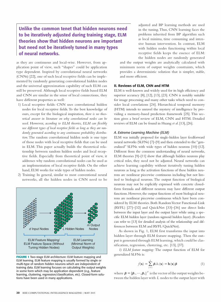
Fully connected hidden nodes, as shown in Fig. 2(a), have been extensively studied. Constructed from them, ELM achieves state-of-the-art performance for plenty of applications, such as remote sensing [51], time series analysis [52], text classi-fication [53], action recognition [20], etc.

However, these works focus only on random weights, while ignoring the attribute of random connections. For natural images and languages, the strong local correlations may make the full con-nections less appropriate. To overcome the problem, we propose to use hidden nodes which are locally connected with the input ones. According to ELM theories [9]–[11] the connections are ran-domly sampled based on certain probability distributions, which are denser around some input nodes while sparser farther away.

B. Local receptive Fields Based ELMA locally dense connection example of ELM-LRF is given in Fig. 2(b) in which the connections between input layer and hidden node i are randomly generated according to some continuous probability distribution, and some receptive field is generated by this random connections. The connections are dense around some input nodes and sparse farther away (yet do not completely disappear in this example).

Solid biological evidence also justifies the local receptive fields, which shows that each cell in the visual cortex is only sensitive to a corresponding sub-region of the retina (input layer) [54]–[56]. ELM-LRF learns the local structures and gen-erates more meaningful representations at the hidden layer when dealing with image processing and similar tasks.

C. Combinatorial NodeLocal receptive fields may have different forms in biological learning, and they may be generated in different ways using machine learning techniques. One of the methods is the combi-natorial node suggested in ELM theory [10]. ELM shows that a hidden node in ELM could be a combination of several hidden nodes or a subnetwork of nodes. For example, local receptive fields shown in Fig. 3 could be considered as a case where com-binatorial node i is formed by a subnetwork (as grouped by the circle). The output of this subnetwork is actually a summation (which need not be linear) of the output of three hidden nodes linking to corresponding local receptive fields of the input layer.

Thus, the feature generated at one location (one particu-lar hidden node) tends to be useful at different locations.

Hidden Node i

Hidden Node i

(a) Hidden Node in Full Connection

(b) Hidden Node in Local Connection

FiguRE 2 ELM hidden node in full and local connections: Random connections generated due to various continuous distributions.

Elm theories may shed a light on the research of different local receptive fields including true biological receptive fields of which the exact shapes and formula may be unknown to human beings.


Thus, the ELM-LRF network will be invariant to minor translations and rotations. Moreover, the connections between the input and combinatorial nodes may learn the local structures even better: denser connections around the input node because of the overlap of three receptive fields (see Fig. 3) while sparser farther away. Averaging and max-pooling methods are straightforward to formulate these combinatorial nodes. Additionally, learning-based method is also potential to construct them.

IV. the Implementation of local Receptive Fields

A. Specific Combinatorial Node of ELM-LrFAlthough different types of local receptive fields and combina-torial nodes can be used in ELM, for the convenience of imple-mentation, we use the simple step probability function as the

sampling distribution and the square/square-root pooling struc-ture to form the combinatorial node. The receptive field of each hidden node will be composed of input nodes within a prede-termined distance to the center. Furthermore, simply sharing the input weights to different hidden nodes directly leads to the convolution operation and can be easily implemented.

In this way, we build a specific case (Fig. 4) for the general ELM-LRF:1) Random convolutional node in the feature map in Fig. 4 is

a type of the locally connected hidden node in Fig. 3.2) Node in the pooling map in Fig. 4 is an example of the

combinatorial node shown in Fig. 3.

B. random input WeightsIn order to obtain thorough representations of the input, K different input weights will be adopted and K diverse feature maps are generated. And Fig. 5 depicts the implementation net-work we use with all K maps in this paper.

In Fig. 5, hidden layer is composed of random convolutional nodes. And the input weights of the same feature maps are shared while distinct among different maps. The input weights are randomly generated and then orthogonalized as follows:1) Generate the initial weight matrix A initt randomly1. With

the input size d d# and receptive field ,r r# the size of the feature map should be ( ) ( ) .d r d r1 1#- + - +

, , ,

A Ra R k K1

init

init

r K

kr

2

2

g

!

! =

#tt

(17)

2) Orthogonalize the initial weight matrix A initt using singular value decomposition (SVD) method. Columns of ,At akt ’s, are the orthonormal basis of A initt 2.

The orthogonalization allows the network to extract a more complete set of features than non-orthogonal ones. Hence, the generalization performance of the network is further improved. Orthogonal random weights have also been used in [5], [57] and produce great results.

The input weight to the k-th feature map is ,a Rkr r! #

which corresponds to a Rkr2!t column-wisely. The convolu-

tional node ( , )i j in the k-th feature map, ,c , ,i j k is calculated as:

( )

, , , ( )

xc x a

i j d r1 1

, , , , ,i j k i m j nn

r

m

r

m n k1 111

$

g

=

= - +

+ - + -

==

//

(18)

Several works have demonstrated that CNN with certain structure is also able to present surprisingly good performance with ELM feature mapping (through nonlinear mapping after random input weights [22], [58], [59]). However, the perfor-mance in these previous works are worse than fine-tuned ones. In this paper, the proposed ELM-LRF, where the input weights

1In this specific random convolutional node case, we find that the bias is not required in the hidden nodes. And we generate the random input weights from the standard Gaussian distribution.2In the case r 2 < K, orthogonalization cannot be performed on the column. Instead, the approximation method is used: 1) A

initt is transposed; 2) orthogonalized; 3) transposed back.

FiguRE 4 Although ELM-LRF supports wide type of local receptive fields as long as they are nonlinear piecewise continuous, a random convolutional node can be considered as a specific combinatorial node of ELM-LRF.

Local ReceptiveField

CombinatorialNode

Input Map Feature Map k

Random InputWeight ak

Pooling Map k

PoolingSize e

Combinatorial Node i

FiguRE 3 The combinatorial node of ELM [10]: a hidden node can be a subnetwork of several nodes which turn out to form local recep-tive fields and (linear or nonlinear) pooling.


to the feature maps are orthogo-nal random, can achieve even better performance than well-trained counterpart. Additionally the relationship between ELM-LRF and CNN will be dis-cussed later.

C. Square/Square-root pooling StructureThe square/square-root pooling structure is used to formulate the combinatorial node. Pooling size e is the distance between the center and the edge of the pooling area as shown in Fig. 5. And the pooling map is of the same size with the feature map ( ) ( ) .d r d r1 1#- + - + c , ,i j k and h , ,p q k respectively denote node ( , )i j in the k-th feature map and combinatorial node ( , )p q in the k-th pooling map.

, , , ( )

if ( , ) is out of bound:

h c

p q d ri j c

1 10

, , , ,( )( )

, ,

p q k i j kj q e

q e

i p e

p e

i j k

2

g

=

= - +

=

= -

+

= -

+

//

(19)

The square and summation operations respectively introduce rectification nonlinearity and translational invariance into the net-work, which have been discovered to be the essential factors for successful image processing and similar tasks [60]. Furthermore, the square/square-root pooling structure followed convolution opera-tion has been proved to be frequency selective and translational invariant [58]. Therefore, the implementation network we use in this paper will be especially suitable for image processing.

D. Closed-Form Solution Based output WeightsThe pooling layer is in full connection with the output layer as shown in Fig. 5. The output weights b are analytically cal-culated as in the unified ELM [12] using regularized least-squares method [61].

For one input sample ,x the value of combinatorial node h , ,p q k is obtained by calculating (18) and (19) cascadingly:

( )xc x a, , , , ,i j k i m j nn

r

m

r

m n k1 111

$= + - + -

==

//

h c, , , ,( )( )

p q k i j kj q e

q e

i p e

p e2=

= -

+

= -

+

//

, , , ( )

if ( , ) is out of bound:

p q d r

i j c

1 1

0, ,i j k

g= - +

=

(20)

Simply concatenating the values of all combinatorial nodes into a row vector and putting the rows of N input samples

together, we obtain the combinatorial layer matrix H :R ( )N K d r 1 2

! # $ - +

1) if ( )N K d r 1 2$# - +

H I HH TCT T 1

b = +-` j (21)

2) if ( )N K d r 1> 2$ - +

I H H H TCT T1

b = +-` j (22)

V. Discussions

A. Universal Approximation and Classification CapabilityELM-LRF with local randomly connected hidden nodes can be regarded as a specific type of ELM:1) Different density of network connections can be built

according to some type of continuous probability distribu-tion. According to ELM theories (e.g., Theorems 2.1 and 2.2), such networks still have universal approximation and classification capabilities.

2) Disconnected input nodes and hidden nodes can be consid-ered as connected by links with insignificant weights which can be neglected while dense connections are randomly generated with some type of continuous probability distri-bution. Overall speaking, the probability distribution which is used to generate such connections is still continuous, and thus, ELM with such local receptive fields still remains its universal approximation and classification capabilities.

3) Moreover, hidden nodes in ELM can be the combination of different computational nodes in linear or nonlinear manner, which naturally results in local receptive fields.

As those hidden nodes are usually nonliner piecewise con-tinuous as stated in Theorems 2.1 and 2.2, their combinatorial

FiguRE 5 The implementation network of ELM-LRF with K maps.

InputLayer

HiddenLayer

CombinatorialLayer

OutputLayer

LocalReceptive

Field

FeatureMap 1

FeatureMap K

PoolingSize e

1

i

m

PoolingMap K

FullConnection

OutputWeightsb

Random InputWeight a1

Random InputWeight aK

ELM Feature Mappingwith Random Convolutional Nodes

ELM Learning

Pooling Map 1


node ( , )p q in the k-th pooling map h , ,p q k can still generally be expressed as the basic form of ELM hidden node (2):

( , , ), , , , ( )a xh G b p q d r1 1, , , ,p q k p q p q g= = - + (23)

Apparently the function G provided by the square/squareroot pooling structure is nonlinear piecewise continuous. Therefore, the universal approximation and classification capabilities are preserved for ELM-LRF, enabling it to learn sophisticated forms of input data.

B. relationships with hTM and CNNThe implementation of ELM-LRF shares some resemblance with HTM [25] in the sense that through constructing the learning model layer-by-layer, they both mimic the brain to deal with increasingly complex forms of input. However, ELM-LRF is more efficient as the connections and input weights are both randomly generated while HTM might re-quire to carefully design the network and tune the parameters.

In addition, the proposed ELM-LRF is also closely related to CNN. They both handle the raw input directly and apply local connections to force the network to learn spatial corre-lations in natural images and languages. Subsequently, high-level features are implicitly learned or generated, on which the learning is subsequently performed. However, several dif-ferences exist between ELM-LRF and CNN:1) Local receptive fields: ELM-LRF provides more flexible and

wider type of local receptive fields, which could be sampled

randomly based on different types of probability distribu-tions. However, CNN only uses convolutional hidden nodes. Although this paper simply chooses random convolutional nodes as a specific local receptive field of ELM-LRF, it is worth investigating other suitable local receptive fields and learning methods to formulate the combinatorial nodes as the local receptive fields in biological learning (e.g. brains) may be unknown but their learning capabilities have been guaranteed by ELM theories.

2) Training: Hidden nodes in CNN need to be tuned and BP method is usually adopted. Thus, CNN faces the trivial issues associated with BP, such as local minima and slow conver-gence rate. In contrast, ELM-LRF randomly generates the input weights and analytically calculates the output weights. Only the calculation of output weights involves major com-putations, making ELM-LRF deterministic and efficient.

ELM feature mapping has also been used in some CNN net-work implementation (with random convolutional weights) [58]. However, the feature maps and pooling maps are collectively used as the input to a support vector machine (SVM) for learning [58]. Our proposed ELM-LRF simply uses a genuine ELM architecture with combinatorial nodes as hidden nodes in ELM feature mapping stage while keeping the rest ELM learning mechanism unchanged.

VI. ExperimentsThe proposed ELM-LRF has been compared with state-of-the-

art deep learning algorithms on NORB object recognition dataset [62], which is often used as a benchmark database by deep learning community. NORB dataset contains 24300 stereo images for training and 24300 ste-reo images for testing, each belonging to 5 generic categories with many variabilities such as 3D pose and lighting. Fig. 6 displays some examples from the dataset. Each sample has 2 images (left and right sides) with normalized object size and uniform background. We downsize them to 32 32# with-out any other preprocessing.

The experimental platform is MATLAB 2013a, Intel Xeon E5-2650, 2GHz CPU, 256GB RAM. In ELM-LRF, parameters that need to be tuned include: 1) size of receptive field { ,4 4# 6 6# }; 2) number of feature maps {24, 36, 48, 60}; 3) pooling size {1, 2, 3, 4}; 4) value of C {0.01, 0.1, 1, 10, 100}. We use a hold-out valida-tion set to choose the optimal parameters and list them in Table 1.

FiguRE 6 60 samples of NORB dataset.

Four-LeggedAnimals

Four-LeggedAnimals

HumanFigures

Airplanes Trucks CarsHumanFigures

Airplanes Trucks Cars

TaBLE 1 Optimal parameters.

DaTaSET# OF TRaiNiNg DaTa

# OF TESTiNg DaTa

iNPuT DiMENSiONS

RECEPTiVE FiELD

# OF FEaTuRE MaPS

POOLiNg SiZE C

NORB 24300 24300 32 # 32 # 2 4 # 4 48 3 0.01


A. Test ErrorThe test errors of other algorithms have been reported in liter-ature and summarized in Table 23. ELM-LRF produces better accuracy than other fine-tuned algorithms that requires much more computations. Compared with the conventional deep learning solutions, CNN and DBN, the proposed ELM-LRF reduces the test error rate from 6.5% to 2.74%. Our proposed ELM-LRF achieves the best accuracy compared to those results reported in literature with a significant gap.

B. Training TimeFor the training time, other algorithms are reproduced on our experimental platform to conduct a fair comparison. As shown in Table 3, ELM-LRF learns up to 200 times faster than other algorithms. And even compared with the random weights method [58], which is the current most efficient algorithm, ELM-LRF still achieves 4.48 times speedup and reaches much higher testing accuracy.

C. Feature MapsFig. 7 uses one data sample (airplane, the left image) for illustra-tion. And it also displays the corresponding 48 feature maps

3Although we tried to reproduce the results of other algorithms, we find that it is hard to reach similar accuracy as reported in literature due to tedious parameters tuning and time-consuming human intervention in conventional deep learning methods.

generated in the hidden layer. It can be observed that the out-lines of these feature maps are similar, as they all are generated from the same input image (an airplane). However, each map has its distinct highlighted part such that diverse representations of the original image are obtained. Collectively, these feature maps represent different abstractions of the original image, making the subsequent classification easy and accurate.

D. orthogonalization of random input WeightsIn our experiments, we have also investigated the contribu-tion of orthogonalization after the random generation of input weights. The values of the center convolutional nodes in the 48 feature maps are taken for example. The value dis-tributions generated by orthogonal and non-orthogonal ran-dom weights are shown in Fig. 8. One data sample is picked from each generic category. As observed from Fig. 8, the dis-tribution of orthogonal random weights spreads more broadly and evenly. It is similar for convolutional nodes occupying other positions in the feature maps. Therefore, orthogonaliza-tion will make the objects more easily to be linearly separated and classified.

In addition, even without orthogonalization, ELM-LRF can still achieve 4.01% test error, which is 38% decrease comparing to conventional deep learning methods, as shown in Table 2. Moreover, if considering the superb efficiency, ELM-LRF (no

TaBLE 3 training time comparison.

aLgORiTHMSTRaiNiNg TiME (S)

SPEEDuP TiMES1

ELM-LRF 394.16 217.47ELM-LRF (NO ORTHOGONALIZATION) 391.89 218.73RANDOM WEIGHTS2 (ELM FEATuRE MAppING + SVM CLASSIFIER)

1764.28 48.58

K-MEANS + SOFT ACTIVATION3 6920.47 12.39TILED CNN4 15104.55 5.67CNN5 53378.16 1.61DBN6 85717.14 11DBN IS uSED AS THE STANDARD TO CALCuLATE THE SpEEDup TIMES. 2 THE LATEST FASTEST CNN SOLuTION. THE TRAINING TIME REpORTED IN [58] IS 0.1H. REASONS FOR SuCH DIFFERENCE IN TRAINING TIME ARE: I) WE HAVE CON-SIDERED CONVOLuTION AND pOOLING OpERATIONS AS pART OF TRAINING, AND THE TRAINING TIME REpORTED INCLuDES THE TIME SpENT ON CONVOLuTION AND pOOLING, WHICH WERE NOT CONSIDERED IN [58]; II) ExpERIMENTS ARE RuN IN DIFFERENT ExpERIMENTAL pLATFORMS.

3uSE THE SAME pARAMETERS AS IN [60] WITH 4000 FEATuRES.4 uSE THE SAME ARCHITECTuRE AS ELM-LRF AND SET THE MAxIMuM NuMBER OF ITERATIONS IN THE pRETRAINING TO 20.

5 THE ARCHITECTuRE IS pROVIDED IN [62] AND WE uSE 50 EpOCHS.6 THE ARCHITECTuRE IS: 2048 (INpuT)-500-2000-500-5 (OuTpuT) AND 500 EpOCHS SINCE THE CONVERGENCE OF TRAINING ERROR IS SLOW WHEN DEALING WITH NORB DATASET.

FiguRE 7 One sample: the original image (left) and corresponding feature maps.

(a) The Original Image (Left One)

(b) The 48 Feature Maps

TaBLE 2 test error rates of different algorithms.

aLgORiTHMS TEST ERROR RaTESELM-LRF 2.74%ELM-LRF (NO ORTHOGONALIZATION) 4.01%RANDOM WEIGHTS [58] (ELM FEATuRE MAppING + SVM CLASSIFIER)

4.8%

K-MEANS + SOFT ACTIVATION [60] 2.8%TILED CNN [57] 3.9%CNN [62] 6.6%DBN [63] 6.5%


orthogonalization) is also an excellent solution for image pro-cessing and similar applications.

VII. ConclusionsThis paper studies the local receptive fields of ELM (ELM-LRF) which naturally results from the randomness of hidden neurons and combinatorial hidden nodes suggested in ELM theories. According to ELM theories, different types of local receptive fields can be used and there exists close relationship between local receptive fields and random hidden neurons. The local connections between input and hidden nodes may allow the network to consider local structures and combinatorial nodes further introduce translational invariance into the net-work. Input weights are randomly generated and then orthog-onalized in order to encourage a more complete set of features. The output weights are calculated analytically in ELM-LRF, providing a simple deterministic solution.

In the implementation, we construct a specific network for simplicity using the step function to sample the local connec-tions and the square/square-root pooling structure to formulate the combinatorial nodes. Surprisingly random convolutional nodes can be considered an efficient implementation of local receptive fields of ELM although many different types of local receptive fields are supported by ELM theories. Experiments conducted on the benchmark object recognition task, NORB dataset, show that the proposed ELM-LRF presents the best accuracy in the literature and accelerate the training speed up to 200 times compared to popular deep learning algorithms.

ELM theories show that different local receptive fields in ELM-LRF (and biological learning mechanisms) may be gen-erated due to different probability distribution used in generat-ing random hidden neurons. It may be worth investigating in the future: 1) the impact of different ELM local receptive fields; 2) the impact of different combinatorial hidden nodes of ELM;

3) stacked network of ELM-LRF modules performing unsu-pervised learning on higher-level abstractions.

Strictly speaking, from network architecture point of view, this paper simply uses one hidden layer of ELM although a combinatorial hidden layer is used. Stacked networks have been extensively investigated, such as stacked autoencoders (SAE), deep belief network (DBN) and convolutional DBN [63]–[66]. It deserves further exploration to construct the stacked net-work of ELM-LRF, by performing subsequent local connec-tions on the output of the previous combinatorial layer. The stacked network will capture and learn higher-level abstrac-tions. Thus, it should be able to deal with even more complex forms of input. In addition, unsupervised learning method, such as ELM Auto-Encoder (ELM-AE) [5], might be helpful for the stacked network to obtain more abstract representations without losing salient information.

AcknowledgmentThe authors would like to thank C. L. Philip Chen from Univer-sity of Macau, Macau for the constructive and fruitful discussions.

References[1] C. P. Chen and C.-Y. Zhang, “Data-intensive applications, challenges, techniques and technologies: A survey on big data,” Inform. Sci., vol. 275, pp. 314–347, Aug. 2014.[2] Z.-H. Zhou, N. Chawla, Y. Jin, and G. Williams, “Big data opportunities and chal-lenges: Discussions from data analytics perspectives,” IEEE Comput. Intell. Mag., vol. 9, pp. 62–74, Nov. 2014.[3] Y. Zhai, Y.-S. Ong, and I. Tsang, “The emerging ‘big dimensionality,’” IEEE Comput. Intell. Mag., vol. 9, pp. 14–26, Aug. 2014.[4] I. Arnaldo, K. Veeramachaneni, A. Song, and U. O’Reilly, “Bring your own learner: A cloud-based, data-parallel commons for machine learning,” IEEE Comput. Intell. Mag., vol. 10, pp. 20–32, Feb. 2015.[5] L. L. C. Kasun, H. Zhou, G.-B. Huang, and C. M. Vong, “Representational learning with extreme learning machine for big data,” IEEE Intell. Syst., vol. 28, no. 6, pp. 31–34, 2013.[6] D. E. Rumelhart, G. E. Hinton, and R. J. Williams, “Learning representations by back-propagation errors,” Nature, vol. 323, pp. 533–536, Oct. 1986.[7] G.-B. Huang, Q.-Y. Zhu, and C.-K. Siew, “Extreme learning machine: A new learn-ing scheme of feedforward neural networks,” in Proc. Int. Joint Conf. Neural Networks, July 2004, vol. 2, pp. 985–990.

FiguRE 8 The value distributions of the center convolutional nodes in the 48 feature maps with orthogonal and non-orthogonal random weights.

-0.2

0.2

0.1

0 0

-0.1

0 10 20 30Class 4

40 50-1

1

0.5

-0.5

0 10 20 30Class 5

40 50

Orthogonal WeightsNon-Orthogonal Weights

-0.4

0.4

0.2

0

-0.2

0 10 20 30Class 1

40 50-0.4

0.4

0.2

0

-0.2

0 10 20 30Class 2

40 50-0.3

0.2

0.1

0

-0.2

-0.1

0 10 20 30Class 3

40 50


[8] G.-B. Huang, Q.-Y. Zhu, and C.-K. Siew, “Extreme learning machine: Theory and applications,” Neurocomputing, vol. 70, pp. 489–501, Dec. 2006.[9] G.-B. Huang, L. Chen, and C.-K. Siew, “Universal approximation using incremental constructive feedforward networks with random hidden nodes,” IEEE Trans. Neural Net-works, vol. 17, no. 4, pp. 879–892, 2006.[10] G.-B. Huang and L. Chen, “Convex incremental extreme learning machine,” Neuro-computing, vol. 70, pp. 3056–3062, Oct. 2007.[11] G.-B. Huang and L. Chen, “Enhanced random search based incremental extreme learning machine,” Neurocomputing, vol. 71, pp. 3460–3468, Oct. 2008.[12] G.-B. Huang, H. Zhou, X. Ding, and R. Zhang, “Extreme learning machine for regression and multiclass classif ication,” IEEE Trans. Syst. Man, Cybern. B, vol. 42, no. 2, pp. 513–529, 2012.[13] G.-B. Huang, “An insight into extreme learning machines: Random neurons, ran-dom features and kernels,” Cognitive Comput., vol. 6, no. 3, pp. 376–390, 2014.[14] Z.-H. You, Y.-K. Lei, L. Zhu, J. Xia, and B. Wang, “Prediction of protein-protein interactions from amino acid sequences with ensemble extreme learning ma-chines and principal component analysis,” BMC Bioinform., vol. 14, suppl. 8, p. S10, 2013.[15] Y. Song, J. Crowcroft, and J. Zhang, “Automatic epileptic seizure detection in EEGs based on optimized sample entropy and extreme learning machine,” J. Neurosci. Methods, vol. 210, no. 2, pp. 132–146, 2012.[16] Y. Zhang and P. Zhang, “Optimization of nonlinear process based on sequential ex-treme learning machine,” Chem. Eng. Sci., vol. 66, no. 20, pp. 4702–4710, 2011.[17] Y. Yang, Y. Wang, and X. Yuan, “Bidirectional extreme learning machine for regres-sion problem and its learning effectiveness,” IEEE Trans. Neural Networks Learning Syst., vol. 23, no. 9, pp. 1498–1505, 2012.[18] Z. Yan and J. Wang, “Robust model predictive control of nonlinear systems with unmodeled dynamics and bounded uncertainties based on neural networks,” IEEE Trans. Neural Networks Learning Syst., vol. 25, no. 3, pp. 457–469, 2014.[19] A. Nizar, Z. Dong, and Y. Wang, “Power utility nontechnical loss analysis with ex-treme learning machine method,” IEEE Trans. Power Syst., vol. 23, no. 3, pp. 946–955, 2008.[20] R. Minhas, A. A. Mohammed, and Q. M. J. Wu, “Incremental learning in human action recognition based on snippets,” IEEE Trans. Circuits Syst. Video Technol., vol. 22, no. 11, pp. 1529–1541, 2012.[21] Y. Zhou, J. Peng, and C. L. P. Chen, “Extreme learning machine with composite kernels for hyperspectral image classif ication,” IEEE J. Select. Topics Appl. Earth Observ. Remote Sensing, 2014, to be published.[22] K. Jarrett, K. Kavukcuoglu, M. Ranzato, and Y. LeCun, “What is the best multi-stage architecture for object recognition?” in Proc. IEEE Int. Conf. Computer Vision, 2009, pp. 2146–2153.[23] Z. Bai, G.-B. Huang, D. Wang, H. Wang, and M. B. Westover, “Sparse extreme learning machine for classif ication,” IEEE Trans. Cybern., vol. 44, no. 10, pp. 1858–1870, 2014.[24] S. Lawrence, C. L. Giles, A. C. Tsoi, and A. D. Back, “Face recognition: A convolu-tional neural-network approach,” IEEE Trans. Neural Networks, vol. 8, no. 1, pp. 98–113, 1997.[25] J. Hawkins and S. Blakeslee, On Intelligence. New York: Macmillan, 2007.[26] G. Huang, G.-B. Huang, S. Song, and K. You, “Trends in extreme learning ma-chines: A review,” Neural Netw., vol. 61, no. 1, pp. 32–48, 2015.[27] Y.-H. Pao, G.-H. Park, and D. J. Sobajic, “Learning and generalization character-istics of the random vector functional-link net,” Neurocomputing, vol. 6, pp. 163–180, Apr. 1994.[28] C. P. Chen, “A rapid supervised learning neural network for function interpola-tion and approximation,” IEEE Trans. Neural Networks, vol. 7, no. 5, pp. 1220–1230, 1996.[29] C. Chen, S. R. LeClair, and Y.-H. Pao, “An incremental adaptive implementation of functional-link processing for function approximation, time-series prediction, and system identif ication,” Neurocomputing, vol. 18, no. 1, pp. 11–31, 1998.[30] C. P. Chen and J. Z. Wan, “A rapid learning and dynamic stepwise updating algo-rithm for f lat neural networks and the application to time-series prediction,” IEEE Trans. Syst. Man, Cybern. B, vol. 29, no. 1, pp. 62–72, 1999.[31] Y.-H. Pao, Adaptive Pattern Recognition and Neural Networks. Boston, MA: Addison-Wesley Longman Publishing Co., Inc., 1989.[32] B. Igelnik and Y.-H. Pao, “Stochastic choice of basis functions in adaptive function approximation and the functional-link net,” IEEE Trans. Neural Networks, vol. 6, no. 6, pp. 1320–1329, 1995.[33] H. White, “An additional hidden unit test for neglected nonlinearity in multilayer feedforward networks,” in Proc. Int. Conf. Neural Networks, 1989, pp. 451–455.[34] T.-H. Lee, H. White, and C. W. J. Granger, “Testing for neglected nonlinearity in time series models: A comparison of neural network methods and standard tests,” J. Econo-metrics, vol. 56, pp. 269–290, 1993.[35] M. B. Stinchcombe and H. White, “Consistent specif ication testing with nuisance parameters present only under the alternative,” Econometric Theory, vol. 14, no. 3, pp. 295–324, 1998.[36] H. White, “Approximate nonlinear forecasting methods,” in Handbook of Economics Forecasting, G. Elliott, C. W. J. Granger, and A. Timmermann, Eds. New York: Elsevier, 2006, pp. 460–512.[37] G. Huang, S. Song, J. N. Gupta, and C. Wu, “Semi-supervised and unsupervised extreme learning machines,” IEEE Trans. Cybern., vol. 44, no. 12, pp. 2405–2417, 2014.

[38] A. Rahimi and B. Recht, “Uniform approximation of functions with random bas-es,” in Proc. 46th Annu. Allerton Conf. Communication, Control, Computing, Sept. 2008, pp. 555–561.[39] G.-B. Huang, Q.-Y. Zhu, K. Z. Mao, C.-K. Siew, P. Saratchandran, and N. Sunda-rarajan, “Can threshold networks be trained directly?” IEEE Trans. Circuits Syst. II, vol. 53, no. 3, pp. 187–191, 2006.[40] W. F. Schmidt, M. A. Kraaijveld, and R. P. Duin, “Feedforward neural networks with random weights,” in Proc. 11th IAPR Int. Conf. Pattern Recognition Methodology Sys-tems, 1992, pp. 1–4.[41] B. Widrow, A. Greenblatt, Y. Kim, and D. Park, “The no-prop algorithm: A new learning algorithm for multilayer neural networks,” Neural Netw., vol. 37, pp. 182–188, Jan. 2013.[42] G.-B. Huang, X. Ding, and H. Zhou, “Optimization method based extreme learning machine for classif ication,” Neurocomputing, vol. 74, pp. 155–163, Dec. 2010.[43] C. R. Rao and S. K. Mitra, Generalized Inverse of Matrices and Its Applications. vol. 7, New York: Wiley, 1971.[44] B. Frénay and M. Verleysen, “Using SVMs with randomised feature spaces: An ex-treme learning approach,” in Proc. 18th European Symp. Artificial Neural Networks, Apr. 28–30, 2010, pp. 315–320.[45] C. Cortes and V. Vapnik, “Support vector networks,” Mach. Learn., vol. 20, no. 3, pp. 273–297, 1995.[46] T. Poggio, S. Mukherjee, R. Rifkin, A. Rakhlin, and A. Verri, “b,” A.I. Memo No. 2001-011, CBCL Memo 198, Artif icial Intelligence Laboratory, Massachusetts Institute of Technology, Cambridge, MA, 2001.[47] I. Steinwart, D. Hush, and C. Scovel, “Training SVMs without offset,” J. Machine Learning Res., vol. 12, pp. 141–202, Feb. 2011.[48] P. L. Bartlett, “The sample complexity of pattern classif ication with neural networks: The size of the weights is more important than the size of the network,” IEEE Trans. Inform. Theory, vol. 44, no. 2, pp. 525–536, 1998.[49] D. H. Hubel and T. N. Wiesel, “Receptive f ields and functional architecture of mon-key striate cortex,” J. Physiol., vol. 195, no. 1, pp. 215–243, 1968.[50] D. Scherer, A. Müller, and S. Behnke, “Evaluation of pooling operations in convo-lutional architectures for object recognition,” in Proc. Int. Conf. Artificial Neural Networks, 2010, pp. 92–101.[51] M. Pal, A. E. Maxwell, and T. A. Warner, “Kernel-based extreme learning ma-chine for remote-sensing image classif ication,” Remote Sensing Lett., vol. 4, no. 9, pp. 853–862, 2013.[52] J. Butcher, D. Verstraeten, B. Schrauwen, C. Day, and P. Haycock, “Reservoir com-puting and extreme learning machines for non-linear time-series data analysis,” Neural Netw., vol. 38, pp. 76–89, Feb. 2013.[53] W. Zheng, Y. Qian, and H. Lu, “Text categorization based on regulariza-tion extreme learning machine,” Neural Comput. Applicat., vol. 22, nos. 3–4, pp. 447–456, 2013.[54] P. Kara and R. C. Reid, “Efficacy of retinal spikes in driving cortical responses,” J. Neurosci., vol. 23, no. 24, pp. 8547–8557, 2003.[55] D. L. Sosulski, M. L. Bloom, T. Cutforth, R. Axel, and S. R. Datta, “Distinct rep-resentations of olfactory information in different cortical centres,” Nature, vol. 472, no. 7342, pp. 213–216, 2011.[56] O. Barak, M. Rigotti, and S. Fusi, “The sparseness of mixed selectivity neurons controls the generalization-discrimination trade-off,” J. Neurosci., vol. 33, no. 9, pp. 3844–3856, 2013.[57] Q. V. Le, J. Ngiam, Z. Chen, D. Chia, P. W. Koh, and A. Y. Ng, “Tiled convolu-tional neural networks,” in Proc. Advances Neural Information Processing Systems, 2010, pp. 1279–1287.[58] A. Saxe, P. W. Koh, Z. Chen, M. Bhand, B. Suresh, and A. Y. Ng, “On random weights and unsupervised feature learning,” in Proc. Int. Conf. Machine Learning, 2011, pp. 1089–1096.[59] D. Cox and N. Pinto, “Beyond simple features: A large-scale feature search approach to unconstrained face recognition,” in Proc. IEEE Int. Conf. Automatic Face Gesture Recogni-tion Workshops, 2011, pp. 8–15.[60] A. Coates, A. Y. Ng, and H. Lee, “An analysis of single-layer networks in unsu-pervised feature learning,” in Proc. Int. Conf. Artificial Intelligence Statistics, 2011, pp. 215–223.[61] D. W. Marquaridt, “Generalized inverses, ridge regression, biased linear estimation, and nonlinear estimation,” Technometrics, vol. 12, no. 3, pp. 591–612, 1970.[62] Y. LeCun, F. J. Huang, and L. Bottou, “Learning methods for generic object rec-ognition with invariance to pose and lighting,” in Proc. Int. Conf. Computer Vision Pattern Recognition, July 2004, vol. 2, pp. II-97–104.[63] V. Nair and G. E. Hinton, “3D object recognition with deep belief nets,” in Proc. Advances Neural Information Processing Systems, 2009, pp. 1339–1347.[64] Y. Bengio, “Learning deep architectures for AI,” Foundations Trends R Machine Learn-ing, vol. 2, no. 1, pp. 1–127, 2009.[65] M. A. Ranzato, C. Poultney, S. Chopra, and Y. LeCun, “Efficient learning of sparse representations with an energy-based model,” in Proc. Advances Neural Information Process-ing Systems, 2006, pp. 1137–1144.[66] H. Lee, R. Grosse, R. Ranganath, and A. Y. Ng, “Convolutional deep belief net-works for scalable unsupervised learning of hierarchical representations,” in Proc. Int. Conf. Machine Learning, 2009, pp. 609–616.

Local Receptive Fields Based Extreme Learning Machine · Abstract—Extreme learning machine ......

Documents

Transcript of Local Receptive Fields Based Extreme Learning Machine · Abstract—Extreme learning machine ......