1

Local Cooperativity Mechanism in the DNA

Melting Transition

Vassili Ivanov1, Dmitri Piontkovski2, and Giovanni Zocchi1

1 Department of Physics and Astronomy, University of California Los Angeles,

Los Angeles, CA 90095-1547, USA

2 Central Institute of Economics and Mathematics, Nakhimovsky prosp. 47,

Moscow 117418, Russia

We propose a new statistical mechanics model for the melting transition of DNA. Base pairing

and stacking are treated as separate degrees of freedom, and the interplay between pairing and

stacking is described by a set of local rules which mimic the geometrical constraints in the real

molecule. This microscopic mechanism intrinsically accounts for the cooperativity related to the

free energy penalty of bubble nucleation. The model describes both the unpairing and unstacking

parts of the spectroscopically determined experimental melting curves. Furthermore, the model

explains the observed temperature dependence of the effective thermodynamic parameters used in

models of the nearest neighbor (NN) type. We compute the partition function for the model

through the transfer matrix formalism, which we also generalize to include non local chain

entropy terms. This part introduces a new parametrization of the Yeramian-like transfer matrix

approach to the Poland-Scheraga description of DNA melting. The model is exactly solvable in

the homogeneous thermodynamic limit, and we calculate all observables without use of the grand

partition function. As is well known, models of this class have a first order or continuous phase

transition at the temperature of complete strand separation depending on the value of the

exponent of the bubble entropy.

2

I. INTRODUCTION

Conformational transitions are a major area of research in the physics of biological

polymers, and in this area DNA melting represents one model problem, because of its

relative simplicity compared for instance to protein folding. The stable conformation of

double stranded (ds) DNA at room temperature is the double helix. The two strands are

held together by hydrogen bonds between Watson-Crick complementary base pairs (bp):

A-T, stabilized by 2 hydrogen bonds ( 37 310 ~ 1.5 oBG k T∆ ), and G-C, with 3 hydrogen

bonds ( 37 310 ~ 3 oBG k T∆ ) [1]. The next conformationally important attractive interaction

is between adjacent bases on the same strand. This interaction favors keeping successive

bases of the same strand stacked like a deck of cards, and is refereed to as stacking. The

main destabilizing interaction is the repulsive electrostatic force between the negatively

charged phosphate groups on either strand; this interaction can be modulated through the

ionic strength of the solvent. As the temperature is raised, two processes alter the double

helical conformation: base pairs may break apart, giving rise to bubbles of single stranded

(ss) DNA, and bases may unstack along the single strands [2]. At the critical temperature

where the two strands completely separate, there can still be significant stacking (i.e.

secondary structure) in the single strands; this melts away as the temperature is raised

further, the single strands finally resembling random coils at sufficiently high temperature.

Simplified statistical mechanics models of the transition (i.e. models with a reduced

number of degrees of freedom compared to the real molecule) have a multiplicity of

purposes, from quickly predicting melting temperature for applications such as PCR

primer design, to studying the nature of the phase transition (whether continuous or

discontinuous, for instance) and how it depends on sequence disorder, applied fields, etc.

Indeed, to extract the thermodynamic parameters related to DNA melting from the

experimental measurements requires a statistical mechanics model specifying the states in

configuration space to which the free energies to be measured refer. For practical

purposes, the nearest neighbor (NN) thermodynamic model [3] gives adequate

predictions. In this model, the free energies for all possible dimer combinations (i.e.

double stranded (ds) sequences of length 2) are assigned, and the total free energy is the

sum of the dimer free energies for the specific sequence. Since there are 10 different

dimers, this model has 10 parameter sets. Pairing and stacking interactions are lumped

together into effective free energies of the dimer. Most theoretical investigations of the

3

nature of the melting transition have on the other hand been carried out using models of

the Poland-Scheraga (PS) kind or the Peyrard-Bishop (PB) kind. In the PS type models,

the partition function for the molecule is written as a sum over bubble states [4–7]. A

considerable effort has been devoted to the non trivial question of the correct statistical

weights for the bubbles and the order of the phase transition in the thermodynamic limit

[8,9]; by contrast, here we focus on the question of which degrees of freedom are crucial

for a statistical mechanics description of oligomer melting curves. The PB approach is

based on an effective Hamiltonian for the molecule which contains potential energy terms

for the relative motion of opposite bases on the two strands as well as adjacent bases on

the same strand [10]. This is closest to our own approach described below, in that here a

local mechanism arising from the interplay of two different degrees of freedom is

responsible for the cooperative behavior of (or long range interactions along) the bubbles.

Modern developments of Peyrard-Bishop like Hamiltonian models were applied to

describe DNA unzipping under an external force [11–14].

In a previous paper [15] we underlined the notion that melting profiles of DNA

oligomers show the contribution of two different processes: unpairing of the

complementary bases on opposite strands, leading to local strand separation, and

unstacking of adjacent bases on the same strand, leading to loss of the residual secondary

structure of the single strands, i.e. to a random coil conformation of the ss. Accordingly,

if a model is to describe the melting profiles in the whole experimental temperature range,

including at temperatures beyond strand separation, but where residual stacking may still

be present in the ss, then pairing and stacking must be considered as separate degrees of

freedom in the model. In [15] we pursued this approach through a model combining a

description of stacking in terms of an Ising model and pairing in terms of a zipper model.

We showed by comparison with the experiments that the Ising model gives an adequate

description of stacking. However, the zipper model description of pairing [15], initially

adopted for simplicity, is unsatisfactory in that it considers only states where the

molecule unzips from the ends. Here we introduce an improved description, where

pairing and stacking are both Ising variables, there are only nearest neighbor interactions,

but there are constraints on the possible states of the fundamental dimer (two adjacent bp),

which represent the geometrical constraints in the real molecule. We detail the states of

the dimer below, but to give an example, one open bp followed by one closed bp means

necessarily at least one unstacking, translating into one out of all possible dimer states

4

being forbidden. Thus while in the zipper model the cooperativity of base pairing (i.e. the

tendency for base pairs to open in contiguous segments, or in other words the existence of

a nucleation penalty for the bubble) is put in “by hand”, here it results from a local

mechanism (the interplay between pairing and stacking). This idea is also present in the

PB models, and indeed our approach is closest to the PB and NN models, but differing in

the implementation of the underlying physics.

Stacking interactions in ss DNA were described years ago [16–18], but only 3 out of 16

stacking parameters have been measured precisely [2]. The major difficulty in the

measurements is to separate the contributions of pairing and stacking interactions. As a

result, the stacking interaction has not been incorporated into the DNA melting models as

a separate degree of freedom. In practice, stacking was included in the NN model [3] as a

correction to the pairing interaction parameter set. In the model below, we introduce

stacking as a separate interaction with its own set of thermodynamic parameters (stacking

enthalpy and entropy [3]). The thermodynamic parameters of the NN model can be

calculated from these separate paring and stacking parameters, and appear then to be

temperature dependent. We use the transfer matrix formalism to compute the partition

function for our model, and compare to the experimental melting curves. In Sec. V-VII

we extend this formalism to take into account the non local part of the loop entropies.

II. STATES OF THE NN DIMER

Let us consider the NN model dimer * *1 1i i i iB B B B+ + , 1, , 1i N= −K . The dimer has four

DNA bases arranged into two anti-parallel strands 1i iB B + and * *1i iB B+ (listed from 5’ to 3’

end). The pairing interaction is between complementary bases iB , *iB ; the stacking

interaction between adjacent bases iB , 1iB + and *1iB + , *

iB (considering stacking order

from 5’ to 3’ end). The free energies of the i -th stackings between the bases iB and 1iB +

of the B -strand and bases *1iB + and *

iB of the complimentary *B -strand are StiG and *St

iG

respectively, while PiG is the free energy of the i -th pairing between the bases iB and

*iB . The free energy parameters result from the corresponding entropies and enthalpies,

i i iG E TS= − . To simplify the notation we will use the statistical weights:

( )expP Pi iU Gβ= − , ( )expSt St

i iU Gβ= − , and ( )* *expSt Sti iU Gβ= − , where 1 Tβ = . The

5

model has a unique ground state - unmelted double helix with all bases paired and

stacked - and many different exited states, even after complete strand dissociation. All

thermodynamic parameters, i.e. pairing and stacking enthalpies, entropies, and free

energies, are referred to the ground state. Therefore, unlike in most of the literature, we

are dealing with positive energies and entropies of the excited states calculated with

respect to the ground state. In a dimer base pairing is shared with the complementary

bases (the stackings are not shared); therefore all pairings in the dimers will be counted

with coefficient 12 . We suggest that if both pairing interactions in the dimer are “closed”,

then the stacking interactions are necessarily also closed, while if both pairings are

“open”, then the stackings may be closed or open, the opening of the stackings resulting

in a free energy gain StiG or *St

iG . Thus in this description the free energy gain for

complete unpairing of the NN dimer is:

( ) ( ) ( )( )*1 2 ln 1 exp ln 1 expNN P P St St

i i i i iG G G T G Gβ β+ = + − + − + + − . (1)

where the argument of the logarithm is the partition function expressing the fact that the

unpaired dimer can be either stacked or unstacked. The enthalpy and entropy gain upon

melting of the NN dimer can be easily calculated from Eq. (1), and it is evident that these

effective thermodynamic parameters (which are the ones used in the NN model [3]) are

now temperature dependent. We come back to this point later.

Each nearest neighbor dimer has 2 stacking degrees of freedom and 2 pairing degrees

of freedom, which can each be open or closed, for a total of 24 = 16 possible states. We

introduce a local mechanism which gives rise to the cooperative behavior of the bubble,

by implementing two local geometrical constraints. The first is that unstacking of two

adjacent bases is only possible after unpairing of at least one of the bases. The second

constraint requires at least one stacking of the dimer open if one pairing is open and one

pairing closed. As a result, only 11 out of 16 states are admissible, Fig. 1. The

geometrical origin of the constraints is that pairing interactions can prevent unstacking,

and unpairing of exactly one out of two adjacent pairings requires spatial separation of

the unpaired bases, which is impossible without al least one unstacking. Thus for instance

Eq. (1) is applicable only for completely unpaired dimers, and not for partially melted

6

dimers. These constraints require mandatory unstacking at the beginning of the melting

fork, and therefore imply a penalty for opening a bubble.

FIG. 1. Each NN dimer has two pairings (vertical

lines) and two stackings (horizontal lines). The

broken bonds are crossed. The horizontal lines

represent the strands. There are sixteen states of the

dimer; admissible states of the NN model dimer are

the states from 1 to 11; the states from 12 to 16 are

prohibited by the geometric constraints.

III. TRANSFER MATRIX FORMALISM

It is convenient to write the partition function in the transfer matrix formalism; the

mathematics is the same as for instance in the corresponding treatment of the 1-D Ising

model of ferromagnetism [19] or the helix-coil transition in biopolymers [20,21]. Two

adjacent NN dimers share one pairing interaction. Therefore, the transfer matrix

technique for the model propagates the state of the pairing interactions only. The state of

the i -th pairing is described by the two component covector (string) ( ),0 ,1,i i iX x x= ,

1 i N≤ ≤ . The first covector 1X describes the boundary condition on the 5’ end of the

molecule. The covector component ,0ix describes the partition function of the i -mer with

the last pairing closed; ,1ix describes the case of the last pairing open. The 2 2× transfer

matrix iA transforms covector iX into covector 1i i iX X A+ = (there is no summation over

i ). The transfer matrix iA corresponds to the i -th NN dimer and contains the i -th

stacking, the i -th stacking of the complementary strand, and the i -th and 1i + pairings.

To calculate the partition function of the entire molecule we need a boundary condition

on the 3’ end which can be characterized by the two dimensional vector (column) NY . In

the following we will use free boundary conditions on the DNA molecule ends unless

otherwise specified, i.e. all possible states of the first and the last base pairs are

admissible. The vector ( ),0 ,1,T

i i iY y y= corresponds to the i -th pairing (from the 5’ end)

and can be calculated recursively from the 3’ end by: 1i i iY AY += . The partition function of

7

the whole DNA is the product of the 5’ end boundary condition vector 1X , ( )1N −

transfer matrixes corresponding to the NN dimers, and 3’ end boundary condition vector

NY :

1

11

N

N i Ni

Z X A Y−

=

= ∏ . (2)

The partition function can be also written as N i iZ X Y= , there is no summation, and any

i from 1 to N can be chosen. In the transfer matrix iA :

,00 ,01

,10 ,11

i ii

i i

a aA

a a

=

. (3)

the value 0 of the index of the matrix elements corresponds to closed pairing, and 1

corresponds to open pairing, i.e. the matrix element ,00 1ia = describes the ground state of

the dimer with all pairings closed; ,01ia describes the states with the first paring closed

and the second pairing open; ,10ia describes the states with the first pairing open and the

second closed; and ,11ia describes the states with both pairings open.

To write the explicit form of the matrix elements (3), note that ,00 1ia = corresponds to

diagram 1 in Fig. 1; ,01ia corresponds to diagrams 2, 3, 4; ,10ia corresponds to diagrams 6,

7, 8; and ,11ia is the statistical weight corresponding to the free energy Eq. (1), and

corresponds to diagrams 5, 10, 9, 11. The result for the transfer matrix is:

( )( ) ( )

* *1

* * * *1

1

1

P St St St Sti i i i i

iP St St St St P P St St St Sti i i i i i i i i i i

U U U U UA

U U U U U U U U U U U

+

+

+ + = + + + + +

(4)

The contributions of the pairing free energies are counted with coefficients 12 , or the

square root of the statistical weights. The sums correspond to summing the different

8

diagrams of Fig. 1 in the partition function; the products correspond to adding the free

energies of pairing and stacking.

The first and the last dimers do not have adjacent dimers on their 5’ or 3’ ends

respectively. The (co)vectors 1X and NY specifying the boundary conditions are

multiplied by the first and the last transfer matrix in the partition function (2). Covector

1X describes the first pairing interaction shared with the first dimer already described by

the transfer matrix 1A , and vector NY describes the last pairing shared with the last dimer

already described by the transfer matrix 1NA − . We include 12 of the pairing interaction

or the square root of the corresponding statistical weight into the 5’ boundary covector

1X and the 3’ vector NY :

( )1 11, PX U= , ( )1,T

PN NY U= . (5)

To include in the model the entropy gain DS due to complete strand dissociation, we

calculate the correction to the state with all pairings open:

( ) ( ) ( )1

*, 1 1

1

exp 1 1 1N

P P P P St StN D D N i i i i

i

Z S U U U U U U−

+=

= − + + ∏ . (6)

The final partition function is the sum of the partition function (2) and the correction (6):

,total N N DZ Z Z= + . (7)

To calculate any local observables, for example the probabilities of unstacking or

unpairing of some specific bond, we first calculate all X and Y vectors in advance. In

the form of the partition function:

,0 ,0 ,1 ,1N i i i i i iZ X Y x y x y= = + (8)

9

(valid for any i ), the first term is the partition function for the system with the i -th bp

closed, the second term is the partition function for the i -th bp open. Thus the probability

that the i -th bp is unpaired is:

( ) ,1 ,1unpair i i NP i x y Z= . (9)

Similarly, to calculate the probability that the i -th stacking of the primary strand is

unstacked, we take the product 1i i iX A Y , where the matrix 1

iA is derived from the matrix

iA in (5) by keeping only the Fig. 1 diagrams corresponding to this unstacking, in this

case diagrams 2, 4, 6, 8, 10, 11. Thus:

( )( ) ( )

*11

* *1

0 P St St Sti i i i

iP St St St P P St St Sti i i i i i i i i

U U U UA

U U U U U U U U U

+

+

+ = + +

(10)

and the required probability is :

( ) 11unstack i i i NP i X A Y Z+= . (11)

The average number of open bp is the sum ( )1

Nunpairi

P i=∑ , and similarly for unstacking.

In summary, the difference between the 2 2× model (described by Eqs. (2) and (3))

and the existing standard form of the NN model [3] is that the partially melted dimers are

considered specially. This internal structure of the dimers gives rise to a temperature

dependence of the effective NN model parameters, expressed in Eq. (1). We show below

that the 2 2× model is an improvement with respect to the NN model in describing

oligomer melting curves. There is however still at least one important piece of physics

missing from the model, namely a better estimate of the entropy of the bubbles (loops). In

the present model, as in the NN model, the number of states increases exponentially with

the length of the bubble, i.e. the entropy is linear in the bubble length. But in the real

system the bubble is a loop, which results in a logarithmic correction to the entropy. The

exact form of this correction (including excluded volume effects) has been addressed in

10

the PS type models [5, 6]. It is possible to include these effects in a generalization of the

present formalism which we present in Sec. V.

IV. RESULTS FOR THE 2x2 MODEL

A. Melting curves of oligomers

We compare the model to two oligomer sequences. The first oligomer sequence L13_2

used in the measurement is CG rich and forms no hairpins (CGA CGG CGG CGC G).

The second sequence L60 is partially selfcomplementary and has an AT rich tract in the

middle (CCG CCA GCG GCG TTA TTA CAT TTA ATT CTT AAG TAT TAT AAG

TAA TAT GGC CGC TGC GCC). L60 can form a hairpin, but the contribution of

hairpin states above the dissociation temperature is negligible [15].

For the experiments, synthetic oligomers were annealed in phosphate buffer saline

(PBS) at an ionic strength of 50 mM, pH = 7.4 and the UV absorption curve f was

measured at 260 nm, in a 1 cm optical path cuvette (see Fig. 2 (A1) and (B1)).

To compare the model with the experimental data, the UV absorption is assumed to be a

linear function of pairing and stacking:

( ) ( )( ) CsunstackingNunpairingsNf γδα +×−+×= )1(2 (12)

where C is the concentration of the ds oligomer, measured in mmol, α and δ are the

molar extinction coefficients for unpairing and unstacking, measured in mmol-1cm-1 (the

optical path being 1 cm). The UV curves were normalized so that 1=f corresponds to

strand dissociation. To measure the fraction of dissociated molecules p for L60 we use a

quenching technique which we have described before [22,23]. Briefly, to determine the

dissociation curve p (see Fig. 2 (A2)), the sample is heated at temperature iT , then

quenched to ~ 0o C. Because the sequence L60 is partially self-complementary, molecules

which were dissociated at temperature Ti form hairpins after the quench. The relative

number of hairpins (representing the fraction of dissociated molecules p at

temperature iT ) is determined by gel electrophoresis.

In Fig. 2 we display the melting curves from the experiments (symbols) and the model

(continuous lines). In Fig. 2 (A2) and (B2) we show the fraction of dissociated molecules

calculated from the model using the same parameter values as for the fit of the UV

11

absorption curves. The sequence L13-2 is not self-complementary, so in Fig. 2 (B2) we

show only the predicted dissociation curve.

For simplicity, in the fits the model was used with just one value for all stacking

thermodynamic parameters, namely, stacking enthalpy and entropy of 4500 K and 12

respectively. Also, for L13-2 (which is nearly homogeneous) we used just one set of

pairing enthalpy and entropy. Here and in the following we measure energies in degrees

Kelvin and entropies in units of Bk . The high value of the dissociation entropy for L60

reflects a deficiency of the model: if we introduce a logarithmic bubble entropy in the

form of Ref. [8], L60 can be fitted with the same dissociation entropy as for L13-2, while

the other parameters of the fit change only about 5%. We cure this anomaly in Sect. V.

TABLE I. Values of the thermodynamic parameters which produce good fits to the

experimental melting curves for L60 and L13-2, using the 2 2× model. Energies are

measured in Kelvins and entropies in units of Bk .

Oligomer DS PCGE P

CGS PATE P

ATS

L60 34 5040 14 2800 7.4

L13-2 9 5120 13.92 N/A N/A

B. Temperature dependence of the NN model parameters

Fig. 3 shows the specific heat calculated from the partition function (2) for the oligomer

L13-2. There is a gap in the specific heat on the two sides of the transition, which in this

model is due to the residual stacking bonds breaking in the single stranded DNA (after

strand separation). According to Fig. 3 the thermal capacity gain per dimer is about 78 at

a temperature of 90oC, which is roughly consistent with the literature values reviewed in

[24].

The thermodynamic parameters of the NN model can be calculated from the free

energy of the completely unpaired dimer, Eq. (1). The enthalpy calculated from Eq. (1) is

( ) * *1( ) 2 ( ) ( )NN P P St St St St

i i i i i i iE T E E P T E P T E+= + + + , (13)

and the entropy is:

12

( ) ( )( ) ( )( )

* *1

*

( ) 2 ( ) ( )

ln 1 exp 1 exp .

NN P P St St St Sti i i i i i i

St Sti i

S T S S P T E P T E

G G

β

β β

+= + + +

+ + − + − (14)

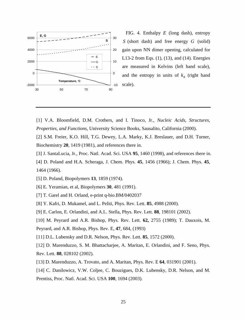
We plot these quantities in Fig. 4 for the oligomer L13-2 using the thermodynamic

parameters from the UV spectrum fit of Fig. 2 (B1) and (B2).

V. REFORMULATION OF THE MODEL TO INCLUDE THE POLAND –

SHERAGA BUBBLE ENTROPIES

In the PS model the states of the DNA are classified in terms of non-interacting bubbles.

The partition function counts all possible bubble states of the polymer and takes into

account cooperative effects within the bubbles. Namely, the bubbles are characterized by

the energy penalty of the broken bonds and the favorable entropy proportional to the

bubble size, as well as an energy penalty for the creation of the melting forks. If the

bubble is bounded by two ds segments, there is an extra entropy cost for terminating the

random walk of the DNA single strands at the end of the bubble (i.e. making a closed

loop). The energy penalty for the melting forks can, in our formalism, be absorbed into

the statistical weights describing opening ( 01a ) and closure ( 10a ) of the bubble, in a

sequence specific manner. The bubble entropy proportional to bubble size reflects the

entropy gain upon breaking of the pairing interaction; we absorb it into the statistical

weights describing open dimers ( 11a ). Then we are left with a bubble entropy of the form:

( ) lnBBS n C n= − . The constant BC depends on the dimension of the random walk; its

estimates can be found in an extensive literature [5, 6, 15, 17]. According to [3, 15, 17]

the order of the phase transition at the strand separation temperature in the

thermodynamic limit depends on the value of the constant BC . If 1BC ≤ , the average size

of the bubble is finite at any temperature and there is no phase transition. If 1 2BC< ≤ ,

the average size of size the bubble goes to infinity at the phase transition temperature and

the phase transition is continuous. If 2BC > , the average bubble size right before the

phase transition is finite and the phase transition is of the first order.

The usual approach to the PS model is to consider the “bubble” as a particle and to

calculate the grand partition function in the thermodynamic limit in terms of bubbles. The

13

use of the grand partition function requires a variable number of DNA bases and the

fugacity, which is not very transparent and non-constructive, i.e. the grand partition

function cannot be used for the calculation of the partition function of an inhomogeneous

DNA molecule of finite size, and is inefficient for calculating local quantities such as the

probability of opening a bubble of a given size in a given place.

The local states of the NN model dimer described by the transfer matrix (3) and

corresponding (co)vectors do not contain any information about the distance between

bases once they have separated, or the bubble size. The long range bubble entropy

penalty cannot be described by the 2 2× matrices. Therefore, we extend the algorithm

from the two-dimensional covectors iX (and corresponding vectors iY ) of the 2 2×

model to multidimensional covectors. While the covector component ,0ix still describes

the partition function of the i -mer with the last pairing closed, the covector component

,i nx ( 1n ≥ ) is the partition function of the i -th mer with exactly n open base pairs at the

3’ end of the subsequence. For example, ,1ix corresponds to the i th base pair open, with

the 1i − base pair closed. For the N -mer the maximal size of the bubble is N (the strand

dissociated state) and the maximal size of covector iX is 1N + .

We use the matrix elements of the transfer matrix iA introduced before to describe the

local states of the NN dimer and parametrize the extended ( ) ( )1 1N N+ × + transfer

matrix iD . The dimer with all base pairings closed is described by the matrix element

,00 ,00 1i id a= = . The dimer with the first base pair open and the second closed is

characterized by the matrix element ,01 ,01i id a= . The fully open dimers are described by

the matrix elements , 1 ,11i n n id a+ = , where the index n indicates how many bases are open

in the 5’ direction from the dimer. All bubble penalty effects (as well as the hairpin

formation effects) are taken into account at the site of the bubble closure and incorporated

into the corresponding matrix element ( ), 0 ,10B

i n i id U n a= , where ( ) ( )( )expB Bi iU n S n=

(for i n> ) are the statistical weights corresponding to the entropy penalty for closing the

bubble, and ( ) 1BiU i = since n i= corresponds to the melting fork at the 5’ end. All other

elements of the transfer matrix iD are equal to zero. Explicitly, for the system of size N

the covector iX has the form: ,0 ,1 ,( , , , )i i i i NX x x x= K , where ,0ix is the partition sum for

14

the system of size i with the last bp closed, while ,i nx (1 n i≤ ≤ ) is the partition sum for

the system of size i with the last n bp open. , 0i nx = for n i> , because the bubble

cannot be larger than the size of the sequence. The recursion relations in this notation are:

1,0 00 ,0 ,10 ,0

( ) Bi i i i i n

n

x a x a U n x+≠

= + ∑ , (15)

1, ,11 , 1 i n i i nx a x+ −= , 1n ≥ . (16)

The transfer matrix of the model written in table form is thus:

( )( )( )

01

10 11

10 11

10

1 0 01 0 02 0 03 0 0 0

B

B

B

aU a a

D U a aU a

=

LLLL

M M M M O

, (17)

where the index i is skipped for simplicity. The partition function of the oligomer can be

calculated using Eq. (2) with the transfer matrix (17) and the free boundary conditions

specified by the 5’ covector and 3’ vector:

( )1 11, ,0, ,0PX U= K , ( )( )1, , , ,expT

P P PN N N D NY U U S U= K . (18)

The square roots of the statistical weights in Eq. (18) count ½ of the pairing free energy

not included into the first and the last NN dimers, which corresponds to the NN model

[20] boundary corrections discussed in Sec. III. The last vector element ,N Ny corresponds

to the bubble of size equal to the oligomer length, i.e. the state with all pairings open and

separated strands. Therefore, the entropy gain upon strand dissociation DS is included in

the ,N Ny vector component providing the partition function of the dissociated state. If we

are not taking into consideration DS and the boundary condition effects, we can chose

15

periodic boundary conditions. In the following we call the model described by Eqs. (2),

(17), and (18) the N N× model.

To calculate the local observables, we proceed as in Sec. III (see Eq. (9) and following).

For example, the probabilities that the i -th base pair is paired or unpaired are

( ) ,0 ,0pair i i NP i x y Z= and ( ) , ,0

unpair i n i n Nn

P i x y Z≠

= ∑ . (19)

We analyzed the experimental data of Fig. 2 with the N N× model, choosing the value

of the bubble exponent 2.1BC = from [8]. The melting curves derived from the N N×

model are essentially indistinguishable from the curves of the 2 2× model, upon small

adjustments of the model’s parameters. In Table I we list values of the thermodynamic

parameters which produce melting curves for the 60-mer identical to the ones in Fig. 2,

using the 2 2× and N N× models. The parameters were adjusted “by hand”, because

there are too many parameters to perform a global fit. The stacking parameters were kept

the same for both models. The introduction of the bubble exponent makes little difference

for the 13-mer, whereas for the 60-mer the dissociation entropy DS in the N N× model

is 9 instead of 34, i.e. the same as for the 13-mer (see Table I). Thus the N N× model

cures an anomaly of the 2 2× model, since we expect the dissociation entropy to depend

on DNA concentration, not DNA length.

TABLE II. Values of the thermodynamic parameters which produce good fits to the

experimental melting curves for L60, using the 2 2× and N N× models. Energies are

measured in Kelvins and entropies in units of Bk .

Model DS PCGE P

CGS PATE P

ATS

2 2× model 34 5040 14 2800 7.4

N N× model 9 5000 14.2 2700 7.6

The advantage of our model is the correspondence of the algorithm implementation to

the physical structure of the DNA molecule. Each transfer matrix of the model

corresponds to the NN dimer and contains the NN dimer data in a clear and explicit form.

The boundary condition vectors in the algorithm correspond to the boundary corrections

16

of the NN model and contain the NN model initiation parameters. The long range bubble

effects are incorporated in our transfer matrix and counted in the partition function

calculation at the site of the bubble closure (or opening for the reverse sequence and the

transposed transfer matrixes). Thus this long range interaction can be efficiently

considered within the transfer matrix technique as a local effect on the new extended

states of the model.

All local observables and local correlations can be easily derived from the partition

function of the model in the arbitrary sequence case. The other advantage of the transfer

matrix technique is an easy way of getting the thermodynamic limit for homogeneous

sequences, without using the grand partition function. In the next sections we study the

thermodynamic limit of the model in the homogeneous case.

VI. EIGENVALUES AND EIGENVECTORS FOR THE N N× MODEL

In the following we assume that the bubble entropy penalty is proportional to the

logarithm of the bubble size: ( ) lnBBS n C n= − , and the Boltzmann exponent of the

bubble entropy penalty is

( ) ( )( )exp BCB BU n S n n−= = . (20)

Decomposing the determinant of the eigenvalue equation, det( ) 0D Iλ− = , into the

minors of the first column we get

( ) ( ) ( )00 10 01

1 1 0N

n Bn

n

M a U n Mλ=

− + − =∑ , (21)

where ( )00NM λ= − , and ( )1

0 01 11N nn

nM a a λ −−= − , and the eigenvalue equation is

( ) 01 10 11

111

1 0B

nNCN

n

a a an

aλ λ

λ−

=

− + =

∑ . (22)

17

If 0BC = , there is no bubble entropy penalty, and the N N× model reduces to the 2 2×

model. Eq. (22) is a polynomial equation of the power 1N + and it has 1N + solutions

, 0,1,i i Nλ = K . Because all the coefficients in Eq. (22) are positive, except the

coefficient of the term with the highest power of λ , only one solution is positive and

greater than 1. In the following we will use the notation λ only for the largest positive

eigenvalue. In the thermodynamic limit N → +∞ , the sum is a polylogarithm function

(also known as Jonquière's function), B

11 11C

1

LiB

nC

n

a an

λ λ

+∞−

=

=

∑ , and the equation takes

the form

B

01 10 11C

11

1 Lia a a

aλ

λ = +

. (23)

The polylogarithm Eq. (23) has only one positive solution, since the left side of the

equation is an increasing and the right side a decreasing function of λ . Before the phase

transition 11aλ > , and 11a λ= at the phase transition (see below).

The transfer matrix is non-Hermitian, and the left and the right eigenvectors are

different, but the eigenvalue equation and the eigenvalues are still the same. The left

eigencovector ( )0 1 2, , ,V v v v≡ K equations for the transfer matrix (17) are

( )0 10 01

Bn

n

v v U n a vλ+∞

=

+ =∑ , (24)

0 01 1v a vλ= , (25)

11 1, 1n nv a v nλ += ≥ . (26)

From Eqs. (25) and (26) one can choose:

18

110

01

av

a= , 11 , 1

n

na

v nλ

= ≥

, (27)

and the Eq. (24) becomes equivalent to Eq. (23).

The right eigenvector W equations are

0 01 1 0w a w wλ+ = , (28)

( ) 10 0 11 1 , 1Bn nU n a w a w w nλ++ = ≥ . (29)

The eigenvalue Eq. (23) can be derived by exclusion , 1nw n ≥ from the Eq. (28) using

Eq. (29). The eigenvector elements can be calculated recursively from the Eqs. (28) and

(29). Let us define the scalar product of a covector V and a vector W as

( )0

,N

n nnV W v w

== ∑ . Unlike the Hermitian case, the basis sets in vector and covector

spaces are different, and the scalar product can be calculated between covector and vector

only.

VII. PARTITION FUNCTION IN THE THERMODYNAMIC LIMIT

We calculate the partition function of the homogeneous N -mer with the boundary

conditions 1X = Φ , TNY = Φ , where ( )1,0,0,Φ ≡ K , i.e. the first and the last base pairs

are paired. The boundary conditions can be decomposed in the basis of eigencovectors

and eigenvectors as

( )( )

11

,,

i i

i i i

X W VX

V W= ∑ , and

( )( )

,,

i i NN

i i i

W V YY

V W= ∑ . (30)

In the thermodynamic limit, only the largest eigenvalue λ with eigencovector V and

eigenvector W are needed for the partition function calculation. This statement is not true

in the case of an infinite number of eigenvalues or in the presence of a continuum

spectrum. Instead, one can verify that any local perturbation of the local boundary

condition is growing (in the transfer matrix multiplication) as the eigen(co)vector with

19

the highest eigenvalue or slower. The highest eigenvalue eigenvector component of the

boundary conditions can be found from the scalar product. The partition function of the

DNA N -mer in the large N limit is:

( )( )

( ) ( )( )

11 1

, ,,, ,

N TN T N T

N

W VW VZ D D

V W V W

λ −− −

Φ ΦΦ= Φ Φ = Φ = , (31)

where ( ) 0,W wΦ = , ( ) 0, TV vΦ = , and the scalar product ( , )V W can be calculated from

the recursive Eqs. (27) – (29) as

( ) 01 10 110 0 1

11

, 1 LiBC

a a aV W w v

aλ λ−

= + . (32)

We calculate the probability of some configuration of the DNA molecule by

implementing extra local constraints on the states counted in the partition function. The

probability of the configuration will be equal to the ratio of the partition function with the

extra constraints divided by the unrestricted partition function (31). The procedure for

implementing any local constraint is straightforward in the transfer matrix formalism.

The partition function of the N -mer with the M -th base pair closed (located far

away from the DNA ends) is:

( )( )

( )( )

( ) ( )( )

1,

2211

2

, ,, ,.

, , ,

M T N M TN pair M

N TM T N M T

Z D D

W VW V W VD D

V W V W V W

λ

− −

−− −

= Φ Φ Φ Φ

Φ Φ Φ Φ= Φ Φ =

(33)

The fraction of unpaired bases in the whole DNA is equal to the probability of the M -th

base pair been unpaired:

( )

1, 0 0 01 10 11

111

1 Li, B

N pair Mpair C

N

Z w v a a aP

Z V W aλ λ

−

−

= = = + . (34)

20

The ratio of the partition functions with open M -th NN dimer and the unconstrained

partition function (32) is equal to the probability of a bubble of arbitrary size opening at

the dimer position M :

( )

1

101 1 0 01 10 111

11

1 1 Li, Bopening C

a w v a a aP

V W aλ

λ λ λ

−

−−

= = − + , (35)

where, according to Eq. (28), ( )1 0 011w w aλ= − . The density of bubbles of size n is

equal to the probability that any particular location (far away form the boundaries) is the

site of the closure or opening of a bubble of size n :

( ) ( )( )

1

10 0 11 11 111

01 10

Li,

B

B

nBCn

bubble C

U n a v w a a aP n n

V W a aλ

λ λ λ

−

−−

= = + , (36)

and the average size of the bubble can be calculated from the bubble size distribution (36):

( )

( )

B

B

11C 1

1

11C

1

Li.

Li

bubblen

bubblen

an P nn

aP n

λ

λ

+∞

−=+∞

=

< > = =

∑

∑ (37)

The average size of the bubble still depends on the matrix elements 01a and 10a , because

the eigenvalue λ depends on them.

A. The phase transition

The phase transition occurs if the discrete spectra eigenvector gets divergent norm, i.e.

11a λ= , and the contribution of the closed states 20v to the partition function vanishes in

comparison with the infinite norm of all separated states 2

1 iiv

+∞

=∑ . If the matrix elements

of A are provided explicitly, we can solve Eq. (23) with 11a λ= to find the phase

transition temperature:

21

( )01 1011 B

11

1 Ca a

aa

ζ= + . (38)

We consider the Riemann Zeta function ( ) ( )BB CC Li 1ζ = divergent, if its argument is

less than 1. In that case Eq. (38) has no solution, 11a λ< for any temperature, and there is

no phase transition.

The probability of the bubble of size n , Eq. (36), is proportional to the product of

( )11n

nv a λ= and the corresponding matrix elements ( ) 10BCBU j a n−∝ , i.e. it is the

product of an exponential and power functions of n . At the phase transition temperature

11a λ= and the probability of the bubble size n becomes a power law BCn−∝ and the

average bubble size is the ratio of the Riemann Zeta functions:

( )( )

1.B

B

Cn

Cζ

ζ−

< > = (39)

If 1 2BC< < , the average size of the bubble is going to infinity near the temperature of

the phase transition and the phase transition is continuous. If 2BC ≥ , the average bubble

size at the phase transition is finite, and the phase transition is of the first order. The order

of the phase transition was calculated in the literature [4, 25] using the grand partition

function. However the transfer matrix technique allows us to calculate the bubble

distribution explicitly.

B. Critical exponent for the continuous phase transition, 1 2BC< ≤

We use the following properties of the Polylogarithm function:

( ) ( )B BC C 1Li 1 Lid

dx x x−= + , and ( ) ( ) 1CLi 1

Cx x

−∝ − for 1 0x → − and 1C ≤ . Thus Eq. (34)

becomes

( )211

BCpairP aλ −∝ − (40)

22

near the melting temperature MT . Using Eq. (23) we decompose λ into a Taylor series at

the phase transition point. It is easy to check that at the phase transition 11

1dda

λ = , and

[ ] ( ) ( ) ( ) ( ) ( ) ( ) 1

11 11 11BC

M M MT T a T a T T T T a Tλ λ λ−

− ∝ − ≈ − ∝ − . (41)

Combining Eqs. (40) and (41) we obtain a critical exponent for the phase transition, as in

[26]:

[ ]( ) ( )2 1B BC Cpair MP T T − −∝ − . (42)

VIII. CONCLUSIONS

We propose a model for the temperature driven melting of DNA secondary structure

where pairing and stacking interactions between bases are explicitly introduced as

distinct degrees of freedom. The geometrical constraints imposed by the structure of the

double helix (the ground state), such as for example the fact that one isolated unpairing

also forces at least one unstacking, are implemented through restrictions in the possible

states of the NN dimer. This local mechanism results in the appearance of longer range

correlations responsible for the cooperative opening of bubbles bounded by ds segments,

as observed in experiments [23]. The model describes well the melting curves of

oligomers in the entire temperature range, including after strand separation, where the

effect of residual stacking is not captured by previous models. In addition, the model

explains the observed temperature dependence of the NN model parameters, and the gap

in the specific heat. The model in its simplest form treats the ss segments as ideal random

walks (number of states increasing exponentially with length), similarly to the NN model.

An extension of the same transfer matrix formalism properly accounts for the entropy of

the closed loops. The advantage of our algorithm is the simple structure of the transfer

matrix. The structure of the transfer matrixes directly reflects the real structure of the NN

model dimers and the stacking interaction of the double and single stranded DNA can be

taken into account. The matrix elements are the statistical weights of the dimer states, and

the boundary condition vectors correspond to the NN model boundary corrections. The

23

bubbles are counted in the transfer matrix at the site of their closure, and become local

objects. The size of the transfer matrix is the length of the polymer, but most of the

transfer matrix elements are zero. The algorithm complexity grows quadratically and

computer memory grows linearly with DNA length, like for the classic Poland’s

algorithm [5]. Finally, the transfer matrix technique allows to easily calculate the

homogeneous thermodynamic limit of the model, without use of the grand partition

function.

ACKNOWLEDGEMENTS

We thank Prof. Joseph Rudnick (UCLA) and Mikhail G. Ivanov (MIPT, Moscow,

Russia) for discussions of the model, and Michael Entin (Microsoft) for advice on the

parameter search.

24

FIG. 2. (A1, B1): normalized UV absorption spectra f measured at 260 nm for the L60

and L13-2 ds DNA oligomers. The experiments are the circles; the 2 2× model is the

solid line.

(A2, B2): measured and predicted dissociation curves p for L60, and predicted

dissociation curve for L13-2. The measurements in (A2) (filled circles) were obtained

from the quenching method. The 2 2× model is plotted using the same parameter values

as in (A1), (B1). The source of the discrepancy between the experimental data and the

model in A2 is not clear, but possibly it is related to the hairpin states of the 60mer,

which are not counted in the partition function of the model.

FIG. 3. Thermal capacity of the DNA

(per NN dimmer, in units of Bk )

calculated from the 2 2× model partition

function of the 13-mer. The residual

thermal capacity after strand dissociation

is due to the residual stacking.

A2

0

0.2

0.4

0.6

0.8

1

30 50 70 90

Temperature, 'C

p, q

uen

chin

g

L60, measured

L60, calculated

A1

0

0.5

1

1.5

30 40 50 60 70 80 90

Temperature, 'C

f, U

V a

bso

rpti

on

L60, measured

L60, calculated

B1

0

0.5

1

1.5

30 50 70 90

Temperature, 'C

f

L13-2, measured

L13-2, calculated

B2

0

0.2

0.4

0.6

0.8

1

30 50 70 90

Temperature, 'C

p

L13-2, calculated

0

100

200

300

400

500

600

30 50 70 90

Temperature, 'C

Cp

25

FIG. 4. Enthalpy E (long dash), entropy

S (short dash) and free energy G (solid)

gain upon NN dimer opening, calculated for

L13-2 from Eqs. (1), (13), and (14). Energies

are measured in Kelvins (left hand scale),

and the entropy in units of Bk (right hand

scale).

[1] V.A. Bloomfield, D.M. Crothers, and I. Tinoco, Jr., Nucleic Acids, Structures,

Properties, and Functions, University Science Books, Sausalito, California (2000).

[2] S.M. Freier, K.O. Hill, T.G. Dewey, L.A. Marky, K.J. Breslauer, and D.H. Turner,

Biochemistry 20, 1419 (1981), and references there in.

[3] J. SantaLucia, Jr., Proc. Natl. Acad. Sci. USA 95, 1460 (1998), and references there in.

[4] D. Poland and H.A. Scheraga, J. Chem. Phys. 45, 1456 (1966); J. Chem. Phys. 45,

1464 (1966).

[5] D. Poland, Biopolymers 13, 1859 (1974).

[6] E. Yeramian, et al, Biopolymers 30, 481 (1991).

[7] T. Garel and H. Orland, e-print q-bio.BM/0402037

[8] Y. Kafri, D. Mukamel, and L. Peliti, Phys. Rev. Lett. 85, 4988 (2000).

[9] E. Carlon, E. Orlandini, and A.L. Stella, Phys. Rev. Lett. 88, 198101 (2002).

[10] M. Peyrard and A.R. Bishop, Phys. Rev. Lett. 62, 2755 (1989); T. Dauxois, M.

Peyrard, and A.R. Bishop, Phys. Rev. E, 47, 684, (1993)

[11] D.L. Lubensky and D.R. Nelson, Phys. Rev. Lett. 85, 1572 (2000).

[12] D. Marenduzzo, S. M. Bhattacharjee, A. Maritan, E. Orlandini, and F. Seno, Phys.

Rev. Lett. 88, 028102 (2002).

[13] D. Marenduzzo, A. Trovato, and A. Maritan, Phys. Rev. E 64, 031901 (2001).

[14] C. Danilowicz, V.W. Coljee, C. Bouzigues, D.K. Lubensky, D.R. Nelson, and M.

Prentiss, Proc. Natl. Acad. Sci. USA 100, 1694 (2003).

S

-2000

0

2000

4000

6000

30 50 70 90

Temperature, 'C

E, G

-10

0

10

20

30

E

G

S

26

[15] V. Ivanov, Y. Zeng, and G. Zocchi, Statistical mechanics of base stacking and

pairing in DNA melting, to appear in Phys. Rev. E (2004).

[16] V. Bloomfield, D. Crothers, and I. Tinoco, Jr., Physical Chemistry of Nucleic Acids,

Harper and Row, New York (1974).

[17] M. Petersheim and D.H. Turner, Biochemistry 22, 256 (1983)

[18] A.V. Vologodskii, B.R. Amirikyan, Y.L. Lyubchenko, and M.D. Frank-Kamenetskii,

J. of Biomol, Structure and Dynamics 2, 131 (1984).

[19] R. J. Baxter, Exactly Solved Models in Statistical Mechanics, 1982, Academic Press

[20] B.H. Zimm and J.K.Bragg, J. of Chemical Physics 31, 526 (1959).

[21] C.R. Cantor, and P.R. Schimmel, Biophysical Chemistry, Parts I-III. (W.H Freeman

and Company, NY, 1998-1999).

[22] Y. Zeng, A. Montrichok, and G. Zocchi, Phys. Rev. Lett. 91, 148101 (2003).

[23] Y. Zeng, A. Montrichok, and G. Zocchi, J. Mol. Biol. 339, 67 (2004).

[24] I. Rousina and V.A. Bloomfield, Biophysical J. 77, 3242 (1999); Biophysical J. 77,

3252 (1999).

[25] Y. Kafri, D. Mukamel, and L. Peliti, Eur. Phys. J. B, 27, 135 (2002).

[26] Y. Kafri, D. Mukamel, and L. Peliti, Physica A, 306, 39 (2002).