Gulliver, J., Elliott, P., Henderson, J., Hansell, A. L., Vienneau, D.,Cai, Y., McCrea, A., Garwood, K., Boyd, A., Neal, L., Agnew, P.,Fecht, D., Briggs, D., & de Hoogh, K. (2018). Local- and regional-scale air pollution modelling (PM10) and exposure assessment forpregnancy trimesters, infancy, and childhood to age 15years: AvonLongitudinal Study of Parents And Children (ALSPAC). EnvironmentInternational, 113, 10-19. https://doi.org/10.1016/j.envint.2018.01.017

Publisher's PDF, also known as Version of recordLicense (if available):CC BYLink to published version (if available):10.1016/j.envint.2018.01.017

Link to publication record in Explore Bristol ResearchPDF-document

This is the final published version of the article (version of record). It first appeared online via Elsevier athttps://www.sciencedirect.com/science/article/pii/S0160412017319177 . Please refer to any applicable terms ofuse of the publisher.

University of Bristol - Explore Bristol ResearchGeneral rights

This document is made available in accordance with publisher policies. Please cite only thepublished version using the reference above. Full terms of use are available:http://www.bristol.ac.uk/red/research-policy/pure/user-guides/ebr-terms/

Contents lists available at ScienceDirect

Environment International

journal homepage: www.elsevier.com/locate/envint

Local- and regional-scale air pollution modelling (PM10) and exposureassessment for pregnancy trimesters, infancy, and childhood to age 15 years:Avon Longitudinal Study of Parents And Children (ALSPAC)

John Gullivera,⁎, Paul Elliotta,b, John Hendersonc, Anna L. Hansella,b, Danielle Vienneaud,e,Yutong Caia, Adrienne McCreaa, Kevin Garwoodb, Andy Boydc, Lucy Nealf, Paul Agnewf,Daniela Fechta,b, David Briggsa, Kees de Hooghd,e

aMRC-PHE Centre for Environment and Health, Department of Epidemiology and Biostatistics, Imperial College London, London, United KingdombUK Small Area Health Statistics Unit (SAHSU), Department of Epidemiology and Biostatistics, Imperial College London, London, United Kingdomc Population Health Sciences, Bristol Medical School, Bristol, United Kingdomd Swiss Tropical and Public Health Institute, Basel, SwitzerlandeUniversity of Basel, Basel, SwitzerlandfMet Office, Exeter, United Kingdom

A R T I C L E I N F O

Keywords:ALSPACAir pollutionDispersion modellingExposure assessmentMother-childPM10

A B S T R A C T

We established air pollution modelling to study particle (PM10) exposures during pregnancy and infancy(1990–1993) through childhood and adolescence up to age ~15 years (1991–2008) for the Avon LongitudinalStudy of Parents And Children (ALSPAC) birth cohort. For pregnancy trimesters and infancy (birth to 6months; 7to 12months) we used local (ADMS-Urban) and regional/long-range (NAME-III) air pollution models, with amodel constant for local, non-anthropogenic sources. For longer exposure periods (annually and the average ofbirth to age ~8 and to age ~15 years to coincide with relevant follow-up clinics) we assessed spatial contrasts inlocal sources of PM10 with a yearly-varying concentration for all background sources. We modelled PM10 (μg/m3) for 36,986 address locations over 19 years and then accounted for changes in address in calculating ex-posures for different periods: trimesters/infancy (n=11,929); each year of life to age ~15 (n=10,383). Intra-subject exposure contrasts were largest between pregnancy trimesters (5th to 95th centile: 24.4–37.3 μg/m3) andmostly related to temporal variability in regional/long-range PM10. PM10 exposures fell on average by 11.6 μg/m3 from first year of life (mean concentration=31.2 μg/m3) to age ~15 (mean= 19.6 μg/m3), and 5.4 μg/m3

between follow-up clinics (age ~8 to age ~15). Spatial contrasts in 8-year average PM10 exposures (5th to 95th

centile) were relatively low: 25.4–30.0 μg/m3 to age ~8 years and 20.7–23.9 μg/m3 from age ~8 to age~15 years. The contribution of local sources to total PM10 was 18.5%–19.5% during pregnancy and infancy, and14.4%–17.0% for periods leading up to follow-up clinics. Main roads within the study area contributed onaverage ~3.0% to total PM10 exposures in all periods; 9.5% of address locations were within 50m of a mainroad. Exposure estimates will be used in a number of planned epidemiological studies.

1. Introduction

Relationships of air pollution exposure and children's respiratoryhealth, including lung function and asthma symptoms, have been re-ported in a growing number of studies, across which different exposureassessment approaches and time windows were used. Some reportedassociations of adverse respiratory outcomes with air pollution ex-posures at birth (Gehring et al., 2015), infancy (Schultz et al., 2016),pre-school age (Brunst et al., 2015), and mid-childhood (Gauderman

et al., 2015; Rice et al., 2016), while others did not observe associationsin any of these time windows (Fuertes et al., 2013; Fuertes et al., 2015;Molter et al., 2015). Little is known about in utero exposure and itslasting influences on childhood respiratory outcomes. Only recentlyhave links between trimester-specific exposures and childhood asthma(Hsu et al., 2015; Sbihi et al., 2016) or lung function levels (Moraleset al., 2015) been reported.

The Avon Longitudinal Study of Parents And Children (ALSPAC),established in 1990, is a prospective birth cohort recruited during

https://doi.org/10.1016/j.envint.2018.01.017Received 31 October 2017; Received in revised form 18 January 2018; Accepted 19 January 2018

⁎ Corresponding author at: MRC-PHE Centre for Environment and Health, Department of Epidemiology and Biostatistics, School of Public Health, Imperial College London, St Mary'sCampus, Norfolk Place, London W2 1PG, United Kingdom.

E-mail address: j.gulliver@imperial.ac.uk (J. Gulliver).

Environment International 113 (2018) 10–19

Available online 28 January 20180160-4120/ © 2018 The Authors. Published by Elsevier Ltd. This is an open access article under the CC BY license (http://creativecommons.org/licenses/BY/4.0/).

T

pregnancy from a defined geographical population in the south west ofEngland that collected data on the health and development of childrenthrough to adolescence (Boyd et al., 2013). As part of a study on “Ef-fects of early life exposure to particulates on respiratory health throughchildhood and adolescence” we aimed to 1) determine particles <10 μm in diameter (PM10) exposures during the critical periods of lungdevelopment from the fetal period (by pregnancy trimester) (Moraleset al., 2015; Mortimer et al., 2008) through early (months 1 to 6) andlate (months 7 to 12) infancy, and 2) long-term (i.e. averaging periodsof 1-year or more) exposures up to age ~8 and ~15 years when as-sessments of asthma, lung function and bronchial responsiveness, andsensitization to allergens were made at follow-up clinics. Using theresidential address history of participants, we endeavored to use airpollution models to estimate time-weighted PM10 exposures for each ofthe above periods.

In the ALSPAC study area there was no more than one fixed-sitePM10 monitoring site operating at any time during the study period.There was no PM10 monitoring during all periods of pregnancy(1990–1992) and only partial coverage for periods of infancy for someof the cohort (1993-). We therefore used dispersion modelling(Atkinson et al., 2015; Baiz et al., 2012; Charpin et al., 2009; Bellanderet al., 2001; Butland et al., 2017; de Hoogh et al., 2014; Gong et al.,2017; Hansen et al., 2016; Korek et al., 2015; Nordling et al., 2008;Pirani et al., 2014; Van den Hooven et al., 2012; Schultz et al., 2016;Vinceti et al., 2016) to estimate population exposure. There are, how-ever, only a few examples of using city/regional scale dispersionmodelling for historic sub-annual exposure periods for particles (Baizet al., 2012; Nordling et al., 2008; Heck et al., 2013; Gong et al., 2017;Rahmalia et al., 2012; Sellier et al., 2014) due to the challenge of de-veloping detailed inventories on sources and emissions of air pollutionat different spatial scales (e.g. local, regional, long-range).

This paper describes the development and evaluation of air pollu-tion modelling (PM10) and exposure assessment for 1990 to 2008, atime period covering all periods of pregnancy, infancy, and childhood/adolescence in the ALSPAC cohort. We describe the development ofdispersion models to estimate PM10 concentrations within the studyarea, and how we evaluated model performance against data collectedfrom one routine measurement site. The magnitude and variability ofexposures for total PM10 and separately for local and non-local esti-mates of PM10 are described for each period.

2. Methods

2.1. Cohort and study area

Women were eligible to join ALSPAC if they were due to deliverbetween the 1st April 1991 and 31st December 1992, while living in adefined catchment area in and around the city of Bristol (describedbelow). The ALSPAC eligible sample includes 20,248 known pregnan-cies, 20,390 known fetuses resulting in 19,600 live births. ALSPAC in-itially recruited mothers carrying 14,541 pregnancies (August 1990 toDecember 1992), with 14,062 subsequent live born infants (due fordelivery between April 1991 to December 1992), of which 13,988survived to the end of the first year of life. All individuals in the originaleligible sample remain eligible, and - by the time the index childrenreached age 18 years - the enrolled cohort had increased to include15,247 pregnancies and 14,775 live-born infants, of which 14,701 werealive at 1 year of age. ALSPAC has established an exceptionally detaileddata and biological resource from pregnancy (see http://www.bris.ac.uk/alspac/researchers/data-access/data-dictionary/).

The ALSPAC cohort was recruited from three district health au-thorities (DHAs) (Bristol & Weston, Fenchay, Southmead) in the southwest of England (Boyd et al., 2013) that include the city of Bristol andthe towns of Clevedon, Portishead, Thornbury, and Weston-Super-Mare. Our study area (Fig. 1) is the defunct county (replaced by four“unitary authorities” in 1996) of Avon (1333 km2) including the

ALSPAC recruitment DHAs, and also the city of Bath and a pre-dominantly rural area (Wansdyke) to the south of Bristol to retainpeople who moved out of the recruitment DHAs to neighboring areasincluded in follow-up clinics. Our study area, however, fails to captureparticipants who moved further distances from the original ALSPACcatchment area. In the 1991 UK Census (ONS: https://www.ons.gov.uk)the population of Avon was 957,981 and the city of Bristol had a po-pulation of 376,146. By 2008 the population of Avon (i.e. the fourunitary authorities that replaced Avon) was 1,047,091 and Bristol had apopulation of 415,122. The coastal area to the West of Bristol includesthe port of Avonmouth, historically an area of heavy industry, includingseveral chemical plants and gas-fired power stations. A number ofmajor road arteries (e.g. M32, M4, M5 motorways) run through thestudy area.

2.2. Measured PM10 concentrations (1993–2008)

Prior to the early 1990s air pollution monitoring in the UK waslimited to non-automatic networks (http://uk-air.defra.gov.uk/networks/) including daily concentrations from the ‘Smoke andSulphur Dioxide network’, and annual estimates of NO2 from the‘Diffusion Tube Network’ (Bush et al., 2001). Automatic, hourly mea-surements of PM10 and other pollutants started in the UK in 1992, andare currently operated by the Department of Environment, Food andRural Affairs (Defra), as part of the UK Automatic Urban and RuralNetwork (AURN) of air pollution monitoring sites. For the period of ourstudy, monitoring in the Bristol area varied, but remained limited: from1990 to 1992 there was no PM10 air pollution monitoring in the area;from January 1993 until September 2005 there was a single site called‘Bristol Centre’, classified as ‘urban centre’; Bristol Centre was relocatedabout 0.5 km to ‘Bristol St Paul's’ in July 2006 (Fig. 1) and classified asan ‘urban background’ site; since 2008, Bristol St Paul's has recordedboth PM10 and PM2.5. We intended to also model PM2.5 exposures butthere were not any modelling options or measurements in the studyarea until 2008. We downloaded hourly concentrations of PM10 fromthe AURN data archive (http://uk-air.defra.gov.uk/data/) for theBristol Centre and Bristol St Paul's monitoring sites. We used the hourlydata to calculate daily, monthly, and annual PM10 concentrations.

2.3. Modelling strategy

We used dispersion models to predict PM10 exposures at residentialaddress locations. An overview of the data and models used to estimateexposures is shown in Fig. 2.

2.3.1. Pregnancy and infancy exposuresWe required exposures for each pregnancy trimester (T1, T2, T3),

and for early (1–6months) and late (7–12months) infancy (EI and LI).We applied dispersion models, operating on different geographicalscales to account for both spatial and temporal variations in daily PM10,and then we averaged daily PM10 concentrations for each exposureperiod on an individual basis. ADMS-Urban was used for local sources(i.e. within the study area), and NAME-III for regional/long-rangesources (i.e. outside the study area).

ADMS-Urban (Carruthers et al., 1994) is a proprietary, “advanced”dispersion model designed to represent emissions from individualsources (e.g. lines representing roads, and industrial point and areasources) at city/region scale. Aggregated and diffuse sources can bemodelled on a continuous regular grid. ADMS-Urban has been used forlocal air quality management and exposure studies (Baiz et al., 2012;Hampel et al., 2011; Pirani et al., 2014; Rahmalia et al., 2012; Sellieret al., 2014). We did not have historic emissions information for specificindustrial and domestic sources or minor roads, so we modelled com-bined emission rates of PM10 from these sources using informationavailable on a 1 km grid (GRID) from the National Atmospheric Emis-sions Inventory (NAEI, 2009) (http://naei.defra.gov.uk/data/

J. Gulliver et al. Environment International 113 (2018) 10–19

11

Fig. 1. Extent of the study area, location of PM10 monitoring sites, and geographical distribution of baseline traffic volumes and emissions rates from industry, housing, and minor roads.[©Crown copyright/Mastermap 2017. Ordnance Survey/Edina supplied service.]

Fig. 2. Overview of data and models used for estimating PM10 exposures.

J. Gulliver et al. Environment International 113 (2018) 10–19

12

mapping), and modelled emissions from each main road as a line source(ROAD). Main roads typically have annual average daily traffic(AADT)> 10,000, but some roads with 5000–10,000 AADT are alsoincluded because they are thought to have roadside levels of air pol-lution comparable to roads with>10,000 AADT, such as congestedareas or street canyons which may have poor ventilation.

NAME-III (Numerical Atmospheric-dispersion ModellingEnvironment) (Jones et al., 2007), hereafter referred to as NAME, is asophisticated, off-line, Lagrangian dispersion and air quality modeldeveloped by the Met Office. NAME has a full tropospheric chemistryand aerosol modelling capability. It uses full 3D meteorological fields,normally derived from the Met Office's Numerical Weather Prediction(NWP) model ‘MetUM’. Information on source emissions in NAME wasfrom the NAEI for the UK, but up-scaled to a grid resolution of ~17 kmfor model runs, and from the European Monitoring and EvaluationProgramme (EMEP) (http://www.emep.int) on a 50 km grid for north-west Europe (Belgium, Denmark, France, Germany, Luxembourg, theNetherlands, Norway, Sweden), using data from representative annualtotals going back to 1990. In the present study, due to our requirementfor predictions back to 1990, meteorological data were used from ameteorological reanalysis. To provide estimates of regional, secondaryand long-range transported pollution, emissions of primary particulatematter in the study area were removed from NAME to avoid double-counting the pollution estimates derived from ADMS-Urban.

We also included a constant in the model (NATURAL) to account forlocal non-anthropogenic sources of PM10 (e.g. wind-blown soil andother crustal matter). Thus, total short-term PM10 (ST-PM10TOTAL), Eq.(1), is the sum of the average of each model component by exposureperiod (i.e. trimester, early/late infancy).

− = − + +

+

ST PM10 ADMS Urban (ROAD GRID) NAME

NATURALTOTAL

(1)

2.3.2. Exposures through childhood and adolescenceFor periods relating to childhood and adolescence we were inter-

ested in summarizing average long-term (i.e. over several years) ex-posures, so we modelled annual average concentrations and thenaveraged those for different periods of interest (e.g. from birth tofollow-ups clinics at age ~8 years and ~15 years). Long-term (i.e. overseveral years) exposures relate to spatial contrasts in PM10 concentra-tions so we used ADMS-Urban, again separately for main roads (ROAD)and other sources (GRID). We did not use NAME - a model used mostlyto describe temporal rather than spatial contrasts for our study area - sowe included a variable called BACKGROUND to represent local non-anthropogenic particles and regional and long-range particles fromboth anthropogenic and non-anthropogenic sources. Total long-termPM10 (LT-PM10TOTAL) is thus calculated as Eq. (2).

− = − +

+

LT PM10 ADMS Urban (ROAD GRID)

BACKGROUNDTOTAL

(2)

2.4. Modelling local sources with ADMS-Urban

2.4.1. PM10 emissions from main roads (ROAD)Information on annual average daily traffic (AADT) flows (i.e.

number of vehicles per road section) and composition (i.e. the pro-portion of light and heavy goods vehicles), and speeds (km h−1), wereprovided for main roads (n= 419; 27 motorway sections and 392 othermain road sections) by Bristol City Council (BCC) for 2005 for the cityof Bristol and some of the surrounding area. This was supplementedwith data obtained from the UK Department of Transport (https://www.dft.gov.uk/traffic-counts/) for other motorways and main roadsections (n= 1319). This provided a total of 1738 road sections withtraffic information. Traffic data were linked to the geography of theroad network (OS MasterMap® Integrated Transport Network™)

(Fig. 1). Historical traffic data are scarce, but we had access to paperrecords on traffic counts undertaken in 1993 by BCC for a limitednumber (n=25) of road sections. We used the strong relationship(R2= 0.93; p= 0.000) of concomitant traffic counts from 1993 and2005 to impute a 1993 traffic data set for all roads. Traffic counts forother years (1990–1992; 1994–2005; 2007–2008) were imputed bylinear extrapolation, following the method by Keuken et al. (2011),based on the average difference between 1993 and 2005 traffic flows.We had data on traffic speeds by road link for 2005 and assumed theseto be constant over the study period.

Tail-pipe emission rates (g km−1) were calculated from traffic flowsand speeds for each road section using the Emissions Inventory Toolkit(EMIT), the partner software to ADMS-Urban. A substantial proportionof traffic-related PM10 also comes from brake/tyre wear and roadabrasion, which could not be calculated using EMIT. We therefore useddata in the NAEI (http://naei.beis.gov.uk/data/data-selector) to cal-culate year-specific ratios of tail-pipe to total traffic-related emissions inorder to scale estimated tail-pipe emissions from EMIT to total emis-sions (tail-pipe, brake/tyre wear, road abrasion) for each road sectionby year. National emissions of PM10 by source sector are shown in Fig.S1 (Supporting information). In 1990, 11.0% and 4.2% of total nationalPM10 emissions were from vehicle tail-pipe and non-tailpipe, respec-tively. In 2008, 11.0% and 12.0% of total national PM10 emissions werefrom tail-pipe and non-tailpipe, respectively. Although total PM10

emissions have reduced (by 58%) over the study period, the proportionof PM10 related to road traffic has increased. We included road widthfor all roads, and building heights for continuous street canyons, inADMS-Urban; it was not possible to model the effects of partial can-yons.

2.4.2. PM10 emissions from industry, housing and minor roads (GRID)We used data from the NAEI (http://naei.beis.gov.uk/data/data-

selector) to calculate emissions from other sources (industry, housing,minor roads) within the study area. The NAEI has total emissions ofPM10 on a 1× 1 km grid which includes emissions from main roads. Wedownloaded this data for the whole of Great Britain and extracted thegrid sources for the study area using ArcGIS (ESRI Ltd., Redlands,California, USA). We intersected the geography of main roads with the1×1 km grid, summed emission rates from main roads within each1 km×1 km grid square, and then subtracted these values from totalPM10 emissions within each square to ensure there was no doublecounting of emission sources between GRID and ROAD. We then usedinformation from the NAEI on changes in annual total emissions inGreat Britain (Fig. S1, Supporting information) to scale baseline 2009emissions across the 1 km×1 km grid for each year in our study period(1990–2008). The geography of road and grid sources, each with as-sociated emission rates of PM10 (Fig. 1) for each year, were subse-quently imported into ADMS-Urban.

2.4.3. Meteorological dataMeteorological variables for the ADMS-Urban modelling were ob-

tained from British Atmospheric Data Centre (www.badc.ac.uk). Weused data from the site at Glastonbury (~40 km South of Bristol) be-cause, although it was not the nearest site to the study area, it hadcontinuous coverage of data for our study period. We constructed me-teorological data (i.e. ‘MET’) files for each year to cover the period1990–2008. Each MET file contained hourly values of wind speed, winddirection, cloud cover, and temperature. These data were used inADMS-Urban to simulate boundary-layer atmospheric conditions and todefine the pollutant dispersion parameters.

2.4.4. ADMS-Urban model runsWe used ADMS-Urban version 2.3 (interface 2.26) which allows a

maximum of 1500 road sources, 3000 grid sources, and 10,000 re-ceptors (i.e. address point locations) per model run. Our study areaincluded 1738 road sources, 1542 grid sources (i.e. 1 km×1 km

J. Gulliver et al. Environment International 113 (2018) 10–19

13

squares), and 36,986 receptors, so we had to separate the data overmultiple model runs. We summed ROAD and GRID concentrations fromthe different model runs applied to each address location to give hourlyconcentrations of PM10 for periods relating to pregnancy and infancy,which we subsequently averaged to daily concentrations in SPSS (IBM)version 20, and annual concentrations of PM10 for each year from birthto age ~15 years.

2.5. Modelling PM10 from sources outside the study area with NAME

Data from NAME were used to provide estimates of regional andlong-range transported (i.e. derived from sources outside the Avonstudy area) PM10 concentrations. Meteorological data for NAME mod-elling was taken from the ERA-Interim meteorological reanalysis pro-duced by ECMWF (Berrisford et al., 2011). This provides analysis fieldsat 6-hourly intervals and at approximately 79 km horizontal spatialresolution. Pollution data for periods relating to pregnancy and infancy(1990–1993) were provided in the form of daily average concentrationsof PM10 for 14 receptor locations, at a regular spacing of 10 km betweenpoints over the study area. We assigned daily PM10 concentrations fromone of the 14 receptor locations to each address location using the‘nearest neighbor’ tool in ArcGIS.

2.6. Natural sources and background PM10 concentrations

NATURAL in ST-PM10TOTAL is the difference between the averagemeasured PM10 concentration (Bristol Centre, 315 days in 1993) andthe average of the sum of daily modelled concentrations from ADMS-Urban (ROAD+GRID) and NAME. For 1990–1992 (i.e. a periodwithout PM10 monitoring in the study area) we assumed NATURAL tobe the same as from Bristol Centre for 1993. This yielded a constantvalue of 12.0 μg/m3 to represent NATURAL in all daily estimates ofPM10 concentrations. BACKGROUND in LT-PM10TOTAL, varying byyear, is the difference between annual average measured PM10 con-centrations, at either Bristol Centre (1993–2005) or Bristol St Paul's(2006–2008), and the sum of annual average modelled concentrationfrom ADMS-Urban (ROAD+GRID).

2.7. Model evaluation

Model evaluation exercises have been undertaken by the producersof ADMS-Urban (Carruthers et al., 2003) and NAME (Jones et al.,2007). We undertook our own model evaluation in this study to informthe epidemiological studies on the ability of models to rank exposures(i.e. correlation) and the potential for bias in exposure estimates. Forthe period intersecting ST-PM10TOTAL (1990–1993) there was mon-itoring at Bristol Centre (Fig. 1) for a period covering 315 days during1993. We created weekly average PM10 concentrations from hourlymeasurements and compared them with estimates of weekly PM10

concentrations from ST-PM10TOTAL (Eq. (1)). In the absence of enoughmonitoring data to evaluate the model for periods relating to pregnancytrimesters, we chose a week as the averaging time for this evaluation asit is a period shorter than our minimum exposure period (trimester),and also a period of time that relates to the broad-scale changes inmeteorology that mostly determine the variability in temporal patternsof regional and background PM10 concentrations.

We used the following statistical tests in model evaluation exercises:Spearman's rank correlation coefficient (r), the coefficient of determi-nation (MSE-r2) [i.e. 1− (mean squared error of predictions / varianceof observations)], root mean square error (RMSE), the variance of ob-servations (measurements) and predictions (modelling), mean absolutebias (MB), mean percentage bias (MPB), the percentage of values withina factor of two (FAC2), and the regression fit line with 95% confidenceintervals (CI). We used Spearman's correlation to reflect the skewednature of PM10 concentrations and also because for exposure assess-ment we are interested in relative ranking of exposures. These statistical

tests were chosen to cover the key elements of characterizing and as-sessing performance of environmental models as described in Bennettet al. (2013).

2.8. Geocoding of address locations

ALSPAC provided us with all residential addresses held in theALSPAC contact database (n= 45,771). Using a geocoding algorithmdeveloped at Imperial College London, based on Ordnance Survey'sAddressBase Plus©, we were able to assign geographical coordinates to96.2% of addresses (n=44,028). We restricted our study to childrenthat did not move outside the study area between date of conceptionand the age 15 years at follow-up. This yielded 36,986 addresses forwhich we modelled daily air pollution concentrations. We produced theAlgorithm for Generating Address-history and Exposures (ALGAE;https://smallareahealthstatisticsunit.github.io/algae/index.html) toclean the address history of the cohort so that we could account forresidential mobility in estimating exposures. We were able to geocodeat least one address within the study area for 14,027 individuals. Weselected only those individuals for each exposure period that followingthe applications of ALGAE had valid addresses for at least 90% of daysin trimesters and infancy, and at least 75% of days within each year oflife up to age 15 years. Table S2 (Supporting information) shows thenumber of individuals retained for each exposure period (n:11,446–12,775). We included only those individuals who met thethresholds for number of valid days of address history in all periods ofpregnancy and infancy (n= 11,929) and separately from birth to age15 years (n= 10,383).

2.9. Exposure assessment

For trimesters and infancy exposure periods, we compiled daily totalPM10 concentrations (ST-PM10TOTAL) and separate PM10 concentrationsfor local (i.e. ROAD and GRID) and regional/long-range (NAME) PM10,for all address locations for the period August 1st 1990 (i.e. date ofregistration of the first pregnancy) to 31st December 1993 (i.e. 1stbirthday of the youngest child in the cohort). We then calculated ad-dress-time-weighted trimester and infancy exposures from the dailyestimates. For each year of life up to age 15 years (i.e. year 16) wecalculated annual average values of LT-PM10TOTAL, ROAD, and GRID.To approximately align with the age ~8 years and age ~15 yearsfollow-up clinics, during which relevant health outcomes were clini-cally assessed, we used the yearly LT-PM10TOTAL, ROAD, and GRID tocalculate address-time-weighted exposures for birth to year 8, and years9 to 16. We produced descriptive statistics for each exposure period andSpearman's (rho) correlations between different exposure periods andbetween model components (ROAD, GRID, NAME) as epidemiologicalstudies are interested in determining whether findings related to aparticular exposure period or if sources are independent. For the pur-pose of this assessment we defined correlations as very low (≥ 0.0–0.2),low (> 0.2–0.4), moderate (> 0.4–0.6), high (> 0.6–0.8), and veryhigh (> 0.8–1.0).

2.10. Ethics and governance

To maintain the confidentiality of participant information, all use ofparticipant address information (which carry a high risk of re-identi-fying participants) was isolated from the use of participant attributedata, and was conducted within the ALSPAC Data Safe Haven and su-pervised by ALSPAC staff in Bristol. Ethical approval for ALSPAC wasobtained from the ALSPAC Ethics and Law Committee and the LocalResearch Ethics Committees.

3. Results

A time-series of annual and monthly mean concentrations of PM10

J. Gulliver et al. Environment International 113 (2018) 10–19

14

for the period 1993 to 2008 is shown in Fig. S2. There was an overalldecline of 16.5 μg/m3 in PM10 across the study period. In 2003 therewas an unusually warm summer characterized by low wind speeds anda number of “air pollution episodes” (Stedman, 2004), hence the no-table elevated annual PM10 concentration compared to surroundingyears. The decline in PM10 concentrations follows the national pictureof a decline in emissions of PM10 (Fig. S1).

3.1. Model evaluation

Table 1 and Fig. S3 show model performance for estimated weekly(n=37) ST-PM10TOTAL at the Bristol Centre monitoring site (1993).ST-PM10TOTAL performed well in terms of correlation (r= 0.71) andpredicting the variance (VarP= 226.9) of measured concentrations ofPM10 (VarO=220.0). As shown in Fig. S3, 3 of the weekly estimates arenot within a factor of two of measured concentrations. The regressionfit line shows that overall the model underestimates measured con-centrations (MB=−4.1 μg/m3, MPB=21%) and MSE-r2 is 0.41. Fig.S4 shows the proportional contribution of each model component(ROAD, GRID, NAME, NATURAL) to ST-PM10TOTAL for each of the37 weeks. NAME (i.e. regional/long-range PM10) dominates weeklyestimates of PM10 concentrations with the smallest contribution fromlocal main roads (ROAD).

Table 1Performance statistics from comparing modelled and measured PM10 concentrations (μg/m3): 37 weekly averages at the Bristol Centre monitoring station (3rd January to 26th December1993; data not available for 13 weeks during this period).

Number of monitoring sites Year Averaging period N ra MSE-r2 VarO VarP RMSE MB MPB FAC2 Regression line 95% β CI (lower, upper)

β Constant

1 1993 Week 37 0.71b 0.41b 220.0 226.9 11.4 −4.1 21% 81% 0.70 11.34 0.46, 0.93

MSE-r2 is the coefficient of determination; VarO is the variance of the measured values (i.e. observations); VarP is the variance of the modelled values (i.e. predictions); RMSE is the rootmean squared error; MB is mean absolute bias; MPB is mean percentage bias; FAC2 is percentage of values within a factor of two.

a r is Spearman's rho.b p= 0.000.

Table 2Summary statistics for modelled total [ROAD+GRID+NAME+NATURAL (i.e. a constant value of 12 μg/m3)], local major roads (ROADS), local other sources (GRID), and regional/long-range (NAME) PM10 exposures (μg/m3) for pregnancy trimesters (T1, T2, T3), early infancy (EI, months 1 to 6), and late infancy (LI; months 7 to 12); includes individuals with validaddress history in all periods (n= 11,929).

PM10 component Exposure period Mean Min Percentiles Max IQR SD

5th 25th 50th 75th 95th

Totala T1 33.6 20.4 25.7 29.5 32.9 37.3 42.6 54.2 7.9 5.3T2 33.0 20.7 25.5 28.9 31.9 37.0 42.6 56.8 8.1 5.4T3 31.3 17.1 24.4 27.6 30.3 34.2 41.3 67.8 6.6 5.2EI 31.9 22.4 26.1 29.2 31.7 34.3 38.4 51.8 5.1 3.8LI 30.8 22.5 25.9 28.7 30.7 32.9 35.8 47.1 4.2 3.0

Local main roads (ROAD) T1 0.96 0.07 0.26 0.48 0.80 1.20 2.29 7.80 0.72 0.70T2 0.96 0.10 0.25 0.48 0.80 1.18 2.30 8.37 0.70 0.71T3 0.94 0.06 0.25 0.47 0.78 1.17 2.26 7.26 0.70 0.69EI 0.94 0.14 0.28 0.46 0.79 1.17 2.19 8.33 0.71 0.68LI 0.89 0.13 0.25 0.43 0.75 1.11 2.11 7.17 0.68 0.65

Local other sources (GRID) T1 5.24 0.78 2.46 3.87 5.10 6.28 8.50 18.36 2.41 1.96T2 5.24 0.79 2.46 3.88 5.08 6.29 8.52 19.07 2.41 1.95T3 5.16 0.86 2.36 3.81 5.05 6.23 8.45 19.32 2.42 1.93EI 5.19 1.05 2.54 3.81 5.14 6.18 8.35 19.47 2.37 1.88LI 4.85 1.08 2.37 3.56 4.82 5.78 7.79 17.18 2.22 1.74

Regional/long-range (NAME)b T1 15.24 6.80 8.91 11.87 14.69 19.16 22.72 24.65 7.29 4.20T2 14.77 6.80 8.71 11.61 13.38 19.08 22.68 24.65 7.47 4.31T3 13.20 3.11 8.38 10.57 12.11 14.93 21.51 49.91 4.36 4.01EI 13.72 8.94 10.05 11.24 13.81 15.54 18.33 19.48 4.30 2.58LI 13.10 9.01 10.06 11.16 13.40 14.77 15.95 18.62 3.61 1.99

a The Total may not be equal to the sum of other components (ROAD+GRID+NAME+12) due to rounding.b Only includes sources located outside the study area (Fig. 1).

Fig. 3. ST-PM10TOTAL exposures (μg/m3) for pregnancy trimesters (T1, T2, T2), earlyinfancy (EI; months 1 to 6), and late infancy (months 7 to 12).

J. Gulliver et al. Environment International 113 (2018) 10–19

15

3.2. Exposure assessment

Mean ST-PM10TOTAL exposures were 33.5 μg/m3 (5th to 95th centile:25.7–42.6 μg/m3) in T1 and declined in each subsequent period to30.8 μg/m3 (5th to 95th centile: 25.9–35.8 μg/m3) in LI (Table 2). T3had the largest number of outliers (circles: >median ± 1.5× IQR;stars: >median ± 3× IQR) relating to premature births overlappingwith short periods of elevated PM10 concentrations (Fig. 3). The con-tribution to ST-PM10TOTAL was 2.9–3.0% for ROAD, 15.7–16.5% forGRID, 42.2–45.6% for NAME, and 28.9–35.9% for NATURAL. In otherwords, local sources (ROADS+GRID) on average contributed18.6–19.5% to ST-PM10TOTAL.

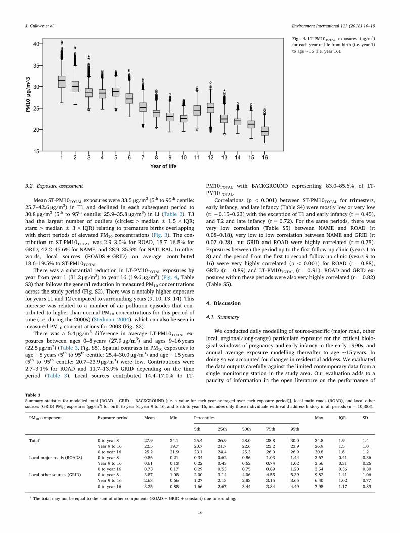
There was a substantial reduction in LT-PM10TOTAL exposures byyear from year 1 (31.2 μg/m3) to year 16 (19.6 μg/m3) (Fig. 4, TableS3) that follows the general reduction in measured PM10 concentrationsacross the study period (Fig. S2). There was a notably higher exposurefor years 11 and 12 compared to surrounding years (9, 10, 13, 14). Thisincrease was related to a number of air pollution episodes that con-tributed to higher than normal PM10 concentrations for this period oftime (i.e. during the 2000s) (Stedman, 2004), which can also be seen inmeasured PM10 concentrations for 2003 (Fig. S2).

There was a 5.4 μg/m3 difference in average LT-PM10TOTAL ex-posures between ages 0–8 years (27.9 μg/m3) and ages 9–16 years(22.5 μg/m3) (Table 3, Fig. S5). Spatial contrasts in PM10 exposures toage ~8 years (5th to 95th centile: 25.4–30.0 μg/m3) and age ~15 years(5th to 95th centile: 20.7–23.9 μg/m3) were low. Contributions were2.7–3.1% for ROAD and 11.7–13.9% GRID depending on the timeperiod (Table 3). Local sources contributed 14.4–17.0% to LT-

PM10TOTAL with BACKGROUND representing 83.0–85.6% of LT-PM10TOTAL.

Correlations (p < 0.001) between ST-PM10TOTAL for trimesters,early infancy, and late infancy (Table S4) were mostly low or very low(r: −0.15–0.23) with the exception of T1 and early infancy (r= 0.45),and T2 and late infancy (r= 0.72). For the same periods, there wasvery low correlation (Table S5) between NAME and ROAD (r:0.08–0.18), very low to low correlation between NAME and GRID (r:0.07–0.28), but GRID and ROAD were highly correlated (r= 0.75).Exposures between the period up to the first follow-up clinic (years 1 to8) and the period from the first to second follow-up clinic (years 9 to16) were very highly correlated (p < 0.001) for ROAD (r= 0.88),GRID (r= 0.89) and LT-PM10TOTAL (r= 0.91). ROAD and GRID ex-posures within these periods were also very highly correlated (r= 0.82)(Table S5).

4. Discussion

4.1. Summary

We conducted daily modelling of source-specific (major road, otherlocal, regional/long-range) particulate exposure for the critical biolo-gical windows of pregnancy and early infancy in the early 1990s, andannual average exposure modelling thereafter to age ~15 years. Indoing so we accounted for changes in residential address. We evaluatedthe data outputs carefully against the limited contemporary data from asingle monitoring station in the study area. Our evaluation adds to apaucity of information in the open literature on the performance of

Fig. 4. LT-PM10TOTAL exposures (μg/m3)for each year of life from birth (i.e. year 1)to age ~15 (i.e. year 16).

Table 3Summary statistics for modelled total [ROAD+GRID+BACKGROUND (i.e. a value for each year averaged over each exposure period)], local main roads (ROAD), and local othersources (GRID) PM10 exposures (μg/m3) for birth to year 8, year 9 to 16, and birth to year 16; includes only those individuals with valid address history in all periods (n=10,383).

PM10 component Exposure period Mean Min Percentiles Max IQR SD

5th 25th 50th 75th 95th

Totala 0 to year 8 27.9 24.1 25.4 26.9 28.0 28.8 30.0 34.8 1.9 1.4Year 9 to 16 22.5 19.7 20.7 21.7 22.6 23.2 23.9 26.9 1.5 1.00 to year 16 25.2 21.9 23.1 24.4 25.3 26.0 26.9 30.8 1.6 1.2

Local major roads (ROADS) 0 to year 8 0.86 0.21 0.34 0.62 0.86 1.03 1.44 3.67 0.41 0.36Year 9 to 16 0.61 0.13 0.22 0.43 0.62 0.74 1.02 3.56 0.31 0.260 to year 16 0.73 0.17 0.29 0.53 0.75 0.89 1.20 3.54 0.36 0.30

Local other sources (GRID) 0 to year 8 3.87 1.08 2.00 3.14 4.06 4.55 5.39 9.82 1.41 1.06Year 9 to 16 2.63 0.66 1.27 2.13 2.83 3.15 3.65 6.40 1.02 0.770 to year 16 3.25 0.88 1.66 2.67 3.44 3.84 4.49 7.95 1.17 0.89

a The total may not be equal to the sum of other components (ROAD+GRID+ constant) due to rounding.

J. Gulliver et al. Environment International 113 (2018) 10–19

16

models in predicting short-term exposures in the early 1990s. Exposureestimates will be used in a number of planned epidemiological studies.Data will be added to the ALSPAC resource for other users (http://www.bristol.ac.uk/alspac/researchers/).

4.2. Model performance

Our model estimates correlated well with weekly measured PM10

concentrations in Bristol for 1993, a period up to one year beyond thelast pregnancy in ALSPAC and overlapping early/late infancy for someof the cohort. We expected the mean bias (21%) to be lower for longeraveraging periods in our study (e.g. trimesters), but measurements ofPM10 concentrations were not sufficient to confirm this. Few otherstudies have evaluated the performance of PM10 dispersion modellingfor averaging periods of less than a year and we are not aware of anysuch studies for the 1990s. In Christchurch, New Zealand, dispersionmodelling was used to model daily concentrations of PM10 over twowinter months (July 2003 and June 2004) for 11 intra-urban sites(Wilson and Zawar-Reza, 2006). Absolute bias for the two-monthlyaverages was highly variable between sites (−33–44%) and mean biasfor the 11 sites was 31%. Srimath et al. (2017) combined models oflocal (CAR-FMI) and background (UK emissions model) PM10 in Londonand found strong correlation (r2= 0.68) between daily measured andpredicted PM10 concentrations at a single roadside site for 2008. Themodelling, however, under-estimated measured PM10 concentrationsby ~20%. Other studies used distance from residence to the nearestmajor road and local models to estimate traffic-related exposures forsome gaseous pollutants (e.g. NOX, NO2), but relied on average con-centration values from one monitoring site within each community asthe exposure for PM2.5 and PM10 (Heck et al., 2013; McConnell et al.,2010; Urman et al., 2014).

In general, model performance tends to be better for annual PM10

concentrations than it does for short-term PM10 concentrations (e.g.daily, weekly). Beevers et al. (2013), for example, using a combinationof a local model based on ADMS-Urban (KCL-Urban) and backgroundmodel (CMAQ) in London, reported very high correlation (r2= 0.96)and almost zero bias between measured and modelled PM10 for 2008,albeit with a relatively low number of sites (n= 12). Model perfor-mance in other studies has been good except where there is insufficientgranularity and/or coverage of local sources (Deutsch et al., 2008; deHoogh et al., 2014). We were unable to quantify the spatial bias in long-term exposures in ALSPAC as our evaluation was limited to a singlemonitoring site at any time (1993–2008).

4.3. Exposure contrasts

PM10 is a complex pollutant having both primary and secondarycontributions and a varied chemical composition and associatedsources. The coarse component (between 2.5 and 10 μm) of PM10 willgenerally be dominated by local sources, since the long-range coarsecontribution tends to sediment/deposit out during transport over longerdistances. The majority of the fine component (size < 2.5 μm) of PM10

tends to be secondary aerosol, formed from both local and distant gasphase precursors and transported on a regional scale. A relatively smalland direct (i.e. primary) contribution is from local sources. It followsthat the largest contribution (up to 46% of ST-PM10TOTAL) to exposuresduring pregnancy and early/late infancy was from the NAME compo-nent (Fig. S4). In our study local road sources (ROAD) made on averagethe smallest contribution to exposures (~3%) and the contribution oflocal other sources (GRID) was on average greater than ROAD by afactor of> 5 (~16% of total). In a mother-child (n= 1154) study of airpollution and birth weight in France (Rahmalia et al., 2012), local ex-posures modelled with ADMS-Urban represented (based on our inter-pretation of data presented in Table 1 of Rahmalia et al., 2012) about15% and 12% of total PM10 exposures in Nancy and Poitiers, respec-tively.

Intra-subject exposure contrasts over longer averaging periods (e.g.from birth to age 8 years) are related only to spatial variations in localsources of PM10, accounting for residential mobility, and were small inthis study. Similarly, other studies (Beevers et al., 2013; Carrutherset al., 2003) have shown that, although at some sites by main roadsPM10 concentrations were> 5 μg/m3 higher than those found in nearbybackground areas, at other main roads PM10 concentrations were only1–2 μg/m3 higher than nearby urban background sites. Air pollutiongradients can be steep in the wake of road sources, reaching back-ground levels at a variable distance (e.g. 20–100m) from source, whichis dependent on the street configuration and land cover between sourceand address (e.g. built-up area versus open-country); we studied this byrunning ADMS-Urban under different wind conditions (direction andspeed) and for a hypothetical main road of 500m in length with a dailyaverage traffic flow of 12,000 vehicles (40 km h−1), PM10 concentra-tions perpendicular to the road reduced on average by 4.8 μg/m3 from10m to 50m and by 5.6 μg/m3 from 10m to 100m. Air pollutiongradients are especially steep in the wake of some main roads. Differ-ences of> 10 μg/m3 for measurements of annual average PM10 havebeen shown between kerbside (within 1m of the kerb) and roadside(2–10m from the kerb) sites in the UK (Beevers et al., 2013; Carrutherset al., 2003). It is not surprising therefore that exposure contrasts be-tween subjects in ALSPAC, most of whom do not live close to mainroads (i.e. 9.5% of address locations are within 5–50m of a main road),were relatively small.

Fecht et al. (2016) separately assessed the contribution of roadtraffic and other sources to annual average (2003–2010) PM10 ex-posures for 190,122 postcodes (average of 12 households per postcode)in the area of Greater London. PM10 exposures from road traffic varied,depending on the year, between 2.9 μg/m3 and 3.5 μg/m3. This equatesto 11–15% of total PM10 exposures, which is a factor of 4–5 timeshigher than in our study in Bristol for an overlapping period(2003–2008). The Fecht et al. study was, however, conducted in amega-city of> 8 million residents, with a higher density of main roads(0.5 km/km2 in the ALSPAC study area compared to 3 km/km2 inGreater London), and 4 times the number (38.5%) of address locationswithin 50m of a main road than in our study area. Even though ourstudy and these studies are not directly comparable, due to differentlocations and time periods, we believe that exposure contrasts due tomain roads that we have estimated in ALSPAC are thus generally of thecorrect magnitude.

We found low correlations between pregnancy trimester and in-fancy exposures, which has been seen in the small number of otherstudies with information on both pregnancy trimester and early lifeexposures. For PM10, Van den Hooven et al. (2012), in the Generation Rstudy in The Netherlands, reported low to moderate correlation (r:0.31–0.48) between trimesters and low correlation between early andlate infancy (r= 0.21). We found moderate correlation between tri-mester 1 and early infancy and high correlation between trimester 2and late infancy. These periods overlap seasonally but their timing isnot a determinant of correlations per se, as elevated PM10 exposures innorth-western Europe, which are often related to low wind speeds andeasterly air flow, can happen throughout the year (Stedman, 2004). Forepidemiological studies interested in the effects of separate PM10 sourcecomponents, there was low correlation between NAME and local ex-posure components (ROAD+GRID), and high, but not very high,correlation between ROAD and GRID. Thus, although local sourcesmake up a relatively small proportion of total PM10, these correlationsindicate that local sources could have independence and be significantin epidemiological studies.

4.4. Limitations and strengths

Although we gathered a large amount of detailed information onlocal and non-local emissions sources and meteorological data to runthe dispersion models, our study has a number of limitations. We did

J. Gulliver et al. Environment International 113 (2018) 10–19

17

not have information on emissions from individual point sources (e.g.industrial stacks) as this was not available for the earlier years in thestudy period, so instead we used aggregated emissions information onall sources, except main roads, on a 1 km grid. This may mean that wehave under- or over-estimated the contribution of individual sources toPM10 concentrations. We were limited to using national-scale time-varying emissions factors as there is no information available on localfactors to cover the study period. Furthermore, we did not includeemissions of SO2 within the study area meaning that sulphate chemistry(i.e. the creation of secondary particulates by oxidising SO2 to formammonium sulphate) was not accounted for in modelling PM10 withADMS-Urban. This may have contributed to an underestimation of localsources of PM10 concentrations in some locations. In turn, this may alsomean that our values of background concentrations are too large as theywere determined by subtracting the sum of model estimates frommeasured concentrations of PM10.

We modelled dispersion of local sources of PM10 without accountingfor the effects of terrain or buildings. There are options to includeterrain and buildings in ADMS-Urban, but it was not practicable tomodel building effects over a large area as only 30 buildings could beincluded in a single model run of the version of ADMS-Urban that weused. We did not model the effects of terrain as this would have sub-stantially increased the run time of our models beyond what waspracticable. We recognize that although the study area is relatively flat,not including terrain in some locations may have contributed to errorsin our exposure estimates. We did not have enough information onrainfall to model wet deposition with ADMS-Urban, but we believe thisdid not greatly affect our exposure estimates as we averaged overperiods of at least a week for model evaluation and at least a trimesterwhen assigning exposures.

We applied a single constant of 12 μg/m3 that was imputed fromlimited (1993) measured PM10 concentrations in the study area, to re-present local ‘natural’ sources in estimates of ST-PM10TOTAL. In realitythis will vary over time depending on meteorology, but we are unableto account for this during the pregnancy and early life period as weneeded exposure estimates for periods prior to 1993 when there was noPM10 monitoring within the study area. A value of 12.0 μg/m3 is ap-proximately the 1st centile of measured PM10 concentrations from 1993at the Bristol Centre site; thus we believe it to be of the correct mag-nitude to represent an average PM10 concentration without the pre-sence of local anthropogenic source. We imputed yearly constants fromtwo monitoring sites in the centre of Bristol to represent ‘background’PM10 (i.e. natural sources and regional/long-range aerosol from outsidethe study area). These may contribute to over-estimating backgroundLT-PM10 concentrations for other locations, but there was no othermonitoring of PM10 in the study area at any time. The nearest rural site(Narberth, Wales) was operational from 1997, but being 140 km to thewest raises doubts about its representativeness of background con-centrations for Avon.

Despite these limitations we have produced detailed exposuremodels from conception through to age 15 years (1990–2008) for dif-ferent critical life periods, using a methodology where we are able toseparately quantify local and non-local sources of PM10 for epidemio-logical investigations. It is a strength of the study that we were able toundertake model evaluation for exposure periods overlapping withpregnancy and early life in the early 1990s. A further strength is that wewere able to account for residential mobility over the whole studyperiod for a large proportion of ALSPAC participants.

Funding

The research was supported by The UK Medical Research Council/Wellcome Trust (Grant ref.: 102215/2/13/2), the University of Bristolprovide core support for ALSPAC. The work of the UK Small AreaHealth Statistics Unit is funded by Public Health England as part of theMRC-PHE Centre for Environment and Health, funded also by the UK

Medical Research Council (Grant ref.: MR/L01341X/1). This paper doesnot necessarily reflect the views of Public Health England or theDepartment of Health.

Acknowledgements

We are extremely grateful to all the families who took part in thisstudy, the midwives for their help in recruiting them, and the wholeALSPAC team, which includes interviewers, computer and laboratorytechnicians, clerical workers, research scientists, volunteers, managers,receptionists and nurses. The UK Medical Research Council and theWellcome Trust (Grant ref.: 102215/2/13/2) and the University ofBristol provide core support for ALSPAC. This publication is the work ofthe authors and John Gulliver, Paul Elliott, and John Henderson willserve as guarantors for the contents of this paper. This research wasspecifically funded by The UK Medical Research Council: “Effects OfEarly Life Exposure To Particulates On Respiratory Health ThroughChildhood And Adolescence: ALSPAC Birth Cohort Study”, Grant Ref:G0700920. We thank Bristol City Council for providing data on trafficflows/speeds and emission rates for the ALSPAC study area. Paul Elliottacknowledges support of the NIHR Biomedical Research Centre atImperial College Healthcare NHS Trust and Imperial College London,and the NIHR Health Protection Research Unit in Health Impact ofEnvironmental Hazards (HPRU-2012-10141). Yutong Cai acknowledgessupport from the Early-Career Research Fellowship awarded by the UKMedical Research Council–Public Health England Centre forEnvironment and Health (Grant number MR/M501669/1).

Appendix A. Supplementary data

Supplementary data to this article can be found online at https://doi.org/10.1016/j.envint.2018.01.017.

References

Atkinson, R.W., Carey, I.M., Kent, A.J., van Staa, T.P., Anderson, H.R., Cook, D.G., 2015.Long-term exposure to outdoor air pollution and the incidence of chronic obstructivepulmonary disease in a national English cohort. Occup. Environ. Med. 72 (1), 42–48.

Baiz, N., Dargent-Molina, P., Wark, J.D., Souberbielle, J.C., Slama, R., Annesi-Maesano, I.,EDEN Mother-Child Cohort Study Group, 2012. Gestational exposure to urban airpollution related to a decrease in cord blood vitamin d levels. J. Clin. Endocrinol.Metab. 97 (11), 4087–4095.

Beevers, S.D., Kitwiroon, N., Williams, M.L., Kelly, F.J., Ross Anderson, H., Carslaw, D.C.,2013. Air pollution dispersion models for human exposure predictions in London. J.Expo. Sci. Environ. Epidemiol. 23 (6), 647–653.

Bellander, T., Berglind, N., Gustavsson, P., Jonson, T., Nyberg, F., Pershagen, G., Jarup,L., 2001. Using geographic information systems to assess individual historical ex-posure to air pollution from traffic and house heating in Stockholm. Environ. HealthPerspect. 109 (6), 633–639.

Bennett, N.D., Croke, B.F.W., Guariso, G., Guillaume, J.H.A., Hamilton, S.H., Jakeman,A.J., Marsili-Libelli, S., Newham, L.T.H., Norton, J.P., Perrin, C., Pierce, S.A., Robson,B., Seppelt, R., Voinov, A.A., Fath, B.D., Andreassian, V., 2013. Characterising per-formance of environmental models. Environ. Model. Softw. 40, 1–20.

Berrisford, P., et al., 2011. The ERA-Interim archive version 2.0. In: ERA Report Series 1.ECMWF, Shinfield Park, Reading, UK, pp. 13177.

Boyd, A., Golding, J., Macleod, J., Lawlor, D.A., Fraser, A., Henderson, J., Molloy, L.,Ness, A., Ring, S., Davey Smith, G., 2013. Cohort Profile: the ‘children of the90s’—the index offspring of the Avon Longitudinal Study of Parents and Children. Int.J. Epidemiol. 42 (1), 111–127.

Brunst, K.J., Ryan, P.H., Brokamp, C., Bernstein, D., Reponen, T., Lockey, J., KhuranaHershey, G.K., Levin, L., Grinshpun, S.A., LeMasters, G., 2015. Timing and durationof traffic-related air pollution exposure and the risk for childhood wheeze andasthma. Am. J. Respir. Crit. Care Med. 192 (4), 421–427.

Bush, T., Smith, S., Stevenson, K., Moorcroft, S., 2001. Validation of nitrogen dioxidediffusion tube methodology in the UK. Atmos. Environ. 35 (2), 289–296.

Butland, B.K., Atkinson, R.W., Crichton, S., Barratt, B., Beevers, S., Spiridou, A., Hoang,U., Kelly, F.J., Wolfe, C.D., 2017. Air pollution and the incidence of ischaemic andhaemorrhagic stroke in the South London Stroke Register: a case-cross-over analysis.J. Epidemiol. Community Health 71 (7), 707–712.

Carruthers, D.J., Holroyd, R.J., Hunt, J.C.R., Weng, W.-S., Robins, A.G., Apsley, D.D.,Thompson, D.J., Smith, F.B., 1994. UK-ADMS-Urban: a new approach to modellingdispersion in the earth's atmospheric boundary layer. J. Wind Eng. Ind. Aerodyn. 52,139–153. http://dx.doi.org/10.1016/0167-6105(94)90044-2.

Carruthers, D.J., Blair, K., Johnson, K., 2003. Validation and sensitivity of ADMS-Urban-Urban for London Cambridge Environmental Research Consultants: TR0191. https://

J. Gulliver et al. Environment International 113 (2018) 10–19

18

uk-air.defra.gov.uk/assets/documents/reports/cat09/Validation&Sensitivity(22JAN03)10_TR-0191-h.pdf, Accessed date: 31 July 2017.

Charpin, D., Penard-Morand, C., Raherison, C., Kopferschmitt, C., Lavaud, F., Caillaud, D.,Annesi-Maesano, I., 2009. Long-term exposure to urban air pollution measuredthrough a dispersion model and the risk of asthma and allergy in children. Bull. Acad.Natl Med. 193 (6), 1317–1328 (discussion 1328–9).

Deutsch, F., Mensink, C., Vankerkom, J., Janssen, L., 2008. Application and validation ofa comprehensive model for PM10 and PM2.5 concentrations in Belgium and Europe.Appl. Math. Model. 32 (8), 1501–1510.

Fecht, D., Hansell, A.L., Morley, D., Dajnak, D., Vienneau, D., Beevers, S., Toledano, M.B.,Kelly, F.J., Anderson, H.R., Gulliver, J., 2016. Spatial and temporal associations ofroad traffic noise and air pollution in London: implications for epidemiological stu-dies. Environ. Int. 88, 235–242.

Fuertes, E., Standl, M., Cyrys, J., Berdel, D., von Berg, A., Bauer, C.P., Kramer, U., Sugiri,D., Lehmann, I., Koletzko, S., Carlsten, C., Brauer, M., Heinrich, J., 2013. A long-itudinal analysis of associations between traffic-related air pollution with asthma,allergies and sensitization in the GINIplus and LISAplus birth cohorts. PeerJ 1, e193.

Fuertes, E., Bracher, J., Flexeder, C., Markevych, I., Klumper, C., Hoffmann, B., Kramer,U., von Berg, A., Bauer, C.P., Koletzko, S., Berdel, D., Heinrich, J., Schulz, H., 2015.Long-term air pollution exposure and lung function in 15 year-old adolescents livingin an urban and rural area in Germany: the GINIplus and LISAplus cohorts. Int. J.Hyg. Environ. Health 218 (7), 656–665.

Wilson, J.G., Zawar-Reza, P., 2006. Intraurban-scale dispersion modelling of particulatematter concentrations: applications for exposure estimates in cohort studies. Atmos.Environ. 40 (6), 1053–1063.

Gauderman, W.J., Urman, R., Avol, E., Berhane, K., McConnell, R., Rappaport, E., Chang,R., Lurmann, F., Gilliland, F., 2015. Association of improved air quality with lungdevelopment in children. N. Engl. J. Med. 372 (10), 905–913.

Gehring, U., Wijga, A.H., Hoek, G., Bellander, T., Berdel, D., Bruske, I., Fuertes, E.,Gruzieva, O., Heinrich, J., Hoffmann, B., de Jongste, J.C., Klumper, C., Koppelman,G.H., Korek, M., Kramer, U., Maier, D., Melen, E., Pershagen, G., Postma, D.S., Standl,M., von Berg, A., Anto, J.M., Bousquet, J., Keil, T., Smit, H.A., Brunekreef, B., 2015.Exposure to air pollution and development of asthma and rhinoconjunctivitisthroughout childhood and adolescence: a population-based birth cohort study. LancetRespir. Med. 3 (12), 933–942.

Gong, T., Dalman, C., Wicks, S., Dal, H., Magnusson, C., Lundholm, C., Almqvist, C.,Pershagen, G., 2017. Perinatal exposure to traffic-related air pollution and autismspectrum disorders. Environ. Health Perspect. 125 (1), 119–126.

Hampel, R., Lepeule, J., Schneider, A., Bottagisi, S., Charles, M.A., Ducimetiere, P., Peters,A., Slama, R., 2011. Short-term impact of ambient air pollution and air temperatureon blood pressure among pregnant women. Epidemiology 22 (5), 671–679.

Hansen, A.B., Ravnskjaer, L., Loft, S., Andersen, K.K., Brauner, E.V., Baastrup, R., Yao, C.,Ketzel, M., Becker, T., Brandt, J., Hertel, O., Andersen, Z.J., 2016. Long-term ex-posure to fine particulate matter and incidence of diabetes in the Danish NurseCohort. Environ. Int. 91, 243–250.

Heck, J.E., Wu, J., Lombardi, C., Qiu, J., Meyers, T.J., Wilhelm, M., Cockburn, M., Ritz,B., 2013. Childhood cancer and traffic-related air pollution exposure in pregnancyand early life. Environ. Health Perspect. 121 (11-12), 1385–1391.

de Hoogh, K., Korek, M., Vienneau, D., Keuken, M., Kukkonen, J., Nieuwenhuijsen, M.J.,Badaloni, C., Beelen, R., Bolignano, A., Cesaroni, G., Pradas, M.C., Cyrys, J., Douros,J., Eeftens, M., Forastiere, F., Forsberg, B., Fuks, K., Gehring, U., Gryparis, A.,Gulliver, J., Hansell, A.L., Hoffmann, B., Johansson, C., Jonkers, S., Kangas, L.,Katsouyanni, K., Kunzli, N., Lanki, T., Memmesheimer, M., Moussiopoulos, N.,Modig, L., Pershagen, G., Probst-Hensch, N., Schindler, C., Schikowski, T., Sugiri, D.,Teixido, O., Tsai, M.Y., Yli-Tuomi, T., Brunekreef, B., Hoek, G., Bellander, T., 2014.Comparing land use regression and dispersion modelling to assess residential ex-posure to ambient air pollution for epidemiological studies. Environ. Int. 73,382–392.

Hsu, H.H., Chiu, Y.H., Coull, B.A., Kloog, I., Schwartz, J., Lee, A., Wright, R.O., Wright,R.J., 2015. Prenatal particulate air pollution and asthma onset in urban children.Identifying sensitive windows and sex differences. Am. J. Respir. Crit. Care Med. 192(9), 1052–1059.

Jones, A.R., Thomson, D.J., Hort, M., Devenish, B., 2007. The U.K. Met Office's next-generation atmospheric dispersion model, NAME III. In: Borrego, C., Norman, A.-L.(Eds.), Air Pollution Modeling and Its Application XVII (Proceedings of the 27thNATO/CCMS International Technical Meeting on Air Pollution Modelling and ItsApplication). Springer, pp. 580–589.

Keuken, M., Zandveld, P., van den Elshout, S., Janssen, N.A.H., Hoek, G., 2011. Airquality and health impact of PM10 and EC in the city of Rotterdam, the Netherlandsin 1985–2008. Atmos. Environ. 45 (30), 5294–5301.

Korek, M.J., Bellander, T.D., Lind, T., Bottai, M., Eneroth, K.M., Caracciolo, B., de Faire,U.H., Fratiglioni, L., Hilding, A., Leander, K., Magnusson, P.K., Pedersen, N.L.,Ostenson, C.G., Pershagen, G., Penell, J.C., 2015. Traffic-related air pollution ex-posure and incidence of stroke in four cohorts from Stockholm. J. Expo. Sci. Environ.Epidemiol. 25 (5), 517–523.

McConnell, R., Islam, T., Shankardass, K., Jerrett, M., Lurmann, F., Gilliland, F.,Gauderman, J., Avol, E., Kunzli, N., Yao, L., Peters, J., Berhane, K., 2010. Childhoodincident asthma and traffic-related air pollution at home and school. Environ. HealthPerspect. 118 (7), 1021–1026.

Molter, A., Simpson, A., Berdel, D., Brunekreef, B., Custovic, A., Cyrys, J., de Jongste, J.,de Vocht, F., Fuertes, E., Gehring, U., Gruzieva, O., Heinrich, J., Hoek, G., Hoffmann,B., Klumper, C., Korek, M., Kuhlbusch, T.A., Lindley, S., Postma, D., Tischer, C.,Wijga, A., Pershagen, G., Agius, R., 2015. A multicentre study of air pollution ex-posure and childhood asthma prevalence: the ESCAPE project. Eur. Respir. J. 45 (3),610–624.

Morales, E., Garcia-Esteban, R., de la Cruz, O.A., Basterrechea, M., Lertxundi, A., deDicastillo, M.D., Zabaleta, C., Sunyer, J., 2015. Intrauterine and early postnatal ex-posure to outdoor air pollution and lung function at preschool age. Thorax 70 (1),64–73.

Mortimer, K., Neugebauer, R., Lurmann, F., Alcorn, S., Balmes, J., Tager, I., 2008. Airpollution and pulmonary function in asthmatic children: effects of prenatal andlifetime exposures. Epidemiology 19 (4), 550–557 (discussion 561-2).

Nordling, E., Berglind, N., Melen, E., Emenius, G., Hallberg, J., Nyberg, F., Pershagen, G.,Svartengren, M., Wickman, M., Bellander, T., 2008. Traffic-related air pollution andchildhood respiratory symptoms, function and allergies. Epidemiology 19 (3),401–408.

Pirani, M., Gulliver, J., Fuller, G.W., Blangiardo, M., 2014. Bayesian spatiotemporalmodelling for the assessment of short-term exposure to particle pollution in urbanareas. J. Expo. Sci. Environ. Epidemiol. 24 (3), 319–327.

Rahmalia, A., Giorgis-Allemand, L., Lepeule, J., Philippat, C., Galineau, J., Hulin, A.,Charles, M.A., Slama, R., EDEN Mother-Child Cohort Study group, 2012. Pregnancyexposure to atmospheric pollutants and placental weight: an approach relying on adispersion model. Environ. Int. 48, 47–55.

Rice, M.B., Rifas-Shiman, S.L., Litonjua, A.A., Oken, E., Gillman, M.W., Kloog, I.,Luttmann-Gibson, H., Zanobetti, A., Coull, B.A., Schwartz, J., Koutrakis, P.,Mittleman, M.A., Gold, D.R., 2016. Lifetime exposure to ambient pollution and lungfunction in children. Am. J. Respir. Crit. Care Med. 193 (8), 881–888.

Sbihi, H., Tamburic, L., Koehoorn, M., Brauer, M., 2016. Perinatal air pollution exposureand development of asthma from birth to age 10 years. Eur. Respir. J. 47 (4),1062–1071.

Schultz, E.S., Hallberg, J., Pershagen, G., Melen, E., 2016. Reply: early-life exposure totraffic-related air pollution and lung function in adolescence. Am. J. Respir. Crit. CareMed. 194 (3), 385–386.

Sellier, Y., Galineau, J., Hulin, A., Caini, F., Marquis, N., Navel, V., Bottagisi, S., Giorgis-Allemand, L., Jacquier, C., Slama, R., Lepeule, J., 2014. Health effects of ambient airpollution: do different methods for estimating exposure lead to different results?Environ. Int. 66, 165–173.

Srimath, S.T.G., Sokhi, R., Karppinen, A., Singh, V., Kukkonen, J., 2017. Evaluation of anurban modelling system against three measurement campaigns in London andBirmingham. Atmos. Pollut. Res. 8 (1), 38–55.

Stedman, J.R., 2004. The predicted number of air pollution related deaths in the UKduring the August 2003 heatwave. Atmos. Environ. 38 (8), 1087–1090.

Urman, R., McConnell, R., Islam, T., Avol, E.L., Lurmann, F.W., Vora, H., Linn, W.S.,Rappaport, E.B., Gilliland, F.D., Gauderman, W.J., 2014. Associations of children'slung function with ambient air pollution: joint effects of regional and near-roadwaypollutants. Thorax 69 (6), 540–547.

Van den Hooven, E.H., Pierik, F.H., Van Ratingen, S.W., Zandveld, P.Y., Meijer, E.W.,Hofman, A., Miedema, H.M., Jaddoe, V.W., De Kluizenaar, Y., 2012. Air pollutionexposure estimation using dispersion modelling and continuous monitoring data in aprospective birth cohort study in The Netherlands. Environ. Health 11, 9.

Vinceti, M., Malagoli, C., Malavolti, M., Cherubini, A., Maffeis, G., Rodolfi, R., Heck, J.E.,Astolfi, G., Calzolari, E., Nicolini, F., 2016. Does maternal exposure to benzene andPM10 during pregnancy increase the risk of congenital anomalies? A population-based case-control study. Sci. Total Environ. 541, 444–450.

J. Gulliver et al. Environment International 113 (2018) 10–19

19