Local and Duration Magnitudes in Northwestern Italy, … 44N29.48 10E0395 0.87 Lennartz LE3D-5s (3C)...

592

Bulletin of the Seismological Society of America, Vol. 95, No. 2, pp. 592–604, April 2005, doi: 10.1785/0120040099

Local and Duration Magnitudes in Northwestern Italy, and Seismic Moment

Versus Magnitude Relationships

by D. Bindi, D. Spallarossa, C. Eva, and M. Cattaneo

Abstract In the present work, we develop some local magnitude scales for north-western Italy based on vertical short-period records. This study is motivated by thepossibility of applying the computed scales to an instrumental catalog of more than25,000 local earthquakes, as this region has been continuously monitored by 12 short-period vertical-component (1C) stations since the mid-1980s. Furthermore, a digitalnetwork of three-component (3C) broadband or 5 second sensors has monitorednorthwestern Italy since 1996. Today, a significant number of earthquakes have beensimultaneously recorded by both networks, allowing the calibration of the 1C localscale by using magnitudes computed according to a scale derived for the 3C digitalnetwork. Moreover, because station Sant’ Anna di Valdieri houses both a 3C (codeSTV2) and 1C (code STV) sensors, the magnitude scales for the two networks can bedeveloped using the same reference station. The magnitude scale ML � log A �log(R/100) � 0.0054(R � 100) � 3 � S is derived for the 3C digital network withthe requirement that the correction S of station STV2 is zero. This scale is based on10,057 maximum amplitudes (2822 earthquakes) computed from horizontal synthe-sized Wood-Anderson seismograms, in the hypocentral distance 10 to 310 km andin the range 0 � ML � 5. With respect to an carlier magnitude scale derived for the3C network constraining the sum of all the station corrections to zero, the magnitudespredicted by the previous equations show an average bias of (�0.2 � 0.1), whichcan be ascribed to the different constraint applied to the station corrections. Themagnitudes predicted by the scale for the 3C network are used to calibrate magnitudescales based on either total duration or maximum amplitude from synthesized Wood-Anderson seismograms computed for each short-period vertical recording. The mag-nitude scale obtained considering maximum amplitudes from vertical short-periodrecordings is ML � log A � log(R/100) � 0.0041 (R � 100) � 3 � S�. Thereliability of the obtained magnitude scales is assessed using 827 earthquakes dif-ferent from those we considered in the regression analysis. Finally, the followingseismic moment versus local magnitude relations are valid in the western Alps in therange 0 � ML � 4.5:

3Clog M � (0.92 � 0.01) M � (17.38 � 0.08)0 L1Clog M � (0.95 � 0.01) M � (17.36 � 0.01)0 L

where ML3C is the local magnitude computed starting from the horizontal component

of broadband (flat frequency response, from 0.033 to 50 Hz) or semibroadband (flatfrequency response, from 0.2 to 40 Hz) sensors and ML

1C is the magnitude computedstarting from the vertical short-period recordings.

Introduction

Northwestern Italy is characterized by small to moder-ate seismicity (ML � 3), and about two earthquakes of mag-nitude greater than 4.5 are expected each year (Spallarossa

et al., 2002). The recent largest earthquakes occurred on 21August 2000 (Asti, ML 4.8), on 18 July 2001 (Asti, ML 4.6),and on 11 April 2003 (Novi Ligure, ML 4.8). Seismogenic

Local and Duration Magnitudes in Northwestern Italy, and Seismic Moment Versus Magnitude Relationships 593

structures able to generate a damaging earthquake are alsopresent in this area. For example, the 1887, Ms 6.4 Bussanaearthquake (Capponi et al., 1985) that occurred in westernLiguria, and the 1920, Ms 6.5 Lunigiana-Garfagnana earth-quake (Ferrari et al., 1985) that occurred in the northernApennines caused significant damage and casualities. Since1982, the RSNI/RSGL (Regional Seismic network of north-western Italy, formerly the IGG network) has monitoredseismicity in the western Alps and in the Ligurian sea and,since 1998, in the northern Apennines (Cattaneo and Aug-liera, 1990; Solarino et al., 1997; Cattaneo et al., 1999; Evaet al., 2001; Solarino et al., 2002). Furthermore, the north-western Alps are contained in the area monitored by severalseismological observatories (Laboratoire de Detection et deGeophysique [LDG/CEA], Bruyeres-le-Chatel, Frances;Swiss Seismological Service [SSS], Zurich, Switzerland; La-boratoire de Geophysique Interne et Tectonophysique [SIS-MALP], Grenoble, France; Reseau National de SurveillanceSismique [ReNaSS], Strasburg, France; Instituto Nazionaledi Geofisica e Vulcanologia [INGV], Rome, Italy). To exploitthe possibility of merging the catalog provided by the dif-ferent networks, it is necessary to avoid inconsistencies inthe method adopted to compute the considered parametersand to clearly state how the shared quantities were com-puted. An example is the magnitude, which is the parameterusually adopted for first-cut reconnaissance analysis ofearthquake data for various geophysical and engineering in-vestigations (Kanamori, 1983). Moreover, in general, mag-nitude is the only information about the size of the earth-quake that spreads to the nonscientific community.Furthermore, magnitude catalogs are often subject of statis-tical analysis aimed at evaluating the seismic activity and atassessing the hazard of the considered area.

Several magnitude scales can be determined, based onamplitude measurements of different seismic phases or onthe total signal duration. As pointed out in the IASPEI NewManual of Seismological Observatory (Bormann, 2002, p.18), “there is no single number parameter available whichcould serve as a good estimate of earthquake size in all itsdifferent aspects.” The local magnitude ML (Richter, 1935,1958) from actual or synthesized Wood-Anderson amplitude(Uhrhammer and Collins, 1990) is a good measure of earth-quake size in terms of energy release and a good measure tospecify seismic hazard. The major limitation to its applica-bility is the saturation that takes place for strong earthquakes,leading ML to never exceed 7 (Kanamori, 1983, figure 4).The moment magnitude MW, being proportional to the staticaverage displacement and to the area of the fault, providesa measure of the total deformation in the source region anddoes not saturate for large earthquakes. In many seismolog-ical observatories that managed analog seismic networkscharacterized by short-period and low-dynamic equipment,magnitude scales based on total signal duration were devel-oped. The magnitudes MD reported in the RSNI bulletin(www.dipteris.unige.it/geofisica) are determined from thetotal signal duration visually estimated considering record-

ings from one-component, short-period stations. For eachstation, a MD scale was calibrated in the early 1980s by usingthe magnitude reported in the LDG network bulletin, withno distance correction (Cattaneo et al., 1981). More than 20years of seismological observations in the western Alpsdemonstrated the reliability and stability of this durationscale in the magnitude range from 2 to 4 MD, whereas, asshown in a work by Spallarossa et al. (2002, hereafter re-ferred to as SP-02), this scale overestimates magnitudes be-low ML 1.5 and underestimates magnitudes greater than 4.The overall goal of this study is the development of a reliablemagnitude scale based on maximum amplitude from verticalshort-period records that will allow us to compute a homo-geneous magnitude catalog suitable for seismotectonic andhazard studies. SP-02 calibrated a local magnitude scale forthe 3C network from synthesized Wood-Anderson seismo-grams, constraining the sum of all the station corrections tozero. To have the same reference for both the 3C and theshort-period networks, a new 3C magnitude calibration isperformed by imposing a different constraint over the stationcorrections. In particular, as station Sant’Anna di Valdierihouses both a 3C and a 1C sensor (code STV and STV2 forthe 1C and 3C sensors, respectively), new coefficients for theML scale from 3C recordings are computed by setting to zerothe station correction of STV2 alone. Then, regression anal-yses are carried out to derive new magnitude scales, basedon duration and amplitude measurements from short-periodinstruments. Finally, exploiting an available dataset of seis-mic moment Mo (Morasca et al., 2005), a comparison be-tween ML and log Mo is discussed.

Network and Data

The RSNI-Regional Seismic network of northwesternItaly arises from the integration of a regional network oftelemetered short-period stations (formerly, IGG network)with a network of digital stations equipped with three-component (3C) sensors (Table 1). Signals from the 12 one-component (1C) short-period stations are transmitted by fre-quency modulation via telephone line to the Data-ProcessingCentre in Genoa, managed by DipTeRis (Dipartimento perlo studio del Territorio e delle sue Risorse). The transmissionintroduces a dynamic range limitation (about 66 dB) and abandwidth reduction (0.2 to 25 Hz). At the Data-ProcessingCentre, signals are continuously digitized by a high-dynamicsystem and radio-synchronized to a DCF (German longwave signal Frankfurt) time signal. The 18 digital 3C stationsare equipped with either Lennartz LE3D-5s sensors (flat fre-quency response from 0.2 to 40 Hz) or Guralp CMG40 sen-sors (flat frequency response from 0.033 to 50 Hz). The ac-quisition is performed by a dial-up LennartzMars88 MCsystem provided with a 20-bit A/D converter. Table 1 pres-ents the main characteristics of the stations used in this work.Figure 1 shows the station locations and the local earth-quakes recorded from 1996 to 2003. A detailed description

594 D. Bindi, D. Spallarossa, C. Eva, and M. Cattaneo

Table 1Stations Used in This Study

Code Latitude LongitudeHeight(km) Sensor Type

Since(mm/yyyy)

BACM 44N16.70 10E04.33 0.49 Lennartz LE3D-5s (3C) 11/1998CODM 44N23.45 09E51.00 0.35 Lennartz LE3D-5s (3C) 03/1999FENE 45N01.81 07E03.76 1.00 Guralp CMG3 (3C) 10/1996GENL 44N24.34 08E58.18 0.08 Guralp CMG40 (3C) 01/1996GRAM 44N29.48 10E0395 0.87 Lennartz LE3D-5s (3C) 04/1999MAIM 43N54.85 10E29.49 0.20 Lennartz LE3D-5s (3C) 09/2000MONE 44N04.77 07E45.30 1.32 Guralp CMG40 (3C) 02/1995NEGI 43N50.86 07E42.23 0.64 Guralp CMG40 (3C) 03/1996RONM 43N54.88 07E35.89 0.30 Guralp CMG3 (3C) 01/1999RORM 44N52.88 07E35.89 0.30 Guralp CMG3 (3C) 03/2001ROTM 44N50.96 08E21.16 0.22 Lennartz LE3D-5s (3C) 07/2001SARM 44N11.05 10E24.06 1.04 Lennartz LE3D-5s (3C) 03/1998SCUM 44N24.98 09E32.23 0.75 Lennartz LE3D-5s (3C) 11/1998SESM 44N13.91 10E46.42 1.02 Lennartz LE3D-1s (3C) 07/2002STV2 44N14.73 07E19.56 0.93 Guralp CMG40 (3C) 10/1996TRAV 45N30.76 07E44.82 0.99 Guralp CMG40 (3C) 09/1996VALM 44N20.94 10E14.83 0.79 Lennartz LE3D-5s (3C) 03/1999VINM 44N08.47 10E0913 0.71 Lennartz LE3D-5s (3C) 10/1998ROB 44N17.75 07E53.18 0.81 Geotech S13 (1C) 06/1985BLB 44N50.11 07E15.80 0.58 Geotech S13 (1C) 05/1990ENR 44N13.77 07E25.10 1.03 Geotech S13 (1C) 05/1989FIN 44N12.49 08E12.53 0.60 Geotech S13 (1C) 06/1984IMI 43N54.63 07E53.59 0.84 Geotech S13 (1C) 11/1983LSD 45N27.57 07E08.06 2.28 Geotech S13 (1C) 10/1985ORX 45N37.90 07E58.90 1.23 Kinemetrics SS1 (1C) 12/1984PCP 44N32.48 08E32.71 0.77 Geotech S13 (1C) 03/1989PZZ 44N30.41 07E06.9 1.43 Kinemetrics SS1 (1C) 06/1985RRL 44N55.25 06E47.45 2.13 Kinemetrics SS1 (1C) 06/1985RSP 45N08.89 07E15.92 1.28 Geotech S13 (1C) 06/1985STV 44N14.73 07E19.56 0.93 Geotech S13 (1C) 12/1985

of the detection capabilities and location accuracy of theRSNI network can be found in Spallarossa et al. (2001).

In the present study, we selected earthquakes with epi-centers inside the investigated region (Fig. 1), azimuthal gapless than 220 degrees, and statistical horizontal and verticallocation errors (Lee and Lahr, 1975) less than 10 and 20 km,respectively. In all, 4832 earthquakes occurring from 1996to 2003 are part of the analyzed dataset.

Ml Calibration Using Three-Component (3C)Recordings

Data recorded from 1999 to 2003 are used to computea local magnitude scale using synthetic Wood-Anderson am-plitudes obtained from the horizontal component of 3C re-cordings. We calibrate a ML scale (Richter, 1935, 1958) fol-lowing the Bakun and Joyner (1984) parametric approach:

M � log A � n log(R/100)L

� k(R � 100) � 3 � S , (1)

where A is the observed maximum amplitude of the hori-zontal Wood-Anderson seismogram, n and k are attenuationcoefficients, S is a station correction, and R is the hypocentral

distance. The 1-mm amplitude constraint for a magnitude 3recorded at distance R � 100 km is applied. If amplitudesfrom seismometers different from the Wood-Anderson arehandled, it is a common practice (Uhrhammer and Collins,1990) to compute synthetic Wood-Anderson seismogramsby convolving the displacement corrected for instrumentalresponse with the Wood-Anderson torsion seismograph re-sponse. We use T0 � 0.8 sec, h � 0.8, and V � 2800 todescribe the Wood-Anderson response, consistently withmost of the local magnitude studies that adopted this valuefor the static magnification V instead of the correct value of2080 (Uhrhammer and Collins, 1990). To avoid amplifica-tion of the noise at low frequency, the instrument correctionand the Wood-Anderson convolution are performed in a fre-quency band for which the signal-to-noise ratio is greaterthan 5.

A local magnitude scale was calibrated for the 3C net-work by SP-02 using synthesized Wood-Anderson seismo-grams and constraining the sum of all the station correctionsto zero. To have the same reference for both the 3C and theshort-period networks, a new 3C magnitude calibration isperformed by setting to zero the correction of station STV2alone. The constraint applied to the station corrections intro-duces a dependence of the calibrated scale on the assumption


Figure 1. Seismicity recorded in the northwestern Alps and northern Apennines bythe RSNI network from 1996 to 2003. Triangles and squares indicate three-component(3C) and one-component (1C) stations, respectively. Station STV/STV2 is indicated bya star. Duration magnitude is taken from RSNI weekly bulletins.

made about the reference station. Because the magnitude ofan earthquake is generally computed as the average of themagnitudes estimated from the maximum amplitude ob-served at several stations, from equation (1) it follows:

NN 11 iM � M �L � L �N Ni�1 i�1

i i i(log A � n log(R / 100) � k(R � 100) � 3)

(2)N

1 i� S�N i�1

where the index i � 1, . . .,N spans the stations that recordedthe earthquake. Although the second term of the right handside of equation (2) was set to zero in SP-02, it is differentfrom zero in the present calibration. From equation (2) itfollows that the average magnitudes computed in this studywill differ from those computed from SP-02 by an offset

equal to the second term of the right hand side, that is, thearithmetic mean of the station corrections estimated in thisstudy.

The calibration is performed by considering 10,057 am-plitudes from 2822 earthquakes recorded at 18 stations, inthe range of distances from 10 to 310 km and following thesame procedure described in SP-02. Only the earthquakesoccurring from 1999 to 2003 are accounted for in this cali-bration. Figure 2 shows the locations of the earthquakes usedto calibrate the scale, the relative path coverage, the distri-bution in distance of the recordings, and the histogram ofthe horizontal location errors. Because a trade-off betweenthe geometrical spreading parameter n and the anelastic at-tenuation parameter k exists (Bakun and Joyner, 1984; Lang-ston et al., 1998), we perform the inversion constrainingn � 1. The linear system is solved in a least-squares senseby applying the LSQR technique (algorithm for sparse linearequations and sparse least squares) (Paige and Saunders,1982). The station corrections and the attenuation coefficient


Figure 2. Ray paths between events (circles) and stations (triangles) used in the 3Clocal magnitude calibration and the histograms of the distance distribution (left bottompanel) and horizontal location error (right bottom panel).

k are estimated by computing the mean and the standarddeviation of the distributions resulting from the inversion of200 bootstrap replications of the original dataset (Efron,1979; Spallarossa et al., 2002; Baumbach et al., 2003). Theinversion yielded k � (0.0054 � 0.0003). The station cor-rections (Table 2) vary in the range (�0.13 � 0.06) to (0.57� 0.04), whereas the magnitudes are in the range 0 to 5.Figure 3 (left) shows the magnitudes computed in this study

versus the magnitudes obtained by SP-02. Because the dif-ferences between the attenuation curves are negligible (Fig.3, right), the average difference of (�0.2 � 0.1) betweenthe magnitudes computed in this study and those computedby SP-02 is in good agreement with the value 0.18 expectedfrom equation (2) by using the station corrections listed inTable 2.

A peculiarity of the magnitude calibration scheme is the


Table 2Number of Earthquakes (#) Used to Calibrate the ML

3C MagnitudeScale and the Resulting Station Corrections S

Code # S DS

STV2 1169 0 0.MONE 1617 0.46 � 0.02 0.43RONM 200 0.38 � 0.02 0.34SARM 369 �0.01 � 0.02 �0.02VINM 317 0.25 � 0.03 0.25BACM 335 0.20 � 0.03 0.19SCUM 420 0.18 � 0.03 0.17GENL 173 0.02 � 0.03 0.03TRAV 237 0.10 � 0.03 0.10CODM 288 0.18 � 0.03 0.20GRAM 384 0.37 � 0.02 0.35VALM 261 0.44 � 0.03 0.44SESM 34 0.11 � 0.07 0.06ROTM 47 0.57 � 0.04 0.57MAIM 35 �0.13 � 0.05 �0.15NEGI 890 0.17 � 0.02 0.13FENM 94 �0.03 � 0.04 �0.05RORM 234 0.01 � 0.03 0.02

DS is the difference, obtained by applying the inversion scheme ofUhrhammer et al. (1996) between each station correction and the correctionfor STV2.

non-uniqueness of the solution due to the trade-off betweenthe magnitudes and the station corrections. To remove thetrade-off, a constraint was applied to station corrections. Toverify whether the constraint on STV2 was successful in re-moving the trade-off between ML and S, the differentialscheme proposed by Uhrhammer et al. (1996) is also ap-plied. In this method, equations for the same earthquake aresubtracted to eliminate the needed of determining ML and Ssimultaneously, that is:

log A � M � log(R /100) � k(R � 100) � 3 � S1 L 1 1 1

log A � M � log(R /100) � k(R � 100) � 3 � S (3)2 L 2 2 2�L

where indexes 1 and 2 indicate two different recordings forthe same earthquake. By subtracting the first two equationsin (3), we obtain:

log(A /A � �log(R /R ) � k(R � R ) � (S � S )1 2 1 2 1 2 1 2 (4)� L

Because the magnitudes do not appear in the linear systemcomposed by equations similar to (4), an absolute calibrationof the differences between the station corrections can be ob-tained. Anyway, for an absolute calibration of each stationcorrection, the differential scheme requires the assumptionof the correction of one reference station. Table 2 shows thedifferences between each station correction and the correc-tion for STV2 as obtained by applying the differential inver-sion. Because the differences between the two calibrationschemes are less than 0.05, we can conclude that the con-

straint applied to station STV2 avoided the trade-off betweenmagnitudes and station corrections.

The computed local magnitudes (hereinafter, ML3C) are

then used to calibrate both amplitude and duration magni-tude scales for vertical recordings from short-period sensors,as discussed in the next sections.

Amplitude 1C Magnitude Scales

A magnitude scale based on synthetic Wood-Andersonamplitudes computed from vertical short-period (1C) record-ings is also determined (hereinafter, ML

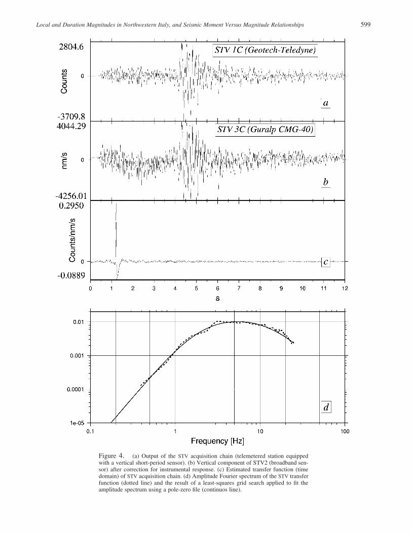
1C). Reliable ampli-tude-frequency response of each short-period instrumenta-tion system is not currently available. An empirical estimateof the transfer function is obtained comparing the waveformsof the same earthquake recorded by both short-period andbroadband sensors installed at the same site. This referencesite, indicated by a star in Figure 1, is equipped with both atelemetered short-period station (code STV) and a 3C broad-band digital station (code STV2). The input vertical groundmotion, which is assumed to be the same for both sensors,is evaluated correcting the vertical component of STV2 forits (known) instrument response. Then, the unknown transferfunction of the whole acquisition chain (field package andtransmission equipment) relevant to station STV is deter-mined by deconvolving the input ground motion from theoutput recordings. The spectral deconvolution is performedover the range 0.4 to 25 Hz. Figure 4 depicts an example of1C whole-chain transfer function retrieval: (a) the outputof the STV acquisition chain; (b) the vertical component ofSTV2 after correction for instrumental response; (c) the es-timated transfer function (time domain) of STV acquisitionchain; (d) its amplitude Fourier spectrum (dotted line) andthe result of a least-squares grid search applied to fit theamplitude spectrum using a pole-zero file (continuous line).This procedure is repeated for 10 earthquakes in the mag-nitude range 2 to 4, and the average transfer function is com-puted. This function is assumed to describe the system re-sponse of all the telemetered stations except for the gainvalue, which could differ from station to station. Amplitudenoise analysis (not reported in this article) is performed toensure that the gain value for each station is time indepen-dent from 1996 to 2003.

The synthetic maximum Wood-Anderson amplitudesderived from telemetered short-period network are used tocalibrate an amplitude magnitude scale for each 1C stationby using the following approach:

M � log(A/G) � n log(R/100) � k(R � 100) � S � 3(5)� log(A) � log(R/100) � k(R � 100) � S� � 3 ,

where M is the local magnitude value used to calibrate thescale, A is the maximum vertical synthetic Wood-Andersonamplitude, G is the unknown gain value, n and k are theattenuation parameters, R is the hypocentral distance, and Sis the station correction. We assume n � 1 and we introduce


Figure 3. (Left) Local magnitudes estimated in this study versus Spallarossa et al.(2002). (Right). Attenuation function log A � n log(R/100) � k(R � 100) for n �1, k � 0.0054 (this study, black line) and n � 1.144, k � 0.00476 (Spallarossa et al.,2002, dotted line).

S� � S � log(G), which is a station correction that accountsfor both magnitude correction and gain value. Given a setof earthquakes having known local magnitude M, computedaccording to the ML

3C scale, equation (5) is used to calibratek and S� for the short-period network constraining the cor-rection S� of station STV to zero. The calibration is per-formed considering 16,166 amplitudes from 2730 earth-quakes recorded at 12 stations in the distance range from 10to 310 km. The linear system is solved in a least-squaressense with the same method adopted for the calibration ofthe 3C scale. The obtained k is (0.0041 � 0.0001), and thestation corrections S� are shown in Table 3.

Duration Magnitude

We calibrated a magnitude scale based on signal dura-tion of the form (Real and Teng 1973; Herrmann, 1975):

M � c � c R � c log s (6)D 0 1 2

where s is the particular duration used and R is the hypo-central distance. In the present work, the duration is definedas the interval between the onset of the first arrival and thepoint at which the signal-to-noise ratio is definitely less than1.5. The signal-to-noise ratio is computed considering a pre-event window 2 sec wide, and s is estimated based on seis-mograms filtered in the frequency band 1–12 Hz. The cali-bration is performed by considering 10,842 recordings from2538 earthquakes recorded at 12 stations in the distancerange from 10 to 310 km. Table 3 lists the c0, c1, and c2

coefficients for all the stations. Small values for c1 are foundto be in agreement with a weak dependence of signal dura-tion on distance.

Validation

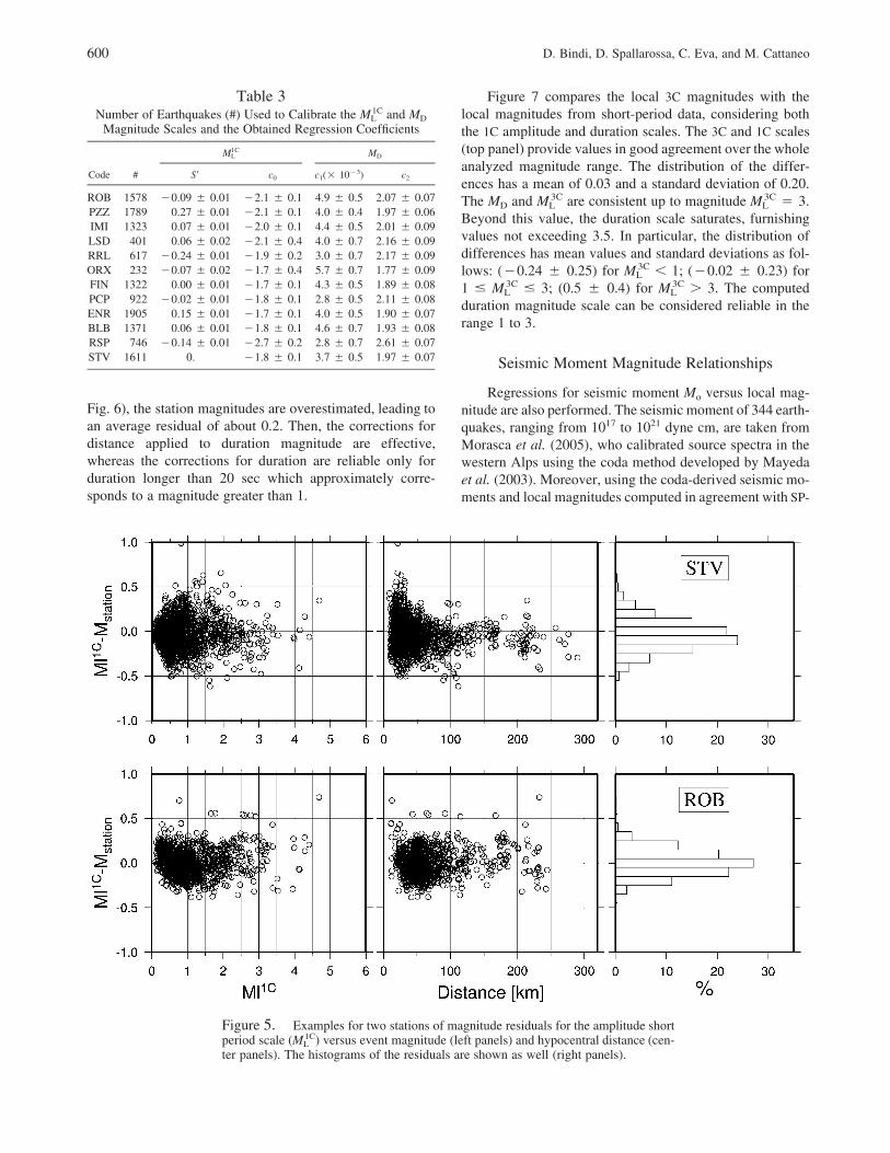
Earthquakes recorded from 1996 to 1998 are used tovalidate the obtained magnitude relationships. Figure 5shows the 1C magnitude residuals, that is, the difference be-tween the station magnitude and the arithmetic mean of thestation magnitudes for the same event (event magnitude)versus the hypocentral distance (center panels). The depen-dence on the event magnitude (left panels) and the histo-grams of the residuals (right panels) are shown as well. Theresults for the two selected stations in Figure 5 are represen-tative of the results obtained for all the other stations. Theresiduals do not show any significant trend with distance,suggesting that the applied correction in term of k properlyaccounted for the attenuation characteristics in the area. Theaverage residuals range from 0.001 (station BLB) to 0.04(STV and ROB stations) and, in general, the standard devi-ation is close to 0.2.

Figure 6 shows the duration magnitude residuals versusduration (left frames) and distance (center frames). The his-tograms of residuals are shown as well (right frames). Theaverage residual varies from 0.03 (STV) to 0.05 (BLB), andthe standard deviation is 0.2. The residuals are nearly inde-pendent of distance, whereas they increase with decreasingduration over the short-duration range. In particular, for du-ration less than 20 sec (log s � 1.3, vertical dotted lines in


Figure 4. (a) Output of the STV acquisition chain (telemetered station equippedwith a vertical short-period sensor). (b) Vertical component of STV2 (broadband sen-sor) after correction for instrumental response. (c) Estimated transfer function (timedomain) of STV acquisition chain. (d) Amplitude Fourier spectrum of the STV transferfunction (dotted line) and the result of a least-squares grid search applied to fit theamplitude spectrum using a pole-zero file (continuos line).


Table 3Number of Earthquakes (#) Used to Calibrate the ML

1C and MD

Magnitude Scales and the Obtained Regression Coefficients

ML1C MD

Code # S� c0 c1(� 10�3) c2

ROB 1578 �0.09 � 0.01 �2.1 � 0.1 4.9 � 0.5 2.07 � 0.07PZZ 1789 0.27 � 0.01 �2.1 � 0.1 4.0 � 0.4 1.97 � 0.06IMI 1323 0.07 � 0.01 �2.0 � 0.1 4.4 � 0.5 2.01 � 0.09LSD 401 0.06 � 0.02 �2.1 � 0.4 4.0 � 0.7 2.16 � 0.09RRL 617 �0.24 � 0.01 �1.9 � 0.2 3.0 � 0.7 2.17 � 0.09ORX 232 �0.07 � 0.02 �1.7 � 0.4 5.7 � 0.7 1.77 � 0.09FIN 1322 0.00 � 0.01 �1.7 � 0.1 4.3 � 0.5 1.89 � 0.08PCP 922 �0.02 � 0.01 �1.8 � 0.1 2.8 � 0.5 2.11 � 0.08ENR 1905 0.15 � 0.01 �1.7 � 0.1 4.0 � 0.5 1.90 � 0.07BLB 1371 0.06 � 0.01 �1.8 � 0.1 4.6 � 0.7 1.93 � 0.08RSP 746 �0.14 � 0.01 �2.7 � 0.2 2.8 � 0.7 2.61 � 0.07STV 1611 0. �1.8 � 0.1 3.7 � 0.5 1.97 � 0.07

Fig. 6), the station magnitudes are overestimated, leading toan average residual of about 0.2. Then, the corrections fordistance applied to duration magnitude are effective,whereas the corrections for duration are reliable only forduration longer than 20 sec which approximately corre-sponds to a magnitude greater than 1.

Figure 7 compares the local 3C magnitudes with thelocal magnitudes from short-period data, considering boththe 1C amplitude and duration scales. The 3C and 1C scales(top panel) provide values in good agreement over the wholeanalyzed magnitude range. The distribution of the differ-ences has a mean of 0.03 and a standard deviation of 0.20.The MD and ML

3C are consistent up to magnitude ML3C � 3.

Beyond this value, the duration scale saturates, furnishingvalues not exceeding 3.5. In particular, the distribution ofdifferences has mean values and standard deviations as fol-lows: (�0.24 � 0.25) for ML

3C � 1; (�0.02 � 0.23) for1 � ML

3C � 3; (0.5 � 0.4) for ML3C � 3. The computed

duration magnitude scale can be considered reliable in therange 1 to 3.

Seismic Moment Magnitude Relationships

Regressions for seismic moment Mo versus local mag-nitude are also performed. The seismic moment of 344 earth-quakes, ranging from 1017 to 1021 dyne cm, are taken fromMorasca et al. (2005), who calibrated source spectra in thewestern Alps using the coda method developed by Mayedaet al. (2003). Moreover, using the coda-derived seismic mo-ments and local magnitudes computed in agreement with SP-

Figure 5. Examples for two stations of magnitude residuals for the amplitude shortperiod scale (ML

1C) versus event magnitude (left panels) and hypocentral distance (cen-ter panels). The histograms of the residuals are shown as well (right panels).


02, they also calibrated an equivalent local magnitude scalethat provides very stable single-station magnitude values.Most of the earthquakes we considered have seismic mo-ments less than 1020 dyne cm, and only six events havehigher seismic moments. Because all the considered seismicmoments are relevant to earthquakes occurring in the west-ern Alps, the derived relationships can be considered reliableonly inside this area.

We carry out moment versus magnitude regression anal-ysis considering both the ML

3C and the ML1C scales. In general,

when computed over a broad magnitude range, the relationlog M0 versus magnitude shows a continuous positive cur-vature (Bakun, 1984; Hanks and Boore, 1984), that is, thelinear model log M0 � cML � d requires c values thatincrease with ML. It follows that a quadratic term is neededto fit data ranging over a wide range with a single scalingrelation (Hanks and Boore, 1984; Ben-Zion and Zhu, 2002).The need of a quadratic term was explained by Hanks andBoore (1984) as resulting from the complex interaction, inthe frequency domain, between the Wood-Anderson re-sponse spectrum and an x-square source model with con-

stant stress drop, whereas Ben-Zion and Zhu (2002) sug-gested an alternative possible explanation based on theassumption that “the occurrence of increasingly larger eventsis associated with increasingly smoother stress field” (Ben-Zion and Zhu, 2002, p. F2).

Figure 8 shows log Mo against both ML1C and ML

3C. Onlythe results obtained considering the linear model are shown,because the solutions for both the linear and quadratic re-lations produce the same root mean square of residuals (e.g.,0.14 in ML

3C). This result was expected because the bulk ofanalyzed magnitudes is in the range of 0 to 2.5, and onlynine earthquakes have a magnitude larger than 2.5. The bestleast-squares fits are:

1Clog M � (0.95 � 0.01) M � (17.36 � 0.01)0 L3Clog M � (0.92 � 0.01) M � (17.38 � 0.08)0 L

For a magnitude less than 2.5, these relations are similar tothe result found in the northeastern Alps (Granet and Hoang

Figure 6. Examples for two stations of magnitude residuals for the duration scale(MD) versus logarithm of duration (left panels) and distance (middle panels). The du-ration is measured in seconds. The histograms of the residuals (right panels) are shownas well. In the left panels, the vertical dotted lines at log s � 1.3 indicate the assumedlower bound of validity of the magnitude duration scale.


Trong, 1980), whereas a better agreement with the resultsfound for southwestern Germany (Sherbaum and Stoll,1983) is observed at higher magnitudes (Fig. 8).

Conclusions

We developed magnitude calibration analysis in north-western Italy by using three-component broad- or semi-broadband stations and recordings from vertical short-periodseismometers. The local magnitude scale computed using

10,057 synthetic Wood-Anderson maximum amplitudes(2822 earthquakes) from the horizontal components of thebroad- or semibroadband sensors is:

3CM � log A � log(R/100)L

� 0.0054(R � 100) � 3 � S

for magnitudes in the range 0 � ML � 5 and hypocentraldistance R from 10 to 310 km. The station corrections S vary

Figure 7. (top) Comparison between ML3C and

ML1C. (bottom) Comparison between ML

3C and MD.The histograms of differences are shown inside eachpanel.

Figure 8. Seismic moment versus ML1C (top) and

ML3C (bottom). The gray lines are the best least-

squares fits and the dashed and dotted lines are therelationships valid for the northeastern Alps (Granetand Hoang Trong, 1980) and southwestern Germany(Sherbaum and Stoll, 1983), respectively.


from �0.13 to 0.57, assuming that S for the reference stationSTV2 is zero. The magnitudes ML

3C predicted by this equa-tion are used to calibrate scales based on either syntheticWood-Anderson maximum amplitude (ML

1C scale) or totalsignal duration (MD scale), starting from vertical short-period recordings. The computed ML

1C scale is

1CM � log A � log(R/100)L

� 0.0041(R � 100) � 3 � S�

which we obtained by using the same reference site adoptedfor deriving ML

3C.The reliability of these scales has been assessed by com-

paring the predicted magnitudes with ML3C, using 827 earth-

quakes not included in the regression analysis. Although theML

1C and the ML3C scales showed good agreement over the

range 0 to 5, the strategy adopted for evaluating the signalduration s, that is, the selected corner frequencies of thebandpass filter and the threshold value assumed to determines, lead to reliable MD only over the range 1 to 3. Becausealternative strategies that allowed us to enlarge the rangetoward higher magnitudes always corresponded to an in-crease of the lower bound of the reliable magnitude range,in the present work, we adopted the settings that providedreliable duration magnitudes over the most sampled rangeof our dataset (1 � MD � 3).

Considering the local magnitudes for the three compo-nent stations (ML

3C) and those for the vertical, short-periodstations (ML

1C), the following seismic moment versus mag-nitude relationships have been derived for the western Alps:

3Clog M � (0.92 � 0.01) M � (17.38 � 0.08)0 L1Clog M � (0.95 � 0.01) M � (17.36 � 0.01)0 L

The reliability of the obtained amplitude scale for the short-period network allows us to compile a seismic catalog in-cluding local magnitudes and seismic moments over thewhole working period of the 1C network (from 1985 up to-day).

Acknowledgments

We thank P. Augliera for fruitful discussions and the staff of the RSNInetwork for their technical support. Suggestions from two anonymous re-viewers strongly improved this article. The figures were drawn using theGMT software (Wessel and Smith, 1990). This research has been supportedin part by Project GNDT2000-2002 coordinated by A. Amato and fundedby Italian Civil Protection.

References

Bakun, W. H. (1984). Seismic moments, local magnitudes, and coda-duration magnitudes for earthquakes in central California, Bull. Seism.Soc. Am. 74, 439–458.

Bakun, W. H., and W. B. Joyner (1984). The Ml scale in central California,Bull. Seism. Soc. Am. 74, 1827–1843.

Baumbach, M., D. Bindi, H. Grosser, C. Milkereit, S. Parolai, R. J. Wang,S. Karakisa, S. Zunbul, and J. Zschau (2003) Ml scale in northwesternTurkey from 1999 Izmit aftershocks, Bull. Seism. Soc. Am. 93, 2289–2295.

Ben-Zion, Y., and L. Zhu (2002). Potency-magnitude scaling relations forsouthern California earthquakes with 1.0 � Ml � 7.0, Geophys. J.Int. 148, F1–F5.

Bormann, P. (2002). Magnitude of seismic events, in IASPEI, New Manualof Seismological Observatory Practice, P. Bormann (Editor), Vol. 1,GeoForschungsZentrum, Potsdam, 16–50.

Capponi, G., M. Cattaneo, and F. Merlanti (1985). The Ligurian earthquakeof February 23, 1887, in Atlas of Isoseismal Maps of Italian Earth-quakes, D. Postpischl (Editor), Vol. 114, 2A, CNR-PFG, Rome, 100–103.

Cattaneo, M., and P. Augliera (1990). The automatic phase picking andevent location system at the IGG network, Cah. Cent. Eur. Geodin.Seism. 1, 65–74.

Cattaneo, M., P. Augliera, S. Parolai, and D. Spallarossa (1999). Anoma-lously deep earthquakes in northwestern Italy, J. Seism. 3, 421–435.

Cattaneo, M., P. Federici, and F. Merlanti (1981). L’uso della durata dellaregistrazione come misura della magnitudo per terremoti vicini,C.N.R, Progetto Finalizzato Geodinamica: Seminario sulla magni-tudo, Pubblicazione no. 481, (in Italian).

Efron, B. (1979). Bootstrap methods, another look at jacknife, Ann. Stat.7, 1–26.

Eva, E., S. Solarino, and D. Spallarossa (2001). Seismicity and crustal struc-ture beneath the western Ligurian derived from local earthquake to-mography, Tectonophysics 339, 495–510.

Ferrari, G., V. Petrini, E. Patacca, and P. Scandone (1985). The Garfaguanaearthquake of September 7, 1920, in Atlas of Isoseismal Maps ofItalian Earthquakes, D. Postpischl (Editor), Vol. 114, 2A, CNR-PFG,Rome, 130–135.

Granet, M., and P. Hoang Trong (1980). Some medium properties at Friuli(Italy) from amplitude spectrum Tectonophysics 137, 167–182.

Hanks, T. C., and D. M. Boore (1984). Moment-magnitude relations intheory and practice, J. Geophys. Res. 89, 6229–6235.

Herrmann, R. B. (1975). The use of duration as a measure of seismic mo-ment and magnitude, Bull. Seism. Soc. Am. 65, 899–913.

Kanamori, H. (1983). Magnitude scale and quantification of earthquakes,Tectonophysics 93, 185–199.

Langston, C. A., R. Brazer, A. A. Nyblade, and T. J. Owens (1998). Localmagnitude scale and seismicity rate for Tanzania, east Africa, Bull.Seism. Soc. Am. 88, 712–721.

Lee, W. H. K., and J. C. Lahr (1975). HYPO71 (revised): a computerprogram for determining hypocenter, magnitude, and first motion pat-tern of local earthquakes. U.S. Geol. Surv. Open-File Rept. 75-311,100 pp.

Mayeda, K., A. Hofstetter, J. L. O’Boyle, and W. R. Walter (2003). Stableand transportable regional magnitudes based on coda-derived mo-ment-rate spectra, Bull. Seism. Soc. Am. 93, 224–239.

Morasca, P., K. Mayeda, L. Malagnini, and W. R. Walter (2005). CodaDerived Source Spectra, Moment Magnitudes, and Energy-MomentScaling in the Western Alps, Geophys. J. Int. 160, 263–275.

Paige, C. C., and M. A. Saunders (1982). LSQR: an algorithm for sparselinear equations and sparse least squares, ACM Trans. Math. Soft. 8,43–71.

Real, C. R., and T. L. Teng (1973). Local Richter magnitude and total signalduration in Southern California, Bull. Seism. Soc. Am. 63, 1809.

Richter, C. F. (1935). An instrumental earthquake magnitude scale, Bull.Seism. Soc. Am. 25, 1–31.

Richter, C. F. (1958). Elementary Seismology, W. H. Freeman and Co., SanFrancisco, 578 pp.

Scherbaum, F., and D. Stoll (1983). Source parameters and scaling laws ofthe 1978 Swabian Jura (southwest Germany) aftershocks, Bull. Seism.Soc. Am. 137, 1321–1343.


Solarino, S., G. Ferretti, and C. Eva (2002). Seismicity of the Garfagnana-Lunigiana (Tuscany, Italy) as recorded by a network of semi-broadband instruments, J. Seism. 6, 141–152

Solarino, S., E. Kissling, S. Sellami, F. Thouvenot, K. P. Bonjer, M. Granet,and G. Smeriglio (1997). Local earthquake catalog 1980 to 1995 ofAlpine-Northern Apennine region for crustal seismic tomography,Ann. Geofis. 40, 161–174.

Spallarossa, D., D. Bindi, P. Augliera, and M. Cattaneo (2002). An MLScale in Northwestern Italy, Bull. Seism. Soc. Am. 90, 1062–1081.

Spallarossa, D., G. Ferretti, P. Augliera, D. Bindi, and M. Cattaneo (2001).Reliability of earthquake location procedure in heterogeneous areas:synthetic tests in the South Western Alps, Italy, Phys. Earth Planet.Int. 123, 247–266.

Uhrhammer, R. A., and E. R. Collins (1990). Synthesis of Wood-Andersonseismograms from broadband digital records, Bull. Seism. Soc. Am.80, 702–716.

Uhrhammer, R. A., S. J. Loper, and B. Romanowiez (1996). Determinationof local magnitude using BDSN broadband records, Bull. Seism. Soc.Am. 86, 1314–1330.

Wessel, P., and W. H. F. Smith (2000). The Generic Mapping Tools (GMT),version 3.3.6, gmt.soest.hawaii.edu/gmt.html (last accessed October2000).

Istituto Nazionale di Geofisica e Vulcanologiavia Bassini 1520133 Milan, Italy

(D.B.)

DipTeRis, University of GenoaViale Benedetto XV, 516132, Genoa, Italy

(D.S., C.E.)

Istituto Nazionale di Geofisica e Vulcanologiavia di Vigna Murata 60500143, Rome, Italy

(M.C.)

Manuscript received 24 May 2004.

Local and Duration Magnitudes in Northwestern Italy, … 44N29.48 10E0395 0.87 Lennartz LE3D-5s (3C)...

Documents

Transcript of Local and Duration Magnitudes in Northwestern Italy, … 44N29.48 10E0395 0.87 Lennartz LE3D-5s (3C)...