Local analyses of Planck maps with Minkowski Functionals · Local analyses of Planck maps with...

Mon. Not. R. Astron. Soc. 000, 1–11 (2013) Printed 14 June 2016 (MN LATEX style file v2.2)

Local analyses of Planck maps with Minkowski Functionals

C. P. Novaes1? A. Bernui1† G. A. Marques1‡ and I. S. Ferreira2§1Observatorio Nacional, Rua General Jose Cristino 77, Sao Cristovao, 20921-400 Rio de Janeiro, RJ, Brazil2Instituto de Fısica, Universidade de Brasılia, Campus Universitario Darcy Ribeiro, Asa Norte, 70919-970, Brasılia, DF, Brazil

Accepted xxxx. Received xxxx; in original form xxxx

ABSTRACTMinkowski Functionals (MF) are excellent tools to investigate the statistical propertiesof the cosmic background radiation (CMB) maps. Between their notorious advantagesis the possibility to use them efficiently in patches of the CMB sphere, which allowstudies in masked skies, inclusive analyses of small sky regions. Then, possible devia-tions from Gaussianity are investigated by comparison with MF obtained from a set ofGaussian isotropic simulated CMB maps to which are applied the same cut-sky masks.These analyses are sensitive enough to detect contaminations of small intensity likeprimary and secondary CMB anisotropies. Our methodology uses the MF, widely em-ployed to study non-Gaussianities in CMB data, and asserts Gaussian deviations onlywhen all of them points out an exceptional χ2 value, at more than 2.2σ confidencelevel, in a given sky patch. Following this rigorous procedure, we find 13 regions in theforeground-cleaned Planck maps that evince such high levels of non-Gaussian devia-tions. According to our results, these non-Gaussian contributions show signatures thatcan be associated to the presence of hot or cold spots in such regions. Moreover, someof these non-Gaussian deviations signals suggest the presence of foreground residualsin those regions located near the galactic plane. Additionally, we confirm that most ofthe regions revealed in our analyses, but not all, have been recently reported in stud-ies done by the Planck collaboration. Furthermore, we also investigate whether thesenon-Gaussian deviations can be possibly sourced by systematics, like inhomogeneousnoise and beam effect in the released Planck data, or perhaps due to residual galacticforegrounds.

Key words: cosmology: cosmic microwave background – cosmology: observations –Gaussian distributions

1 INTRODUCTION

The cosmic microwave background (CMB) temperature fluc-tuations encode in their statistical properties unique probesof the physical processes of the early universe. Convinc-ing detections of primordial non-Gaussian deviations in theCMB data, with characteristic type, amplitude, and scaledependence, provide invaluable information of the primevalevolution of density fluctuations (Bartolo et al. 2004; Smidtet al. 2010). However, non-Gaussian signals could also besourced from late processes as, e.g., gravitational lens-ing, Sunyaev-Zel’dovich effect, contaminant radiations fromgalactic foregrounds and from residual point sources, etc.,and, moreover, signatures from these non-Gaussian con-tributions could be confused with primordial ones, which

? e-mail: [email protected]† e-mail: [email protected]‡ e-mail: [email protected]§ e-mail: [email protected]

makes necessary detailed analyses of the CMB data (Han-son et al. 2009; Lacasa 2014; Serra & Cooray 2008; PlanckCollaboration 2015c,e).

After accurate analyses performed on the recentlyreleased high resolution foreground-cleaned CMB maps,the Planck collaboration found primordial non-Gaussianity(NG) of small intensity that supports the simplest infla-tionary scenario of a single-field model (Planck Collabora-tion 2015e). In addition, complementary analyses providedstrong constraints for the presence of secondary NGs in thesemaps, in particular for foregrounds residuals and contami-nations from systematics (Axelsson et al. 2015; Planck Col-laboration 2015e). Considering that no single statistical es-timator is able to identify all possible forms of NG, it isworth to examine the Planck CMB data (Planck Collabo-ration 2015a) not only for confirmation of the reported re-sults, but more interestingly, to perform independent anal-yses with diverse statistical tools applied with different in-spection methodologies. For this, a variety of non-Gaussianestimators and strategies has been introduced in the lit-

c© 2013 RAS

arX

iv:1

606.

0407

5v1

[as

tro-

ph.C

O]

13

Jun

2016

2 C. P. Novaes, A. Bernui, G. A. Marques, and I. S. Ferreira

erature with the scope to detect primary and secondarynon-Gaussian contributions left in CMB data (see, for in-stance, Babich (2005); Bartolo et al. (2010, 2012); Noviello(2009); Pietrobon et al. (2009); Vielva et al. (2004); Vielva& Sanz (2009); Matsubara (2010); Cabella et al. (2010);Nørgaard-Nielsen (2010); Casaponsa et al. (2011a,b); Rossiet al. (2011); Smith et al. (2011); Donzelli et al. (2012);Ducout et al. (2012); Fergusson et al. (2012); Pratten &Munshi (2012); Bernui & Reboucas (2012); Bernui et al.(2014); Bernui & Reboucas (2015); Novaes et al. (2014)).The search for NGs in the CMB maps includes galactic andextra-galactic sources, and also possible contributions fromsystematic effects, like inhomogeneous noise, cut-sky masks,Doppler and aberration effects, etc. (Saha 2011; Vielva 2010;Novaes et al. 2015; Quartin & Notari 2015).

Here we use the well-known Minkowski Functionals(MF) (Minkowski 1903; Novikov et al. 1999; Komatsu etal. 2003; Hikage & Matsubara 2012; Munshi et al. 2012,2013) to perform a detailed local analysis of the foreground-cleaned Planck CMB maps, searching for Gaussian devia-tions in 192 regions (i.e., pixels with size ' 14.7) in whichthe CMB sphere is divided. Our main motivations for theselocal non-Gaussian scrutiny are:(i) to confirm previous results, that is, finding anomalousnon-Gaussian regions in the CMB temperature field, alreadyreported by other teams, including the Planck collaboration;(ii) to identify, or at least throw some light on, the sourcesof the NG revealed in these anomalous regions by compar-ing their signatures imprinted in the MF with some knownnon-Gaussian phenomena, for instance, the signature leftby foreground residuals or systematics (like inhomogeneousnoise);(iii) to perform complementary analyses that let us to findanomalous unreported regions.In our scrutiny we found 13 regions where Gaussian devia-tions, as measured by the MF, show anomalous χ2 values,at more than 2.2σ confidence level, when compared withGaussian CMB maps.

In this way, in section 2 we start presenting the PlanckCMB maps used in the analysis. In section 3 we introducethe tools that we use to reveal NGs, that is, the MF, as wellas the basic concepts of how to use them. Sections 4 and 5compiles the methodology applied to the Planck CMB mapsand show our results, while we present our conclusions andfinal remarks in section 6.

2 THE PLANCK DATA PRODUCTS

In 2015, the Planck Collaboration released the second set ofproducts derived from the Planck dataset1. Between themare the four CMB foreground-cleaned maps, namely (PlanckCollaboration 2015b): Spectral Matching Independent Com-ponent Analysis (SMICA), Needlet Internal Linear Combi-nation (NILC), Spectral Estimation Via Expectation Max-imization (SEVEM), and the Bayesian parametric methodCommander, names originated from the separation method

1 Based on observations obtained with Planck(http://www.esa.int/Planck), an ESA science mission withinstruments and contributions directly funded by ESA Member

States, NASA, and Canada.

used to produce them. These high resolution maps haveNside = 2048 and effective beam fwhm = 5′.

The performance of the foreground-cleaning algorithmshas been carefully investigated by the Planck collaborationwith numerous sets of simulated maps (Planck Collabora-tion 2015b). In particular, each component separation algo-rithm processed differently the multi-contaminated sky re-gions obtaining, as a consequence, different final foreground-cleaned regions for each procedure. These regions are de-fined outside the so-called Component Separation Confi-dence masks, released jointly to the associated CMB map,corresponding to fsky = 0.85, 0.96, 0.84, 0.82, for the SMICA,NILC, SEVEM, and Commander maps, respectively. The Planckteam also released the UT78 mask, which is the union of theabove mentioned masks, a more restrictive one, since it hasfsky = 0.776, and adopted as the preferred mask for analyz-ing the temperature maps (Planck Collaboration 2015b).

Our analyses were performed upon the products of thePlanck’s second data release. Furthermore, the UT78 maskwas used in all the investigated cases.

3 THE MINKOWSKI FUNCTIONALS

The MF present many advantages as compared with otherstatistical estimators. One of them is their versatility in de-tecting diverse types of NG without a previous knowledge oftheir features, such as their angular dependence or intensity,and also because they can be efficiently applied in maskedskies or still in small regions of the CMB sphere.

The morphological properties of data in a d-dimensionalspace can be described using d + 1 MF (Minkowski 1903).For a 2-dimensional CMB temperature field defined on thesphere S2, ∆T = ∆T (θ, φ), with zero mean and variance σ2,this tool provides a test of non-Gaussian features by assess-ing the properties of connected regions in the map (Komatsuet al. 2003; Modest et al. 2013). Given a sky path P of thepixelized CMB sphere S2, an excursion set of amplitude νtis defined as the set of pixels in P where the temperaturefield exceeds the threshold νt, that is, the set of pixels withcoordinates (θ, φ) ∈ P such that ∆T (θ, φ)/σ ≡ ν > νt. Eachexcursion set, or connected region, Σ, with ν > νt, and itsboundary, ∂Σ, can be defined as

Σ ≡ (θ, φ) ∈ P | ∆T (θ, φ) > νσ, (1)

∂Σ ≡ (θ, φ) ∈ P | ∆T (θ, φ) = νσ. (2)

In a 2-dimensional case, for a region Σ ⊂ S2 with amplitudeνt the partial MF calculated in Ri are: ai, the Area of theregion described by Σ, li, the Perimeter, or contour length,∂Σ of this region, and ni, the number of holes inside Σ. Theglobal MF are obtained calculating these quantities for allthe connected regions with height ν > νt. Then, the totalArea V0(ν), Perimeter V1(ν) and Genus V2(ν) are (Novikovet al. 1999; Komatsu et al. 2003; Naselsky et al. 2006; Ducoutet al. 2012)

V0(ν) =1

4π

∫Σ

dΩ =∑

ai , (3)

V1(ν) =1

4π

1

4

∫∂Σ

dl =∑

li , (4)

c© 2013 RAS, MNRAS 000, 1–11

Local analyses of Planck maps with Minkowski Functionals 3

V2(ν) =1

4π

1

2π

∫∂Σ

κ dl =∑

ni = Nhot −Ncold , (5)

where dΩ and dl are, respectively, the elements of solidangle and line. In the Genus definition, the quantity κ isthe geodesic curvature (for details see, e.g., Ducout et al.(2012)). This last MF can also be calculated as the differencebetween the number of regions with ν > νt (number of hotspots, Nhot) and regions with ν < νt (number of cold spots,Ncold).

The calculations of the MF used here were done usingthe algorithm developed by Ducout et al. (2012) and Gay etal. (2012).

4 METHODOLOGY FOR DATA ANALYSES

4.1 The local analysis

In our local analyses we use the resolution parameterNside = 512 for all CMB maps, data and synthetic ones,as well as for the UT78 mask, because higher resolutions donot improve significantly the information contained in theMF (Ducout et al. 2012). For this, we degrade the PlanckCMB maps and mask to this resolution using the HEALPix(Hierarchical Equal Area iso-Latitude Pixelization) pixeliza-tion grid (Gorski et al. 2005). All pixels of the degraded maskwith values different from 1 are set to 0. After that, we de-fine the sky patches where to carry out the local analysesand apply the MF in each region of the CMB sky individ-ually. These regions are defined by the pixels correspondingto a resolution of Nside = 4, that is, 192 pixels of equal area' 14.72. Each of these big pixels (hereafter called patches)contains 16,384 small pixels corresponding to the resolutionparameter Nside = 512. We use the UT78 mask to excludepossible galactic contaminations, consequently, the numberof valid pixels in each region, varies from one region to an-other.

Considering n different thresholds ν = ν1 , ν2 , ... νn, pre-viously defined dividing the range −νmax to νmax in n equalparts, we compute the three MF Vk, k = 0, 1, 2, for the p-thpatch of a CMB map, with p = 1, 2, ..., 192. Then, for thep-th patch and for each k we have the vector

vpk ≡ (Vk(ν1), Vk(ν2), ...Vk(νn))|for the p-th patch , (6)

for k = 0, 1, 2, that is, the Area, Perimeter, and Genus,respectively. The values chosen for such variables are(νmax, n) = (3.5, 26) (for details, see Ducout et al. (2012)).

Next section presents the results of calculating the MFfrom Planck data and comparing them to those extractedfrom a set of 5000 Monte Carlo (MC) CMB maps. Notethat such simulated data correspond to ideal CMB maps,that is, without any contribution from foreground residuals,instrumental noise or beam effect. Our purpose here is tobe able to carefully analyse the most significant differencesbetween the ideal and real cases. These random Gaussian re-alisations are seeded by the CMB angular power spectrum2,

2 There is a strong dependence of the amplitude of the MF with

the power spectrum shape (Hikage & Matsubara 2012). For this,we chose to use the CMB data angular power spectrum, available

jointly the second Planck data release, instead of the ΛCDM best-

fit. Thereby, the angular power spectra corresponding to synthetic

according to the last Planck results (Planck Collaboration2015d).

4.2 χ2 analyses of MC and Planck CMB maps

Studies of NG in CMB data were extensively done usingthese three MF. Regarding their performances in such anal-yses, it was reported that the Area is the less sensitive to re-veal NG (see, e.g., Ducout et al. (2012); Novaes et al. (2014,2015)). For this, we define a single 52-elements vector whichcombines only the Perimeter and Genus information into ajoint estimator

Vp ≡ (vp1 , v

p2)

= (V p1 (ν1), ..., V p

1 (ν26), V p2 (ν1), ..., V p

2 (ν26)) , (7)

calculated for each patch p = 1, 2, ..., 192. To avoid excessof indices, in what follows we do not explicitly write thesuper-index p when referring to the quantity V, but oneunderstands that it is being calculated for each patch p ofthe CMB map (Planck or simulated data).

Firstly, we use the joint estimator to calculate the meanvector 〈VMC〉 for the set of 5000 MC CMB maps. Then, wecalculate VPlanck for each Planck map to compare with themean vector 〈VMC〉, which contains the features expected inGaussian CMB maps. This is done performing a χ2 analysiswhich takes into account the correlations among the MFcalculating, for each patch, the quantity (Komatsu et al.2003; Ducout et al. 2012)

χ2 ≡52∑i=1

52∑j=1

[VPlancki − 〈VMC

i 〉]C−1i,j [VPlanck

j − 〈VMCj 〉], (8)

where the i and j indices run over all 52 combinations of thethresholds ν (26 for the Perimeter and 26 for the Genus),and C−1

i,j is the inverse of the full covariance matrix, Ci,j ,

which is calculated from the MC simulations as3

Ci,j ≡ 〈 (VMCi − 〈VMC

i 〉) (VMCj − 〈VMC

j 〉) 〉. (9)

The maps on Figure 1 represent, in a color scale, the χ2 val-ues resulting from the analysis of each sky region individ-ually. These maps, hereafter called χ2-maps, are producedfor each Planck CMB map.

The χ2-maps let us to evaluate two important issuesregarding the performance of our joint estimator: first, thesensitivity of each MF to the local features of the data mapsrelative to the synthetic ones, and second, the influence inour results of the number of valid pixels inside a patch (i.e.,those not excluded by the application of the UT78 mask).

(i) Sensitivity of the MF :The χ2-maps produced using the Equations (7) and (8) high-light some patches of the sky, whose χ2 value is significantlyhigher than the mean. It shows that Perimeter and Genus,

and Planck CMB data are more compatible, making unnecessaryto recalibrate the MF accordingly.3 The MF calculated at a sequence of thresholds ν, as well asfor diverse MF estimators, are correlated. In order to take suchproperty into account it is important to use a full covariancematrix, Ci,j , in the data analyses (Hikage et al. 2006; Ducout et

al. 2012).

c© 2013 RAS, MNRAS 000, 1–11


1

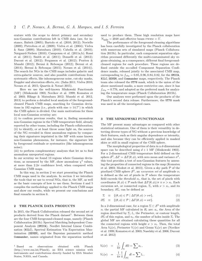
Figure 1. χ2-maps obtained from the joint estimator (Perimeter and Genus) calculated from the SMICA, SEVEM, NILC, and Commander

Planck maps (from left to right), in comparison to those obtained from a set of 5000 MC CMB maps. These χ2-maps show that thepatches with the higher χ2 values are the same for all the Planck maps.

combined into a joint estimator, are able to efficiently reveallocal Gaussian deviations in the Planck maps compared toMC Gaussian CMB data. For the sake of completeness, wehave also tested the behavior of the joint estimator in thecase that one includes the Area in its definition, Equation(7). In this case, the resulting χ2-maps (one for each Planckmap) reveal a rather featureless map with an almost uni-form distribution of values through the sky, evidencing anotable disagreement with the results presented in Figure 1(inclusive, the well-known anomalous Cold Spot (Vielva etal. 2004) passes undetected). These outcomes confirm thelower sensitivity of the Area relative to the others, and val-idates our previous choice of a Perimeter plus Genus jointestimator.

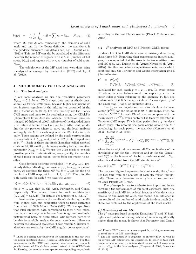
(ii) Influence of the percentage of valid pixels:Since all the current analysis are performed considering asky cut given by the UT78 mask, each patch of the sky iscomposed by a different number of valid pixels. In this sense,it is important to check if the percentage of valid pixels in-fluences our analysis. Figure 2 shows, for each Planck CMBmap, the dependence between the χ2 value and the percent-age of valid pixels in each patch. This comparison allowsus to observe that there is no evident relationship betweenthese two quantities. Nevertheless, from now on, we considerpatches with a minimum of 30% of valid pixels.

The results obtained in this section using the χ2-maps,suggest a more careful study of the set of patches that ex-hibit anomalously large χ2 values. For this we continue ouranalysis examining in detail the Perimeter and Genus curvescorresponding to these regions, in order to evidence its (pos-sible) peculiar signature that would lead to recognize itssource. Such analyses are presented through the next sec-tion.

5 ANALYSIS OF THE ANOMALOUSREGIONS

The aim of this section is the detailed analysis of the skypatches of the Planck CMB maps upon where the MFrevealed more significant differences relatively to the MCGaussian simulations. We constructed a total χ2-map byaveraging among the χ2-maps obtained for each PlanckCMB map (Figure 1), namely, the SMICA, SEVEM, NILC, andCommander

total χ2 = (χ2SMICA + χ2

SEVEM + χ2NILC + χ2

Commander)/4 . (10)

Figure 3 shows the total χ2-map, while the Figure 4 graphi-cally presents these total χ2 values as a function of the patch

1

Figure 2. Dependence of the χ2 values with the percentage of

valid pixels in the patches. The blue, yellow, red and green dotscorresponds, respectively, to the results from analysing the SMICA,

SEVEM, NILC, and Commander Planck maps (χ2-maps from left to

right in Figure 1). From now on, we consider patches with a min-imum of 30% of valid pixels.

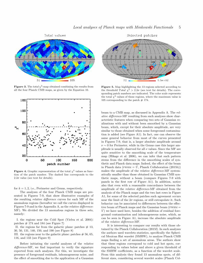
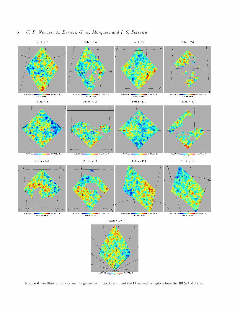
number. The horizontal dashed line represents the thresholdwe used as criterion for selecting the patches. This thresh-old value corresponds to the 2.2σ deviation (dashed line)calculated upon the values of the total χ2-map. Finally, weselected all the patches whose total χ2 values are higherthan 2.2σ level. As a result we find 13 sky patches showedin Figure 5, in a full-sky Mollweide projection, and in Fig-ure 6, as individual gnomview projections, which exhibitNG at a high confidence level (> 2.2σ). Once these regionsare selected, our MF analyses consider such 13 patches inthe four foreground-cleaned Planck maps. Hereafter we callthese patches anomalous regions.

Aiming to investigate particular features, like the am-plitude and signature, of the Gaussian deviations present inthe selected anomalous regions, we compare their MF vec-tors, vk (Equation 6), to the mean calculated from the MCGaussian CMB maps. For this we use the relative differencebetween them, defined as being the difference of both quan-tities normalized by the maximum value of the mean MFvector in analysis, that is,

relative difference-MFk ≡vPlanckk − 〈vk〉〈vk〉MAX

, (11)

c© 2013 RAS, MNRAS 000, 1–11


1

Figure 3. The total χ2-map obtained combining the results from

all the four Planck CMB maps, as given by the Equation 10.

1

Figure 4. Graphic representation of the total χ2 values as func-

tion of the patch number. The dashed line corresponds to the2.2σ value (see text for details).

for k = 1, 2, i.e., Perimeter and Genus, respectively.The analyses of the four Planck CMB maps are pre-

sented in Figures 7-9, that show illustrative examples ofthe resulting relative difference curves for each MF of theanomalous regions (hereafter we call the curves displayed inFigures 7-9 and in the Appendix A, as the relative difference-MF). We divided the 13 anomalous regions in three sets,namely:

I. the regions near the Cold Spot (Vielva et al. 2004):patches # 174 and 184 (see Figure 7)II. the regions far from the galactic plane: patches # 13,

30, 50, 131, 140, 150, and 190 (see Figure 8)III. the regions near to the galactic plane: patches # 56, 65,116, and 133 (see Figure 9)

Before initiating the careful analyses of the relativedifference-MF, we find important to verify the signatureexpected from such analyses. For this, we investigate thepresence of foreground residuals, inhomogeneous noise, andthe effect of smoothing due to the application of a Gaussian

1

Figure 5. Map highlighting the 13 regions selected according to

the threshold Total χ2 > 2.2σ (see text for details). The corre-

sponding patch numbers are indicated. The color scale representsthe total χ2 values of these regions, where the maximum value is

105 corresponding to the patch # 174.

beam to a CMB map, as discussed in Appendix A. The rel-ative difference-MF resulting from such analyses show char-acteristic features when comparing two sets of Gaussian re-alizations with and without been smoothed by a Gaussianbeam, which, except for their absolute amplitude, are verysimilar to those obtained when some foreground contamina-tion is added (see Figure A1). In fact, one can observe thesame general behavior from most of the curves presentedin Figures 7-9, that is, a larger absolute amplitude aroundν ∼ 0 for Perimeter, while in the Genus case this larger am-plitude is usually observed for all ν values. Since the MF arequite sensitive to the smoothing scale of the temperaturemap (Hikage et al. 2006), we can infer that such patternstems from the difference in the smoothing scales of syn-thetic and Planck data maps. Indeed, the effect of the beamin Planck data (fwhm = 5′, Planck Collaboration (2015b))makes the amplitude of the relative difference-MF system-atically smaller than those obtained in Gaussian CMB syn-thetic maps, without a beam (compare Figures 7-9 withpanels in the first row of Figure A1). In addition, noticealso that even with a reasonable concordance between theamplitude of the relative difference-MF obtained from theanalysis of the Planck maps and the two last rows in FigureA1, for some of the selected patches such agreement occursnear the limit of the 2σ regions, or still extrapolate it. Suchbehavior can be associated to differences between the effec-tive beam of Planck maps and the Gaussian beam (fwhm =5′) we have used here, besides the addition of residual fore-ground contamination and inhomogeneous noise, which, ascan be seen in Figure A1, increase the absolute amplitudeof the relative difference-MF.

It is interesting to compare our results with those ob-tained by the Planck Collaboration (2015f). In such analysesthe authors used wavelets statistics, specifically the Spheri-cal Mexican Hat wavelet (SMHW), to analyse Planck CMBmaps finding a set of anomalous areas. The authors showthat these regions correspond to cold and hot spots, cor-responding to values below and above a given threshold ofthe SMHW coefficients, as a function of the wavelet scale.From this analysis they found 13 anomalous spots, of dif-ferent sizes, considering several wavelet scales (Planck Col-

c© 2013 RAS, MNRAS 000, 1–11


1

Figure 6. For illustration we show the gnomview projections around the 13 anomalous regions from the SMICA CMB map .

c© 2013 RAS, MNRAS 000, 1–11


1

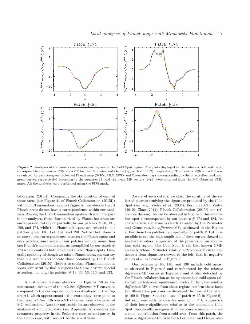
Figure 7. Analyses of the anomalous regions encompassing the Cold Spot region. The plots displayed in the columns, left and right,correspond to the relative difference-MF for the Perimeter and Genus (vk, with k = 1, 2), respectively. The relative difference-MF was

calculated for each foreground-cleaned Planck map (SMICA, NILC, SEVEM and Commander maps, corresponding to the blue, yellow, red, and

green curves, respectively) according to the equation 11, and the mean MF vectors (〈vk〉) were obtained from the MC Gaussian CMBmaps. All the analyses were performed using the UT78 mask.

laboration (2015f)). Comparing the sky position of each ofthese areas (see Figure 41 of Planck Collaboration (2015f))with our 13 anomalous regions (Figure 5), we observe that 4Planck areas do not have a correspondence within our anal-yses. Among the Planck anomalous spots with a counterpartin our analyses, those characterized by Planck hot areas areencompassed, totally or partially, by our patches # 50, 131,150, and 174, while the Planck cold spots are related to ourpatches # 65, 140, 174, 184, and 190. Notice that, there isno one-to-one correspondence between the Planck spots andours patches, since some of our patches include more thanone Planck’s anomalous spot, as exemplified by our patch #174 which contains both a hot and a cold Planck spots. Gen-erally speaking, although we miss 4 Planck areas, one can saythat our results corroborate those obtained by the PlanckCollaboration (2015f). Besides to confirm Planck anomalousspots, our scrutiny find 5 regions that also deserve specialattention, namely, the patches # 13, 30, 56, 116, and 133.

A distinctive feature observed in Figures 7-9 is thenon-smooth behavior of the relative difference-MF curves ascompared to the corresponding curves displayed in the Fig-ure A1, which appear smoothed because they correspond tothe mean relative difference-MF obtained from a large set ofMC realizations. Another noticeable feature observed in theanalyses of simulated data (see Appendix A) concerns thesymmetry property, in the Perimeter case, or anti-parity, inthe Genus case, with respect to the ν = 0 value.

Aware of such details, we start the scrutiny of the se-lected patches studying the signature produced by the ColdSpot (see, e.g., Vielva et al. (2004); Bernui (2009); Vielva(2010); Zhao (2014); Planck Collaboration (2015f) and ref-erences therein). As can be observed in Figure 6, this anoma-lous spot is encompassed by our patches # 174 and 184. Itscharacteristic signature is clearly revealed by the Perimeterand Genus relative-difference-MF, as showed in the Figure7. For these two patches, but specially for patch # 184, it ispossible to see the high amplitude of these curves skewed tonegative ν values, suggestive of the presence of an anoma-lous cold region. The Cold Spot is the best-known CMBanomaly whose Perimeter relative difference-MF curve evi-dence a clear signature skewed to the left, that is, negativevalues of ν, as noticed in Figure 7.

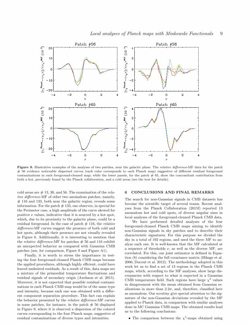
Our patches # 65, 140, and 190 include cold areas,as observed in Figure 6 and corroborated by the relativedifference-MF curves in Figures 8 and 9, also detected bythe Planck collaboration as being anomalous cold spots (al-though with diverse significance levels). In fact, the relativedifference-MF curves from these regions confirm these facts(for illustrative purposes we displayed the case of the patch# 190 in Figure 8 and the case of patch # 65 in Figure 9),but each one with its own features for ν < 0, suggestiveof their lower significance relative to the anomalous ColdSpot. Specifically, in region # 65 we observe around ν = −2a small contribution from a cold area. From this patch, therelative difference-MF, from both Perimeter and Genus, also

c© 2013 RAS, MNRAS 000, 1–11


1

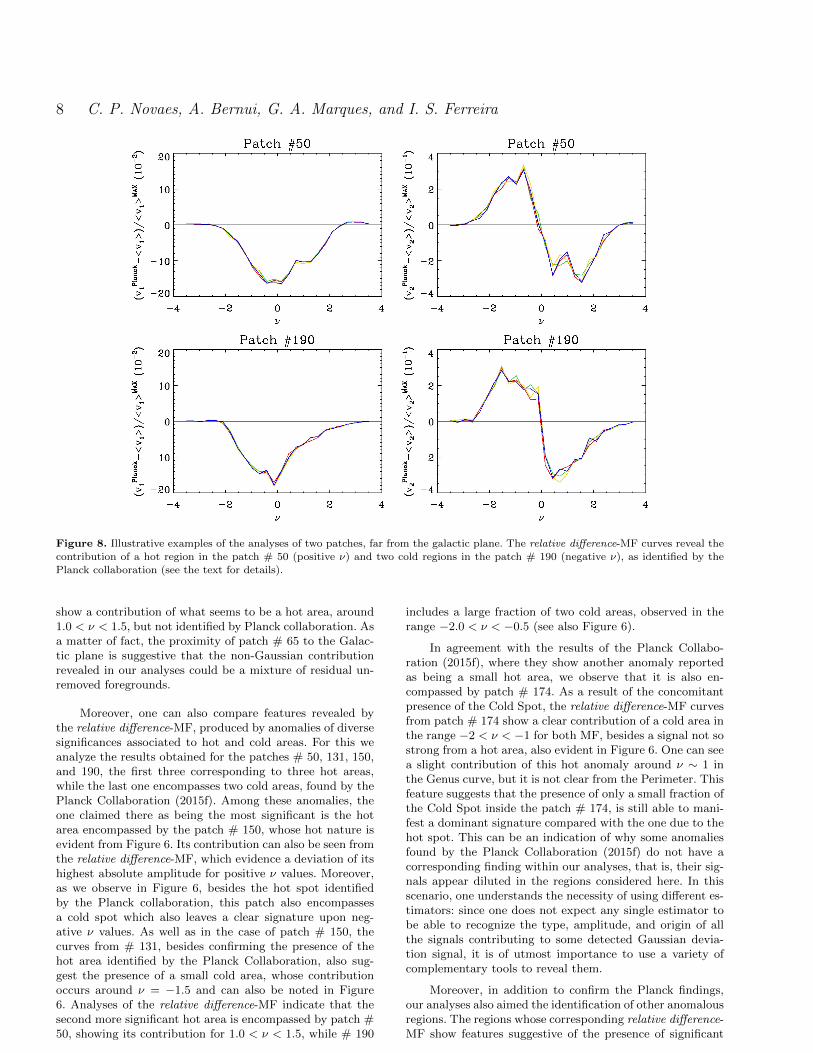
Figure 8. Illustrative examples of the analyses of two patches, far from the galactic plane. The relative difference-MF curves reveal thecontribution of a hot region in the patch # 50 (positive ν) and two cold regions in the patch # 190 (negative ν), as identified by the

Planck collaboration (see the text for details).

show a contribution of what seems to be a hot area, around1.0 < ν < 1.5, but not identified by Planck collaboration. Asa matter of fact, the proximity of patch # 65 to the Galac-tic plane is suggestive that the non-Gaussian contributionrevealed in our analyses could be a mixture of residual un-removed foregrounds.

Moreover, one can also compare features revealed bythe relative difference-MF, produced by anomalies of diversesignificances associated to hot and cold areas. For this weanalyze the results obtained for the patches # 50, 131, 150,and 190, the first three corresponding to three hot areas,while the last one encompasses two cold areas, found by thePlanck Collaboration (2015f). Among these anomalies, theone claimed there as being the most significant is the hotarea encompassed by the patch # 150, whose hot nature isevident from Figure 6. Its contribution can also be seen fromthe relative difference-MF, which evidence a deviation of itshighest absolute amplitude for positive ν values. Moreover,as we observe in Figure 6, besides the hot spot identifiedby the Planck collaboration, this patch also encompassesa cold spot which also leaves a clear signature upon neg-ative ν values. As well as in the case of patch # 150, thecurves from # 131, besides confirming the presence of thehot area identified by the Planck Collaboration, also sug-gest the presence of a small cold area, whose contributionoccurs around ν = −1.5 and can also be noted in Figure6. Analyses of the relative difference-MF indicate that thesecond more significant hot area is encompassed by patch #50, showing its contribution for 1.0 < ν < 1.5, while # 190

includes a large fraction of two cold areas, observed in therange −2.0 < ν < −0.5 (see also Figure 6).

In agreement with the results of the Planck Collabo-ration (2015f), where they show another anomaly reportedas being a small hot area, we observe that it is also en-compassed by patch # 174. As a result of the concomitantpresence of the Cold Spot, the relative difference-MF curvesfrom patch # 174 show a clear contribution of a cold area inthe range −2 < ν < −1 for both MF, besides a signal not sostrong from a hot area, also evident in Figure 6. One can seea slight contribution of this hot anomaly around ν ∼ 1 inthe Genus curve, but it is not clear from the Perimeter. Thisfeature suggests that the presence of only a small fraction ofthe Cold Spot inside the patch # 174, is still able to mani-fest a dominant signature compared with the one due to thehot spot. This can be an indication of why some anomaliesfound by the Planck Collaboration (2015f) do not have acorresponding finding within our analyses, that is, their sig-nals appear diluted in the regions considered here. In thisscenario, one understands the necessity of using different es-timators: since one does not expect any single estimator tobe able to recognize the type, amplitude, and origin of allthe signals contributing to some detected Gaussian devia-tion signal, it is of utmost importance to use a variety ofcomplementary tools to reveal them.

Moreover, in addition to confirm the Planck findings,our analyses also aimed the identification of other anomalousregions. The regions whose corresponding relative difference-MF show features suggestive of the presence of significant

c© 2013 RAS, MNRAS 000, 1–11


1

Figure 9. Illustrative examples of the analyses of two patches, near the galactic plane. The relative difference-MF data for the patch# 56 evidence noticeable dispersed curves (each color corresponds to each Planck map) suggestive of different residual foreground

contaminations in each foreground-cleaned map; while the lower panels, for the patch # 65, show the concomitant contribution from

both a hot, previously found by the Planck collaboration, and a cold areas (see the text for details).

cold areas are # 13, 30, and 56. The examination of the rela-tive difference-MF of other two anomalous patches, namely,# 116 and 133, both near the galactic region, reveals someinformation. For the patch # 133, one observes, in special forthe Perimeter case, a high amplitude of the curve skewed forpositive ν values, indicative that it is sourced by a hot spot,which, due to its proximity to the galactic plane, could be aresidual foreground. In the case of patch # 116, the relativedifference-MF curves suggest the presence of both cold andhot spots, although their presence are not visually revealedin Figure 6. Additionally, it is interesting to mention thatthe relative difference-MF for patches # 56 and 116 exhibitan unexpected behavior as compared with Gaussian CMBpatches (see, for comparison, Figure 9 and Figure A1).

Finally, it is worth to stress the importance in test-ing the four foreground-cleaned Planck CMB maps becausethe applied procedures, although highly efficient, could haveleaved undesired residuals. As a result of this, data maps area mixture of the primordial temperature fluctuations andresidual signals of secondary origin (Axelsson et al. 2015).Moreover, it is not expected that possible residual contami-nations in each Planck CMB map would be of the same typeand intensity, because each one was obtained with a differ-ent component separation procedure. This fact can explainthe behavior presented by the relative difference-MF curvesin some patches, for instance, in the patch # 56 displayedin Figure 9, where it is observed a dispersion of the coloredcurves corresponding to the four Planck maps, suggestive ofresidual contaminations of diverse types and intensities.

6 CONCLUSIONS AND FINAL REMARKS

The search for non-Gaussian signals in CMB datasets hasbecome the scientific target of several teams. Recent anal-yses from the Planck Collaboration (2015f) reported 13anomalous hot and cold spots, of diverse angular sizes inlocal analyses of the foreground-cleaned Planck CMB data.

We have performed detailed analyses of the fourforeground-cleaned Planck CMB maps aiming to identifynon-Gaussian signals in sky patches and to describe theircharacteristic signatures. For this purpose we divided thesky in a total of 192 regions, and used the three MF to an-alyze each one. It is well-known that the MF calculated ata sequence of thresholds ν, as well as the diverse MF, arecorrelated. For this, our joint estimator is defined in Equa-tion (8) considering the full covariance matrix (Hikage et al.2006; Ducout et al. 2012). The methodology adopted in thiswork let us to find a set of 13 regions in the Planck CMBmaps, which, according to the MF analyses, show large dis-crepancies with respect to what is expected in a GaussianCMB temperature field. Such regions have large χ2 valuesin disagreement with the mean obtained from Gaussian re-alizations in more than 2.2σ, and, therefore, classified hereas anomalous. Our scrutiny give special attention to the sig-nature of the non-Gaussian deviations revealed by the MFapplied to Planck data, in comparison with similar analysesdone in MC Gaussian CMB maps. The obtained results leadus to the following conclusions:

• The comparison between the χ2-maps obtained using

c© 2013 RAS, MNRAS 000, 1–11


the Area and those combining the other two MF to analysethe four Planck CMB maps (Figure 1) confirms the lowersensitivity of this MF relatively to the other two (noticed be-fore by Ducout et al. (2012) and Novaes et al. (2014, 2015)).

• The absence of a definite dependence among the χ2

values and the percentage of valid pixels, showed in Figure 2,evidence a weak dependence of the patch effective area inour analyses.

• The different χ2 values obtained in the Planck CMBmaps could be an indication of the presence of residual con-taminations in these foreground-cleaned CMB maps. How-ever, we observe that both χ2-maps, calculated for the fourPlanck maps, as well as the total χ2-map reveal the highestvalues for the same 13 anomalous patches, evidencing thatthe NG there have common features.

As discussed above, our inferences are mainly basedupon the estimated χ2 values, which locally compare thePlanck maps to a set of MC Gaussian CMB maps. In thissense, we have used the total χ2 values, as represented in Fig-ure 4, to find 13 regions with the largest discrepancy fromGaussianity, that is, they are the most anomalous regions. Adirect comparison of the sky position of our selected patchesto the results presented in Figure 41 of the Planck Collab-oration (2015f) allows us to affirm that our results not onlycorroborate Planck findings, but also reveal possibly newanomalous regions.

As important as the selection of such anomalous re-gions is the careful analysis of the signature produced bythem and revealed by the MF. Once more we confirm state-ments from the Planck Collaboration (2015f), since the spe-cific signatures of each region lead us to associate theseanomalous regions to cold and hot areas. Additionally, wefound 5 new regions, namely, patches # 13, 30, 56, 116,and 133. Ultimately, note that regions near the Galacticplane (e.g., patches # 56, 116, and 133) are suspicious ofunder-subtraction (over-subtraction) of contaminations inthe foreground cleaning process, leaving hot (cold) regions.In fact, we probably have a mixture of primordial signal anda small contribution of secondary residuals not only near thegalactic region, but also in other regions of the CMB maps(see Aluri et al. (2016)), what makes the type of analysis wehave performed here of utmost importance.

ACKNOWLEDGMENTS

We acknowledge the use of the code for calculating the MF,from Ducout et al. (2012) and Gay et al. (2012). Someof the results in this paper have been derived using theHEALPix package (Gorski et al. 2005). CPN and GAMacknowledge Capes fellowships. AB acknowledges financialsupport from the Capes Brazilian Agency, for the grant88881.064966/2014-01. We thank Glenn Starkman for in-sightful comments and suggestions.

REFERENCES

Aluri P. K., Rath P. K., 2016, to be published in MNRAS,preprint (arXiv:1202.2678)

Axelsson M., Ihle H. T., Scodeller S., Hansen F. K., 2015,A&A, 578, A44

Babich D., 2005, Phys. Rev. D, 72, 066902Bartolo N., Komatsu E., Matarrese S., Riotto A., 2004,Physics Reports, 402, 103

Bartolo N., Matarrese S., Riotto A., 2010, Advances in As-tronomy, 2010, 75

Bartolo N., Matarrese S., Riotto, A., 2012, JCAP, 02, 017Bennett C. L., et al., 2013, ApJS, 208, 20Bernui A., 2009, Phys. Rev. D, 80, 123010Bernui A., Reboucas M. J., 2012, Phys. Rev. D, 85, 023522Bernui A., Oliveira A. F., Pereira T. S., 2014, JCAP, 10,041

Bernui A., Reboucas M. J., 2015, A&A, 573, A114Cabella P., Pietrobon D., Veneziani M., Balbi A., Critten-den R., de Gasperis G., Quercellini C., Vittorio N., 2010,MNRAS, 405, 961

Casaponsa B., Barreiro R. B., Curto A., Martınez-GonzalezE., Vielva P., 2011, MNRAS, 411, 2019

Casaponsa B., Bridges M., Curto A., Barreiro R. B., Hob-son M. P., Martınez-Gonzalez E., 2011, MNRAS, 416, 457

Donzelli S., Hansen F. K., Liguori M., Marinucci D., Matar-rese S., 2012, ApJ, 755, 19

Ducout A., Bouchet F., Colombi S., Pogosyan D., PrunetS., 2013, MNRAS, 429, 2104

Fergusson J. R., Liguori M., Shellard E. P. S., 2012, JCAP,12, 032

Gay C., Pichon C., Pogosyan D., 2012, Phys. Rev. D, 85,023011

Gorski K. M., Hivon E., Banday A. J., Wandelt B. D.,Hansen F. K., Reinecke M., Bartelmann M., 2005, ApJ,622, 759

Hanson D., Smith K. M., Challinor A., Liguori M., 2009,Phys. Rev. D, 80, 083004

Hikage C., Komatsu E., Matsubara T., 2006, ApJ, 653, 11Hikage C., Matsubara T., 2012, MNRAS, 425, 2187Komatsu E., et al., 2003, ApJS, 148, 119Lacasa F., 2014, Journal of Physics: Conference Series, 484,012037

Matsubara T., 2010, Phys. Rev. D, 81, 083505Minkowski H., 1903, Mathematische Annalen, 57, 447Modest H. I., Rath C., Banday A. J., Rossmanith G., Stter-lin R., Basak S., Delabrouille J., Gorski K. M., Morfill G.E., 2013, MNRAS, 428, 551

Munshi D., Smidt J., Cooray A., Renzi A., Heavens A.,Coles P., 2013, MNRAS, 434, 2830

Munshi D., van Waerbeke L., Smidt J., Coles P., 2012,MNRAS, 419, 536

Naselsky P. D., Novikov D. I., Novikov I. D., 2006, Cam-bridge University Press, The Physics of the Cosmic Mi-crowave Background

Novaes C. P., Bernui A., Ferreira I. S., Wuensche C. A.,2014, JCAP, 01, 018

Novaes C. P., Bernui A., Ferreira I. S., Wuensche C. A.,2015, JCAP, 09, 064

Novikov D., Feldman H. A., Shandarin S. F., 1999, Inter-national Journal of Modern Physics D, 8, 291

Nørgaard-Nielsen H. U., 2010, A&A, 520, A87

c© 2013 RAS, MNRAS 000, 1–11


Noviello F., 2009, New Astronomy, 14, 659Pietrobon D., Cabella P., Balbi A., de Gasperis G., VittorioN., 2009, MNRAS, 396, 1682

Planck Collaboration, 2015a, preprint (arXiv:1502.01582)Planck Collaboration, 2015b, preprint (arXiv:1502.05956)Planck Collaboration, 2015c, preprint (arXiv:1502.01588)Planck Collaboration, 2015d, preprint (arXiv:1507.02704)Planck Collaboration, 2015e, preprint (arXiv:1502.01592)Planck Collaboration, 2015f, preprint (arXiv:1506.07135)Pratten G., Munshi D., 2012, MNRAS, 423, 3209Quartin M., Notari A., 2015, JCAP, 01, 008Rossi G., Chingangbam P., Park C., 2011, MNRAS, 411,1880

Saha R., 2011, ApJ, 739, L56Serra P., Cooray A., 2008, Phys. Rev. D, 77, 107305Smidt J., Amblard A., Byrnes C., Cooray A., Heavens A.,Munshi D., 2010, Phys. Rev. D, 81, 123007

Smith T. L., Kamionkowski M., Wandelt B. D., 2011, Phys.Rev. D, 84, 063013

Vielva P., Martınez-Gonzalez E., Barreiro, R. B., Sanz, J.L., Cayon, L., 2004, ApJ, 609, 22

Vielva P., Sanz J. L., 2009, MNRAS, 397, 837Vielva P., 2010, Advances in Astronomy, 2010, 77Zhao W., 2014, Research in Astronomy and Astrophysics,14, 625

APPENDIX A: SIGNATURE FROMSECONDARY SOURCES

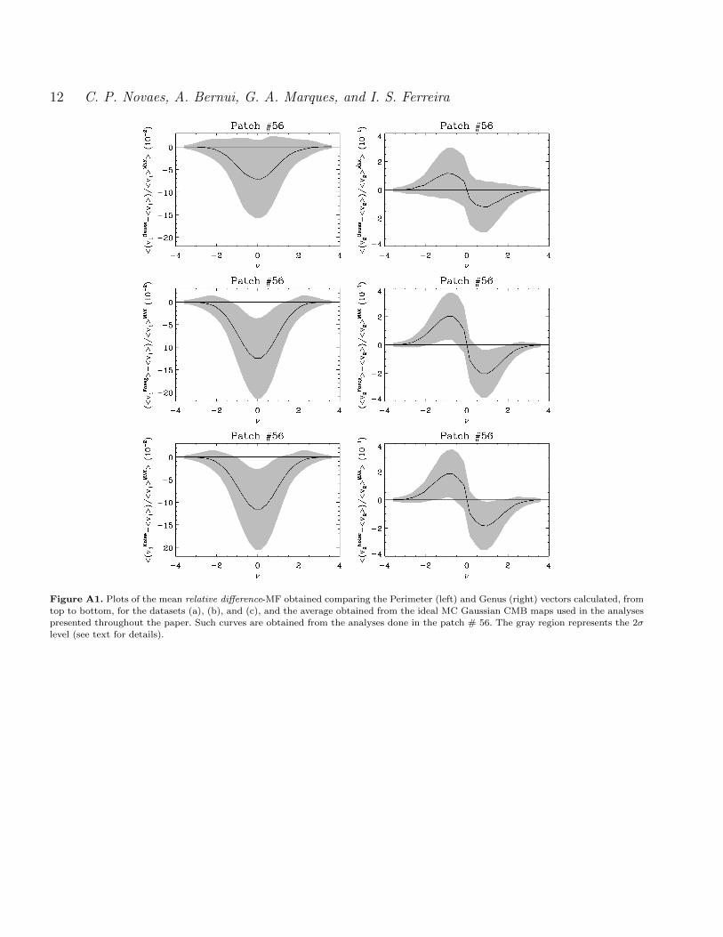
Aiming to support some of our conclusions and propitiatethe reader an easier way to verify our claims, we performedsome additional tests evaluating how the presence of sec-ondary signals and the beam effect would influence our anal-yses. For this we investigate the amplitude and signatureof the relative difference-MF obtained comparing the idealMC Gaussian CMB maps used throughout this paper andthree other sets of synthetic CMB maps. These sets are com-posed by 5000 MC realization each, generated consideringNside = 512, and corresponds to Gaussian CMB maps towhich we add the following effects:

(a) smoothing these MC Gaussian CMB maps with a Gaus-sian beam with fwhm = 5′,(b) adding a residual contribution of foreground emission(as explained below) and a Gaussian beam with fwhm =5′,(c) adding inhomogeneous noise (as explained below) and

a Gaussian beam with fwhm = 5′.

The first set of maps, set (a), is simulated as described inSection 4.1, posteriorly smoothed with the HEALPix Gaus-sian beam of fwhm = 5′. The second one, set (b), is con-structed including the contribution from foreground emis-sion as a residual signal, in an attempt to imitate the possi-ble contents of a Planck data map. Initially, we estimate thecontribution of the most important Galactic foreground sig-nals, namely, the synchrotron, free-free, and dust emission.For this we performed an extrapolation (or interpolation inthe case of the dust emission), pixel by pixel, from a set ofdata maps covering a wide range of frequencies, maps pub-licly available as part of the Planck and WMAP-9yr data

releases (Planck Collaboration 2015c; Bennett et al. 2013).The residual contribution, estimated as being 10% of thefinal template, was then added to the Gaussian MC CMBmaps also, generated as described in Section 4.1. Finally, wehave applied a Gaussian beam of fwhm = 5′ upon thesemaps.

The simulation of the inhomogeneous noise consideredin the set (c) was performed based on what is expected tobe present in the SMICA map. For this we used the noise mapreleased jointly to the SMICA map to estimate the σnoise ineach pixel p as being the standard deviation of the noisevalues from a set of pixels in a disk around p. Multiply-ing the standard deviation map, pixel-by-pixel, by a normaldistribution with zero mean and unitary standard devia-tion we obtain the SMICA-like noise map. The noise map isadded to the Gaussian realizations already convolved witha HEALPix Gaussian beam with fwhm = 5′.

For each map of these three sets we calculate thePerimeter and Genus vectors of the sky region correspond-ing to the patch # 56. This patch was chosen for two rea-sons, namely, its proximity to the Galactic plane and highernoise contribution. The Figure A1 presents the mean relativedifference-MF between the k-th MF obtained from each mapof a given set of realizations and the mean MF calculatedfrom the ideal MC Gaussian CMB maps used throughoutthe analyses of previous sections, 〈vk〉, that is,

〈rel. difference-MFjk〉 ≡

⟨(vjk − 〈vk〉〈vk〉MAX

)∣∣∣∣for the i-th map

⟩,(A1)

where i = 1, ..., 5000, and the index j indicates the data-sets,that is, j = (a), then vj

k = vGauss.k , j = (b), then vj

k = vForeg.

k ,and j = (c), then vj

k = vNoisek . Note from this equation that

the mean curve is the average of the relative difference-MFobtained from the set of MC CMB maps.

This paper has been typeset from a TEX/ LATEX file preparedby the author.

c© 2013 RAS, MNRAS 000, 1–11


1

Figure A1. Plots of the mean relative difference-MF obtained comparing the Perimeter (left) and Genus (right) vectors calculated, fromtop to bottom, for the datasets (a), (b), and (c), and the average obtained from the ideal MC Gaussian CMB maps used in the analyses

presented throughout the paper. Such curves are obtained from the analyses done in the patch # 56. The gray region represents the 2σ

level (see text for details).

c© 2013 RAS, MNRAS 000, 1–11

Local analyses of Planck maps with Minkowski Functionals · Local analyses of Planck maps with...

Documents

Transcript of Local analyses of Planck maps with Minkowski Functionals · Local analyses of Planck maps with...