Load Forecasting

Eugene FeinbergApplied Math & StatisticsStony Brook University

NSF workshop, November 3-4, 2003

Importance of Load Forecasting in Deregulated Markets

Purchasing, generation, sales Contracts Load switching Area planning Infrastructure development/capital

expenditure decision making

Types of Forecasting

S h o rt term fo recas ts(o n e h o u r to a w eek )

M ed iu m fo recas ts(a m o n th u p to a year)

Lo n g term fo recas ts(o ver o n e year)

Load Forecasts

Factors for accurate forecasts

Weather influence

Time factors

Customer classes

Weather Influence

Electric load has an obvious correlation toweather. The most important variables responsible in load changes are: Dry and wet bulb temperature Dew point Humidity Wind Speed / Wind Direction Sky Cover Sunshine

Time factors

In the forecasting model, we should also

consider time factors such as: The day of the week The hour of the day Holidays

Customer Class

Electric utilities usually serve different types of customers such as residential, commercial, and industrial. The following graphs show the load behavior in the above classes by showing the amount of peak load per customer, and the total energy.

Load Curves

Mathematical Methods

Regression models Similar day approach Statistical learning models Neural networks

Our Work

Our research group has developed statistical learning models for long

term forecasting (2-3 years ahead) and

shortterm forecasting (48 hours ahead).

Long Term Forecasting

The focus of this project was to forecast theannual peak demand for distributionsubstations and feeders.

Annual peak load is the value most important

to area planning, since peak load most strongly

impacts capacity requirements.

Model Description

The proposed method models electric powerdemand for close geographic areas, load pocketsduring the summer period. The model takes intoaccount: Weather parameters (temperature, humidity, sky

cover, wind speed, and sunshine). Day of the week and an hour during the day.

Model

A multiplicative model of the following form was developed

L(t)=L(d(t),h(t))f(w(t))+R(t)where: L(d(t),h(t)) is the daily and hourly component

L(t) is the original load f(w(t)) is the weather factor R(t) is the random error

Model Cont:E l e c t r i c l o a d d e p e n d s :

o n t h e c u r r e n t w e a t h e r c o n d i t i o n s w e a t h e r d u r i n g l a s t h o u r s a n d d a y s .

T h e r e g r e s s i o n m o d e l u s e d i s

,

,,0i

titiw Xft

w h e r e X i , t - a r e n o n - l i n e a r f u n c t i o n s o f t h e a p p r o p r i a t e w e a t h e r p a r a m e t e r s .

Computational Results

The performance of proposed method was evaluatedfrom the graphs of the weather normalized load profiles and actual load profiles and from the followingfour statistical characteristics: Scatter plot of the actual load versus the model. Correlation between the actual load and the model. R- square between the actual load and the model. Normalized distance between the actual load and the

model.

Scatter Plot of the Actual LoadVs the Model

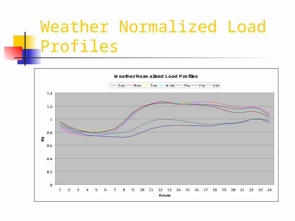
Weather Normalized Load Profiles

Weather Normalized Load Profiles

0

0.2

0.4

0.6

0.8

1

1.2

1.4

1 2 3 4 5 6 7 8 9 10 11 12 13 14 15 16 17 18 19 20 21 22 23 24

Hours

MW

Sun Mon Tue Wed Thu Fri Sat

Actual Load Profiles

Actual Load Profiles

0

50

100

150

200

250

300

350

400

1 2 3 4 5 6 7 8 9 10 11 12 13 14 15 16 17 18 19 20 21 22 23 24

Hours

MW

Sun Mon Tue Wed Thu Fri Sat

Correlation Between the Actual Load and the Model

Correlation between the Actual Load and the Model

0.955

0.96

0.965

0.97

0.975

0.98

0.985

0.99

1 2 3 4 5 6 7 8 9 10

Iteration

Co

rrela

tio

n

R-square Between the ActualLoad and the Model

Regression Output : R2

(defined as the proportion of variance of the response that is predictable from the regressor variables)

0

0.1

0.2

0.3

0.4

0.5

0.6

0.7

0.8

0.9

1

1 2 3 4 5 6 7 8 9 10

Iteration

R2

Normalized Distance Betweenthe Actual Load Vs the Model

Normalized Distance between the Actual Load and the Model

0

0.05

0.1

0.15

0.2

0.25

0.3

1 2 3 4 5 6 7 8 9 10

Iteration

Dis

tan

ce

Short Term Forecasting

The focus of the project was to provideload pocket forecasting (up to 48 hoursahead) and transformer ratings.

We adjust the algorithm developed for long

term forecasting to produce results forshort term forecasting.

Short Term Load Forecasting