LOAD FLOW AND CONTINGENCY ANALYSIS USING …dsresearchcenter.net/PDF/V1_I9/V1-I9-11.pdf · Ybus...

LAKSHMISWARUPA M, et al, International Journal of Computers Electrical and Advanced Communication Engineering [IJCEACE]TM Volume 1, Issue 9, PP: 126 - 134, JAN - JUL’ 2016.

International Journal of Computers Electrical and Advanced Communications Engineering Vol.1 (9), ISSN: 2250-3129, JAN – JUL’ 2016 PP: 126 - 134

LOAD FLOW AND CONTINGENCY ANALYSIS USING

NEPLAN SOFTWARE

Dr .M. LAKSHMISWARUPA 1*, Mr. D. RAMESH 2*

1. Professor -Dept of EEE, Malla Reddy Engg. College (AUTONOMOUS), Hyderabad, India.

2. Asst. Prof- Dept of EEE, Malla Reddy Engg. College (AUTONOMOUS), Hyderabad, India.

Abstract— Load flow analysis is an important method for the power system analysis and designing. This analysis is carried out at each

and every state of planning, operation, control and economic scheduling. In this project, firstly we have analyzed IEEE-14 bus system

under the standard test data & after that we have increased load data in step of 5%. For finding a most sensitive node, the results are

compared with the original power flow results of IEEE-14 bus system. According to the reasons that are mentioned, the prediction and

recognition of voltage instability in power system has particular importance and it makes the network security stronger. In this paper,

we have focus on the finding of most sensitive node in IEEE-14 bus systems. Simulation is carried out at NEPLAN software which

includes a complete set of user-friendly graphical interface for voltage stability analysis and sensitive nodes determination. This project

also includes power system contingencies based on the maximum loading parameter point in order to analyze the voltage stability using

continuation power flow method.

Index Terms— IEEE-14 Bus, System, Sensitive Node, Contingency ranking, Continuation Power Flow, Voltage Stability.

I. INTRODUCTION

The voltage stability is the capability of a power system to

maintain steady state voltage at all buses in the system at

normal values and after being subjected to a disturbance [1]. A

power system becomes unstable, when voltages

uncontrollably changes due to the disbalance between load

and generation, outage of equipment & lines and failure of

voltage control mechanism in the system. The problem of

voltage instability occurs mainly due to deficient supply of the

reactive power or by an unnecessary absorption of reactive

power. Continuous monitoring of the system status is required

because the voltage instability affects the satisfactory

operation of power system. Voltage stability assessment [1,2]

is becoming an essential task for power system planning and

operation. Power system security analysis [3] forms an

integral part of modern energy management system. Security

is a term used to reflect a power system’s ability to meets its

load without unduly stressing its apparatus or allowing

variables to stray from prescribed range under the apparatus or

allowing variables to stray from prescribed range under certain

pre-specified credible contingencies. The contingencies [4,5]

are in the form of network outage such as line or transformer

outage or in the form of equipment outage e.g. a generator

outage. The outages, which are important from limit violation

viewpoint, are branch flow for line security or MW security

and bus voltage magnitude for voltage security. Voltage

stability has become a very important limit in assessing

voltage security.

The importance of voltage stability in determining system

security and performance will continue to increase due to the

increased loadings and interconnections brought about by

economic and environmental pressures which have let to

increasingly complex power systems that must operate closer

to their stability limits.

II. METHODLOGY

A. Contingency Analysis Studies

The most difficult methodological problem to cope within

contingency analysis is the accuracy of the method and the

speed of solution of the model used. The operator usually

needs to know if the present operation of the system is secure

and what will happen if a particular outage occurs. Operations

personnel must recognize which line or generator outages will

cause power flows or voltages to go out of their limits. In order

to predict the effects of outages, contingency analysis

technique is used. Contingency analysis procedures model a

single equipment failure event, that is one line or one generator

outage, or multiple equipment failure events, that is two

transmission lines, a transmission line and a generator; one

after another in sequence until all credible outages have been

studied. For each outage tested, the contingency analysis

procedure checks all power flows and voltage levels in the

network against their respective limits [3].

B. Methods of Contingency Analysis

Methods based on AC power flow calculations are

considered to be deterministic methods which are accurate

compared to DC power flow methods.[1] The methods used for

analyzing the contingencies are based on full AC load flow

analysis are faster and accurate. And therefore the wide use of

the network control center. Because the contingency alarms

came too late for operators to act, they are worthless. Most

operations control centers that use an AC power flow program

for contingency analysis use either a Newton-Raphson or the

decoupled power flow. An algorithm under the AC load flow

method will be used to ensure higher accuracy [2]. Since these

algorithms has a good performance in terms of convergence

speed and reliability in unfavorable conditions. Below is a brief

description of these methods.



C. Equations

The programming of the above procedure for contingency

analysis has been implemented in NEPLAN is fast decoupled

load flow. And more a set of single and multiple contingencies

are performed on Azerbaijan power network using full AC load

flow analysis applying the simulation of lines and generator's

outage. The simulation of transmission line outage is carried

out by the formulation of the corresponding admittance matrix.

Assume that the line connected between buses m and n will be

outage. The elements of the admittance [Y] matrix that will be

affected are ، ، and , and the new values of those admittances

for the (π) mode of representation of transmission lines will be

given by:

III. SOFTWARE DESCRIPTION

MATLAB is a programming language developed by MathWorks. It started out as a matrix programming language

where linear algebra programming was simple. It can be run

both under interactive sessions and as a batch job.

This tutorial gives you aggressively a gentle introduction of

MATLAB programming language. It is designed to give

students fluency in MATLAB programming language.

Problem-based MATLAB examples have been given in

simple and easy way to make your learning fast and effective.

NEPLAN software is the best software of this feature

because its Background is based on the power market.

The characteristic of voltage stability are illustrated with IEEE

14-bus system. The generator produces active power, which is

transferred through a transmission line to laod.The reactive

power capability of the generator is infinite. Thus the

generator terminal voltage V1 is constant.

Fig 1: Line diagram of IEEE bus test system

V2 = √ ((V12 -2QX) ± √ ( V1

4 -4QXV12 -4PX2 )) 2

Pi = ΣViVjYij cos(δi – δijYij)

Qi = ΣViVjYij sin(δi – δijYij)

For i,j =1 to n

Where Pi and Qi are active and reactive powers injected at

load.

Fourteen Bus system

Continuous

powergui

A B C

a b c

A B C

a b c

A B C

a b c

A B C

a b c

A B C

a b c

A B C

A B CA B CA B CA B C

A

B

C

A B C

A B C

A

B

C

A B C

A B C

A

B

C

A

B

C

A

B

C

A

B

C

A

B

C

A

B

C

A

B

C

A

B

C

A

B

C

A

B

C

A

B

C

A

B

C

A

B

C

A

B

C

A

B

C

A

B

C

A

B

C

A

B

C

A

B

C

A

B

C

A B C

A B C

A

B

C

A

B

C

A

B

C

A

B

C

A

B

C

A

B

C

A

B

C

A

B

C

A

B

C

A

B

C

A B C

A B C

A

B

C

A

B

C

A

B

C

A

B

C

A

B

C

A

B

C

A B C

Synchronous

Compensator

A B C

Synchronous

Compensator

A B C

Synchronous

Compensator

Vabc

Iabc

A B Ca b cBus 9

Bus 9

Vabc

Iabc

A B Ca b cBus 8

Bus 8

Vabc

Iabc

A B Ca b cBus 7

Bus 7

Vabc

Iabc

A B Ca b cBus 6

Bus 6

Vabc

Iabc

A B Ca b cBus 5

Bus 5

Vabc

Iabc

A B Ca b cBus 4

Bus 4

Vabc

Iabc

A B Ca b cBus 3

Bus 3

Vabc

Iabc

A B Ca b cBus 2

Bus 2

Vabc

Iabc

A B Ca b cBus 14

Bus 14

Vabc

Iabc

A B Ca b cBus 13

Bus 13

Vabc

Iabc

A B Ca b cBus 12

Bus 12

Vabc

Iabc

A B Ca b cBus 11

Bus 11

Vabc

Iabc

A B Ca b cBus 10

Bus 10

Vabc

Iabc

A B Ca b cBus 1

Bus 1

A B C

Generator1

A B C

Generator

Fig 2. Simulation Model for IEEE 14-BUS system

(Healthy condition)

Time (secs)

Voltage at

buses (P.u)



Fig 3. Results of Three –Phase Voltages for Healthy

condition

Fig 4. Ybus formation

Fig 5. Line data of IEEE 14-bus system

Fig 6 Eigen values of the reduced Jacobian matrix

against load multiplication factor, K.

Table 1.1: Transmission lines data (R, X and B in Pu on

100MVA base) for the 14-bus test system

End buses R X B/2

1-2 0.01938 0.05917 0.0264

2-4 0.05811 0.17632 0.0170

12-13 0.22092 0.19988 0

13-14 0.17093 0.34802 0

Table 1.2: Transformer data (R, X in pu on 100 MVA base)

for the 14-bus test system

End buses R X

3-8 0.0671 0.17173

7-9 0 0.11001

6-7 0 0.2522

Table 1.3: Shunt capacitor(R, X in pu on 100 MVA base) for

the 14-bus test system

Table 1.4: Base case load data (Pu on 100 MVA base) for the

14-bus test system

Table 1.5: Base case generator data (Pu on 100 MVA base) for

the 14-bus test system

End buses MVAR(pu)

4 0.191

5 0.016

bus P(MW) QMVAR(pu)

3 0.217 0.127

4 0.942 0.191

7 0.112 0.075

8 0.050 0

9 0.295 0.166

10 0.09 0.058

11 0.035 0.018

12 0.061 0.016

13 0.135 0.058

14 0.1499 0.050



Table 1.6:

Eigen values of reduced Jacobian matrix (Pu on 100 MVA

base) for the 14-bus test system

K E1 E2 E3 E4

1.124 0.1861 0.3190 0.1361 0.5786

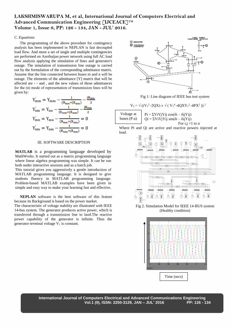
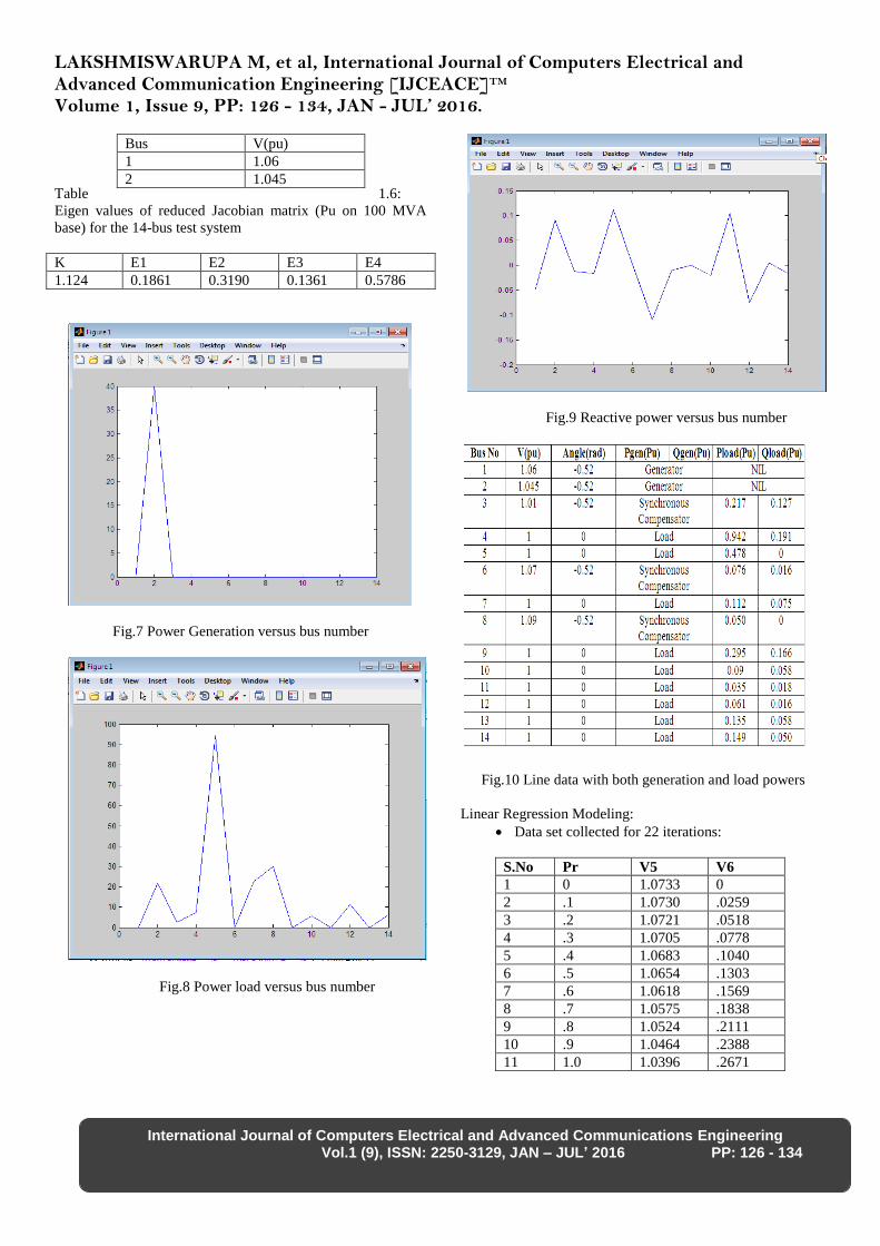
Fig.7 Power Generation versus bus number

Fig.8 Power load versus bus number

Fig.9 Reactive power versus bus number

Fig.10 Line data with both generation and load powers

Linear Regression Modeling:

Data set collected for 22 iterations:

S.No Pr V5 V6

1 0 1.0733 0

2 .1 1.0730 .0259

3 .2 1.0721 .0518

4 .3 1.0705 .0778

5 .4 1.0683 .1040

6 .5 1.0654 .1303

7 .6 1.0618 .1569

8 .7 1.0575 .1838

9 .8 1.0524 .2111

10 .9 1.0464 .2388

11 1.0 1.0396 .2671

Bus V(pu)

1 1.06

2 1.045



12 1.1 1.0317 .2961

13 1.2 1.0227 .3258

14 1.3 1.0124 .3566

15 1.4 1.0005 .3885

16 1.5 .9868 .4576

17 1.6 .9769 .4220

18 1.7 .9519 .4959

19 1.8 ,.9286 .5382

20 1.9 .8984 .5872

21 2.0 .8538 .6504

22 2.1 .7613 .7613

Fig.11: Loading Factor K=0.5

Fig.12. Loading factor K= 0.9

Fig. 13: Loading Factor K=1

Fig.14. Loading Factor K=1.1

Fig.15. P-V curve at weakest buses for different

iterations

Fitness Equation:



Fig.16. Linear regression (Basic fitting) Analysis

(K=1.146)

Fig.17 Data statistics of mean, standard deviation

Fig.18. Data Statistics for Input

Fig. 19. Data Statistics for Output

Simulation model in NEPLAN Software:

Fig.20: Selection of Method for Load Flow



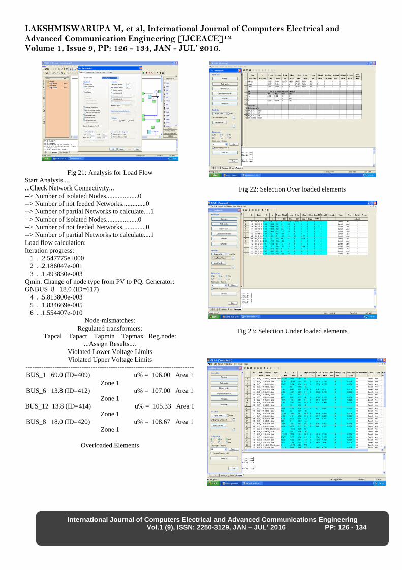
Fig 21: Analysis for Load Flow

Start Analysis....

...Check Network Connectivity...

--> Number of isolated Nodes...................0

--> Number of not feeded Networks..............0

--> Number of partial Networks to calculate....1




Load flow calculation:

Iteration progress:

1 . .2.547775e+000

2 . .2.186047e-001

3 . .1.493830e-003

Qmin. Change of node type from PV to PQ. Generator:

GNBUS_8 18.0 (ID=617)

4 . .5.813800e-003

5 . .1.834669e-005

6 . .1.554407e-010

Node-mismatches:

Regulated transformers:

Tapcal Tapact Tapmin Tapmax Reg.node:

...Assign Results....

Violated Lower Voltage Limits

Violated Upper Voltage Limits

---------------------------------------------------------------------------

BUS_1 69.0 (ID=409) u% = 106.00 Area 1

Zone 1

BUS_6 13.8 (ID=412) u% = 107.00 Area 1

Zone 1

BUS_12 13.8 (ID=414) u% = 105.33 Area 1

Zone 1

BUS_8 18.0 (ID=420) u% = 108.67 Area 1

Zone 1

Overloaded Elements

Fig 22: Selection Over loaded elements

Fig 23: Selection Under loaded elements



Fig 24: Selection of all elements

Fig 25: Selection of elements with their voltage profile,

powers

Building Network Started...

...Check Network Connectivity...

...Update partial Networks...




--Building Network Completed

Optimal Power Flow calculation...

Call: 1 - Feas./Opt. error = 7.868067e-001/3.228385e-002










--- Value of Objective function = 1.381108e-002


























EXIT OPF: *** LOCALLY OPTIMAL SOLUTION FOUND

***

Obj. = 2.37387966

Network MW losses = 2.37387966

Network Mvar losses = -16.06956110

Network Total Gen.Cost (CurrU/h) = 0.00000000

Voltage Deviation^2 (%) = 0.00000000

Discretizing variables..

...Assign Results....

Violated Lower Voltage Limits

Violated Upper Voltage Limits

Overloaded Elements

Completed

Fig 26: Load flow, state estimation and contingency analysis

completed

IV. CONCLUSIONS

In this paper, the method for load flow, state estimation and

contingency analysis was done using NEPLAN software was

proposed. The proposed algorithm has been applied to

practical IEEE 14-Bus system. The study of contingency

ranking and analysis is very important from the view point of

power system security. Here obtained results lead the

contingency ranking for IEEE 14 Bus system. For IEEE-14

Bus system line number 10 connected between Bus 7 to Bus 9

is most severe line among all 20 lines. This identification

being able to significantly improve the secure performance of



power systems and to reduce the chances of failure of system.

Good planning helps to ensure that reliability and security of

the system. Contingency ranking analysis helps the power

system engineer to give the most priority to notice or

monitoring the line flows to which line and monitoring other

lines flow in descending order. The fitness value of the

objective function is obtained in more optimized way in

NEPLAN software than compared to MATLAB software.

V. REFERENCES [1]. A.J. Wood and Wollenberg, “Power generation, operation

and control,”2nd Edition, John and Wiley & Sons Ltd, 2009.

[2] B. Scott, O.Alsac and A.J Monticelli, “Security analysis

and optimization,” Proceedings of the IEEE, Vol.75, No.12,

Dec1987,pp.1623-1644.

[3] N.M. Peterson W.F. Tinney and D.W. Bree, “Iterative

linear AC power flow for fast approximate outage studies,

“IEEE Transactions on Power Apparatus and Systems, Vol.91,

No. 5, October 1972, pp.2048-2058.

[4] Ching-Yin Lee and Nanming Chen, “Distribution factors

of reactive power flow in transmission line and transformer

outage studies, “IEEE Transactions on Power Systems, Vol. 7,

No.1, February 1992, pp. 194-200.M. Young, The Technical

Writer’s Handbook. Mill Valley,CA: University Science,1989.

[5] S.N. Singh and S.C. Srivastava,”Improved voltage and

reactive power distribution for outage studies, “IEEE

Transactions on Power Systems, Vol.12, No.3, August 1997,

pp.1085- 1093

[6] J. Zaborsky, K.W. Whang, K. Prasad, Fast contingency

evaluation using concentric relaxation, IEEE Transactions on

Power Apparatus and Systems,Vol. PAS-99, No.1,

January1980, pp. 28–36.

[7] R. Bacher, W.F. Tinney, "Faster local power flow

solutions: the zero mismatch approach," IEEE Transactions on

Power Systems, Vol. 4, No. 4, October 1989, pp. 1345- 1354.

[8] P. Marannino, A. Berizzi, M. Merlo, G. Demartini, “A

Rule-based Fuzzy Logic Approach for the Voltage collapse

Risk Classification”, IEEE Power Engineering Society Winter

Meeting, Vol. 2 , pp. 876-881,2002.

[9]. Tarlochan S Sindhu and Lan Chui, “Contingency

Screening for Steady State Security Analysis by using FFT

and Artificial Neural Networks”, IEEE Transactions on Power

Systems, Vol. 15, No. 1, February 2000.

LOAD FLOW AND CONTINGENCY ANALYSIS USING …dsresearchcenter.net/PDF/V1_I9/V1-I9-11.pdf · Ybus...

Documents

Transcript of LOAD FLOW AND CONTINGENCY ANALYSIS USING …dsresearchcenter.net/PDF/V1_I9/V1-I9-11.pdf · Ybus...