Discovering Non-linear Ranking Functions bySolving Semi-algebraic Systems�

Yinghua Chen1, Bican Xia1, Lu Yang2, Naijun Zhan ��,3, and Chaochen Zhou3

1 LMAM & School of Mathematical Sciences, Peking University2 Institute of Theoretical Computing,, East China Normal University

3 Lab. of Computer Science, Institute of Software, Chinese Academy of Sciences

Abstract. Differing from [6] this paper reduces non-linear ranking func-tion discovering for polynomial programs to semi-algebraic system solv-ing, and demonstrates how to apply the symbolic computation tools,DISCOVERER and QEPCAD, to some interesting examples.

Keywords: Program Verification, Loop Termination, Ranking Function,Polynomial Programs, Semi-Algebraic Systems, Computer Algebra, DIS-COVERER, QEPCAD.

1 Introduction

The design of reliable software is a grand challenge in computer science [17] in the21st century, as our modern life becomes more and more computerized. One of thebases for designing reliable software is the correctness of programs. The dominantapproach to automatic program verification is the so-calledFloyd-Hoare-Dijkstra’sinductive assertion method [8,10,11], by using pre- and post- conditions, loop in-variants and proving loop termination through ranking functions, etc. Therefore,the discovery of loop invariants and ranking functions plays a central role in prov-ing the correctness of programs and is also thought of as the most challenging partof the approach.

The classical method for establishing termination of a program is the useof well-founded domain together with so-called ranking function that maps thestate space of the program to the domain. Termination is then concluded bydemonstrating that each step as the program moves forwards decreases the mea-sure assigned by the ranking function. As there can be no infinite descendingchain of elements in a well-founded domain, any execution of the program musteventually terminate. Clearly, the existence of such a ranking function for anygiven program implies its termination. Recently, the synthesis of ranking func-tions draws increasing attention, and some heuristics concerning how to automat-ically generate linear ranking functions for linear programs have been proposed� The work is in part supported by the projects NKBRPC-2002cb312200,

2004CB318003, 2005CB321902, and NSFC-60493200, 60421001, 60573007.�� The corresponding author: South Fourth Street, No. 4, Zhong Guan Cun, Beijing,

100080, P.R. China, znj@ios.ac.cn

C.B. Jones, Z. Liu, J. Woodcock (Eds.): ICTAC 2007, LNCS 4711, pp. 34–49, 2007.c© Springer-Verlag Berlin Heidelberg 2007

Discovering Non-linear Ranking Functions 35

[7,5,13]. [7] proposed a heuristic strategy to synthesize a linear ranking functionaccording to the syntax of a linear program. Since in many cases there doesnot exist obvious correlation between the syntax of a program and its rankingfunctions, this approach is very restrictive. Notably, [5] utilized the theory ofpolyhedra to synthesize linear ranking function of linear programs, and [13] firstpresented a complete method to find out linear ranking functions for a class oflinear programs that have only single path without nested loop, in the sensethat if there exists a linear ranking function for a program in the class, then themethod can eventually discover it.

Existence of ranking function is only a sufficient condition on the terminationof a program. It is easy to construct programs that terminate, but have no rankingfunctions. Furthermore, even if a (linear) programhas ranking functions, itmaynothave a linear ranking function. we will show this point by an example later in thepaper. Besides, it is well-known that the termination of programs is undecidablein general, even for the class of linear programs [16] or a simple class of polynomialprograms [2]. In contrast to the above approach, [16,1] tried to identify decidablesubclasses andproved the decidability of the terminationproblem for a special classof linear programs over reals and integers, respectively. [27] further developed thework of [16] by calculating symbolic (sufficient) conditions for the termination ofits subclasses through computer algebra tool, DISCOVERER.

Linear programs with linear ranking functions compose a very small classof programs. As to polynomial programs, [2] proposed an incomplete method todecide whether a polynomial program terminates by using the technique of finitedifference tree. However, [2] can only tackle very simple polynomial programs,that have ‘polynomial behaviour’.

In 2005, [6] presented a very general approach to ranking function discoveryas well as invariant generation of polynomial programs by parametric abstrac-tion, Lagrangian relaxation and semidefinite programming. The basic idea ofthe approach is: first the program semantics is expressed in polynomial form;then the unknown ranking function and invariants are abstracted in paramet-ric form; the verification conditions are abstracted as numerical constraints ofthe parameters through Lagrangian relaxation; the remaining universal quan-tifications are handled by semidefinite programming; finally the parameters arecomputed using semidefinite programming solvers. [6] does not directly use thefirst-order quantifier elimination method due to its bad complexity of doubly ex-ponential1. Therefore the approach of [6] is incomplete in the sense that for someprogram that may have ranking functions and invariants of the predefined form,however applying the approach cannot find them, as Lagrangian relaxation andover-approximation of the positive semi-definiteness of a polynomial are applied.

We here use semi-algebraic transition system (SATS), which is an extensionof algebraic transition systems in [14], to represent polynomial programs. Then,for a loop in a given SATS (i.e. a given polynomial program), we can first assume

1 [6] does not provide information about complexity of its own approach. But we areafraid that the complexity of the semidefinite programming, in particular, when theGram Matrix method is involved, is also bad.

36 Y. Chen et al.

to be a ranking function a polynomial in its program variables with parametriccoefficients. In order to determine the parameters, we translate the definition ofranking functions in regard with the predefined polynomial into several SASs,and prove that the polynomial is a ranking function of the loop if and only ifeach of these SASs has no real solutions. After the translation we apply the func-tions of root classification for parametric SASs [22,23,24] (and real root isolationfor constant SASs [20] if needed) of DISCOVERER to each of these SASs togenerate conditions on the parameters. If some universally quantified programvariables remain in the resulted conditions, in order to acquire a condition onlyon the parameters, we can apply QEPCAD to eliminate the remaining quan-tifiers. In case that the final condition on parameters is still very complicated,applying PCAD (partial cylindrical algebra decomposition [4]) included in bothDISCOVERER and QEPCAD, we can conclude whether the condition can besatisfied. If yes, we can further apply PCAD to get the instantiations of theseparameters, and therefore achieve a specific polynomial ranking function as nec-essary. If not, we can define another polynomial template and repeat the aboveprocedure. So our approach does not compromise its completeness. As to thecomplexity of the approach, DISCOVERER functions on root classification andreal root isolation for SASs include algorithms, such as Wu’s triangularization[18], to eliminate variables through equalities in SASs with a cost of singly ex-ponential in the number of variables and parameters. Hence, the application ofthese algorithms can dramatically ease the application of other algorithms ofDISCOVERER, QEPCAD and/or PCAD, although they still cost doubly ex-ponential but in the number of remaining variables and parameters. A detailedanalysis of the complexity will be published in a later paper. In this paper, bybriefing the theories behind DISCOVERER we show why the tool works andby applying to examples we show how the tool discovers ranking functions forpolynomial programs.

The rest of this paper is structured as follows: Section 2 presents a brief reviewof the theories and tools of semi-algebraic systems, in particular, the theories onroot classification of parametric semi-algebraic systems and on real root isola-tion of constant SASs, and their implementations in the computer algebra toolDISCOVERER; We extend the notion of algebraic transition systems of [14] tosemi-algebraic transition system to represent polynomial programs in Section3; In Section 4, we use examples to illustrate the reduction of non-linear rank-ing function discovering to SAS solving; and Section 5 draws a summary anddiscusses future work.

2 Theories and Tools on Solving Semi-algebraic Systems

In this section, we introduce the theories and the tool DISCOVERER 2 onsolving SASs.

2 DISCOVERER can be downloaded at http://www.is.pku.edu.cn/∼xbc/ discoverer.html

Discovering Non-linear Ranking Functions 37

2.1 Semi-algebraic Systems

Let K be a field, X = {x1, · · · , xn} a set of indeterminates, and K[x1, ..., xn] thering of polynomials in the n indeterminates with coefficients in K, ranged overp(x1, . . . , xn) with possible subscription and superscription. Let the variables beordered as x1 ≺ x2 ≺ · · · ≺ xn. Then, the leading variable of a polynomial p is thevariable with the biggest index which indeed occurs in p. If the leading vari-able of a polynomial p is xk, p can be collected w.r.t its leading variable asp = cmxm

k + · · · + c0 where m is the degree of p w.r.t. xk and cis are polynomialsin K[x1, ..., xk−1]. We call cmxm

k the leading term of p w.r.t. xk and cm the lead-ing coefficient. For example, let p(x1, . . . , x5) = x6

2x3 + 2x41x

44 + (3x2x3 + x1)x5

4, so,its leading variable, term and coefficient are x4, (3x2x3 + x1)x5

4 and 3x2x3 + x1,respectively.

Anatomic polynomial formula over K[x1, ..., xn] is of the form p(x1, . . . , xn) � 0,where � ∈ {=, >, ≥, �=}, while a polynomial formula over K[x1, ..., xn] is constructedfrom atomic polynomial formulae by applying the logical connectives. Conjunc-tive polynomial formulae are those that are built from atomic polynomial formulaewith the logical operator ∧. We will denote by PF ({x1, . . . , xn}) the set of polyno-mial formulae and by CPF ({x1, . . . , xn}) the set of conjunctive polynomial formu-lae, respectively.

In what follows, we will use Q to stand for rationales and R for reals, and fixK to be Q. In fact, all results discussed below can be applied to R.

In the following, the n indeterminates are divided into two groups: u =(u1, ..., ud) and x = (x1, ..., xs), which are called parameters and variables, re-spectively, and we sometimes use “,” to denote the conjunction of atomic for-mulae for simplicity.

Definition 1. A semi-algebraic system is a conjunctive polynomial formula ofthe following form: ������

�����

p1(u,x) = 0, ..., pr(u,x) = 0,

g1(u,x) ≥ 0, ..., gk(u,x) ≥ 0,gk+1(u,x) > 0, ..., gt(u,x) > 0,h1(u, x) �= 0, ..., hm(u,x) �= 0,

(1)

where r > 1, t ≥ k ≥ 0, m ≥ 0 and all pi’s, gi’s and hi’s are in Q[u,x] \ Q. An SASof the form (1) is called parametric if d �= 0, otherwise constant.

An SAS of the form (1) is usually denoted by a quadruple [P, G1, G2, H], whereP = [p1, ..., pr], G1 = [g1, ..., gk], G2 = [gk+1, ..., gt] and H = [h1, ..., hm].

For a constant SAS S, interesting questions are how to compute the numberof real solutions of S, and if the number is finite, how to compute these realsolutions. For a parametric SAS, the interesting problem is so-called real solutionclassification, that is to determine the condition on the parameters such that thesystem has the prescribed number of distinct real solutions, possibly infinite.

38 Y. Chen et al.

2.2 Real Solution Classification

In this subsection, we give a sketch of our theory for real root classification ofparametric SASs. For details, please be referred to [23,26].

A finite set of polynomials T : [T1, ..., Tk] is called a triangular set if it is inthe following form

T1 = T1(x1, ..., xi1),

T2 = T2(x1, ..., xi1 , ..., xi2),

· · · · · ·Tk = Tk(x1, ..., xi1 , ..., xi2 , ..., xik),

where xi is the leading variable of Ti and x1 � xi1 ≺ xi2 ≺ · · · ≺ xik � xs. For anygiven SAS S in the form of (1), where the variables in the order x1 ≺ · · · ≺ xs andall polynomials in S are viewed as polynomials in Q(u)[x], we first decomposethe equations in S into triangular sets, that is, we transform the polynomialset P = [p1, ..., pr] into a finite set T = {T1, ..., Te} where each Ti is a triangularset. Furthermore, this decomposition satisfies Zero(P) =

�ei=1 Zero(Ti/Ji), where

Zero(P) denotes the set of common zeros (in some extension of the field of rationalnumbers) of p1, ..., pr, Zero(Ti/Ji) = Zero(Ti) \ Zero({Ji}), where Ji is the productof leading coefficients of the polynomials in Ti for each i. It is well-known thatthe decomposition can be realized by some triangularization methods such asWu’s method [18].

Example 1. Consider an SAS RS : [P, G1, G2, H] in Q[a, x, y, z] with P = [p1, p2, p3],G1 = [a − 1], G2 = ∅, H = ∅, where

p1 = x2 + y2 − xy − 1, p2 = y2 + z2 − yz − a2, p3 = z2 + x2 − zx − 1,

The equations P can be decomposed into three triangular sets in Q(a)[x, y, z]

T1 : [x2 − ax + a2 − 1, y − a, z − a],T2 : [x2 + ax + a2 − 1, y + a, z + a],T3 : [2x2 + a2 − 3, 2y(x − y) + a2 − 1, (x − y)z + xy − 1].

To simplify our description, let us suppose the number of polynomials in eachtriangular set is equal to the number of variables as in the above example. Fordiscussion on the other cases of T , please be referred to [19]. That is to say, wenow only consider triangular system

���������

f1(u, x1) = 0,...

fs(u, x1, ..., xs) = 0,G1, G2, H.

(2)

Second, we compute a so-called border polynomial from the resulting systems[Ti, G1, G2, H]. We need to introduce some concepts. Suppose F and G are poly-nomials in x with degrees m and l, respectively. Thus, they can be written in thefollowing forms

F = a0xm + a1x

m−1 + · · · + am−1x + am, G = b0xl + b1x

l−1 + · · · + bl−1x + bl.

Discovering Non-linear Ranking Functions 39

The following (m + l) × (m + l) matrix (those entries except ai, bj are all zero)

��������������

a0 a1 · · · ama0 a1 · · · am

. . .. . .

. . .a0 a1 · · · am

b0 b1 · · · bl

b0 b1 · · · bl

. . .. . .

. . .b0 b1 · · · bl

�

��� ��� l

��� ���m

,

is called the Sylvester matrix of F and G with respect to x. The determinant ofthe matrix is called the Sylvester resultant or resultant of F and G with respectto x and is denoted by res(F, G, x).

For system (2), we compute the resultant of fs and f ′s w.r.t. xs and denote it

by dis(fs) (it has the leading coefficient and discriminant of fs as factors). Then wecompute the successive resultant of dis(fs) and the triangular set {fs−1, ..., f1}. Thatis, we compute res(res(· · · res(res(dis(fs), fs−1, xs−1), fs−2, xs−2) · · · ), f1, x1) and de-note it by res(dis(fs); fs−1, ..., f1) or simply Rs. Similarly, for each i (1 < i ≤ s), wecompute Ri = res(dis(fi); fi−1, ..., f1) and R1 = dis(f1).

For each of those inequalities and inequations, we compute the successiveresultant of gj (or hj) w.r.t. the triangular set [f1, ..., fs] and denote it by Qj

(resp. Qt+j).

Definition 2. For an SAS T as defined by (2), the border polynomial of T is

BP =s�

i=1

Ri

t+m�j=1

Qj .

Sometimes, with a little abuse of notation, we also use BP to denote the square-free part or the set of square-free factors of BP .

Example 2. For the system RS in Example 1, the border polynomial is

BP = a(a − 1)(a + 1)(a2 − 3)(3a2 − 4)(3a2 − 1).

From the result in [23,26], we may assume BP �≡ 0. In fact, if any factor of BP isa zero polynomial, we can further decompose the system into new systems withsuch a property. For a parametric SAS, its border polynomial is a polynomial inthe parameters with the following property.

Theorem 1. Suppose S is a parametric SAS as defined by (2) and BP its borderpolynomial. Then, in each connected component of the complement of BP = 0 inparametric space Rd, the number of distinct real solutions of S is constant.

Third, BP = 0 decomposes the parametric space into a finite number of con-nected region. We then choose sample points in each connected component ofthe complement of BP = 0 and compute the number of distinct real solutions ofS at each sample point. Note that sample points can be obtained by the partialcylindrical algebra decomposition (PCAD) algorithm [4].

40 Y. Chen et al.

Example 3. For the system RS in Example 1, BP = 0 gives a = 0, ± 1, ±√3

3 , ± 2√

33 , ±

√3. The reals are divided into several open intervals by these

points. Because a ≥ 1, we only need to choose, for example, 9/8, 3/2 and 2 from(1,

√3

3 ), (√

33 , 2

√3

3 ) and ( 2√

33 ,

√3), respectively. Then, we substitute each of the

three values for a in the system, and compute the number of distinct real solu-tions of the system, consequently obtain the system has respectively 8, 4 and 0distinct real solutions.

The above three steps constitute the main part of the algorithm in [23,26,19],which, for any input SAS S, outputs the so-called border polynomial BP and aquantifier-free formula Ψ in terms of polynomials in parameters u (and possiblesome variables) such that, provided BP �= 0, Ψ is the necessary and sufficientcondition for S to have the given number (possibly infinite) of real solutions.

Finally, if we want to discuss the case when parameters are on the “boundary”BP = 0, we put BP = 0 (or some of its factors) into the system and apply asimilar procedure to handle the new SAS.

Example 4. By the steps described above, we obtain the necessary and sufficientcondition for RS to have 4 distinct real solutions is 3a2 − 4 > 0 ∧ a2 − 3 < 0provided BP �= 0. Now, if 3a2 − 4 = 0, adding the equation into the system, weobtain a new SAS [ [3a2 − 4, p1, p2, p3], [a − 1], [ ], [ ] ]. By the algorithm in [20,21],we know the number of distinct real solutions of the system is 6.

2.3 DISCOVERER

In this section, we will give a short description of the main functions of DIS-COVERER which includes an implementation of the algorithms presented inthe previous subsection with Maple. The reader can refer to [23,26] for details.The prerequisite to run the package is Maple 7.0 or a later version of it.

The main features of DISCOVERER include

Real Solution Classification of Parametric Semi-algebraic SystemsFor a parametric SAS T of the form (1) and an argument N , where N is oneof the following three forms:– a non-negative integer b;– a range b..c, where b, c are non-negative integers and b < c;– a range b..w, where b is a non-negative integer and w is a name without

value, standing for +∞,DISCOVERER can determine the conditions on u such that the number ofthe distinct real solutions of T equals to N if N is an integer, otherwise fallsin the scope N . This is by calling

tofind([P], [G1], [G2], [H], [x1, ..., xs], [u1, ..., ud], N),

and results in the necessary and sufficient condition as well as the borderpolynomial BP of T in u such that the number of the distinct real solutionsof T exactly equals to N or belongs to N provided BP �= 0. If T has infinite

Discovering Non-linear Ranking Functions 41

real solutions for generic value of parameters, BP may have some variables.Then, for the “boundaries” produced by “tofind”, i.e. BP = 0, we can call

Tofind([P, BP ], [G1], [G2], [H], [x1, ..., xs], [u1, ..., ud], N)

to obtain some further conditions on the parameters.

Real Solution Isolation of Constant Semi-algebraic SystemsFor a constant SAS T ( i.e., d = 0) of the form (1), if T has only a finitenumber of real solutions, DISCOVERER can determine the number of dis-tinct real solutions of T , say n, and moreover, can find out n disjoint cubeswith rational vertices in each of which there is only one solution. In addi-tion, the width of the cubes can be less than any given positive real. Thetwo functions are realized through calling

nearsolve([P], [G1], [G2], [H], [x1, ..., xs]) andrealzeros([P], [G1], [G2], [H], [x1, ..., xs], w),

respectively, where w is optional and used to indicate the maximum size ofthe output cubes.

Comparing with other well-known computer algebra tools like REDLOG [9]and QEPCAD [4], DISCOVERER has distinct features on solving problemsrelated to root classification and isolation of SASs through the complete dis-crimination system [24].

3 Polynomial Programs

A polynomial program takes polynomials of R[x1, . . . , xn] as its only expressions,where x1, . . . , xn stands for the variables of the program. Polynomial programsinclude expressive class of loops that deserves a careful analysis.

For technical reason, similar to [14], we use algebraic transition systems (ATSs)to represent polynomial programs. An ATS is a special case of standard transitionsystem, in which the initial condition and all transitions are specified in terms ofpolynomial equations. The class of polynomial programs considered in this paperis more general than the one given in [14] by allowing each assignment inside a loopbody to have a guard and its initial and loop conditions possibly with polynomialinequalities.We therefore accordingly extend the notion of algebraic transition sys-tems in [14] by associating with each transition a conjunctive polynomial formulaas guard and allowing the initial condition possibly to contain polynomial inequal-ities. We call such an extension semi-algebraic transition system (SATS). It is easyto see that ATS is a special case of SATS.

Definition 3. A semi-algebraic transition system is a quintuple 〈V, L, T, �0, Θ〉,where V is a set of program variables, L is a set of locations, and T is a set oftransitions. Each transition τ ∈ T is a quadruple 〈�1, �2, ρτ , θτ 〉, where �1 and �2are the pre- and post- locations of the transition, ρτ ∈ CPF (V, V ′) is the transitionrelation, and θτ ∈ CPF(V ) is the guard of the transition. Only if θτ holds, the

42 Y. Chen et al.

transition can take place. Here, we use V ′ (variables with prime) to denote thenext-state variables. The location �0 is the initial location, and Θ ∈ CPF (V ) isthe initial condition.

Note that in the above definition, for simplicity, we require that each guardshould be a conjunctive polynomial formula. In fact, we can drop such a restric-tion, as for any transition with a disjunctive guard we can split it into multipletransitions, each of which takes a disjunct of the original guard as its guard.

A state is an evaluation of the variables in V and all states are denoted byV al(V ). Without confusion we will use V to denote both the variable set and anarbitrary state, and use F (V ) to mean the (truth) value of function (formula)F under the state V . The semantics of SATSs can be explained through statetransitions as usual.

A transition is called separable if its relation is a conjunctive formula of equa-tions which define variables in V ′ equal to polynomial expressions over variablesin V . It is easy to see that the composition of two separable transitions is equiv-alent to a single separable one. An SATS is called separable if each transitionof the system is separable. In a separable system, the composition of transitionsalong a path of the system is also equivalent to a single separable transition. Wewill only concentrate on separable SATSs as any polynomial program can easilybe represented by a separable SATS (see [12]. Any SATS in the rest of the paperis always assumed separable.

For convenience, by l1ρτ ,θτ→ l2 we denote the transition τ = (l1, l2, ρτ , θτ ), or

simply by l1τ→ l2. A sequence of transitions l11

τ1→ l12, . . . , ln1τn→ ln2 is called com-

posable if li2 = l(i+1)1 for i = 1, . . . , n − 1, and written as l11τ1→ l12(l21)

τ2→ · · · τn→ ln2.A composable sequence is called transition circle at l11, if l11 = ln2. For any com-posable sequence l0

τ1→ l1τ2→ · · · τn→ ln, it is easy to show that there is a transition

of the form l0τ1;τ2;··· ;τn→ ln such that the composable sequence is equivalent to the

transition, where τ1; τ2 · · · ; τn, ρτ1;τ2;··· ;τn and θτ1;τ2;··· ;τn are the compositions ofτ1, τ2, . . . , τn, ρτ1 , . . . , ρτn and θτ1 , . . . , θτn , respectively. The composition of transi-tion relations is defined in the standard way, for example, x′ = x4 + 3; x′ = x2 + 2is x′ = (x4 + 3)2 + 2; while the composition of transition guards have to begiven as a conjunction of the guards, each of which takes into account the paststate transitions. In the above example, if we assume the first transition with theguard x + 7 = x5, and the second with the guard x4 = x + 3, then the compositionof the two guards is x + 7 = x5 ∧ (x4 + 3)4 = (x4 + 3) + 3. That is,

Theorem 2. For any composable sequence l0τ1→ l1

τ2→ · · · τn→ ln, it is equivalent tothe transition l0

τ1;τ2;··· ;τn→ ln.

Example 5. Consider the SATS P �= {V = {x}, L = {l0, l1}, T = {τ1 = 〈l0, l1, x′ =x2 + 7, x = 5〉, τ2 = 〈l1, l0, x′ = x3 + 12, x = 12〉}, l0, Θ = x = 5}. According tothe definition, P is separable and l0

τ1→ l1τ2→ l0 is a composable transition circle,

which is equivalent to 〈l0, l0, x′ = (x2 + 7)3 + 12, x = 5 ∧ x2 + 7 = 12〉.

Definition 4 (Ranking Function). Assume P = 〈V, L, T , l0, Θ〉 is an SATS. Aranking function is a function γ : V al(V ) → R+ such that the following conditionsare satisfied:

Discovering Non-linear Ranking Functions 43

Initial Condition: Θ(V0) |= γ(V0) ≥ 0.Decreasing Condition: There exists a constant C ∈ R+ such that C > 0 and

for any transition circle at l0 l0τ1→ l1

τ2→ · · ·τn−1→ ln−1

τn→ l0,

ρτ1;τ2;··· ;τn(V, V ′) ∧ θτ1;τ2;··· ;τn(V ) |= γ(V ) − γ(V ′) ≥ C ∧ γ(V ′) ≥ 0,

where V, V ′ denote the starting and ending states of the transition circle,respectively.

Condition 1 says that for any initial state satisfying the initial condition, itsimage under the ranking function must be no less than 0; Condition 2 expressesthe fact that the value of the ranking function decreases at least c as the programmoves back to the initial location along any transition circle, and is still greaterthan or equal to 0.

According to Definition 4, for any SATS, if we can find such a ranking function,the system will not go through l0 infinitely often.

4 Discovering Non-linear Ranking Function

In Definition 4, if γ is a polynomial, we call it a polynomial ranking function.In this section, we show how to synthesize polynomial ranking functions of anSATS with the techniques for solving SASs.

We will not present a rigorous proof of the approach to synthesize polyno-mial ranking function, but use the following program as a running example todemonstrate this. We believe, readers can follow the demonstration to derive aproof by their own if interested in.

Example 6. Consider a program shown in Fig.1 (a).

x = m, m > 0l0 : while x �= 0 do

if x > 0 thenx := m1 − x

elsex := −x − m2

end ifend whilewhere m, m1, m2 are integers.

P = {V = {x}L = {l0}T = {τ1, τ2}Θ = {x = m, m > 0}where

τ1 : 〈l0, l0, x′ + x − m1 = 0, x ≥ 1〉τ2 : 〈l0, l0, x′ + x + m2 = 0, x ≤ −1〉}

}(a) (b)

Fig. 1.

We can transform the program to an SATS as in Fig.1 (b).

Step 1. Predetermine a template of ranking functions. For example, we canassume a template of ranking functions of P in Example 6 in the formγ({x}) = ax + b, where a, b are parameters.

44 Y. Chen et al.

Step 2– Encoding Initial Condition. According to the initial condition ofranking function, we have Θ |= γ ≥ 0 which means that each real solutionof Θ must satisfy γ ≥ 0. In other words, Θ ∧ γ < 0 has no real solution. Itis easy to see that Θ ∧ γ < 0 is a semi-algebraic system according to Defini-tion 1. Therefore, applying the tool DISCOVERER, we get a necessary andsufficient condition of the derived SAS having no real solution. The condi-tion may contain the occurrences of some program variables. In this case,the condition should hold for any instantiations of these variables. Thus,by introducing universal quantifications of these variables (we usually add ascope to each of these variables according to different situations) and thenapplying QEPCAD, we can get a necessary and sufficient condition only onthe presumed parameters.

Example 7. In Example 6, Θ |= γ({x}) ≥ 0 is equivalent to that the followingparametric SAS has no real solution

x = m, m > 0, γ({x}) < 0. (3)

By calling

tofind([x − m], [ ], [−γ({x}), m], [ ], [x], [m, a, b], 0),

we get that (3) has no real solution iff

b + ma ≥ 0. (4)

By using QEPCAD to eliminate ∀m > 0 over (4), we get

a ≥ 0 ∧ b ≥ 0. (5)

Step 3–Encoding Decreasing Condition. From Definition 4, there exists apositive constant C such that for any transition circle l0

τ1→ l1τ2→ · · · τn→ l0,

ρτ1;τ2;··· ;τn ∧ θτ1;τ2;··· ;τn |= γ(V ) − γ(V ′) ≥ C ∧ γ(V ′) ≥ 0. (6)

(6) is equivalent to

ρτ1;τ2;··· ;τn ∧ θτ1;τ2;··· ;τn ∧ γ(V ′) < 0 and (7)

ρτ1;τ2;··· ;τn ∧ θτ1;τ2;··· ;τn ∧ γ(V ) − γ(V ′) < C (8)

both have no real solution. It is easy to see that (7) and (8) are parametricSASs according to Definition 1, so applying the tool DISCOVERER, weobtain some conditions on the parameters. Subsequently, similar to Step 2,we may need to exploit the quantifier elimination tool QEPCAD to simplifythe resulted condition in order to get a necessary and sufficient conditiononly on the presumed parameters.

Discovering Non-linear Ranking Functions 45

Example 8. In Example 6, suppose C > 0 such that– For the transition circle l0

τ1→ l0,– firstly, ρτ1 ∧ θτ1 |= γ({x′}) ≥ 0 iff

x′ + x − m1 = 0, x − 1 ≥ 0, γ({x′}) < 0 (9)

has no solution. Calling

tofind([x′ + x − m1], [x − 1], [−γ({x′})], [ ], [x′], [x,m1, a, b], 0),

it follows that (9) has no real solution iff

b + am1 − ax ≥ 0. (10)

(10) should hold for any x ≥ 1. Thus, by applying QEPCAD to eliminatethe quantifier ∀x ≥ 1 over (10), we get

a ≤ 0 ∧ am1 + b − a ≥ 0. (11)

– secondly, ρτ1 ∧ θτ1 |= γ({x}) − γ({x′}) ≥ C iff

x′ + x − m1 = 0, x − 1 ≥ 0, γ({x}) − γ({x′}) < C (12)

has no solution. By calling

tofind([x′ + x − m1], [x − 1], [γ({x′}) − γ({x}) + C, C], [ ], [x′],

[x, m1, a, b, C], 0),

it results that (12) has no real solution iff

2ax − C − am1 ≥ 0. (13)

Also, (13) should hold for any x ≥ 1. Thus, by applying QEPCAD toeliminate the quantifier ∀x ≥ 1 over (13), we get

a ≥ 0 ∧ C + am1 − 2a ≤ 0 ∧ C > 0. (14)

– Similarly, by encoding the decreasing condition w.r.t. the transition circlel0

τ2→ l0, we get a condition

a ≥ 0 ∧ am2 − b − a ≤ 0 ∧ a ≤ 0 ∧ C − am2 + 2a ≤ 0. (15)

Step 4. According to the results obtained from Steps 1, 2 and 3, we can getthe final necessary and sufficient condition only on the parameters of theranking function template. If the condition is still complicated, we can utilizethe function of PCAD of DISCOVERER or QEPCAD to prove whetherthe condition can be satisfied. If yes, the tool can produce instantiationsof these parameters. Thus, we can get a specific ranking function of thepredetermined form by replacing the parameters with the instantiations,respectively.

46 Y. Chen et al.

Example 9. Obviously, for any positive constant C, C > 0 always contradictsto (14) and (15). This means that there is no linear ranking functions forthe program P .

Note that the above procedure is complete in the sense that for any given tem-plate of ranking function, the procedure can always give you an answer: yes orno, while an incomplete one (such as the one proposed in [6]) is lack of the abilityto produce a negative conclusion.

Example 10. Now, let us consider nonlinear ranking functions of the program inExample 6 in the form γ = ax2 + bx + c. For simplicity, we assume C = 1.

Applying the the above procedure, we get the condition on m1, m2, a, b, c as

a ≥ 0 ∧ c ≥ 0 ∧ (b ≥ 0 ∨ 4ac − b2 ≥ 0) ∧ am21 + bm1 − 2am1 + c − b + a ≥ 0 ∧

(4ac − b2 ≥ 0 ∨ 2am1 + b − 2a ≤ 0) ∧ am21 + bm1 − 2am1 − 2b + 1 ≤ 0 ∧

am22 − bm2 − 2am2 + c + b + a ≥ 0 ∧ (4ac − b2 ≥ 0 ∨ 2am2 − b − 2a ≤ 0) ∧

am1 + b ≥ 0 ∧ am2 − b ≥ 0 ∧ am22 − bm2 − 2am2 + 2b + 1 ≤ 0. (16)

For (16), according to m1 and m2, we can discuss as follows:

– Let m1 = m2 = 1, there are quadratic ranking functions for the program, forexample γ = x2 or γ = 4x2 + x + 2;

– Let m1 = 1, m2 = 2, it is clear that (16) does not hold from its last conjunct.Therefore, the program has no quadratic ranking functions. In fact, the pro-gram does not terminate e.g. initializing m = 2.

– In the case where m = 3n ∨ m = 3n + 1 for any positive integer n, the programterminates, and we can also compute a quadratic ranking function 4x2 − x + 2for it.

In the following, we show how to apply this approach to finding rankingfunctions of a non-linear program.

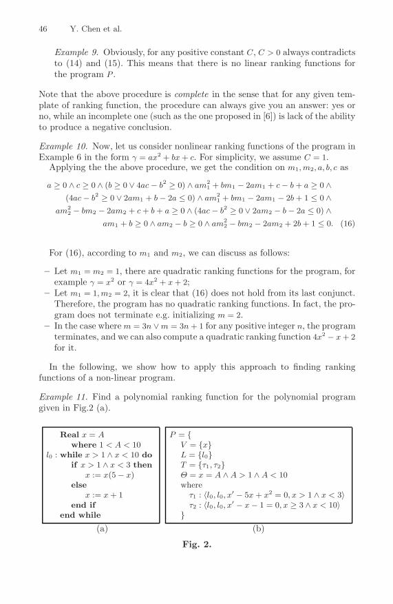
Example 11. Find a polynomial ranking function for the polynomial programgiven in Fig.2 (a).

Real x = Awhere 1 < A < 10

l0 : while x > 1 ∧ x < 10 doif x > 1 ∧ x < 3 then

x := x(5 − x)else

x := x + 1end if

end while

P = {V = {x}L = {l0}T = {τ1, τ2}Θ = x = A ∧ A > 1 ∧ A < 10where

τ1 : 〈l0, l0, x′ − 5x + x2 = 0, x > 1 ∧ x < 3〉τ2 : 〈l0, l0, x′ − x − 1 = 0, x ≥ 3 ∧ x < 10〉

}(a) (b)

Fig. 2.

Discovering Non-linear Ranking Functions 47

In order to find a ranking function of the program, we first transform theprogram to an SATS represented in Fig.2 (b). Then, assume a ranking functiontemplate with degree 1 in the form γ({x}) = ax + b.

After encoding the initial condition and then applying DISCOVERER andQEPCAD, we get a condition on a and b is

b + 10 a ≥ 0 ∧ b + a ≥ 0. (17)

Afterwards, encoding the decreasing condition w.r.t. the transition circle l0τ1→ l0

and then applying DISCOVERER and QEPCAD, we obtain

b + 4 a ≥ 0 ∧ 4 b + 25 a ≥ 0 ∧ C + 4 a ≤ 0 ∧ C + 3 a ≤ 0. (18)

Similarly, encoding the decreasing condition w.r.t. the transition circle l0τ2→ l0

and then applying DISCOVERER and QEPCAD, we get a condition

b + 11 a ≥ 0 ∧ b + 4 a ≥ 0 ∧ C + a ≤ 0. (19)

Thus, a necessary and sufficient condition on these parameters is obtained as

C > 0 ∧ a + C ≤ 0 ∧ b + 11 a ≥ 0.

So, if we assume C = 1, we can get a linear ranking function 11 − x.For this example, if we assume a ranking function template with degree 2 in

the form γ({x}) = ax2 + bx + c, and let C = 1, we get a necessary and sufficientcondition on a, b, c as

c + 10 b + 100 a ≥ 0 ∧ c + b + a ≥ 0 ∧ b + 9 a + 1 ≤ 0 ∧ b + 21 a + 1 ≤ 0 ∧(b + 2 a ≥ 0 ∨ b + 20 a ≤ 0 ∨ 4 ac − b2 ≥ 0) ∧ 16 c + 100 b + 625 a ≥ 0 ∧

c + 4 b + 16 a ≥ 0 ∧ (b + 8 a ≥ 0 ∨ 2 b + 25 a ≤ 0 ∨ 4 ac − b2 ≥ 0) ∧3 b + 15 a + 1 ≤ 0 ∧ c + 11 b + 121 a ≥ 0 ∧ c + 4 b + 16 a ≥ 0 ∧

(b + 8 a ≥ 0 ∨ b + 22 a ≤ 0 ∨ 4 ac − b2 ≥ 0) ∧ b + 7 a + 1 ≤ 0. (20)

For (20), applying PCAD in DISCOVERER we get a sample point (1, −22, 150),we therefore obtain a non-linear ranking function x2 − 22x + 150.

5 Conclusions and Future Work

This paper uses the techniques on solving semi-algebraic systems to discover non-linear ranking functions of polynomial programs. This paper also shows how touse computer algebra tools, DISCOVERER and QEPCAD, to synthesize rankingfunctions for two interesting programs.

The paper represents a part of the authors’ efforts to use DISCOVERER toverify programs. We have used it to verify reachability of linear hybrid systemsand generate symbolic termination conditions for linear programs in [27], andto discover ranking functions for polynomial programs here. Similar to Cousot’sapproach [6], DISCOVERER can also be applied to invariant generation forpolynomial programs. We will report this in another paper.

48 Y. Chen et al.

Comparing with the well-known tools REDLOG and QEPCAD, DISCOV-ERER has distinct features on solving problems related to root classification andisolation of SASs through the complete discrimination system. We will analyzeits complexity in another paper. The results of the efforts to apply DISCOV-ERER to program verification are encouraging so far, and we will continue ourefforts. The successful story of TERMINATOR [3] also encourages us to developa program verification tool based on DISCOVERER when we have sufficientexperience.

References

1. Braverman, M.: Termination of integer linear programs. In: Ball, T., Jones, R.B.(eds.) CAV 2006. LNCS, vol. 4144, pp. 372–385. Springer, Heidelberg (2006)

2. Bradley, A., Manna, Z., Sipma, H.: Terminaition of polynomial programs. In:Cousot, R. (ed.) VMCAI 2005. LNCS, vol. 3385, pp. 113–129. Springer, Heidel-berg (2005)

3. Cook, B., Podelski, A., Rybalchenko, A.: TERMINATOR: Beyond safety. In: Ball,T., Jones, R.B. (eds.) CAV 2006. LNCS, vol. 4144, pp. 415–418. Springer, Heidel-berg (2006)

4. Collins, G.E., Hong, H.: Partial cylindrical algebraic decomposition for quantifierelimination. J. of Symbolic Computation 12, 299–328 (1991)

5. Colon, M., Sipma, H.B.: Synthesis of linear ranking functions. In: Margaria, T., Yi,W. (eds.) ETAPS 2001 and TACAS 2001. LNCS, vol. 2031, pp. 67–81. Springer,Heidelberg (2001)

6. Cousot, P.: Proving program invariance and termination by parametric abstrac-tion, Langrangian Relaxation and semidefinite programming. In: Cousot, R. (ed.)VMCAI 2005. LNCS, vol. 3385, pp. 1–24. Springer, Heidelberg (2005)

7. Dams, D., Gerth, R., Grumberg, O.: A heuristic for the automatic generation ofranking functions. In: Workshop on Advances in Verification (WAVe’00), pp. 1–8(2000)

8. Dijkstra, E.W.: A Discipline of Programming. Prentice-Hall, Englewood Cliffs(1976)

9. Dolzman, A., Sturm, T.: REDLOG: Computer algebra meets computer logic. ACMSIGSAM Bulletin 31(2), 2–9

10. Floyd, R.W.: Assigning meanings to programs. In: Proc. Symphosia in AppliedMathematics, vol. 19, pp. 19–37 (1967)

11. Hoare, C.A.R.: An axiomatic basis for computer programming. Comm.ACM 12(10), 576–580 (1969)

12. Manna, Z., Pnueli, A.: Temporal Verification of Reactive Systems: Safety. Springer,Heidelberg (1995)

13. Podelski, A., Rybalchenko, A.: A complete method for the synthesis of linear rank-ing functions. In: Steffen, B., Levi, G. (eds.) VMCAI 2004. LNCS, vol. 2937, pp.239–251. Springer, Heidelberg (2004)

14. Sankaranarayanan, S., Sipma, H.B., Manna, Z.: Non-linear loop invariant genera-tion using Grobner bases. In: ACM POPL’04, pp. 318–329 (2004)

15. Tarski, A.: A Decision for Elementary Algebra and Geometry. University of Cali-fornia Press, Berkeley (1951)

16. Tiwari, A.: Termination of linear programs. In: Alur, R., Peled, D.A. (eds.) CAV2004. LNCS, vol. 3114, pp. 70–82. Springer, Heidelberg (2004)

Discovering Non-linear Ranking Functions 49

17. International Conference on Verified Software: Theories, Tools and Experiments,ETH Zurich (October 10-13, 2005)

18. Wu, W.-T.: Basic principles of mechanical theorem proving in elementary geome-tries. J. Syst. Sci. Math. 4, 207–235 (1984)

19. Xia, B., Xiao, R., Yang, L.: Solving parametric semi-algebraic systems. In: Pae,S.-i., Park, H. (eds.) ASCM 2005. Proc. the 7th Asian Symposium on ComputerMathematics, Seoul, December 8-10, pp. 8–10 (2005)

20. Xia, B., Yang, L.: An algorithm for isolating the real solutions of semi-algebraicsystems. J. Symbolic Computation 34, 461–477 (2002)

21. Xia, B., Zhang, T.: Real Solution Isolation Using Interval Arithmetic. Comput.Math. Appl. 52, 853–860 (2006)

22. Yang, L.: Recent advances on determining the number of real roots of parametricpolynomials. J. Symbolic Computation 28, 225–242 (1999)

23. Yang, L., Hou, X., Xia, B.: A complete algorithm for automated discovering of aclass of inequality-type theorems. Sci. in China (Ser. F) 44, 33–49 (2001)

24. Yang, L., Hou, X., Zeng, Z.: A complete discrimination system for polynomials.Science in China (Ser. E) 39, 628–646 (1996)

25. Yang, L., Xia, B.: Automated Deduction in Real Geometry. In: Chen, F., Wang,D. (eds.) Geometric Computation, pp. 248–298. World Scientific, Singapore (2004)

26. Yang, L., Xia, B.: Real solution classifications of a class of parametric semi-algebraic systems. In: Proc. of Int’l Conf. on Algorithmic Algebra and Logic, pp.281–289 (2005)

27. Yang, L., Zhan, N., Xia, B., Zhou, C.: Program verification by using DISCOV-ERER. In: Proc. VSTTE’05, Zurich (October 10-October 13, 2005) (to appear)