Lithium-ion Battery Modeling Using Non-equilibrium ...

Lithium-ion Battery Modeling Using

Non-equilibrium Thermodynamics

by

Todd R. Ferguson

B.S., Rensselaer Polytechnic Institute (2008)

Submitted to the Department of Chemical Engineeringin partial fulfillment of the requirements for the degree of

Doctor of Philosophy in Chemical Engineering

at the

MASSACHUSETTS INSTITUTE OF TECHNOLOGY

February 2014

c© Massachusetts Institute of Technology 2014. All rights reserved.

Author . . . . . . . . . . . . . . . . . . . . . . . . . . . . . . . . . . . . . . . . . . . . . . . . . . . . . . . . . . . . . .Department of Chemical Engineering

November 15, 2013

Certified by. . . . . . . . . . . . . . . . . . . . . . . . . . . . . . . . . . . . . . . . . . . . . . . . . . . . . . . . . .Martin Z. Bazant

ProfessorThesis Supervisor

Accepted by . . . . . . . . . . . . . . . . . . . . . . . . . . . . . . . . . . . . . . . . . . . . . . . . . . . . . . . . .Patrick S. DoyleGraduate Officer

Lithium-ion Battery Modeling Using Non-equilibrium

Thermodynamics

by

Todd R. Ferguson

Submitted to the Department of Chemical Engineeringon November 15, 2013, in partial fulfillment of the

requirements for the degree ofDoctor of Philosophy in Chemical Engineering

Abstract

The focus of this thesis work is the application of non-equilibrium thermodynamicsin lithium-ion battery modeling. As the demand for higher power and longer lastingbatteries increases, the search for materials suitable for this task continues. Tradi-tional battery modeling uses dilute solution kinetics and a fit form of the open circuitpotential to model the discharge. This work expands on this original set of equationsto include concentrated solution kinetics as well as thermodynamics-based modelingof the open circuit potential. This modification is advantageous because it does notrequire the cell to be built in order to be modeled. Additionally, this modification alsoallows phase separating materials to be modeled directly using phase field models.This is especially useful for materials such as lithium iron phosphate and graphite,which are currently modeled using a fit open circuit potential and an artificial phaseboundary (in the case of lithium iron phosphate).

This thesis work begins with a derivation of concentrated solution theory, begin-ning with a general reaction rate framework and transition state theory. This deriva-tion includes an overview of the thermodynamic definitions used in this thesis. Afterthe derivation, transport and conduction in porous media are considered. Effectivetransport properties for porous media are presented using various applicable models.Combining concentrated solution theory, mass conservation, charge conservation, andeffective porous media properties, the modified porous electrode theory equations arederived. This framework includes equations to model mass and charge conservationin the electrolyte, mass conservation in the solid intercalation particles, and electronconservation in the conducting matrix. These mass and charge conservation equa-tions are coupled to self-consistent models of the charge transfer reaction and theNernst potential. The Nernst potential is formulated using the same thermodynamicexpressions used in the mass conservation equation for the intercalation particles.The charge transfer reaction is also formulated using the same thermodynamic ex-pressions, and is presented in a form similar to the Butler-Volmer equation, whichdetermines the reaction rate based on the local overpotential. This self-consistent setof equations allows both homogeneous and phase separating intercalation materials

to be modeled.After the derivation of the set of equations, the numerical methods used to solve

the equations in this work are briefly presented, including the finite volume methodand solution methods for differential algebraic equations. Then, example simulationsat constant current are provided for homogeneous and phase separating materials todemonstrate the effect of changing the solid diffusivity and discharge rate on the cellvoltage. Other effects, such as coherency strain, are also presented to demonstratetheir effect on the behavior of particles inside the cell (e.g. suppression of phase sepa-ration). After the example simulations, specific simulations for two phase separatingmaterials are presented and compared to experiment. These simulations include slowdischarge of a lithium iron phosphate cell at constant current, and electrolyte-limiteddischarge of a graphite cell at constant potential. These two simulations are shownto agree very well with experimental data. In the last part of this thesis, the mostrecent work is presented, which is based on modeling lithium iron phosphate particlesincluding coherency strain and surface wetting. These results are qualitatively com-pared with experimental data. Finally, future work in this area is considered, alongwith a summary of the thesis.

Thesis Supervisor: Martin Z. BazantTitle: Professor

Acknowledgments

When I first joined the Bazant Group, I had very little experience with simulation

and modeling, so needless to say I was a little worried about running simulations

with complicated phase behavior. The field was very interesting to me, though, and

I was motivated to learn more about phase field modeling, simulation, and numerical

methods. I was also fortunate enough to have lots of support and guidance.

I’d first like to thank my fiancee, Danielle, and my parents for their love and

support over the past five years. Whether I was worried about presentations, papers,

or exams, they were always able to keep me grounded, and their support has helped

me through my time here at MIT. I wouldn’t have been able to do it without them.

I’d also like to thank my advisor, Martin, for his guidance and giving me direction

for my research. A large part of this thesis stems from concepts I learned in his

course, 10.626, which I was fortunate enough to TA as well. Despite his schedule

becoming increasingly busy over the past few years, he has always been able to make

time to discuss my research, whether after class or via email late at night, and this

was instrumental in my progress.

There are also a large number of post-docs, group members, and visitors I would

like to thank for their guidance. Dan Cogswell, a recent post-doc in the group,

helped me immensely with phase field modeling and numerics. His single particle

simulations have also had a large impact on my work, as can be seen throughout my

thesis. Damian Burch, who was graduating when I joined the group, helped me with

my first simulations. Peng Bai, a current post-doc in the group, has helped me to

better understand battery dynamics and experimental methods. I’d also like to thank

Michael Hess, a visitor to the group, whose discussions on graphite and lithium iron

phosphate helped me greatly. Moses Ender, who recently visited the group, helped me

with porous media modeling as well as improving my understanding of how batteries

are made. Finally, I’d like to thank Ray Smith and Edwin Sze Lun Khoo, current

group members who helped me proofread this thesis and whose discussions have

helped improve my equations and code.

Finally, this work would not have been possible without financial sponsors. I’d

like to thank NSF and MITEI for funding this research and giving me the opportunity

to research such a relevant and exciting field in energy engineering.

Contents

1 Introduction 21

1.1 Motivation . . . . . . . . . . . . . . . . . . . . . . . . . . . . . . . . . 21

1.2 Brief History of Porous Electrode Theory . . . . . . . . . . . . . . . . 23

1.3 Phase Separating Electrodes . . . . . . . . . . . . . . . . . . . . . . 26

1.3.1 Lithium Iron Phosphate . . . . . . . . . . . . . . . . . . . . 26

1.3.2 Phase-Field Models . . . . . . . . . . . . . . . . . . . . . . . 27

1.4 Thesis Outline . . . . . . . . . . . . . . . . . . . . . . . . . . . . . . . 30

2 Non-equilibrium Thermodynamics 33

2.1 Chemical Potential . . . . . . . . . . . . . . . . . . . . . . . . . . . . 33

2.2 General Theory of Reactions . . . . . . . . . . . . . . . . . . . . . . . 35

2.3 Concentrated Solution Theory . . . . . . . . . . . . . . . . . . . . . . 37

2.3.1 Diffusivity . . . . . . . . . . . . . . . . . . . . . . . . . . . . . 37

2.3.2 Derivation . . . . . . . . . . . . . . . . . . . . . . . . . . . . . 38

2.4 Conclusion . . . . . . . . . . . . . . . . . . . . . . . . . . . . . . . . . 41

3 Porous Media 43

3.1 Electrical Conductivity of the Porous Media . . . . . . . . . . . . . . 43

3.2 Conduction in Porous Media . . . . . . . . . . . . . . . . . . . . . . 47

3.3 Diffusion in Porous Media . . . . . . . . . . . . . . . . . . . . . . . 50

3.4 Conclusion . . . . . . . . . . . . . . . . . . . . . . . . . . . . . . . . . 52

4 Modified Porous Electrode Theory 55

7

4.1 Mass and Charge Conservation . . . . . . . . . . . . . . . . . . . . . 55

4.2 Faradaic Reaction Kinetics . . . . . . . . . . . . . . . . . . . . . . . . 58

4.2.1 The Nernst Equation . . . . . . . . . . . . . . . . . . . . . . . 59

4.2.2 The Modified Butler-Volmer Equation . . . . . . . . . . . . . 60

4.3 Potential Drop in the Solid Conducting Phase . . . . . . . . . . . . . 62

4.4 Diffusion in the Solid . . . . . . . . . . . . . . . . . . . . . . . . . . . 64

4.4.1 The Regular Solution Model . . . . . . . . . . . . . . . . . . . 65

4.4.2 The Cahn-Hilliard Free Energy Functional . . . . . . . . . . . 67

4.5 Non-dimensionalization and Scaling . . . . . . . . . . . . . . . . . . . 69

4.6 Conclusion . . . . . . . . . . . . . . . . . . . . . . . . . . . . . . . . . 73

5 Numerical Methods 77

5.1 The Finite Volume Method . . . . . . . . . . . . . . . . . . . . . . . 78

5.2 Differential Algebraic Equations . . . . . . . . . . . . . . . . . . . . . 81

5.3 Solving DAE’s . . . . . . . . . . . . . . . . . . . . . . . . . . . . . . . 82

5.4 DAE Formulation for Constant Current Discharge . . . . . . . . . . . 84

5.5 Conclusion . . . . . . . . . . . . . . . . . . . . . . . . . . . . . . . . . 86

6 Simulations 89

6.1 Homogeneous Particles . . . . . . . . . . . . . . . . . . . . . . . . . . 89

6.2 Phase Separating Particles . . . . . . . . . . . . . . . . . . . . . . . . 97

6.3 Conclusion . . . . . . . . . . . . . . . . . . . . . . . . . . . . . . . . . 104

7 Modeling Phase Separating Materials 107

7.1 Reaction-Limited Dynamics with Two Phases . . . . . . . . . . . . . 107

7.2 Diffusion-Limited Dynamics with Three Phases . . . . . . . . . . . . 114

7.3 Conclusion . . . . . . . . . . . . . . . . . . . . . . . . . . . . . . . . . 120

8 Modeling Lithium Iron Phosphate Electrodes 123

8.1 Single Particle Model . . . . . . . . . . . . . . . . . . . . . . . . . . . 124

8.2 Porous Electrode Modeling of Surface Wetted LFP Particles with Co-

herency Strain . . . . . . . . . . . . . . . . . . . . . . . . . . . . . . . 128

8

8.3 Simulations . . . . . . . . . . . . . . . . . . . . . . . . . . . . . . . . 130

8.3.1 Comparison to LFP Electrodes on Charge and Discharge . . . 135

8.4 Comparison with LFP Discharge Curves . . . . . . . . . . . . . . . . 142

8.5 Conclusion . . . . . . . . . . . . . . . . . . . . . . . . . . . . . . . . . 143

9 Conclusion 145

9

List of Figures

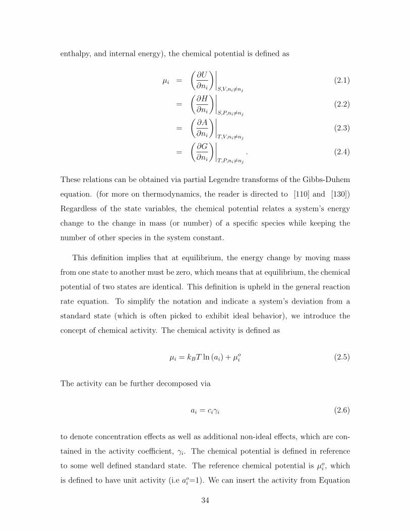
2-1 Typical reaction energy landscape. The set of atoms involved in

the reaction travels through a transition state as it passes from one

state to the other in a landscape of total excess chemical potential as

a function of the atomic coordinates. . . . . . . . . . . . . . . . . . . 36

2-2 Typical diffusion energy landscape. The same principles for reac-

tions can also be applied to solid diffusion, where the diffusing molecule

explores a landscape of excess chemical potential, hopping by thermal

activation between nearly equivalent local minima. . . . . . . . . . . 38

2-3 Lattice gas model for diffusion. The atoms are assigned a constant

excluded volume by occupying sites on a grid. Atoms can only jump

to an open space, and the transition state (red dashed circle) requires

two empty spaces. . . . . . . . . . . . . . . . . . . . . . . . . . . . . . 39

2-4 Diffusion through a solid. The flux is given by the reaction rate

across the area of the cell, Acell. In this lattice model, atoms move

between available sites. . . . . . . . . . . . . . . . . . . . . . . . . . . 40

3-1 Wiener bounds on the effective conductivity of a two-phase

anisotropic material. The left figure demonstrates the upper con-

ductivity limit achieved by stripes aligned with the field, which act like

resistors in parallel. The right figure demonstrates the lower bound

with the materials arranged in transverse stripes to act like resistors

in series. . . . . . . . . . . . . . . . . . . . . . . . . . . . . . . . . . 44

11

3-2 Hashin-Shtrikman bounds on the effective conductivity of a

two-phase isotropic material. Isotropic random composite of space-

filling coated spheres which attain the bounds. The white represents

material with conductivity σ1 and the black represents material with

conductivity σ2. Maximum conductivity is achieved when σ1 > σ2 and

minimum conductivity is obtained when σ2 > σ1. The volume fractions

Φ1 and Φ2 are the same. . . . . . . . . . . . . . . . . . . . . . . . . . 45

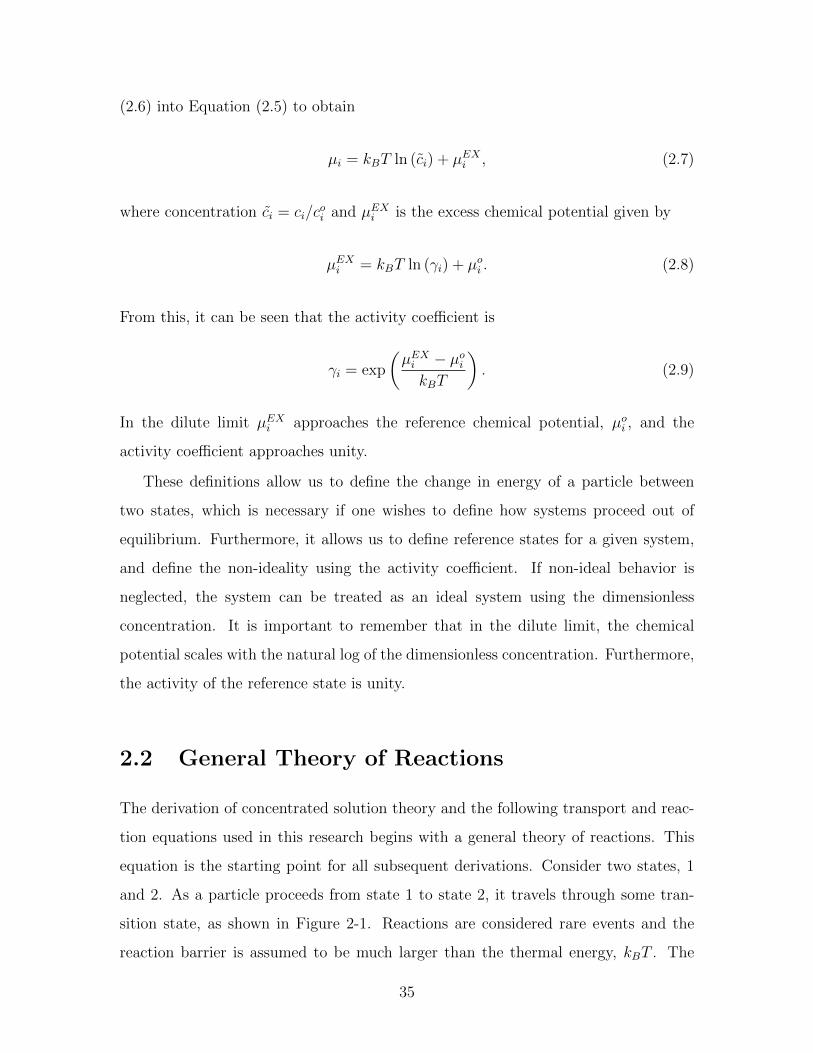
3-3 Conductivity bounds for two-phase composites versus vol-

ume fraction. The above figure shows the Wiener bounds (blue) for

an anisotropic two component material and Hashin-Shtrikman bounds

(red) for an isotropic two component material versus the volume frac-

tion of material 1. The conductivities used to produce the figure are

σ1 = 1 and σ2 = 0.1. . . . . . . . . . . . . . . . . . . . . . . . . . . . 46

3-4 Example of a porous volume. This is an example of a typical porous

volume. A mixture of solid particles is permeated by an electrolyte.

The porosity, εp, is the volume of electrolyte as a fraction of the volume

of the cube. . . . . . . . . . . . . . . . . . . . . . . . . . . . . . . . . 47

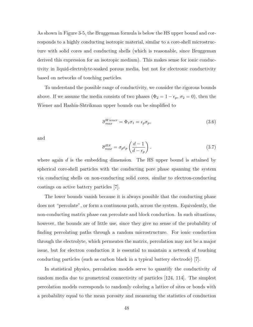
3-5 Various models for effective conductivity in 3D. This figure

demonstrates the effective conductivity (scaled by the pore conduc-

tivity) using Wiener bounds, Hashin-Shtrikman bounds, a percolation

model, and the Bruggeman formula. The percolation model uses a

critical porosity of εc = 0.25. . . . . . . . . . . . . . . . . . . . . . . . 49

3-6 Tortuosity versus porosity for different effective conductivity

models. This plot gives the tortuosity for different porosity values.

While the Wiener and Hashin-Shtrikman models produce finite tor-

tuosities, the percolation and Bruggeman models diverge as porosity

goes to zero. . . . . . . . . . . . . . . . . . . . . . . . . . . . . . . . . 53

12

4-1 Regular solution model for the free energy of a homogeneous

mixture. This figure shows the effect of the regular solution parameter

Ω (mean pair interaction energy) and temperature T on the free energy

versus filling fraction c of a regular solution of atoms and vacancies on

a lattice. For Ω < 2kBT , there is a single minimum. For Ω > 2kBT ,

there are two minima. This produces phase separation, as the system is

unstable with respect to infinitesimal perturbations near the spinodal

concentration, which is where the curvature of the free energy changes. 66

6-1 Plot axes for diffusion-limited solid-solution particles. This fig-

ure shows how the simulation results below are plotted for porous elec-

trodes with isotropic solid solution particles. The y-axis of the contour

plots represent the depth of the particles while the x-axis represents

the depth into the electrode. The particles are modeled in 1D. . . . . 90

6-2 Effect of current on homogeneous particles. This figure demon-

strates the effect of different discharge rates on the voltage profile. The

non-dimensional currents correspond to roughly C/3, 3C, and 15C. The

solid diffusion is fast, with δd = 1. . . . . . . . . . . . . . . . . . . . . 92

6-3 Depletion of the electrolyte at higher current. This figure shows

the depletion of the electrolyte accompanying Figure 6-2 for the 15C

discharge. The left figure shows the solid concentration while the right

figure demonstrates the electrolyte concentration profile in the separa-

tor and electrode. . . . . . . . . . . . . . . . . . . . . . . . . . . . . . 93

6-4 Effect of current on homogeneous particles with slower solid

diffusion. This figure demonstrates the effect of different discharge

rates on the voltage profile. The non-dimensional currents correspond

to roughly C/3, 3C, and 15C. The solid diffusion is slower than the

electrolyte diffusion (δd = 100). . . . . . . . . . . . . . . . . . . . . . 95

13

6-5 Effect of solid diffusivity on homogeneous particles. This figure

demonstrates the effect of decreasing solid diffusivity on the voltage

profile. Each of these simulations was run at a dimensionless exchange

current density of 0.01 and a dimensionless current of 0.01. . . . . . . 96

6-6 Plot axes for reaction-limited phase separating particles. This

figure shows how the results are plotted below for porous electrodes

with reaction-limited phase separating nanoparticles. The y-axis of

the contour plots represent the length along the surface of the particle,

since diffusion is assumed to be fast in the depth direction. The x-axis

represents the depth in the electrode. . . . . . . . . . . . . . . . . . . 98

6-7 Phase separating particles slowly discharged. This figure shows

slow discharge (approx. C/30) of phase separating particles. Adequate

electrolyte diffusion and discrete filling don’t allow time for the parti-

cles to phase separate early on. At the end of the discharge, sufficient

time allows the particles to phase separate. . . . . . . . . . . . . . . . 99

6-8 Phase separating particles including coherent stress effects

slowly discharged. This figure shows slowly discharge (approx. C/30)

phase separating particles. The inclusion of the coherent stress effects

suppresses phase separation inside the particles. This figure is the same

as Figure 6-7, with an additional coherent stress term. . . . . . . . . 101

6-9 Effect of current on phase separating particles. When discharged

at a higher C-rate (in this example, 3C), the size of the discrete particle

filling is larger, leading to more particles filling simultaneously and a

voltage curve that resembles solid solution behavior. . . . . . . . . . . 103

6-10 Equivalent circuit model for a porous electrode. This equivalent

circuit represents a typical porous electrode in cases without significant

electrolyte depletion, where the pore phase maintains nearly uniform

conductivity. Resistors represent the contact, transport, and charge

transfer resistances, and the capacitance of the particles is represented

by a capacitor. All elements are not necessarily linear. . . . . . . . . 104

14

7-1 Voltage half gap and effective regular solution. Figure a denotes

the voltage half gap on discharge from Cogswell and Bazant and the

resulting effective regular solution parameter as a function of the wet-

ted area to volume ratio. Figure b demonstrates various effective open

circuit potential profiles for different sized particles. . . . . . . . . . . 110

7-2 Voltage gap fit to data. This figure shows the fit of the model

to experimental data from Dreyer et al. [54] Figure (a) shows an

overlay of the simulation with the data for C/1000, C/200, and C/131.

Figure (b) shows the effect of particle size variance on the voltage

curve. Figure (c) compares the voltage gap to data with the additional

C/100 and C/50 rates. Also the voltage gap with no size effect is

demonstrated. The inlay shows the particle size distribution used to

fit the data. Figure (d) shows representative particle sizes for the

variances given in figure (b) at a filling fraction of 0.5. Experimental

data in figures (a-c) from [54], provided courtesy of Miran Gaberscek 112

7-3 Comparison of graphite model to OCP and the electrolyte dif-

fusion limited case Figure (a) shows a comparison of the graphite

model with the OCP (data from [101]). Figure (b) is a contour plot of

the free energy given by the model. The free energy surface has four

minima near the corners. As lithium intercalates, the reaction coor-

dinate proceeds along the lines connecting these minima. Figure (c)

shows the red/gold interface position versus time compared to exper-

imental data. Figure (d) shows a comparison between experimental

data (from video of the experiment) and simulation. Experimental

data in figures (c) and (d) is adapted from [67]. . . . . . . . . . . . 118

8-1 Slow discharge of different sized particles This plot shows the

voltage profile for slow discharge of different sized particles. The

shrinking of the voltage overshoot required to drive lithiation can be

seen as particle size is decreased. . . . . . . . . . . . . . . . . . . . . 126

15

8-2 Different schemes for addressing particle size distributions

The figure denotes two possible methods to include particle size distri-

butions. The scheme on the left uses a 2D grid with one particle size

in each volume while the scheme on the right uses a 1D grid with a

particle size distribution inside each volume. For fewer discretizations,

the scheme on the right captures the active area better than the scheme

on the left. . . . . . . . . . . . . . . . . . . . . . . . . . . . . . . . . . 129

8-3 C/50 discharge of ACR MPET model This figure shows solid

concentration profiles and a voltage versus filling fraction for C/50

discharge. The red and blue dots correspond to the colored solid con-

centration profiles. . . . . . . . . . . . . . . . . . . . . . . . . . . . . 131

8-4 1.5C discharge of ACR MPET model This figure shows solid

concentration profiles and a voltage versus filling fraction for 1.5C dis-

charge. The red and blue dots correspond to the colored solid concen-

tration profiles. . . . . . . . . . . . . . . . . . . . . . . . . . . . . . . 132

8-5 5C discharge of ACR MPET model This figure shows solid con-

centration profiles and a voltage versus filling fraction for 5C discharge.

The red and blue dots correspond to the colored solid concentration

profiles. . . . . . . . . . . . . . . . . . . . . . . . . . . . . . . . . . . 133

8-6 C/50 charge of ACR MPET model This figure shows solid con-

centration profiles and a voltage versus filling fraction for C/50 charge.


profiles. . . . . . . . . . . . . . . . . . . . . . . . . . . . . . . . . . . 134

8-7 1.5C charge of ACR MPET model This figure shows solid con-

centration profiles and a voltage versus filling fraction for 1.5C charge.


profiles. . . . . . . . . . . . . . . . . . . . . . . . . . . . . . . . . . . 135

16

8-8 Electrode after discharge This figure shows the TEM and X-ray

absorption spectroscopy images for discharge rates of (a) C/50 (b)

1.5C and (c) 5C. The circles indicate the positions of “mixed” particles

which are either homogeneous or a mixture of full and empty portions,

denoted by the yellow color. Figure courtesy of Li and Chueh. [91] . 136

8-9 Electrode after 1.5C charge This figure shows the TEM and X-ray

absorption spectroscopy images for a 1.5C charging rate. The circles

indicate the positions of “mixed” particles which are either homoge-

neous or a mixture of full and empty portions, denoted by the yellow

color. Figure courtesy of Li and Chueh. [91] . . . . . . . . . . . . . . 137

8-10 Relaxation after 1.5 discharge of ACR MPET model This fig-

ure shows solid concentration profiles and a voltage versus time for

relaxation after a 1.5C discharge. The red and blue dots correspond

to the colored solid concentration profiles at the beginning and end of

the relaxation. . . . . . . . . . . . . . . . . . . . . . . . . . . . . . . . 138

8-11 Relaxation after 5C discharge of ACR MPET model This fig-

ure shows solid concentration profiles and a voltage versus time for

relaxation after a 5C discharge. The red and blue dots correspond to

the colored solid concentration profiles at the beginning and end of the

relaxation. . . . . . . . . . . . . . . . . . . . . . . . . . . . . . . . . . 139

8-12 Relaxation after 1.5C charge of ACR MPET model This figure

shows solid concentration profiles and a voltage versus time for relax-

ation after a 1.5C charge. The red and blue dots correspond to the

colored solid concentration profiles at the beginning and end of the

relaxation. . . . . . . . . . . . . . . . . . . . . . . . . . . . . . . . . . 141

17

8-13 Comparison of ACR MPET model with electronic effects to

discharge curves Figure (a) shows the fit to the 1C charge and dis-

charge curves. Using the same parameters, figure (b) shows simulations

at C/40, 1C, 2C, 3C, 4C, and 5C compared to experimental data. Fig-

ures provided courtesy of Moses Ender. The fit was performed using

the MPET model presented in this chapter including electron conduc-

tion in the solid matrix. . . . . . . . . . . . . . . . . . . . . . . . . . 142

18

List of Tables

4.1 Dimensional set of equations. A list of the set of dimensional equa-

tions for Modified Porous Electrode Theory. The boundary conditions

listed here are for constant current discharge. . . . . . . . . . . . . . . 74

5.1 BDF coefficients This table lists the BDF coefficients, for up to sixth

order (k is the order). This table is adapted from [4]. . . . . . . . . . 83

19

Chapter 1

Introduction

Modeling is a key component of any design process. An accurate model allows one

to interpret experimental data, identify rate limiting steps and predict system be-

havior, while providing a deeper understanding of the underlying physical processes.

In systems engineering, empirical models with fitted parameters are often used for

design and control, but it is preferable, whenever possible, to employ models based on

microscopic physical or geometrical parameters, which can be more easily interpreted

and optimized.

1.1 Motivation

In the case of electrochemical energy storage devices, such as batteries, fuel cells,

and supercapacitors, the systems approach is illustrated by equivalent circuit mod-

els, which are widely used in conjunction with impedance spectroscopy to fit and

predict cell performance and degradation. This approach is limited, however, by the

difficulty in unambiguously interpreting fitted circuit elements and in making predic-

tions for the nonlinear response to large operating currents. There is growing interest,

therefore, in developing physics-based porous electrode models and applying them for

battery optimization and control [111]. Quantum mechanical computational meth-

ods have demonstrated the possibility of predicting bulk material properties, such

as open circuit potential and solid diffusivity, from first principles [40], but coarse-

21

grained continuum models are needed to describe the many length and time scales of

interfacial reactions and multiphase, multicomponent transport phenomena.

Mathematical models could play a crucial role in guiding the development of new

intercalation materials, electrode microstructures, and battery architectures, in order

to meet the competing demands in power density and energy density for different

envisioned applications, such as electric vehicles or renewable (e.g. solar, wind) energy

storage. Porous electrode theory, pioneered by J. Newman and collaborators, provides

the standard modeling framework for battery simulations today [98]. As reviewed in

the next section, this approach has been developed for over half a century and applied

successfully to many battery systems. The treatment of the active material, however,

remains rather simple, and numerous parameters are often needed to fit experimental

data.

In porous electrode theory for Li-ion batteries, transport is modeled via volume av-

eraged conservation equations [50]. The solid active particles are modeled as spheres,

where intercalated lithium undergoes isotropic linear diffusion [51, 52]. For phase

separating materials, such as LixFePO4 (LFP), each particle is assumed to have a

spherical phase boundary that moves as a “shrinking core”, as one phase displaces

the other [123, 46, 132]. In these models, the local Nernst equilibrium potential is

fitted to the global open circuit voltage of the cell, but this neglects non-uniform

composition, which makes the voltage plateau an emergent property of the porous

electrode [54, 53, 8, 45]. For thermodynamic consistency, all of these phenomena

should derive from common thermodynamic principles and cannot be independently

fitted to experimental data. The open circuit voltage reflects the activity of interca-

lated ions, which in turn affects ion transport in the solid phase and Faradaic reactions

involving ions in the electrolyte phase [12, 13].

In this thesis, porous electrode theory is extended to non-ideal active materials,

including those capable of phase transformations. The starting point is a general

phase-field theory of ion intercalation kinetics developed by the Bazant group over

the past five years [13, 120, 33, 16, 32, 8], which has recently led to a quantitative

understanding of phase separation dynamics in LFP nanoparticles [45, 44]. The ionic

22

fluxes in all phases are related to electrochemical potential gradients, consistent with

non-equilibrium thermodynamics [62, 10]. This approach has been used extensively

in recent years to model transport in electrochemical systems [74, 88, 87, 90, 89, 21,

79, 80, 102, 17] and nonlinear electrokinetic phenomena [16, 15, 20, 126]. For ther-

modynamic consistency, we also relate the Faradaic reaction rate to electrochemical

potential differences between the oxidized, reduced, and transition states, leading to

a generalized Butler-Volmer equation [13, 8, 45] suitable for phase-separating mate-

rials. These elements are integrated in a general porous electrode theory, where the

active material can be described by a Cahn-Hilliard phase-field model [10, 97], as in

nanoscale simulations of Li-ion battery materials [66, 61, 120, 33, 32, 128, 76, 8, 45].

This allows us to describe the non-equilibrium thermodynamics of porous battery

electrodes in terms of well established physical principles for ion intercalation in

nanoparticles.

1.2 Brief History of Porous Electrode Theory

We begin by reviewing volume-averaged porous electrode theory, which has been the

standard approach in battery modeling for the past 50 years. The earliest papers deal-

ing with porous electrode theory were published in the late 1950’s and early 1960’s,

by Ksenzhek and Stender [83, 84, 85] and Euler and Nonnenmacher [57]. This work

treated current density distributions in porous electrodes, which were characterized

by volume averaged properties, such as porosity, average surface area per volume,

and conductivity.

A few years later, Newman and Tobias expanded the analysis to account for

the effects of concentration variations on kinetics with concentration independent

electrolyte properties. [100] This paper also introduced the well known equation for

mass conservation inside a porous electrode undergoing reactions. Around the same

time, de Levie published his work modeling diffusion inside pores, capacitance effects,

and combined effects of double layer capacitance, diffusion, and kinetics. [47, 48]

These models included linear capacitance effects for the double layer and utilized

23

equivalent circuit models for the porous electrode.

Another notable paper is by Ksenzhek, which incorporated concentrated solution

theory in the transport equations inside a porous electrode, and referred to gradients

in electrochemical potential as the driving force for transport. [82] (for more on

force and flux coupling, refer to [10]) Ksenzhek’s paper introduced many of the same

concepts used in this paper to treat transport processes in the electrode. Much of the

earlier work on modeling porous electrodes relied on deriving the volume averaged

governing equations as well as some analytical results for small overpotential (i.e.

linearized) or high overpotential (i.e. Tafel) regime kinetics. [72] Other notable

papers include modeling transport effects in steady state operation [63] and transient

behavior of a porous electrode subjected to galvanostatic discharge with sinusoidal

perturbations. [112]

Many of the volume averaged principles have underlying assumptions regarding

properties of the cell that can be critical to performance. The validity of these as-

sumptions was reviewed by Grens. [71] It was found that the assumption of constant

conductivity can be used over a wide range of operating conditions. The assumption

of constant electrolyte concentration, which was used to simplify systems in early

papers, is only valid over a narrow range of operating conditions, as is expected.

In 1975, Newman and Tiedemann published a review of porous electrode the-

ory. [99] This paper summarized mass and charge conservation equations and kinetic

equations for batteries and other types of electrochemical systems. A few years later,

Atlung et al. investigated the dynamics of solid solution (i.e. intercalation) electrodes

for different time scales with respect to the limiting current. [6] Pollard and New-

man investigated the transient behavior of porous electrodes at high exchange current

densities (i.e. small overpotential). [107] These two papers appear to be some of the

earliest studies of the time dependence of porous electrode systems. Up to this point,

the literature was predominantly based on linearized Butler-Volmer and exponential

Tafel kinetics, due to limited computational power.

As computers and numerical methods advanced, so did simulations of porous

electrodes. West et al. demonstrated the use of numerical methods to simulate

24

discharge of a porous TiS2 electrode (without the separator), and how the main

limiting factor is the depletion of the electrolyte. [138] This is one of the earliest

demonstrations of solving the porous electrode equations using numerical methods.

About ten years later, Doyle, Fuller and Newman modeled a separator and porous

electrode under constant current discharge. [51] This paper was one of the first

to model the reaction rate with the Butler-Volmer equation, instead of linearized

kinetics or a Tafel equation. The next year, Fuller, Doyle and Newman published a

similar model of a dual lithium-ion insertion cell (graphite anode and manganese oxide

cathode) [59]. Doyle et al. then published a comparison of model predictions with

experimental data for the full lithium-ion battery (anode and cathode) [52] These

papers are of great importance in the field, as they developed the first complete

simulations of lithium-ion batteries and solidified the role of porous electrode theory

in modeling these systems. The same theoretical framework has been applied to many

other types of cells, such as lithium-sulfur [86] and LFP [123, 46] batteries. This

framework has also been applied to lithium polymer batteries, for which Arora et al.

have demonstrated good agreement with experimental data for high-rate discharge.

[3]

Battery models invariably assume electroneutrality, but diffuse charge in porous

electrodes has received increasing attention over the past decade, driven by applica-

tions in energy storage and desalination. The effects of double-layer capacitance in a

porous electrode were originally considered using only linearized low-voltage models

[75, 134], which are equivalent to transmission line circuits [47, 48, 55]. Recently, the

full nonlinear dynamics of capacitive charging and salt depletion have been analyzed

and simulated in both flat [18, 102] and porous [22] electrodes. The combined effects of

electrostatic capacitance and pseudo-capacitance due to Faradaic reactions have also

been incorporated in porous electrode theory [23, 24], using Frumkin-Butler-Volmer

kinetics [19, 14, 29, 81, 73]. These models have been successfully used to predict the

nonlinear dynamics of capacitive desalination by porous carbon electrodes [25, 109].

Computational and experimental advances have also been made to study porous

electrodes at the microstructural level and thus test the formal volume-averaging,

25

which underlies macroscopic continuum models. Garcia et al. performed finite-

element simulations of ion transport in typical porous microstructures for Li-ion

batteries [61], and Garcia and Chang simulated hypothetical inter-penetrating 3D

battery architectures at the particle level [60]. Recently, Smith, Garcia and Horn

analyzed the effects of microstructure on battery performance for various sizes and

shapes of particles in a Li1−xC6/LixCoO2 cell [122]. The study used 3D image recon-

struction of a real battery microstructure by focused ion beam milling, which has led

to detailed studies of microstructural effects in porous electrodes [133, 131, 78]. In this

paper, we will discuss mathematical bounds on effective diffusivities in porous media,

which could be compared to results for actual battery microstructures. Recently, it

has also become possible to observe lithium ion transport at the scale in individual

particles in porous Li-ion battery electrodes [9, 137], which could be invaluable in

testing the dynamical predictions of new mathematical models.

1.3 Phase Separating Electrodes

1.3.1 Lithium Iron Phosphate

The discovery of LFP as a cathode material by the Goodenough group in 1997 has had

a large and unexpected impact on the battery field, which provides the motivation

for our work. LFP was first thought to be a low-power material, and it demonstrated

poor capacity at room temperature. [104] The capacity has since been improved via

conductive coatings and the formation of nanoparticles. [113, 69], and the rate ca-

pability has been improved in similar ways [68, 92]. With high carbon loading to

circumvent electronic conductivity limitations, LFP nanoparticles can now be dis-

charged in 10 seconds [76]. Off-stoichiometric phosphate glass coatings contribute to

this high rate, not only in LFP, but also in LiCoO2 [127].

It has been known since its discovery that LFP is a phase separating material, as

evidenced by a flat voltage plateau in the open circuit voltage [104, 129]. There are

a wide variety of battery materials with multiple stable phases at different states of

26

charge [70], but LixFePO4 has a particularly strong tendency for phase separation,

with a miscibility gap (voltage plateau) spanning across most of the range from x = 0

to x = 1 at room temperature. Padhi et al. first depicted phase separation inside LFP

particles schematically as a “shrinking core” of one phase being replaced by an outer

shell of the other phase during charge/discharge cycles [104]. Srinivasan and Newman

encoded this concept in a porous electrode theory of the LFP cathode with spherical

active particles, containing spherical shrinking cores. [123] Recently, Dargaville and

Farrell have expanded this approach to predict active material utilization in LFP

electrodes. [46] Thorat et al. have also used the model to gain insight into rate-

limiting mechanisms inside LFP cathodes. [132]

To date, the shrinking-core porous electrode model is the only model to success-

fully fit the galvanostatic discharge of an LFP electrode, but the results are not

fully satisfactory. Besides neglecting the microscopic physics of phase separation, the

model relies on fitting a concentration-dependent solid diffusivity, whose inferred val-

ues are orders of magnitude smaller than ab initio simulations [96, 92] or impedance

measurements [105]. More consistent values of the solid diffusivity have since been

obtained by different models attempting to account for anisotropic phase separation

with elastic coherency strain. [139] Most troubling for the shrinking core picture, how-

ever, is the direct observation of phase boundaries with very different orientations. In

2006, Chen, Song, and Richardson published images showing the orientation of the

phase interface aligned with iron phosphate planes and reaching the active facet of the

particle. [41] This observation was supported by experiments of Delmas et al., who

suggested a “domino-cascade model” for the intercalation process inside LFP [49].

With further experimental evidence for anisotropic phase morphologies [103, 137],

it has become clear that a new approach is needed to capture the non-equilibrium

thermodynamics of this material.

1.3.2 Phase-Field Models

Phase-field models are widely used to describe phase transformations and microstruc-

tural evolution in materials science [10, 42], but they are relatively new to electro-

27

chemistry. In 2004, Guyer, Boettinger, Warren and McFadden [64, 65] first mod-

eled the sharp electrode/electrolyte interface with a continuous phase field varying

between stable values 0 and 1, representing the liquid electrolyte and solid metal

phases. As in phase-field models of dendritic solidification [77, 27, 26, 28], they used

a simple quartic function to model a double-welled homogeneous free energy. They

described the kinetics of electrodeposition [65] (converting ions in the electrolyte to

solid metal) by Allen-Cahn-type kinetics [2, 42], linear in the thermodynamic driv-

ing force, but did not make connections with the Butler-Volmer equation. Several

groups have used this approach to model dendritic electrodeposition and related pro-

cesses [5, 118, 108]. Also in 2004, Han, Van der Ven and Ceder [66] first applied the

Cahn-Hilliard equation[34, 35, 39, 36, 10, 42] to the diffusion of intercalated lithium

ions in LFP, albeit without modeling reaction kinetics.

Building on these advances, Bazant developed a general theory of charge-transfer

and Faradaic reaction kinetics in concentrated solutions and solids based on non-

equilibrium thermodynamics [13, 11, 12], suitable for use with phase-field models. The

exponential Tafel dependence of the current on the overpotential, defined in terms

of the variational chemical potentials, was first reported in 2007 by Singh, Ceder

and Bazant [120, 119], but with spurious pre-factor, corrected by Burch [31, 32].

The model was used to predict “intercalation waves” in small, reaction-limited LFP

nanoparticles in 1D [120], 2D [33], and 3D [128], thus providing a mathematical

description of the domino cascade phenomenon [49]. The complete electrochemical

phase-field theory, combining the Cahn-Hilliard with Butler-Volmer kinetics and the

cell voltage, appeared in 2009 lectures notes [11, 12] and was applied to LFP nanopar-

ticles [8, 45].

The new theory has led to a quantitative understanding of intercalation dynamics

in single nanoparticles of LFP. Bai, Cogswell and Bazant [8] generalized the Butler-

Volmer equation using variational chemical potentials (as derived in the supporting

information) and used it to develop a mathematical theory of the suppression of phase

separation in LFP nanoparticles with increasing current. This phenomenon, which

helps to explain the remarkable performance of nano-LFP, was also suggested by Malik

28

and Ceder based on bulk free energy calculations [93], but the theory shows that it is

entirely controlled by Faradaic reactions at the particle surface [8, 45]. Cogswell and

Bazant [45] have shown that including elastic coherency strain in the model leads to

a quantitative theory of phase morphology and lithium solubility. Experimental data

for different particles sizes and temperatures can be fitted with only two parameters

(the gradient penalty and regular solution parameter, defined below).

The goal of the present work is to combine the phase-field theory of ion interca-

lation in nanoparticles with classical porous electrode theory to arrive at a general

mathematical framework for non-equilibrium thermodynamics of porous electrodes.

Our work was first presented at the Fall Meeting of the Materials Research Society in

2010 and again at the Electrochemical Society Meetings in Montreal and Boston in

2011. Around the same time, Lai and Ciucci were thinking along similar lines [87, 89]

and published an important reformulation of Newman’s porous electrode theory based

non-equilibrium thermodynamics [90], but they did not make any connections with

phase-field models or phase transformations at the macroscopic electrode scale. (Their

treatment of reactions also differs from Bazant’s theory of generalized Butler-Volmer

or Marcus kinetics [13, 12, 11].)

In this thesis, a variational thermodynamic description of electrolyte transport,

electron transport, electrochemical kinetics, and phase separation is developed and

applied to Li-ion batteries in what appears to be the first mathematical theory and

computer simulations of macroscopic phase transformations in porous electrodes. Sim-

ulations of discharge into a cathode consisting of multiple phase-separating particles

interacting via an electrolyte reservoir at constant chemical potential were reported

by Burch [31], who observed “mosaic instabilities”, where particles transform one-

by-one at low current. This phenomenon was elegantly described by Dreyer et al.

in terms of a (theoretical and experimental) balloon model, which helps to explain

the noisy voltage plateau and zero-current voltage gap in slow charge/discharge cy-

cles of porous LFP electrodes [54, 53]. These studies, however, did not account for

electrolyte transport and associated macroscopic gradients in porous electrodes under-

going phase transformations, which are the subject of this work. To do this, we must

29

reformulate Faradaic reaction kinetics for concentrated solutions, consistent with the

Cahn-Hilliard equation for ion intercalation and Newman’s porous electrode theory

for the electrolyte.

This thesis also presents fitting of the voltage gap data data presented by Dreyer

et al.. [54] A pseudocapacitor model with a voltage gap fit to the work of Cogswell

and Bazant [44] is used to fit a particle size distribution and contact resistance

and demonstrate why different experiments observe different values of the voltage

gap, and why the observed voltage gap does not match the voltage gap predicted by

thermodynamics alone.

Additionally, a model for the free energy of graphite is presented and fit to data for

the case of electrolyte transport limited potentiostatic discharge. This new graphite

free energy model captures three phase behavior of lithiated graphite (i.e. empty,

half full, and full states) by using two representative graphite layers along with an

interaction energy and what can be thought of as a strain energy. Although graphite

actually has more than three phases [101], for the purpose of this simulation (i.e.

matching to experimental data) three phases are sufficient. The data the simulations

are fit to determines the concentration of lithium in graphite using the color change

associated with lithiation, and only three colors are presented, corresponding to the

three phases (i.e. empty, half, and full).

Building on the recent work of Cogswell and Bazant [44], surface wetted LiFePO4

particles inside a porous electrode with approximated coherency strain are also pre-

sented in this thesis. These simulations are compared qualitatively to experimental

data from Li and Chueh. [43] Finally, a simulation including electron conduction

with the aforementioned surface wetted LiFePO4 particles and coherency strain is

compared to experimental data.

1.4 Thesis Outline

This thesis will begin with a brief overview of the thermodynamics used as well as

a derivation of concentrated solution theory that will be used throughout the rest of

30

the chapters. This overview is followed by the derivation of the full set of modified

porous electrode theory equations, as well as the non-dimensionalization that is used

in later simulations. Additional examples demonstrating the use of the Cahn-Hilliard

free energy functional are also included.

After the derivation of the full set of equations, some numerical methods are briefly

discussed. The focus of this thesis work is on the model development itself. The

chapter on numerics is not intended to be a full review of all methods available, but

to present some potential methods that can be used as well as how the equations were

formulated and discretized for the simulations in this thesis work. After the chapter

on numerics, some example simulations from the first publication as a result of this

work are presented. The purpose of these simulations is to demonstrate the effect of

changing parameters in the model, namely the discharge rate (i.e. the current) and

solid diffusivity.

After the general simulation results, more specific results along with a comparison

to data will be presented. The first data set analyzed is that of Dreyer et al.. [53]

Using a “pseudocapacitor” model, which assumes all solid particles are homogeneous,

a particle size distribution and contact resistance are fit to the voltage gap. The size

distribution is based on simulations from Cogswell and Bazant. [44] Then, a new

graphite free energy model is used to fit the experimental data of Harris et al. [67]

using an electrolyte diffusion limited cell.

The second to last chapters of this thesis represents the most recent work. It

includes simulations using the surface wetted LiFePO4 particles with coherency strain

from Cogswell and Bazant [44] inside a porous electrode. The results are qualitatively

compared to recent experimental data from Li and Chueh (similar to previous work

by Chueh et al. [43]). The final section considers the surface wetted particles with

bulk electronic conduction effects and compares this to data from Ender. [56] The

final chapter is a summary of the work presented in this thesis as well as future work.

31

Chapter 2

Non-equilibrium Thermodynamics

Classical thermodynamics deals with equilibrium states. However, time evolution is

a non-equilibrium process. Non-equilibrium thermodynamics allows the evolution of

energy states to be modeled using thermodynamic models. The underlying assump-

tion is that the system proceeds through small perturbations from equilibrium, such

that changes can be linearized. More specifically, this requires that processes are

reversible, which implies that entropy is conserved.

2.1 Chemical Potential

Chemical potential is the change in energy associated with the change in mass of

a system. It is an additional term in the energy equations which accounts for the

inherent energy particles bring as they are added or removed form the system. The

chemical potential has a different definition based on the state variables of the system.

For the four different types of energy (Gibbs free energy, Helmholtz free energy,

33

enthalpy, and internal energy), the chemical potential is defined as

µi =

(∂U

∂ni

)∣∣∣∣S,V,ni 6=nj

(2.1)

=

(∂H

∂ni

)∣∣∣∣S,P,ni 6=nj

(2.2)

=

(∂A

∂ni

)∣∣∣∣T,V,ni 6=nj

(2.3)

=

(∂G

∂ni

)∣∣∣∣T,P,ni 6=nj

. (2.4)

These relations can be obtained via partial Legendre transforms of the Gibbs-Duhem

equation. (for more on thermodynamics, the reader is directed to [110] and [130])

Regardless of the state variables, the chemical potential relates a system’s energy

change to the change in mass (or number) of a specific species while keeping the

number of other species in the system constant.

This definition implies that at equilibrium, the energy change by moving mass

from one state to another must be zero, which means that at equilibrium, the chemical

potential of two states are identical. This definition is upheld in the general reaction

rate equation. To simplify the notation and indicate a system’s deviation from a

standard state (which is often picked to exhibit ideal behavior), we introduce the

concept of chemical activity. The chemical activity is defined as

µi = kBT ln (ai) + µoi (2.5)

The activity can be further decomposed via

ai = ciγi (2.6)

to denote concentration effects as well as additional non-ideal effects, which are con-

tained in the activity coefficient, γi. The chemical potential is defined in reference

to some well defined standard state. The reference chemical potential is µoi , which

is defined to have unit activity (i.e aoi=1). We can insert the activity from Equation

34

(2.6) into Equation (2.5) to obtain

µi = kBT ln (ci) + µEXi , (2.7)

where concentration ci = ci/coi and µEXi is the excess chemical potential given by

µEXi = kBT ln (γi) + µoi . (2.8)

From this, it can be seen that the activity coefficient is

γi = exp

(µEXi − µoikBT

). (2.9)

In the dilute limit µEXi approaches the reference chemical potential, µoi , and the

activity coefficient approaches unity.

These definitions allow us to define the change in energy of a particle between

two states, which is necessary if one wishes to define how systems proceed out of

equilibrium. Furthermore, it allows us to define reference states for a given system,

and define the non-ideality using the activity coefficient. If non-ideal behavior is

neglected, the system can be treated as an ideal system using the dimensionless

concentration. It is important to remember that in the dilute limit, the chemical

potential scales with the natural log of the dimensionless concentration. Furthermore,

the activity of the reference state is unity.

2.2 General Theory of Reactions

The derivation of concentrated solution theory and the following transport and reac-

tion equations used in this research begins with a general theory of reactions. This

equation is the starting point for all subsequent derivations. Consider two states, 1

and 2. As a particle proceeds from state 1 to state 2, it travels through some tran-

sition state, as shown in Figure 2-1. Reactions are considered rare events and the

reaction barrier is assumed to be much larger than the thermal energy, kBT . The

35

transition state is considered to be short lived, such that any concentration effects

can be factored out into a constant. Also, particles that reach the transition state

are assumed to proceed through the reaction with unity probability.

μ1

μ2

μTS

Figure 2-1: Typical reaction energy landscape. The set of atoms involved in thereaction travels through a transition state as it passes from one state to the other in alandscape of total excess chemical potential as a function of the atomic coordinates.

A general reaction rate for particles proceeding between two states, denoted 1 and

2, can be written as

R = ko

[exp

(−(µEXTS − µ1

)kBT

)− exp

(−(µEXTS − µ2

)kBT

)], (2.10)

where R is the reaction rate in units of inverse time. The rate constant ko is the

attempt frequency, and µ1, µ2 are the chemical potentials of states 1 and 2. The

energy barrier for the forward and reverse reaction rates are µEXTS −µ1 and µEXTS −µ2,

respectively. The transition state is assumed to be short lived, and the concentration

has been factored out into the rate constant. This general reaction rate satisfies the

de Donder relation, and the reaction rate is zero at equilibrium, when the chemical

potential of states 1 and 2 are equal.

This general reaction rate can be used to derive equations for concentrated solution

theory (CST) and relate the diffusivity to activity coefficients of the species and

the transition state. This fundamental equation will be the starting point for the

derivations presented here.

36

2.3 Concentrated Solution Theory

Concentrated solution theory is the foundation for the equations used in this thesis.

Solid materials, especially phase separating materials, demonstrate very complicated

behavior which is a function of the local concentration. Prior to the derivation of the

CST equation, we will first establish definitions of chemical potential and then derive

an expression for the diffusivity. Finally, we derive the CST equation and combine

with the derived diffusivity to obtain a transport equation which can address a wide

variety of materials, including homogeneous and higher order phase transitions.

2.3.1 Diffusivity

Using the definition of the chemical potential presented here, along with the general

reaction rate, we will first derive an expression for the diffusivity of a species diffusing

through a medium. During diffusion, particles undergo a random walk through a

medium in an excess chemical energy landscape, as shown in Figure 2-2. The random

walk diffusivity can be expressed as

D =(∆x)2

2τ, (2.11)

where ∆x is the average step length (i.e. the length of one diffusive “hop”) and τ is

the mean time between transitions. The factor of two in the denominator represents

the probability that a particle will go in the positive direction. The time between

transitions can be thought of as the inverse rate. The rate of transitions can be

expressed as

Rt = ko exp

(−(µEXTS − µEX

)kBT

)(2.12)

where ko is the barrier-less rate, and the exponential term is the Boltzmann proba-

bility that a particle has enough energy to hop to an adjacent site.

It is important to note that the excess chemical potential is what influences the

diffusivity. The excess chemical potential determines the drift, which skews the rate

away from the ideal rate. Without the excess chemical potential, all diffusivities

37

μTS

EX

μEX

Figure 2-2: Typical diffusion energy landscape. The same principles for reactionscan also be applied to solid diffusion, where the diffusing molecule explores a landscapeof excess chemical potential, hopping by thermal activation between nearly equivalentlocal minima.

would be simply dependent on temperature and entropic effects. Therefore, inside a

specific medium, the excess chemical potential is what is important in determining

the diffusivity. The mean time between transitions is the inverse rate,

τ = τo exp

(µEXTS − µEX

kBT

), (2.13)

where τo = 1/ko is the time between barrier-less transitions, or the inverse attempt

frequency. Inserting this expression into Equation (2.11), we obtain the diffusivity,

D =(∆x)2

2τo

γ

γTS, (2.14)

where γ and γTS are the activity coefficients of the particle and the transition state,

respectively. To model the diffusivity, an appropriate thermodynamic model for the

solid is required. Figure 2-3 demonstrates the lattice gas model for diffusion, which is

one model that can be used. The lattice gas model ignores pairwise interactions (i.e.

enthalpic energy) and treats purely entropic effects on a grid. Next, the equation for

concentrated solution theory will be derived.

2.3.2 Derivation

Now that we have a proper definition for the chemical potential and an expression for

the diffusivity, we begin with the general reaction rate presented in Equation (2.10).

38

Figure 2-3: Lattice gas model for diffusion. The atoms are assigned a constantexcluded volume by occupying sites on a grid. Atoms can only jump to an open space,and the transition state (red dashed circle) requires two empty spaces.

We assume that our particle is close to equilibrium, which allows us to linearize the

equation. Furthermore, we assume transition state theory can be applied, and that

all particles that reach the transition state proceed with unity probability.

First, we postulate the chemical potential of states 1 and 2 using a Taylor expan-

sion near x,

µ1 = µ(x)− ∆x

2

∂µ

∂x, (2.15)

µ2 = µ(x) +∆x

2

∂µ

∂x, (2.16)

where x is a spatial direction. Figure 2-4 shows the atom diffusing through a solid.

These chemical potential expressions are inserted into the general reaction rate equa-

tion. We can replace the exponential terms with a hyperbolic sine function. Simpli-

fying, we obtain

R = −2Roa(x)

γTSsinh

(∆x

2kBT

∂µ

∂x

), (2.17)

where Ro = 1/2τo is the barrier-less reaction rate. The factor of two comes from the

probability of the reaction proceeding in the positive x-direction. Before proceeding,

we need to relate the reaction rate to the species flux, F. The flux can be expressed

as

Fx =R

Aex, (2.18)

where ex is a vector indicating the direction (in this case, the x-direction, as indicated

in the flux subscript).

Since we are close to equilibrium, the spatial derivative of the chemical potential

39

is small and we can linearize the hyperbolic sine term about zero. The activity, a(x),

can be expressed as c(x)V γ. Simplifying and inserting our equation into the flux

definition, we obtain

Fx = − 1

τoA

∆x

2kBT

c(x)V γ

γTS. (2.19)

The volume can be expressed as V = A∆x. Substituting and moving terms around

we obtain

Fx = −(∆x)2

2τo

(γ

γTS

)c(x)

kBT

∂µ

∂x. (2.20)

Δx/2

Acell

Figure 2-4: Diffusion through a solid. The flux is given by the reaction rate acrossthe area of the cell, Acell. In this lattice model, atoms move between available sites.

From this form, we see the previously derived diffusivity falls out of our flux

equation, D = Doγ/γTS, where Do = (∆x)2 /2τo. Using the Einstein relation, which

states D = MkBT , where M is the species mobility, and expanding the equation to

three dimensions, we can substitute the mobility back into Equation (2.20) to obtain

the classical concentrated solution theory equation for the flux

F = −Mc∇µ. (2.21)

This equation is the starting point for our porous electrode theory derivation. First,

however, it’s beneficial to connect this equation to Fick’s Law and dilute solution

theory. Inserting our definition of activity into Equation (2.21) and expressing the

40

flux in terms of the concentration gradient, we obtain

F = −D(

1 +∂ ln γ

∂ ln c

)∇c. (2.22)

This prefactor can be referred to as the chemical diffusivity, Dchem. This chemical

diffusivity can be rewritten as

Dchem =Do

γTS

∂a

∂c. (2.23)

From this definition, we see that in the dilute limit, our activity approaches c, γTS

approaches one, and we recover the dilute limit diffusivity, Do, thus recovering Fick’s

Law from Equation (2.22).

2.4 Conclusion

This chapter laid the framework for the thermodynamics and transport equations

used throughout the rest of this thesis. We began with thermodynamic definitions of

the chemical potential and a generic reaction rate equation. These were used to derive

the diffusivity and concentrated solution theory equation. The concentrated solution

theory equation will be used to derive the set of equations used in the Modified Porous

Electrode Theory framework throughout this thesis.

This chapter is only intended to introduce the source of specific equations used

throughout the rest of this thesis. It is not intended to act as a substitute for the

underlying thermodynamics, and it assumes the reader has a basic understanding of

entropy, enthalpy, and Gibbs free energy. For more on thermodynamics, we refer

the reader to [110] and [130]. The next chapter will introduce equations and mod-

eling effective properties of porous media, which are important in Modified Porous

Electrode Theory.

41

Chapter 3

Porous Media

This chapter summarizes the methods used to model porous media using contin-

uum equations. Different models for conductivity and diffusion in porous media are

presented here. This chapter is adapted from Ferguson and Bazant. [58]

In batteries, the electrodes are typically composites consisting of active material

(e.g. graphite in the anode, iron phosphate in the cathode), conducting material (e.g.

carbon black), and binder. The electrolyte penetrates the pores of this solid matrix.

This porous electrode is advantageous because it substantially increases the available

active area of the electrode. However, this type of system, which can have variations

in porosity (i.e. volume of electrolyte per volume of the electrode) and loading percent

of active material throughout the volume, presents difficulty in modeling. To account

for the variation in electrode properties, various volume averaging methods for the

electrical conductivity and transport properties in the electrode are employed. In this

chapter, we will present a brief overview of modeling the conductivity and transport of

a heterogeneous material, consisting of two or more materials with different properties.

[95, 135, 124, 114]

3.1 Electrical Conductivity of the Porous Media

To characterize the electrical conductivity of the porous media, we will consider rig-

orous mathematical bounds over all possible microstructures with the same volume

43

fractions of each component. First we consider a general anisotropic material as shown

in Figure 3-1, in which case the conductivity bounds, due to Wiener, are obtained by

simple microstructures with parallel stripes of the different materials [135]. The left

image in Figure 3-1 represents the different materials as resistors in parallel, which

produces the lowest possible resistance and the upper limit of the conductivity of

the heterogeneous material. The right image represents the materials as resistors in

series, which produces the highest possible resistance, or lower limit of the conductiv-

ity. These limits are referred to as the upper and lower Wiener bounds, respectively.

Let Φi be the volume fraction of material i. For the upper Wiener bound, obtained

by stripes parallel to the current, the effective conductivity is simply the arithmetic

mean of the individual conductivities, weighted by their volume fractions,

σmax = 〈σ〉 =∑i

Φiσi. (3.1)

σ1

σ2

σ3 σ1 σ2 σ3E, j E, j

Figure 3-1: Wiener bounds on the effective conductivity of a two-phaseanisotropic material. The left figure demonstrates the upper conductivity limitachieved by stripes aligned with the field, which act like resistors in parallel. Theright figure demonstrates the lower bound with the materials arranged in transversestripes to act like resistors in series.

The lower Wiener bound is obtained by stripes perpendicular to the current, and

the effective conductivity is a weighted harmonic mean of the individual conductivi-

ties, as for resistors in parallel,

σmin = 〈σ−1〉−1 =1∑i

Φiσi

. (3.2)

44

For a general anisotropic material, the effective conductivity, σ, must lie within the

Wiener bounds,

〈σ−1〉−1 ≤ σ ≤ 〈σ〉. (3.3)

There are tighter bounds on the possible effective conductivity of isotropic media,

which have no preferred direction, due to Hashin and Shtrikman (HS) [135]. There

are a number of microstructures which obtain the HS bounds, such as a space-filling

set of concentric circles or spheres, whose radii are chosen to set the given volume

fractions of each material. The case of two components is shown in Figure 3-2. The

HS lower bound on conductivity is obtained by ordering the individual materials so as

to place the highest conductivity at the core and the lowest conductivity in the outer

shell, of each particle. For the HS upper bound, the ordering is reversed, and the

lowest conductivity material is buried in the core of each particle, while the highest

conductivity is in the outer shell, forming a percolating network across the system.

12

Figure 3-2: Hashin-Shtrikman bounds on the effective conductivity of atwo-phase isotropic material. Isotropic random composite of space-filling coatedspheres which attain the bounds. The white represents material with conductivityσ1 and the black represents material with conductivity σ2. Maximum conductivity isachieved when σ1 > σ2 and minimum conductivity is obtained when σ2 > σ1. Thevolume fractions Φ1 and Φ2 are the same.

For the case of two components, where σ1 > σ2, the HS conductivity bounds for

45

an isotropic two-component material in d dimensions are

〈σ〉 − (σ1 − σ2)2 Φ1Φ2

〈σ〉+ σ2 (d− 1)≤ σ ≤ 〈σ〉 − (σ1 − σ2)2 Φ1Φ2

〈σ〉+ σ1 (d− 1), (3.4)

where

〈σ〉 = Φ1σ1 + Φ2σ2

and

〈σ〉 = Φ1σ2 + Φ2σ1.

The Wiener and Hashin-Shtrikman bounds above provide us with possible ranges for

isotropic and anisotropic media with two components. Figure 3-3 gives the Wiener

and Hashin-Shtrikman bounds for two materials, with conductivities of 1.0 and 0.1.

0 0.2 0.4 0.6 0.8 10.1

0.2

0.3

0.4

0.5

0.6

0.7

0.8

0.9

Φ1

σ eff

Isotropic(Hashin−Shtrikman)

Anisotropic(Wiener)

Figure 3-3: Conductivity bounds for two-phase composites versus volumefraction. The above figure shows the Wiener bounds (blue) for an anisotropic twocomponent material and Hashin-Shtrikman bounds (red) for an isotropic two com-ponent material versus the volume fraction of material 1. The conductivities used toproduce the figure are σ1 = 1 and σ2 = 0.1.

Next, we consider ion transport in porous media. Ion transport in porous media

often consists of a solid phase, which has little to no ionic conductivity (i.e. slow or no

diffusion) permeated by an electrolyte phase which has very high ionic conductivity

(i.e. fast diffusion). In the next section, we will compare different models for effective

46

porous media properties.

3.2 Conduction in Porous Media

For the case of ion transport in porous media, there is an electrolyte phase, which

has a non-zero diffusivity, and the solid phase, through which transport is very slow

(essentially zero compared to the electrolyte diffusivity). Here, we consider the pores

(electrolyte phase) and give the solid matrix a zero conductivity. The volume fraction

of phase 1 (the pores), Φ1, is the porosity:

Φ1 = εp, σ1 = σp.

The conductivity for all other phases is zero. This reduces the Wiener (anisotropic)

and Hashin-Shtrikman (isotropic) lower bounds to zero. Figure (3-4) demonstrates a

typical volume of a porous medium.

εp

Figure 3-4: Example of a porous volume. This is an example of a typical porousvolume. A mixture of solid particles is permeated by an electrolyte. The porosity, εp,is the volume of electrolyte as a fraction of the volume of the cube.

In porous electrode models for batteries [51, 59, 123], the Bruggeman formula [30]

is used to relate the conductivity to the porosity,

σB = ε3/2p σp. (3.5)

47

As shown in Figure 3-5, the Bruggeman formula is below the HS upper bound and cor-

responds to a highly conducting isotropic material, similar to a core-shell microstruc-

ture with solid cores and conducting shells (which is reasonable, since Bruggeman

derived this expression for an isotropic medium). This makes sense for ionic conduc-

tivity in liquid-electrolyte-soaked porous media, but not for electronic conductivity

based on networks of touching particles.

To understand the possible range of conductivity, we consider the rigorous bounds

above. If we assume the media consists of two phases (Φ2 = 1− εp, σ2 = 0), then the

Wiener and Hashin-Shtrikman upper bounds can be simplified to

σWienermax = Φ1σ1 = εpσp, (3.6)

and

σHSmax = σpεp

(d− 1

d− εp

). (3.7)

where again d is the embedding dimension. The HS upper bound is attained by

spherical core-shell particles with the conducting pore phase spanning the system

via conducting shells on non-conducting solid cores, similar to electron-conducting

coatings on active battery particles [7].

The lower bounds vanish because it is always possible that the conducting phase

does not “percolate”, or form a continuous path, across the system. Equivalently, the

non-conducting matrix phase can percolate and block conduction. In such situations,

however, the bounds are of little use, since they give no sense of the probability of

finding percolating paths through a random microstructure. For ionic conduction

through the electrolyte, which permeates the matrix, percolation may not be a major

issue, but for electron conduction it is essential to maintain a network of touching

conducting particles (such as carbon black in a typical battery electrode) [7].

In statistical physics, percolation models serve to quantify the conductivity of

random media due to geometrical connectivity of particles [124, 114]. The simplest

percolation models corresponds to randomly coloring a lattice of sites or bonds with

a probability equal to the mean porosity and measuring the statistics of conduction

48

0 0.1 0.2 0.3 0.4 0.5 0.6 0.7 0.8 0.9 10

0.1

0.2

0.3

0.4

0.5

0.6

0.7

0.8

0.9

1

εp

σ eff/σ

p

WienerHashin−ShtrikmanPercolationBruggeman

Figure 3-5: Various models for effective conductivity in 3D. This figure demon-strates the effective conductivity (scaled by the pore conductivity) using Wienerbounds, Hashin-Shtrikman bounds, a percolation model, and the Bruggeman for-mula. The percolation model uses a critical porosity of εc = 0.25.

through clusters of connected sites or bonds. Continuum percolation models, such as

the “swiss cheese model”, correspond to randomly placing or removing overlapping

particles of given shapes to form clusters. The striking general feature of such models

is the existence of a critical porosity εc in the thermodynamic limit of an infinite

system, below which the probability of a spanning infinite cluster is zero, and above

which it is one. The critical point depends on the specific percolation model, and

for lattice models it decreases with increasing coordination number (mean number of

connected neighbors), as more paths across the system are opened. Just above the

critical point, the effective conductivity scales as a power law,

σperc ∼ (εp − εc)tp , (3.8)

where the exponent is believed to be universal for all percolation models in the same

embedding dimensions and equal to tp = 2 in three dimensions. A simple form to

49

capture this behavior is

σperc ∼=

σp(εp−εc1−εc

)2

εc ≤ εp ≤ 1

0 0 ≤ εp ≤ εc

. (3.9)

3.3 Diffusion in Porous Media

We now relate the conductivity to the effective diffusivity of the porous medium.

The porosity is the volume of the electrolyte as a fraction of the total volume. If the

porosity is assumed to be constant throughout the volume, then the area of each face

of the volume is proportional to the porosity. Also, the total mass inside the volume is

given by the volume averaged concentration, c = εpc. We begin with a mass balance

on the volume,∂c

∂t+∇ · F = 0, (3.10)

where F is the flux at the surfaces of the volume. The net flux is

F = −σd∇c, (3.11)

where c is the concentration in the pores and σd is the mean diffusive conductivity

of the porous medium (with the same units as diffusivity, m2/s), which, as the no-

tation suggests, can be approximated or bounded by the conductivity formulae in

the previous section, with σp replaced by the “free-solution” diffusivity Dp within the

pores. It is important to recognize that fluxes are driven by gradients in the micro-

scopic concentration within the pores, c, and not the macroscopic, volume-averaged

concentration, c. Regardless of porosity fluctuations in space, at equilibrium the con-

centration within the pores, which determines the local chemical potential, is constant

throughout the volume.

Combining Equations (3.10) and (3.11), we get

∂c

∂t= D∇2c, (3.12)

50

where the effective diffusivity in a porous medium, D, is given by

D =σdεp. (3.13)

The reduction of the diffusivity inside a porous medium can be interpreted as a

reduction of the mean free path. The tortuosity, τp, is often used to related the

effective macroscopic diffusivity to the microscopic diffusivity within the pores,

D =Dp

τp, (3.14)

as suggested long ago by Peterson [106]. One must keep in mind, however, that the

tortuosity is just a way of interpreting the effective diffusivity in a porous medium,

which is not rigorously related to any geometrical property of the microstructure. In

Fick’s Law, which involves one spatial derivative, the tortuosity can be interpreted

as the ratio of an effective microscopic diffusion path length Lp to the macroscopic

geometrical length: Lp = τpL, although it is usually not clear exactly what kind of

averaging is performed over all possible paths. Indeed, other definitions of tortuosity

are also used [117]. (In particular, if the length rescaling concept is applied to the

diffusion equation, which has two spatial derivatives, then the definition D = Dp/τ2

is more natural, but equally arbitrary.)

In any case, using the definition above, the effective conductivity can be expressed

as

σd =Dpεpτp

(3.15)

which allows us to interpret all the models and bounds above in terms of Peterson’s

tortuosity τp. The upper bounds on conductivity become lower bounds on tortuosity.

The Wiener lower bound tortuosity for anisotropic pores is

τWienerp = 1. (3.16)

51

For the Hashin-Shtrikman model, the lower bound of the tortuosity is

τHSp =d− εpd− 1

(3.17)

in d dimensions. The percolation model produces a piecewise function for the tortu-

osity, above and below the critical porosity, which is given by

τ percp∼=

εp(

1−εcεp−εc

)2

εc ≤ εp ≤ 1

∞ 0 ≤ εp ≤ εc

(3.18)

Note that, as the conductivity approaches zero, the tortuosity makes no physical sense

as it no longer represents the extra path length. Instead it represents the decreasing

number of available percolating paths, which are the cause of the lowered conductivity.

Finally, from the Bruggeman relation we get the tortuosity formula,

τBp = ε−1/2, (3.19)

which is widely used in porous electrode models for batteries, stemming from the work

of J. Newman and collaborators. The different tortuosity models are plotted in Figure

3-6, and we note again the close comparison of the Bruggeman-Newman formula to

the rigorous Hashin-Shtrikman upper bound for an isotropic porous medium.

3.4 Conclusion

This chapter introduced different models used to model effective transport properties

of porous media. These effective properties are used throughout the rest of the thesis

when dealing with porous transport. In the next chapter, the set of equations for

Modified Porous Electrode Theory are derived. These equations, which are based on

mass and charge conservation, use principles from this chapter, namely the effective

diffusivity given by Equation 3.13 combined with a respective model of the conduc-

tivity. Later, when simulations are presented, the Bruggeman relation is used. Even

52

0 0.1 0.2 0.3 0.4 0.5 0.6 0.7 0.8 0.9 10

1

2

3

4

5

6

εp

τ p

WienerHashin−ShtrikmanPercolationBruggeman

Figure 3-6: Tortuosity versus porosity for different effective conductivitymodels. This plot gives the tortuosity for different porosity values. While theWiener and Hashin-Shtrikman models produce finite tortuosities, the percolation andBruggeman models diverge as porosity goes to zero.

for cases of electrolyte transport limited discharge, which is shown in one of the later

chapters, this model does a good job at fitting experimental data.

53

Chapter 4

Modified Porous Electrode Theory

This chapter will focus on the derivation of Modified Porous Electrode Theory (MPET).

This derivation is the main focus of this thesis work as it combines a modified form

of the Butler-Volmer equation with concentrated solution theory and the classical

Porous Electrode Theory equations to create a set of thermodynamically consistent

equations that can be used to model phase separating battery materials. This chapter

is adapted from Ferguson and Bazant. [58] Changes have been made to clarify the

derivation and correct mistakes in the original paper.

We begin with mass and charge conservation to derive the classical porous elec-

trode theory equation. Then a modified form of the Butler-Volmer equation will be

derived using the general reaction rate equation presented in Chapter 2. After that,

modeling the potential of the electrons will be addressed, followed by how to model

the intercalation particles. Finally, an overview of non-dimensionalization and scaling

will be presented.

4.1 Mass and Charge Conservation

With concentrated solution theory, we can begin developing a self consistent set

of equations, coupled to thermodynamics, to model transport and kinetics inside

a porous electrode. The foundations of porous electrode theory are mass and charge

conservation. Instead of simple diffusion, however, we now have to account for charged

55

species. First, we postulate the electrochemical potential of a charged particle as

µi,± = µoi + kBT ln ai ∓ eziφ, (4.1)

where zi is the species charge number (in this case, the absolute value), e is the charge

per electron, and φ is the local potential. Inserting the electrochemical potential into

the concentrated solution theory equation for the flux in Equation (2.21), we obtain

the Nernst-Planck equation,

Ni,± = −εDchem,i∇ci ∓ ziDiεci∇φ, (4.2)

where the potential is scaled to the thermal voltage, kBT/e. Note the chemical

diffusivity of species i, Dchem,i, that was derived in Chapter 2. Also, since we want

to address porous media, the area correction ε, the porosity, has been inserted. It

is important to note that for the rest of this thesis, when the porosity precedes the

diffusivity, it is implied that the diffusivity is the effective diffusivity, which can be

modeled using the results of Chapter 3. For the case of the Bruggeman relation,

which will be used in later chapters, the effective diffusivity is given by Deff = ε1/2D.

Now, we make some assumptions regarding the electrolyte of this porous electrode

in order to simplify some of the equations. First, we assume that the bulk is elec-

troneutral, with a non-zero current density. Furthermore, we assume the electrolyte

can be modeled as binary, although we do not assume it is symmetric.

For a binary system, we can write the cation and anion conservation equations as

ε∂c+

∂t= ∇ ·

(εDchem,+∇c+ + z+D+εc+∇φ

)−R+ (4.3)

ε∂c−∂t

= ∇ ·(Dchem,−∇c− − z−D−εc−∇φ

)−R−, (4.4)

where R± is the volumetric consumption of the species via faradaic reaction. Elec-

troneutrality approximates the charge density, ρ, as zero, and relates the cation and

anion concentrations via

ρ = ez+c+ − ez−c− ≈ 0. (4.5)

56

We use this to define our neutral concentration variable, c, given by

c = z+c+ = z−c−. (4.6)

In this binary system, the current density is given by the sum of the fluxes times the

charge carried by the species. The current density is

i =N∑i=1

eziNi, (4.7)

where N is the number of species. Using the Nernst-Planck equation for a binary

electrolyte, along with the electroneutrality approximation, the current density is

i = −eε (Dchem,+ −Dchem,−)∇c− e (z+D+ + z−D−) εc∇φ. (4.8)

The electroneutrality approximation adds an additional constraint to the system.

For a binary electrolyte, this additional constraint allows one of the variables to be

eliminated. In this case, we can eliminate the electric field and derive an effective

diffusivity for the electrolyte. Solving equation 4.8 for εc∇φ and assuming we have a

non-zero current density, we obtain

εc∇φ = −ε (Dchem,+ −Dchem,−)

z+D+ + z−D−∇c− i

e (z+D+ + z−D−). (4.9)

Using this expression along with our electroneutrality approximation and conservation

equations, we obtain

ε∂c

∂t= ∇ · (εDamb∇c)−∇ ·

(t+i

e

)+∇ · i

2e− z+R+

2− z−R−

2, (4.10)

where

Damb ≡z+D+Dchem,− + z−D−Dchem,+

z+D+ + z−D−. (4.11)

Charge conservation,

ez+R+ − ez−R− = −∇ · i, (4.12)

57

can be used to eliminate the anion reaction rate, yielding our conservation equation,

ε∂c

∂t= ∇ · (εDamb∇c)−∇ ·

(t+i

e

)− z+R+ (4.13)

In a lithium-ion battery, if we assume that only the cation reacts(which is reasonable

if SEI formation at the graphite anode is ignored), the cation reaction rate can be

replaced via

z+R+ = apjin, (4.14)

where ap is the active particle area per active particle volume and jin is the reaction

rate (typically as a function of local concentrations and potential). This substitution

recovers the classical Porous Electrode Theory (PET) mass conservation equation,

ε∂c

∂t+ apjin = ∇ · (εDamb∇c)−∇ ·

(t+i

e

). (4.15)

To complete the set of equations, we require a thermodynamically consistent re-

action rate that depends on species activities. This reaction rate is the modified

Butler-Volmer equation and will be derived later in the chapter. First, an expres-

sion for the equilibrium potential is required. This equilibrium potential is necessary

because it is later combined with two Tafel expressions to form the modified Butler-

Volmer equation.

4.2 Faradaic Reaction Kinetics

To complete the reaction-diffusion equation, a suitable model for the reaction rate is

needed. In electrochemistry, the Butler-Volmer equation is the standard for model-

ing reaction kinetics. The Butler-Volmer equation combines two Tafel expressions to

handle the forward and reverse reaction rates. The exchange current density repre-

sents the background current (e.g. an attempt frequency) and the Tafel expressions

skew the forward or reverse reaction depending on the sign of the applied overpoten-

tial. Classical Porous Electrode Theory uses an exchange current density model that

58

depends on local concentrations of the solid and the electrolyte.

While this is suitable in the dilute limit and generally for materials that behave

homogeneously, it is unclear whether or not this model is applicable for phase separat-

ing materials that demonstrate complex dynamics and have concentration gradients

at the surface. In this chapter, starting with the general reaction rate expression in

2.10, a modified form of the Butler-Volmer equation is derived. This modified form

uses the activity of the particle surface to calculate an exchange current density to

account for more complex behavior, such as phase separation, surface energy, and

coherency strain.

4.2.1 The Nernst Equation

We begin with a general charge transfer reaction, where an oxidant is combined with

n electrons to become a reductant,

O + ne− R. (4.16)

We use Equation (4.1) and assume that the potentials of the oxidant and reductant

are φ, and that the electron enters at a different potential, φM . Using this equation,

the chemical potentials are modeled as

µO = µoO + kBT ln aO + ezOφ, (4.17)

µR = µoR + kBT ln aR + ezRφ, (4.18)

µe = µoe + kBT ln ae − neφM . (4.19)

At equilibrium, the sum of the chemical potentials on each side of the equation is

equal,

µO + nµe = µR. (4.20)

We can define the observed potential difference as ∆φ = φM − φ. At equilibrium, we

denote this as ∆φeq. Charge conservation dictates that zO−n− zR = 0. Substituting

59

the chemical potentials into the equilibrium condition and solving for the equilibrium

potential, ∆φeq, we obtain the Nernst Equation,

∆φeq = V o +kBT

nelnaOa

ne

aR, (4.21)

where V o, the standard potential, is

V o =µoO + µoe − µoR

ne. (4.22)

The standard potential relates the equilibrium potential to the reference state. It is

important to note that at the reference state, the activities are unity and the standard

potential is recovered.

The activities of the oxidant and reductant can be modeled using any appropriate

thermodynamic model and activity coefficient data are even listed for some materials

and electrolyte solutions. However, modeling the chemical potential of the electron

is not as straightforward, and can play a large role in materials where electron con-

duction is poor.

4.2.2 The Modified Butler-Volmer Equation

Modeling the charge transfer reaction to use in the porous electrode theory equation

requires a different approach from the classical Butler-Volmer equation. The activity

of the reactants and products needs to be accounted for, and the transition state needs

to be considered. To derive the modified Butler-Volmer equation, we begin with the

general reaction rate presented in Equation (2.10). To use this general reaction rate

equation, we need to postulate forms of the chemical potentials of the reactants,

products, and transition state for the general charge transfer reaction presented in

Equation (4.16).

Modeling the chemical potentials of the oxidant and reductant are straightforward

using the electrochemical potential equation presented in Equation (4.1). However,

modeling the excess chemical potential of the transition state requires some assump-

60

tions. Here we make the assumption that the potential of the transition state is a

linear combination of the two present potentials (i.e. the ion potential φ and the elec-

tron potential φM). The coefficient α denotes the symmetry of the transition state.

This coefficient is referred to as the charge transfer coefficient.

For simplicity, here we refer to dimensionless chemical potentials, denoted by a

tilde and scaled to the thermal energy (kBT ), µ = µ/kBT . The potential is scaled to

the thermal voltage (kBT/e). Here, state 1 is the oxidant and electron and state 2 is

the reductant. The postulated chemical potentials are

µ1 = µoO + µoe + ln aO + ln ane + qOφ− nφM (4.23)

µ2 = µoR + ln aR + qRφ (4.24)

µEXTS = µoTS + ln γTS + αqRφ+ (1− α)(qOφ− nφM

). (4.25)

Next, we define the potential difference ∆φ as before, as

∆φ ≡ φM − φ. (4.26)

Finally, we define the overpotential η (has units of volts) as the difference between the

observed potential, ∆φ, and the equilibrium potential, given by the Nernst equation,

∆φeq,

η ≡ ∆φ−∆φeq. (4.27)

Using the chemical potentials, the potential difference, and the overpotential, we

substitute all of these into the generic reaction rate expression in Equation (2.10).

After simplification, we obtain an expression for the charge transfer reaction,

R =koaαR (aOa

ne )1−α

γTS[exp (−αnη)− exp ((1− α)nη)] , (4.28)

where the modified rate constant, ko, is given by

ko = ko exp [(1− α) (µoO + µoe) + αµoR − µoTS] . (4.29)

61

Finally, to relate this faradaic reaction rate to the Butler-Volmer expression (which

has units of current), the reaction rate is converted to a current via i = neAR (the

rate constant has units of m−2s−1). This yields our modified Butler-Volmer expression

for the current,

i = io [exp (−αnη)− exp ((1− α)nη)] , (4.30)

where the exchange current, io, is given by

io =neAkoaαR (aOa

ne )1−α

γTS. (4.31)

4.3 Potential Drop in the Solid Conducting Phase

The importance of the electron potential has been shown in the reaction rate, where it

contributes to the potential difference, ∆φ. For a porous electrode, electrons conduct

through the solid matrix (e.g. carbon black). The aforementioned modeling methods

for porous media (in Chapter 3) can also be applied to this solid matrix.

Regardless of the model used, charge conservation dictates the general behavior of

the potential drop of the electrons. The electronic current in the electrode is denoted

here by iM . Current conservation throughout the entire electrode is given by

i + iM = I/Asep, (4.32)

where i is the current density in the electrolyte, iM is the current density in the

solid phase (i.e. the flux of electrons in the solid matrix), I is the total current, and

Asep is the area of the separator. This expression shows how during constant current

discharge, while the electronic or ionic current may go to zero at the boundaries, the

total current is conserved throughout the cell.

For constant current discharge (i.e. I is constant), taking the divergence of Equa-

tion (4.32) gives the relation between the ionic and electronic current densities,

∇ · i = −∇ · iM . (4.33)

62

Using the charge conservation for the electrolyte phase, which relates the divergence

of the current density to the local reaction rate, we obtain an expression that can be

used to obtain the potential drop in the solid conducting phase,

ez+R+ − ez−R− = ∇ · iM . (4.34)

To complete this equation, an expression is needed for the current density in the solid

conducting phase. This current density can be modeled using an Ohmic drop,

iM = −σm∇φM . (4.35)

The conductivity of the solid matrix, σM can be modeled any of the previous porous

media models. Furthermore, more complicated effects can be included in this term to

account for the conductivity of the active material and the variable loading percent

of active material throughout the electrode. Incorporating this potential drop into

the porous electrode theory equations involves using Equation (4.34) to calculate the

potential field of the electrons, and then using this field to calculate ∆φ and the

overpotential, η.

While this derivation was for constant current (to demonstrate charge conser-

vation throughout the electrode), the same principle can be applied for constant

potential discharge. Regardless of the discharge method (i.e. constant current/po-

tential/power), local charge conservation still applies throughout the electrode, and

must be applied on a per volume (or element) basis in the numerical scheme. For a

discretized volume of the electrode, Equation 4.34 applies, regardless of the type of

discharge being simulated.

63

4.4 Diffusion in the Solid

Modeling transport inside the active particles requires the use of concentrated solution

theory. The flux, as given by Equation 2.21, is given by

Ns = −Mcs∇µ, (4.36)

where cs denotes the lithium concentration inside the solid particle. Since there are

no source or sink terms inside the particles, and lithium only enters via the interface

with the electrolyte, the conservation equation is

∂cs∂t

= −∇ ·Ns. (4.37)

This conservation equation requires two boundary conditions. In classical porous

electrode theory, the solid intercalation particles are modeled as spheres, with the

Butler-Volmer reaction giving the surface flux, and a no-flux/symmetry condition at

the center of the particles. These boundary conditions are given by

Ds∂cs∂r

∣∣∣∣r=R

= jin, and (4.38)

∂cs∂r

∣∣∣∣r=0

= 0. (4.39)

Another particle geometry presented in this work, is the surface reaction limited

model, in which the surface of a particle is modeled and the concentration in the

depth direction is averaged. In this case, only Equation (4.38) is used, since diffusion

in the solid is no longer modeled and the additional boundary condition is not used.

This model will be explained in depth in later sections.

At this point, a suitable free energy equation is needed to model the transport

inside the solid. For homogeneous materials, a suitable model is the regular solu-

tion model, which models entropic effects and pairwise enthalpic effects. For phase

separating materials, the Cahn-Hilliard free energy functional [34, 36] can be used.

Other effects, such as interfacial energies and coherency strain can also be included

64

in the free energy. In this section, an overview of the regular solution model and

the Cahn-Hilliard free energy functional (with an approximate strain energy) will be

presented.

4.4.1 The Regular Solution Model

The regular solution model includes entropic and pairwise enthalpic effects. The

model is

g = kBT [cs ln cs + (1− cs) ln (1− cs)] + Ωcs (1− cs) , (4.40)

where cs is the dimensionless solid concentration (cs/cs,max) and Ω is the pairwise

interaction energy. The regular solution model is capable of producing homogeneous

free energy curves with a minimum at half filling, as well as double-well free energy

profiles, that have a tendency to phase separate (with the two local minima represent-

ing the concentrations of each phase, and a tie line with which the lever rule can be

used to determine the amount of each phase). The concentration range between these

minima is referred to as the miscibility gap. The inflection points in the free energy

curve (i.e. where the second derivative is zero) are referred to as the spinodal points

and the range in between them is referred to as the spinodal gap. For Ω > 2kBT ,

there are two local minima. If Ω ≤ 2kBT , a single global minimum exists and all

concentrations are accessible. Figure 4-1 shows the energy profiles for different values

of Ω.

For the case of two local minima (i.e. Ω > 2kBT ), the spinodal points are of

interest as they represent the limit of a homogeneous mixture. Inside the spinodal

gap, the mixture is unstable with respect to infinitesimal perturbations. This can

be seen graphically using a tie line. Inside the spinodal gap, small concentration

fluctuations grow, as small deviations from the homogeneous concentration lower

the free energy. This instability continues until the concentrations at the edge of the

miscibility gap are attained, producing a phase separation. Modeling phase separation

requires additional terms not in the regular solution model, however, and will be

addressed in the next section.

65

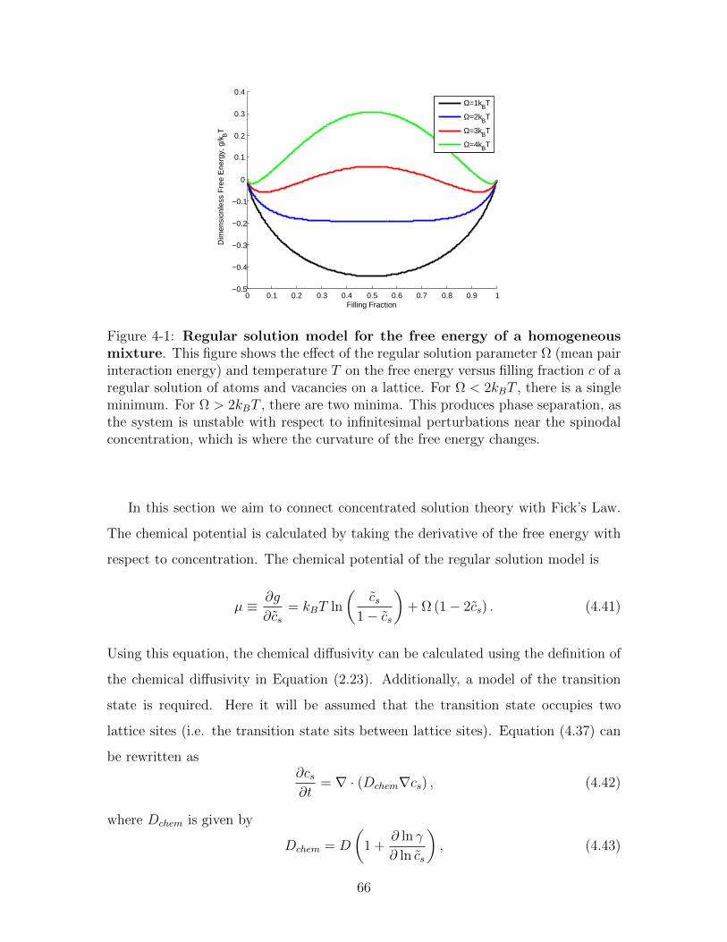
0 0.1 0.2 0.3 0.4 0.5 0.6 0.7 0.8 0.9 1−0.5

−0.4

−0.3

−0.2

−0.1

0

0.1

0.2

0.3

0.4

Filling Fraction

Dim

ensi

onle

ss F

ree

Ene

rgy,

g/k

BT

Ω=1kBT

Ω=2kBT

Ω=3kBT

Ω=4kBT

Figure 4-1: Regular solution model for the free energy of a homogeneousmixture. This figure shows the effect of the regular solution parameter Ω (mean pairinteraction energy) and temperature T on the free energy versus filling fraction c of aregular solution of atoms and vacancies on a lattice. For Ω < 2kBT , there is a singleminimum. For Ω > 2kBT , there are two minima. This produces phase separation, asthe system is unstable with respect to infinitesimal perturbations near the spinodalconcentration, which is where the curvature of the free energy changes.

In this section we aim to connect concentrated solution theory with Fick’s Law.

The chemical potential is calculated by taking the derivative of the free energy with

respect to concentration. The chemical potential of the regular solution model is

µ ≡ ∂g

∂cs= kBT ln

(cs

1− cs

)+ Ω (1− 2cs) . (4.41)

Using this equation, the chemical diffusivity can be calculated using the definition of

the chemical diffusivity in Equation (2.23). Additionally, a model of the transition

state is required. Here it will be assumed that the transition state occupies two

lattice sites (i.e. the transition state sits between lattice sites). Equation (4.37) can

be rewritten as∂cs∂t

= ∇ · (Dchem∇cs) , (4.42)

where Dchem is given by

Dchem = D

(1 +

∂ ln γ

∂ ln cs

), (4.43)

66

and D = Doγ/γTS. Substituting the regular solution chemical potential into Equa-

tions (4.42) and (4.43), along with the diffusivity definition, the chemical diffusivity

for the regular solution model is

Dchem,rs = Do

(2Ωc2

s − 2Ωcs + 1)

exp(

Ω (1− 2cs)), (4.44)

where Ω = Ω/kBT . In the dilute limit, we find that we obtain the dilute limit

diffusivity multiplied by some constant. This constant is related to the particle-

hole interaction energy given by Ω. Interestingly enough, this model recovers some

interesting phenomena for different values of Ω. For Ω < 0, the chemical diffusivity

increases and approaches a constant value at full filling. For Ω = 0, the dilute limit

(i.e. ideal) diffusivity is recovered. Finally, for Ω > 0, there is a minimum in the

diffusivity between zero and half filling. As Ω → 2kBT , the minimum diffusivity

approaches zero at half filling. Beyond 2kBT , the diffusivity is negative, indicative of

phase separation (i.e. “uphill diffusion”).

In order to simulate this regime, an additional energetic term is required. Uphill

diffusion is not only numerically difficult, it also doesn’t accurately represent exper-

imental data. When modeling phase separating systems, this negative diffusivity is

handled by using an additional gradient penalty, so that the problem is formulated

as diffusion down an energy gradient, instead of up a concentration gradient. This

method also more accurately represents experimental data. This is the purpose of the

Cahn-Hilliard free energy functional, which will be introduced in the next section.

4.4.2 The Cahn-Hilliard Free Energy Functional

The Cahn-Hilliard free energy functional includes a “gradient penalty” that stabilizes

the interface between phases of high and low concentration. Instead of apparent

uphill diffusion, which is numerically unstable, the resulting equation is always a

minimization in energy, and particles travel down the energy gradient. The functional

is

G[c(x)] =

∫V

[ρsg(c) +

1

2κ (∇c)2

]dV +

∫A

γs (c) dA, (4.45)

67

where ρs is the site density, g is the homogeneous free energy, κ is the gradient energy

(energy per length) and γs is the surface tension (energy per area). During phase sep-

aration, the gradient penalty controls the structure of the phase interface. Balancing

the terms in Equation (4.45) with the regular solution model as the homogeneous free

energy, it can be shown that the width of the phase interface scales as λi ≈√κ/Ω

and the interphasial tension scales as γi ≈ ρs√κΩ.

The concentrated solution theory formulation requires the chemical potential. To

calculate the chemical potential from the Cahn-Hilliard free energy functional (which

is a total free energy), the Euler-Lagrange variational derivative with respect to con-

centration is required. This is the continuum equivalent to the change in free energy

to add an atom to the system. The chemical potential per site is

µ =1

ρs

δG

δc= µ (c)−∇ ·

(κ

ρs∇c)

(4.46)

Inserting this chemical potential into concentrated solution theory flux in Equation

(4.36) and the overall conservation equation in Equation (4.37) results in a fourth

order partial differential equation. This higher order differential equation requires an

additional boundary condition. The additional boundary condition comes from the

variational calculus, and is given by

n · κ∇c =∂γs∂c

. (4.47)

This term ensures continuity of the chemical potential [32] and controls surface

wetting and nucleation. [8, 45, 44] Additional effects such as coherency strain can be

included in the Cahn-Hilliard model as well. If the surface term is neglected, but the

elastic strain energy and homogeneous component of the total strain are included,

the free energy equation becomes

G[c(x)] =

∫V

[ρsg(c) +

1

2κ (∇c)2 +

1

2Cijklεijεkl − σijεij

]dV. (4.48)

These additional effects of coherency strain can be approximated by a volume av-

68

eraged stress term. [36, 37, 38] The homogeneous component of the total strain

becomes1

2Cijklεijεkl ≈

1

2B (c−X)2 , (4.49)

where X is the volume averaged concentration. This term penalizes concentration

fluctuations from the volume averaged concentration and suppresses phase separation

depending on the value of B, which typically depends on orientation. [45] Including

this approximate strain term in the chemical potential as in Equation (4.46) yields

µ = µ−∇ ·(κ

ρs∇c)

+B

ρs(c−X) . (4.50)

This additional strain term effectively suppresses phase separation inside the nanopar-

ticles. The effects of different values of this parameter will be shown in model simu-

lations in later chapters. Adding the strain term represents just one of the additional

features that can be included in the solid particles. The benefit of this modified

porous electrode theory formulation is that any energetic model can be included, al-

lowing for more complicated phenomena such as phase separation and stress effects

to be modeled via simply changing the free energy function. This allows the same

framework to be used and prevents having to adapt the equations to artificially insert

these phenomena.

4.5 Non-dimensionalization and Scaling

At this point, the equations governing the dynamics of the battery system have all

been introduced. Mass and charge conservation equations govern the dynamics of

lithium inside the electrolyte. In the porous electrode, models of effective diffusivity

and conductivity are used for volume averaged continuum modeling. A modified

form of the Butler-Volmer equation along with the Nernst potential and the potential

drop in the solid conducting phase have also been presented. These terms allow the

reaction rate to be modeled throughout the electrode. Additionally, concentrated

solution theory can be used inside the solid particles, allowing more complicated

69

dynamics such as phase separation to be modeled in a coupled and self-consistent

manner.

Prior to solving these equations, however, suitable scalings allow dimensionless

quantities to be identified. These dimensionless quantities often govern the behavior

of the equations and allow different regimes to be identified. Additionally, proper

scaling makes the set of equations more numerically stable by removing some of the

stiffness associated with different time and length scales in the equations. This section

will deal with scaling of one of the electrodes. The scale can easily be extended to

the other electrode. It is important to note, though, that when scaling two electrodes

in this manner, a reference capacity is required. It is best to choose the smallest

capacity electrode as the scaling, so the total capacity of the cell is scaled to one.

Choosing the larger capacity electrode will lead to dimensionless currents that don’t

scale to one.

To begin, the total current (i.e. the integral of all fluxes times the area of the

particles) is scaled by the total electrode capacity. The total current is an integral

over the entire area of the solid, As, given by

I =

∫As

ejindAs =

∫Vs

eavjindVs. (4.51)

The term av, the interfacial area per particle volume, relates the solid interfacial area

to particle area. This is slightly different from the total particle area per electrode

volume, ap. The two terms are related via

ap = (1− ε)Lpav, (4.52)

where Lp is the volume fraction of the active material of the total solid volume. The

total current integrates over the entire solid volume in the electrode.

To scale the current, a time scale and charge scale are required. It is most con-

venient to use the diffusive time scale, td, and the total charge of the electrode. The

diffusive time scale is set by electrode length, L, and the dilute limit ambipolar dif-

fusivity, Damb,o. The time scale is td = L2/Damb,o. The total charge capacity of

70

the electrode is given by e (1− ε)LpV cs,max, where e is the charge per particle, ε

is the porosity, V is the total volume of the electrode, and cs,max is the maximum

concentration of lithium in the active material. The dimensionless current is

I =Itd

e (1− ε)LpV cs,max=

∫V

jindV . (4.53)

The dimensionless current is effectively a dimensionless C-rate. The term C-rate is

used for constant current battery discharge to denote the time in hours taken to

discharge the entire cell. An “n” C-rate is the same as discharging a cell in 1/n

hours. Since the diffusive time is on the order of 10 seconds, dimensionless C-rates

are typically much less than 1. A dimensionless C-rate of 0.003 is on the order of a

dimensional C-rate of 1. The dimensionless surface flux, jin is

jin =avjintdcs,max

. (4.54)

Next a proper scaling of the current density in the electrolyte is necessary. Since the

current density depends on the electrolyte concentration, it is scaled to the initial

electrolyte concentration, co. This is the concentration of lithium in the electrolyte

at open circuit conditions. The dimensionless current density is

i = −ε(Dchem,+ − Dchem,−

)∇c−

(z+D+ + z−D−

)εc∇φ, (4.55)

where the diffusivities have been scaled to the dilute limit ambipolar diffusivity. For

the case of a symmetric (i.e. z+ = z−) binary electrolyte, the dimensionless cation and

anion diffusivities are controlled by the transference number (Note: t+ + t− = 1 by

definition). The dimensionless diffusivities (for the symmetric case) can be expressed

as

D+ = (2t−)−1 , and (4.56)

D− = (2t+)−1 . (4.57)

71

Using these scalings, the dimensionless current density is given by

i =itdLeco

, (4.58)

where L is the length of the electrode. Next the charge conservation is non-dimensionalized.

The divergence of the current density is equal to the local charge consumption. Since

the electrolyte concentration is scaled to the initial electrolyte concentration, and the

reaction flux is scaled to the solid concentration, a scaling parameter remains after

non-dimensionalization. The charge conservation equation is

εβjin = −∇ · i, (4.59)

where β = Vscs,max/Veco, and represents the ratio of lithium in the solid to lithium in

the electrolyte at open circuit conditions. This parameter is important as it represents

the different regimes of charge storage. For β 1, the system behaves as a battery,

with high storage in the solid intercalation material. When β 1, the system behaves

like a super capacitor, which allows very fast charge storage. When β ∼ 1, the

system can be considered a pseudocapacitor, as this ratio of charge storage represents

a combination of surface storage and faradaic reactions.

Applying these scalings to the mass conservation equation, all scaling terms drop

out except for the β parameter. The dimensionless mass conservation equation is

ε∂c

∂t+ εβjin = ∇ ·

(εDamb∇c

)− ∇ ·

(t+i). (4.60)

All gradient operators are scaled by the electrode length, L, and the ambipolar dif-

fusivity is scaled by the dilute limit ambipolar diffusivity, Damb,o.

The solid diffusion equation must be scaled as well. The natural time scale in

the solid conservation equation is the solid diffusive time, L2s/Dchem, where Ls is

the length of the solid particle. However, since a single dimensionless time scale is

72

required, the parameter δd is introduced, which is a ratio of the diffusive time scales,

δd =L2sDamb

L2Ds,o

, (4.61)

where Ds,o is the dilute limit solid diffusivity (considered constant). Applying this to

the solid conservation equation, we obtain

δd∂cs

∂t= ∇s ·

(Dscs∇sµ

), (4.62)

where ∇s are the gradient operators scaled by the characteristic solid length scale,

Ls, cs is the solid concentration scaled by the maximum solid concentration cs,max,

Ds is the solid diffusivity scaled by the dilute limit solid diffusivity, Ds,o, and the

dimensionless chemical potential of the solid µ is scaled by the thermal energy, kBT .

This equation allows the solid dynamics to be modeled with respect to the diffusive

time chosen in the electrolyte conservation equation. The parameter δd scales inversely

with the solid diffusivity (i.e. slower diffusion is a larger δd) and proportionally with

the square of the characteristic solid particle length.

4.6 Conclusion

This chapter showed the derivation of the MPET equations as well as some free energy

equations and ways to handle phase separating materials. Table 4.1 lists the full set

of dimensional equations used in MPET along with suitable boundary conditions.

Other boundary conditions, such as the no-flux conditions for lithium at the current

collectors and walls of the electrodes, are not explicitly stated here. Depending on

the simulation (i.e. half cell or full cell) these boundary conditions are obvious. The

not as obvious boundary conditions, such as the flux into the separator, are given for

constant current discharge. In the case of constant potential discharge, the potential

boundary condition is held constant and the flux is varied to satisfy mass conservation.

Constant power discharge can also be performed by solving for the cell potential that

satisfies the constant power condition (i.e. the instantaneous potential multiplied by

73

the instantaneous current).

Equation Boundary Conditions

ε∂c∂t

+ apjin = ∇ · (εDamb∇c)−∇ ·(t+ie

)i|x=−δs = I/Asep

i = −e (D+ −D−) ε∇c−e2

kBT(z+D+ + z−D−) εc∇φ

jin = −∇·ieap

=

io

[exp

(− αeηkBT

)− exp

((1−α)eηkBT

)]

io = e(kocaO)1−α(koaaR)α

γ‡

η ≡ ∆φ−∆φeq

∆φeq = V o − kBTne

ln(aRaO

)∂cs∂t

= ∇ ·(DscskBT∇µ)

−DscskBT

∂µ∂r

∣∣∣r=R

= jin

Table 4.1: Dimensional set of equations. A list of the set of dimensional equationsfor Modified Porous Electrode Theory. The boundary conditions listed here are forconstant current discharge.

The conservation equation applies throughout the electrode volume. The current

density equation is used to calculate the potential drop in the electrolyte. This term is

important because it is required to calculate the observed potential, ∆φ. The reaction

rate equation, which is based on a modified form of the Butler-Volmer equation, is

used to calculate the reaction rate of the intercalation particles. This reaction rate

governs the flux of lithium into or out of the particles. This is the only way the

74

particles interact with the electrolyte. The dynamics inside the particles are handled

using concentrated solution theory. The type of coordinates for the particles should

be selected to best handle the particle geometry.

The Nernst potential of the intercalation particles is modeled using the same

thermodynamics used in the reaction rate and diffusion equations. This open circuit

potential is what controls the cell of the electrode as the particles fill. This feature is

what makes the MPET set of equations unique. The equations are fully self consistent

and the dynamics and potential of the cell are governed by the thermodynamics of the

material. While this is a strength of the model, this can also be problematic, because

the model itself relies on a thorough understanding of the material’s thermodynamic

properties in order to predict non-equilibrium dynamics. Neglecting one feature of

the material can result in a model which cannot fit experimental data. However, if

the thermodynamics are well known, then the model has the potential to provide a

much deeper understanding of the behavior of the material inside the electrode.

75

Chapter 5

Numerical Methods

Numerical methods are not the focus of this research, but it is necessary to comment

on which methods were used to solve the set of equations. The set of PDE’s was

reduced to a set of ODE’s using the finite volume method to approximate the spatial

derivatives. The problem was then formulated as a differential algebraic equation

(DAE) in order to solve the time integration. DAE’s consist of differential equations

(e.g. a time derivative) with algebraic constraints, which in this case are the charge

conservation conditions. Additionally, for the constant current, the integral of the

reaction rate is controlled (i.e. the potential that satisfies the current is simultaneously

solved for). For constant power discharge, the power is controlled (i.e. the potential

is solved for such that the product of the instantaneous potential and current is

constant).

This set of equations is well suited to be formulated as an index 1 DAE. The index

of a DAE is defined as the number of derivatives required to turn the equations into

an explicit ODE. Often the most difficult part of solving DAE’s is finding a consistent

set of initial conditions that satisfies the algebraic constraints. Higher index DAE’s

(i.e. index greater than 1) are difficult to solve because the initial conditions must

also satisfy derivatives of the constraints in the system. A brief overview of DAE

properties and solution approaches will be presented here. For more on DAE’s, DAE

index, and solution methods, the reader is directed to Ascher and Petzold. [4]

The solver used for this work is MATLAB’s ode15s, which is a variable first to

77

fifth order stiff equation solver. The solver uses a mass matrix formulation of the

DAE, which will be explained later in this chapter. First a brief overview of the finite

volume method will be presented, followed by a brief section on DAE formulation

using a mass matrix. Finally, an example of setting up a half cell for constant current

discharge will be given along with various constraints for different simulation types

(constant current, constant potential, constant power, etc.).

5.1 The Finite Volume Method

In this section, a brief overview of the centered finite volume method will be given.

The finite volume method conserves mass perfectly by tracking fluxes over the bound-

aries of a control volume. We refer to the method presented here as “centered” because

field variables (e.g. concentration and potential) represent values at the center of the

volume. Fluxes are therefore defined on the boundaries of the volume.

The advantage of this discretization method is that mass is perfectly conserved.

All fluxes in and out of a control volume are balanced with the local reaction rate

and accumulation term. For Neumann boundary conditions, setting the flux on the

boundary is straightforward. This can be accomplished by placing a dummy volume

outside the grid, or changing the value after the gradient is computed (i.e. altering a

value inside a “flux” vector).

Dirichlet boundary conditions require an approximation. Approximating the value

of a dummy volume outside the grid is one way to apply a Dirichlet boundary condi-

tion. As a rough first approximation, the dummy volume right outside the boundary

can be set to the boundary value. If higher accuracy is required, a Taylor approxima-

tion for this dummy volume can be used which takes into account the set value of the

boundary. Approximating a function f(x) using a Taylor expansion around x = a is

given by

f(x) ≈ f(a) +1

1!

df

dx

∣∣∣∣x=a

(x− a) +1

2!

d2f

dx2

∣∣∣∣x=a

(x− a)2 + ... (5.1)

78

Using finite difference methods to approximate the derivatives, an expression that

satisfies the boundary condition can be calculated for the dummy volume.

The finite volume method integrates the conservation equation over the discretized

volume. Consider a 1D conservation equation with no reaction rate and a constant

diffusivity, given by∂c

∂t= D

∂2c

∂x2. (5.2)

First, we consider a grid of discrete elements each with length ∆x. Integrating Equa-

tion (5.2) over the spatial direction, x, yields

∫ xo+∆x

xo

∂c

∂tdx =

∫ xo+∆x

xo

D∂2c

∂x2dx. (5.3)

Carrying out the integration over the length of the finite volume (i.e. xo to xo + ∆x)

and applying the Fundamental Theorem of Calculus, this equation becomes

∂c

∂t∆x =

(D∂c

∂x

∣∣∣∣xo+∆x

− D∂c

∂x

∣∣∣∣xo

)(5.4)

Next we divide both sides by ∆x. Then, recalling that the species flux is given by

F = −D∂c

∂x, (5.5)

we can substitute F into Equation (5.4) to obtain

∂c

∂t=Fin − Fout

∆x, (5.6)

where Fin is the flux at xo and Fout is the flux at xo+∆x. Here it can be seen that the

finite volume method is an application of Gauss’s Theorem to a control volume. By

tracking species fluxes across the boundaries of the control volume, as demonstrated

in Equation (5.6), the finite volume method conserves mass throughout the system.

This integration over the volume can be expanded to other geometries and grid

types as well. Consider the spherical coordinate diffusion equation in the radial

79

direction,∂c

∂t=D

r2

∂

∂r

(r2 ∂c

∂r

). (5.7)

Once again, both sides are integrated over the spatial direction, which in this case is

r. First, the r−2 term is moved to the time derivative side. The integration becomes

∫ ro+∆r

ro

r2∂c

∂tdr =

∫ xo+∆x

xo

D∂

∂r

(r2 ∂c

∂r

)dr. (5.8)

The time derivative can be pulled out of the derivative on the left side. Once again

the Fundamental Theorem of Calculus is applied to the right side. The integration

yields1

3r3

∣∣∣∣ro+∆r

ro

∂c

∂t=

(r2 ∂c

∂r

)∣∣∣∣ro+∆r

ro

. (5.9)

If we multiply the entire equation through by 4π, we recognize that the r3 term on the

left side is a volume and the r2 term on the right side is an area term. Substituting

∆V in to the equation and simplifying we obtain

∂c

∂t=

4π(r2 ∂c

∂r

∣∣ro+∆r

− r2 ∂c∂r

∣∣ro

)∆V

. (5.10)

Once again, we can substitute the flux terms in for the spatial derivatives. Also, the

area terms can be substituted. This yields the finite volume equation in the radial

direction in spherical coordinates,

∂c

∂t=AinFin − AoutFout

∆V. (5.11)

This example demonstrates how the finite volume method is capable of conserving

mass. The fluxes and respective areas are balanced and scaled by the volume of the

discrete element.

80

5.2 Differential Algebraic Equations

This section, as well as the next section, will loosely follow the work of Ascher and

Petzold. [4] The key property of a differential algebraic equation (DAE) is the

combination of differential equations and algebraic constraints. These constraints

could be a result of physical phenomena (e.g. conservation, continuity, etc.) or

additional constraints put on the system (e.g. constant current discharge). The most

general form of a DAE is

F(t,y,y′) = 0, (5.12)

where the function F returns a vector and the inputs are all vectors (denoted by

the bold typeface). This form can be broken down into a mass matrix formulation,

which is taken as the input for the solver used in this work, ode15s. The mass matrix

formulation combines the differential and algebraic equations into a single expression,

∂

∂t(My) = f (t,y) . (5.13)

In this equation, M is a rank 2 tensor. The mass matrix can be a function of time.

Furthermore, it can be singular. Here, it will be assumed that the mass matrix is

independent of time and can therefore be moved in front of the derivative,

M∂y

∂t= f (t,y) . (5.14)

This is the form preferred by MATLAB’s ode15s solver. The solver takes argu-

ments for the mass matrix, right hand side function (shown here as f), and is capable

of treating situations where the mass matrix is time dependent and/or singular. The

benefit of using a commercial package to solve the equations it that the software is

often tested rigorously and contains many additional features, such as adaptive time

stepping and error control properties.

However, the disadvantage is that when the solver fails, it’s difficult to know why

the solver failed. Frequently, it fails due to a mistake in the input. But sometimes,

parameter ranges produce errors for unknown reasons, and it may not be entirely clear

81

how to fix these errors. Additionally, commercial software packages often come with

distribution limitations, which could make it difficult to distribute the code to the

community. For this reason, it is often better to go with tested open source software

that is easily obtainable.

As was stated previously, numerical methods were not the focus of this research.

However, their importance cannot be overlooked, especially for the results presented

later in this thesis, which will demonstrate behavior not seen before in these types of

systems.

5.3 Solving DAE’s

One popular discretization method for the time derivative is the Backwards Differ-

entiation Formula (BDF). The BDF method fits a Newton polynomial to previous

time steps, then differentiates to obtain the term coefficients. BDF is an implicit

multi-step method, in that the next time step appears on both sides of the function.

To solve this, Newton’s method can be used.

Here we assume a constant mass matrix, and start with Equation (5.14). Let yn

represent the value we wish to solve for (that is, the values at the next time step).

The equation for the kth order BDF is

k∑i=0

αiyn−i − hβ0f (tn,yn) = 0, (5.15)

where α and β0 are parameters and h is the time step, ∆t. [4] Table 5.1 lists the

BDF coefficients for up to sixth order.

Upon closer inspection, it can be seen that first order BDF is the same as the

backwards Euler method. The summation term can be separated into two compo-

nents: the value at the next time step, and the value at previous time steps. Breaking

up the summation, Equation 5.15 becomes

yn + A− hβ0f (tn,yn) = 0, (5.16)

82

k β0 α0 α1 α2 α3 α4 α5 α6

1 1 1 -1

2 23

1 −43

13

3 611

1 −1811

911

− 211

4 1225

1 −4825

3625

−1625

325

5 60137

1 −300137

300137

−200137

75137

− 12137

6 60147

1 −360147

450147

−400147

225147

− 72137

10147

Table 5.1: BDF coefficients This table lists the BDF coefficients, for up to sixthorder (k is the order). This table is adapted from [4].

where

A =k∑i=1

αiyn−i. (5.17)

This separation demonstrates how the time derivative can be separated into the cur-

rent value (which is solved for and changes) and the previous time steps (which in the

summation) that are constant with respect to time. If we combine the BDF method

with the mass matrix DAE formulation in Equation (5.14), we obtain

F (tn,yn) = M (yn + A)− hβ0f (tn,yn) = 0. (5.18)

Next, Newton’s method is used to solve this equation for yn. Newton’s method

uses a Taylor expansion approximation to iterate towards the roots of the equation.

The Taylor expansion is

0 = yi+1n ≈ yin + J

(yin)

∆yn, (5.19)

where ∆yn = yi+1n − yin, is known as the Newton step. We wish to obtain the root of

the function, so the next iteration, yi+1n , is set to zero. Then, the equation is solved

for yi+1n , yielding

yi+1n = −J−1yin + yin, (5.20)

83

where the Jacobian, J, is defined as

Ji,j =∂Fi

∂yin,j. (5.21)

The Jacobian in Equation 5.21 is the derivative of the ith row of the output F with

respect to the jth component of the yin vector. The Jacobian of the left hand side of

Equation (5.18) is

J = M− hβ0Jf , (5.22)

where Jf is the Jacobian of the function f , in Equation 5.18. The purpose is to solve

for the next value, yi+1n . This can be accomplished either by inverting the Jacobian

(as in Equation 5.20), or using Gaussian elimination on Equation 5.19. This iteration

continues until some tolerance is reached, typically when the norm of the function is

below some absolute tolerance, atol, as in

||F(tn,y

i+1n

)|| ≤ atol. (5.23)

This is one method that can be used to solve the non-linear equation. MATLAB’s

ode15s uses a different implementation. For more on the method used by ode15s,

the reader is referred to [116]. In the last part of this chapter, an example of the

DAE formulation for the case of constant current will be presented.

5.4 DAE Formulation for Constant Current Dis-

charge

To demonstrate the DAE formulation, an example of a half cell discharged at constant

current will be presented. For this half cell, the pseudocapacitor approximation is ap-

plied, which allows diffusion in the solid particles to be neglected. The solid particles

are then replaced by sink terms (i.e. simple time derivatives). The metal potential

(φm) is set to 0 (reference potential) and it is assumed that electron transport is fast

84

(i.e. no potential drop for the electrons). The dimensionless equations become

ε∂c

∂t+ εβ

∂cs

∂t= ∇ ·

(ε∇c

), (5.24)

∂cs

∂t= −2io sinh

(η

2

), (5.25)

εβ∂cs

∂t= −∇ · i. (5.26)

This set of equations has three field variables: c, cs, and φ, which is inside the equation

for i. The spatial derivatives are handled using the finite volume method earlier in

this chapter. This DAE formulation focuses more on how to set up the mass matrix.

For this example, a simple 1D grid will be used, consisting of 3 volumes, with 1 in

the separator and 2 in the electrode. The anode is not modeled here and is treated as

having very fast kinetics. The electrolyte concentration, c, and electrolyte potential,

φ, exist throughout the separator and electrode, whereas the solid concentration, cs,

only exists in the electrode. There are no flux conditions at the end of the electrode

and a continuity condition at the electrode/separator interface. The flux of lithium

into the separator is set by the constant current (which is set in the simulation).

However, the electrolyte potential at the separator/anode boundary is unknown. This

value must be set to satisfy the constant current condition,

∫ 1

0

∂cs

∂tdx = I , (5.27)

where I is the constant dimensionless current (defined in Equation 4.53). In this

equation, x = 0 is the separator-anode interface and x = 1 is the cathode-current

collector interface.

Combining everything, there are 9 total variables: 3 field values of c, 3 field values

of φ, 2 field values of cs, and the potential boundary condition, φo. The mass matrix

has 81 values (most of them are 0). Rewriting Equations (5.24), (5.25), and (5.26)

into the form of Equation (5.14) becomes

85

ε − − − − − − − −

− ε − − − − εβ − −

− − ε − − − − εβ −

− − − − − − − − −

− − − − − − εβ − −

− − − − − − − εβ −

− − − − − − 1 − −

− − − − − − − 1 −

− − − − − − ∆x ∆x −

∂

∂t

c1

c2

c3

φ1

φ2

φ3

cs,1

cs,2

φ0

=

∇ ·(ε∇c

)∇ ·(ε∇c

)∇ ·(ε∇c

)−∇ ·

(i)

−∇ ·(i)

−∇ ·(i)

−2io sinh(η2

)−2io sinh

(η2

)I

. (5.28)

The equations on the right hand side should be discretized and represented using

the aforementioned finite volume method. The value for φ0 is the boundary condition

at the separator side. It is important to recognize that the mass matrix (the 9x9

matrix on the left) is singular. Furthermore, there are no time derivatives for the

potential conditions. These are the algebraic constraints set by the charge conserva-

tion. Additionally, the DAE controls the boundary condition via the constant current

condition (the last row). This equation can be formulated as Equation (5.18) and

solved via Newton’s Method.

5.5 Conclusion

The purpose of this chapter was to prevent a brief overview of DAE’s as they apply

to porous electrode theory and demonstrate how to formulate the set of equations

as a DAE. For the case of solid diffusion, then the solid concentration values in

Equation (5.28) should be replaced by the solid concentration inside the particles and

the reaction rate becomes the flux into the particles at the solid-electrolyte interface.

There are many different software packages available to solve DAE’s. This work

uses MATLAB’s ode15s because of its ease of use and robustness. Another good

86

solver to use is Assimulo in Python, which uses the Sundials (https://computation.

llnl.gov/casc/sundials/main.html) solver IDA. In the next chapter, some exam-

ple simulations will be presented. Later in this thesis, simulations will be compared

to experiment.

87

https://computation.llnl.gov/casc/sundials/main.html

https://computation.llnl.gov/casc/sundials/main.html

Chapter 6

Simulations

This chapter will present some example constant current simulations of the MPET

equations using the aforementioned ode15s. First, the case of homogeneous particles

will be considered. Various effects will be demonstrated including changing the dis-

charge rate, changing the exchange current density, and changing the solid diffusivity.

Additionally, phase separating particles will be considered. These particles will

be modeled in the surface reaction limit (SRL), allowing the depth concentration to

be neglected. The Cahn-Hilliard free energy functional will be used to model the

particles and stress effects will be considered. However, other important effects such

as surface wetting will not be considered in this section. For the case of no stress and

coherency strain, changes in the discharge rate will be demonstrated.

The values given in the simulation are dimensionless. Chapter 4 gives the scalings

for each of the values. Approximate dimensional values will be given in this chapter

as well to denote what regime the cell is in (e.g. fast/slow discharge). The figures

and results here are adapted from Ferguson and Bazant. [58]

6.1 Homogeneous Particles

The main features that will be investigated in this section are the discharge rate, the

exchange current density, and the solid diffusivity. The exchange current density is a

parameter that is often very difficult to accurately model. Many assumptions about

89

the reaction rate (i.e. the reaction steps and rate constants) are required. In phase

separating materials, where not all of the material’s surface area is necessarily active,

this can be even more difficult.

Prior to showing simulation results, it’s important to denote the axes used in the

figures. For the case of a 1D half cell, there are two directions lithium can diffuse

in: the depth direction into the electrode, and into the particles. These two axes are

combined into a signal contour plot which denotes the lithium concentration inside

the solid particles as well as the particles location inside the electrode. Figure 6-1

denotes the axes used in the homogeneous particle simulations.

x/L

x s/Lx,

s

Electrolyte diusion

Figure 6-1: Plot axes for diffusion-limited solid-solution particles. This figureshows how the simulation results below are plotted for porous electrodes with isotropicsolid solution particles. The y-axis of the contour plots represent the depth of theparticles while the x-axis represents the depth into the electrode. The particles aremodeled in 1D.

For these simulations of homogeneous particles, a porosity of 0.4 was used. The

dimensionless parameter εβ was set to 22.8, which is a little larger than typical elec-

trodes, and is used to demonstrate electrolyte depletion. The volume percent of active

material was set to 0.7. This results in a max concentration of 54 M lithium in the

solid.

Ion diffusivities in the electrolyte were considered constant and taken from Valoen

and Reimers [136]. The cation diffusivity was set to 1.25e-10 m2/s and the anion

diffusivity was 4e-10 m2/s, which results in an ambipolar diffusivity of 1.9e-10 m2/s.

The electrode length was 50 µm and the particles were plate-like particles that are 50

90

nm x 200 nm x 100 nm thick (half of this was modeled, and a symmetry boundary

condition is used at the center), with the top and bottom as active surfaces. The

charge transfer coefficient is set to 0.5. The separator is assumed to be 25 µm thick.

The electrode is discretized into 20 volumes and the separator is discretized into 10

volumes. The solid particles were discretized into 50 volumes. The dimensionless

exchange current density was 0.01, which corresponds to a dimensional exchange

current density of approximately 0.2 A/m2.

The first simulation demonstrates the effect of increasing the current. In these

particles, the ratio of diffusive times, δd, is given by Equation 4.61. It is set to one in

this simulation so that solid diffusion has the same diffusive time as the electrode. This

gives fast diffusion in the solid. The result is that the voltage dropoff is caused by an

electrolyte limitation. Figure 6-2 shows the voltage diagrams and solid concentration

profiles for different discharge rates.

A dimensionless current of 0.001 is equivalent to a dimensional discharge rate of

approximately C/3. The other dimensionless current values of 0.01 and 0.05 are ap-

proximately 3C and 15C, respectively. The red dots on the voltage curves correspond

to the solid concentration profiles, from top to bottom, left to right in the figures

below. At the slowest discharge rate, the particles fill homogeneously throughout

the electrode. As the current is increased, it can be seen that particles closer to the

separator (on the left) have a higher lithium concentration than particles deeper in

the electrode. At the fastest discharge rate, there is a large difference between parti-

cles next to the separator and particles deeper in the electrode. The voltage drop-off

in the fastest discharge curve is actually due to an electrolyte transport limitation.

Figure 6-3 demonstrates this depletion.

Figure 6-3 shows the voltage curve for the 15C discharge in figure 6-2. The three

dots correspond to the diagrams below which show the solid concentration profiles

throughout the electrode (left) and the electrolyte concentration (right), including

the separator (note: the discontinuity is the separator/electrode interface and the

slope change is the result of a porosity change). The figures show how the electrolyte

depletes, resulting in increased overpotential. This proceeds until the electrolyte is

91

0 0.1 0.2 0.3 0.4 0.5 0.6 0.7 0.8 0.9 13

3.1

3.2

3.3

3.4

3.5

3.6

Filling Fraction

Vol

tage

i=0.001i=0.01i=0.05

x s / L x,

s

x / L0 0.2 0.4 0.6 0.8 1

0

0.5

1

x s / L x,

s

x / Lx

0 0.2 0.4 0.6 0.8 10

0.5

1

x s / L x,

s

x / L0 0.2 0.4 0.6 0.8 1

0

0.5

1

x s / L x,

s

x / L0 0.2 0.4 0.6 0.8 1

0

0.5

1

x s / L x,

s

x / L0 0.2 0.4 0.6 0.8 1

0

0.5

1

x s / L x,

s

x / L0 0.2 0.4 0.6 0.8 1

0

0.5

1

Figure 6-2: Effect of current on homogeneous particles. This figure demon-strates the effect of different discharge rates on the voltage profile. The non-dimensional currents correspond to roughly C/3, 3C, and 15C. The solid diffusionis fast, with δd = 1.

92

0 0.1 0.2 0.3 0.4 0.5 0.6 0.7 0.8 0.9 13

3.05

3.1

3.15

3.2

3.25

3.3

3.35

3.4

3.45

3.5

Filling Fraction

Vol

tage

x s / L x,

s

x / L0 0.5 1

0

0.5

1

−0.5 0 0.5 10

1

2

3c

/ c0

x / L

x s / L x,

s

x / L0 0.5 1

0

0.5

1

−0.5 0 0.5 10

1

2

3

c / c

0

x / L

x s / L x,

s

x / L0 0.5 1

0

0.5

1

−0.5 0 0.5 10

1

2

3

c / c

0

x / L

Figure 6-3: Depletion of the electrolyte at higher current. This figure shows thedepletion of the electrolyte accompanying Figure 6-2 for the 15C discharge. The leftfigure shows the solid concentration while the right figure demonstrates the electrolyteconcentration profile in the separator and electrode.

93

completely depleted, at which point the constant current can longer be sustained,

leading to a sharp drop off in potential.

Next, the effect of slower solid diffusion is considered. To control solid diffusion,

the value of δd is varied. This parameter is the ratio of the diffusive time of the

solid to that of the electrolyte (given by Equation 4.61). Typically, this value is

larger than one, but it scales with the solid diffusivity (a material property) and the

particle size. The solid diffusivity usually needs to be fit. Figure 6-4 demonstrates

the effect of increasing current on particles with slower solid diffusion. The δd value

has been changed from 1 to 100, meaning the solid diffusion time (L2s/Ds) is 100 times

larger than the electrolyte diffusive time (L2/Damb). This leads to a solid transport

limitation, causing lithium to build at the surface of the particles, leading to increased

overpotential.

Figure 6-4 shows the same discharge rates as Figure 6-2 but with slower solid

diffusion. The three red dots correspond to the solid concentration profiles below,

left to right, top to bottom. At C/3 discharge (I = 0.001), the particles fill homo-

geneously throughout the electrode. As the current is increased to 3C, the particles

start to exhibit concentration gradients throughout the electrode. Eventually, high

concentrations at the surface of the particles lead to increased overpotential and a

voltage dropoff around half filling. At 15C, this effect is even more pronounced, lead-

ing to a sharp voltage dropoff near 10% filling. This figure demonstrates the model’s

sensitivity to solid diffusivity and demonstrates how reduced solid transport affects

the cell voltage.

Next, the effect of solid diffusivity will be demonstrated for a single current. Figure

6-5 demonstrates the effect of solid diffusivity at a discharge rate of 3C. Here the effect

of decreasing the solid diffusivity is much more pronounced. By increasing the value

of δd from 1 to 100, half the capacity of the cell is lost. This change in δd corresponds

a solid diffusion pathway that is 10 times longer, or a solid diffusivity that is reduced

by a factor of 100. Even a value of δd = 50, which represents a solid diffusion pathway

approximately 7 times longer, or a solid diffusivity that is reduced by a factor of 50,

shows a decrease of 20% capacity.

94

0 0.1 0.2 0.3 0.4 0.5 0.6 0.7 0.8 0.9 13

3.1

3.2

3.3

3.4

3.5

3.6

Filling Fraction

Vol

tage

i=0.001i=0.01i=0.05

x s / L x,

s

x / L0 0.2 0.4 0.6 0.8 1

0

0.5

1

x s / L x,

s

x / L0 0.2 0.4 0.6 0.8 1

0

0.5

1

x s / L x,

s

x / L0 0.2 0.4 0.6 0.8 1

0

0.5

1

x s / L x,

s

x / L0 0.2 0.4 0.6 0.8 1

0

0.5

1

x s / L x,

s

x / L0 0.2 0.4 0.6 0.8 1

0

0.5

1

x s / L x,

s

x / L0 0.2 0.4 0.6 0.8 1

0

0.5

1

Figure 6-4: Effect of current on homogeneous particles with slower soliddiffusion. This figure demonstrates the effect of different discharge rates on thevoltage profile. The non-dimensional currents correspond to roughly C/3, 3C, and15C. The solid diffusion is slower than the electrolyte diffusion (δd = 100).

95

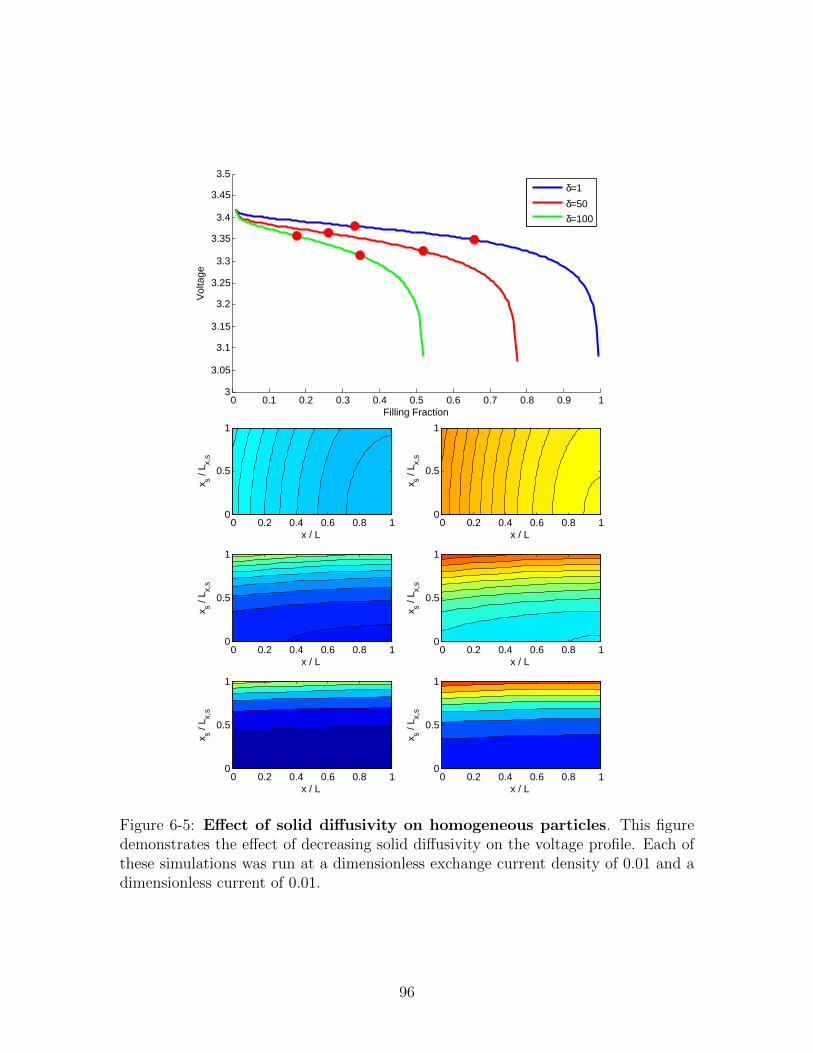
0 0.1 0.2 0.3 0.4 0.5 0.6 0.7 0.8 0.9 13

3.05

3.1

3.15

3.2

3.25

3.3

3.35

3.4

3.45

3.5

Filling Fraction

Vol

tage

δ=1

δ=50

δ=100

x s / L x,

s

x / L0 0.2 0.4 0.6 0.8 1

0

0.5

1

x s / L x,

s

x / L0 0.2 0.4 0.6 0.8 1

0

0.5

1

x s / L x,

s

x / L0 0.2 0.4 0.6 0.8 1

0

0.5

1

x s / L x,

s

x / L0 0.2 0.4 0.6 0.8 1

0

0.5

1

x s / L x,

s

x / L0 0.2 0.4 0.6 0.8 1

0

0.5

1

x s / L x,

s

x / L0 0.2 0.4 0.6 0.8 1

0

0.5

1

Figure 6-5: Effect of solid diffusivity on homogeneous particles. This figuredemonstrates the effect of decreasing solid diffusivity on the voltage profile. Each ofthese simulations was run at a dimensionless exchange current density of 0.01 and adimensionless current of 0.01.

96

This section provided examples of homogeneous particle behavior with different

discharge rates and solid diffusivity values. The next section will cover phase sepa-

rating particles.

6.2 Phase Separating Particles

The model presented here inside the MPET framework is the surface reaction limited

(SRL) model first presented by Bai et al.. [8] This model was applied to lithium

iron phosphate (LFP) particles. While the simulations presented here are similar,

different values were used for the gradient penalty, κ. Additionally, coherency strain

will be approximated later in the section. These results are not intended to accurately

capture the behavior of LFP in a porous electrode.

Accurately modeling LFP requires additional effects, including surface wetting

and particle size effects. [45, 44] Also, since LFP is not a good electrical conductor,

electron transport in the porous media, and possibly even the carbon coating of

the individual nanoparticles, could play an important role. In the next chapter, a

model based on these effects to describe the small current voltage gap observed in

LFP electrodes will be presented and compared to data. [54] For now, though, the

simplified case will be presented to demonstrate the model’s ability to use phase field

models to model phase separating materials.

Figure 6-6 shows how the solid concentration data is presented in this section. In

the previous section, the y-axis denoted the particle’s solid concentration in the depth

direction. In this section, it is assumed that the depth direction has fast diffusion,

allowing the particles to be depth averaged. [96] The y-axis in the contour plots

shown display the solid concentration across the surface of the particles. The x-axis,

as before, shows the particle’s location relative to the separator.

The same electrolyte transport properties were used as for the homogeneous par-

ticles. The length of the electrode was 50 µm, with a separator length of 25 µm. The

value of εβ was 24. The particle dimensions were assumed to be 50 nm x 50 nm x 30

nm (30 nm is the depth), with one active surface. A dimensionless exchange current

97

x/L

ys/Ly,s

Electrolyte diusion

Figure 6-6: Plot axes for reaction-limited phase separating particles. Thisfigure shows how the results are plotted below for porous electrodes with reaction-limited phase separating nanoparticles. The y-axis of the contour plots represent thelength along the surface of the particle, since diffusion is assumed to be fast in thedepth direction. The x-axis represents the depth in the electrode.

density of 0.1 was used, which corresponds to an exchange current density of approxi-

mately 1.25 A/m2. The value of the dimensionless gradient penalty, κ = κ/kBTρsL2s,

was 0.001. For the case of an approximated bulk coherency strain, the dimensionless

parameter b = b/kBTρs, was set to 1.6. The porosity was set to 0.4.

Three results will be presented to demonstrate the effect of increasing the discharge

rate and adding coherency strain. First, a slow discharge curve is presented (C/30).

Then an approximate coherency strain term is added. This term suppresses phase

separation. Finally, the effect of increasing the discharge rate is demonstrated.

Figure 6-7 shows the effect of slowly discharging the phase separating particles.

The discharge rate corresponds to approximately C/30. While a single particle would

have a strong tendency to phase separate at this discharge rate, a porous electrode

of these particles (all uniform in size) does not exhibit the same behavior. Instead,

a sharp front emerges that separates filled and empty particles, and the particles

undergoing lithiation fill quickly and homogeneously. It is not until the end of the

simulation, where single particle behavior becomes more evident (since the number

of remaining particles is small), that phase separation occurs.

One way to explain this is that the local current density is actually much larger

than the total current of the cell. Bai et al. demonstrated that for single particles

98

Figure 6-7: Phase separating particles slowly discharged. This figure showsslow discharge (approx. C/30) of phase separating particles. Adequate electrolytediffusion and discrete filling don’t allow time for the particles to phase separate earlyon. At the end of the discharge, sufficient time allows the particles to phase separate.

99

(using the same model here), if the local current density is much less than the exchange

current density, phase separation occurs. [8] While the total current (i.e. the integral

of the reaction rate over all the particles) is less than the exchange current density, the

local current density shown here is not. This leads to particles filling homogeneously

and discretely.

Not only do the particles at the front fill discretely, but low concentration particles

actually delithiate while these particles are filling. This is due to the non-monotonic

shape of the open circuit voltage profile of the material when it behaves homoge-

neously. The particle voltage oscillates between the miscibility and spinodal concen-

trations. The flat voltage plateau produced in the figure is the result of the difference

between the miscibility voltage and spinodal voltage. There is a finite overpotential

that is required before the particles can be lithiated. On lithiation, there is also a

finite overpotential required to drive lithiation. In the limit of zero current, this pro-

duces a “voltage gap”, which was explained by Dreyer et al.. [54] This simulation

demonstrates the importance of particle-particle effects in the cell.

It was later shown by Cogswell and Bazant that coherency strain on lithiation can

further suppress the phase separation of these particles. [45] To simulate this system,

an additional coherency strain energy penalty was included. This additional term

penalizes deviations from the particles average concentration, which promotes homo-

geneous filling. Figure 6-8 demonstrates the effect of this additional energy penalty.

At the same C/30 discharge rate, this additional penalty term further suppresses

phase separation in the particles, and all particles fill homogeneously throughout the

electrode.

Another effect to be demonstrated is the current induced suppression of phase

transformation at the porous electrode scale. This idea was first introduced by Bai et

al.. It was shown that as current is increased for a single particle, phase separation is

suppressed, leading to homogeneous filling. [8] Interestingly enough, a similar effect

can be seen on the porous electrode scale. If we consider discrete filling to be similar

to phase separation (i.e. when particles fill discretely, it’s similar to having lithiated

and delithiated regions with an active region between them), then the same effect is

100

Figure 6-8: Phase separating particles including coherent stress effectsslowly discharged. This figure shows slowly discharge (approx. C/30) phase sep-arating particles. The inclusion of the coherent stress effects suppresses phase sepa-ration inside the particles. This figure is the same as Figure 6-7, with an additionalcoherent stress term.

101

observed on the electrode scale. As the discharge rate is increased, the number of

active particles in the electrode increases. This number increases until all the particles

in the electrode are active, at which point the electrode fills homogeneously.

Interestingly enough, this occurs when the dimensionless current is roughly on the

order of the dimensionless exchange current, which is similar to the results observed

by Bai et al.. [8] Figure 6-9 shows discharge at a dimensionless current of 0.01,

which is approximately 3C. The increased discharge rate increases the number of

active particles, and instead of discrete filling of individual particles, discrete filling

of clusters of particles is observed. The number of particles increases until the entire

electrode fills homogeneously. This behavior is very different from the slow discharge

case. This effect can be described with an equivalent circuit model.

Figure 6-10 shows an equivalent circuit for the porous electrode. Each particle

can be characterized using a representative time scale for charge/discharge. This time

scale, tc, can be expressed as

tc ∼ RctCp, (6.1)

where Rct is non-linear charge transfer resistance, and Cp is the non-linear capaci-

tance. These values are non-linear, as they will vary based on filling, location, and

other particle properties. The number of active particles, nap, should scale with the

dimensionless current,

nap ∼ tcI . (6.2)

As the discharge rate is increased, the number of active particles scales as well. For

fast kinetics (or slow discharge rates), the number of active particles is small, leading

to discrete filling of the particles. Slower kinetics (or fast discharge rates) requires

more active particles to sustain the discharge rate, leading to a larger number of

active particles.

102

Figure 6-9: Effect of current on phase separating particles. When discharged ata higher C-rate (in this example, 3C), the size of the discrete particle filling is larger,leading to more particles filling simultaneously and a voltage curve that resemblessolid solution behavior.

103

Figure 6-10: Equivalent circuit model for a porous electrode. This equivalentcircuit represents a typical porous electrode in cases without significant electrolytedepletion, where the pore phase maintains nearly uniform conductivity. Resistorsrepresent the contact, transport, and charge transfer resistances, and the capacitanceof the particles is represented by a capacitor. All elements are not necessarily linear.

6.3 Conclusion

These results demonstrate the behavior of the model for phase separating and ho-

mogeneous solid materials in the porous electrode. For homogeneous materials, the

discharge is sensitive to solid diffusivity and concentration gradients inside the parti-

cles can lead to large overpotentials. The simulations also demonstrated the effect of

increasing the discharge rate and depleting the electrolyte. The simulations of phase

separating materials demonstrated the effect of the current on how the electrode fills.

They also showed how coherency strain inside these phase separating particles can

suppress phase separating. While this is the case for uniform electrodes (i.e. all par-

ticles have the same shape/size), results in the next two chapters will demonstrate

how particle size can break this symmetry, leading to preferential filling of particles

deeper in the electrode.

For application to real phase separating systems, such as LiFePO4, more compli-

cated models of the solid material are required. Recent work by Cogswell and Bazant

demonstrated that surface wetting and coherency strain can play a large role in the

overpotential required to lithiate LFP particles. [44] They found that the side facets

of LFP energetically prefer to be wetted (i.e. lithiated). The ratio of the wetted

surface area to the volume of the particle, combined with coherency strain, causes

smaller particles to preferentially fill. This model will be incorporated into the MPET

104

framework later in this thesis and qualitatively compared with experiments.

In the next chapter, comparison with experiments will be presented. First, an LFP

electrode will be simulated using a simplified form of Cogswell and Bazant’s model

along with the MPET framework to fit the small current voltage gap experiments

by Dreyer et al.. [54] The model demonstrates the importance of size effects in the

electrode. Additionally, a new graphite model will be presented and used to fit the

experiments of Harris et al.. [67] Harris “unrolled” a graphite electrode and put a

glass slide on top to observe the color change associated with lithiation of the graphite.

The free energy model, along with MPET, are used to fit the observed color profiles.

105

Chapter 7

Modeling Phase Separating

Materials

In this chapter, the Modified Porous Electrode Theory framework is applied to two

representative porous electrode experiments: (i) surface reaction-limited intercalation

in LFP, and (ii) electrolyte-diffusion limited intercalation in graphite. The analysis is

based on a general Cahn-Hilliard phase-field porous electrode model, as presented in

this thesis. Although the conclusions also follow from the full model, simulations and

analysis of the “pseudocapacitor” limit of homogeneous intercalation in each particle

are presented. This limit can be caused by fast diffusion and/or suppressed phase

separation compared to experimental time scales.

7.1 Reaction-Limited Dynamics with Two Phases

This section builds on the work of Cogswell and Bazant, which showed that surface

wetted nucleation combined with coherency strain (SWCS) reproduces many of the

phenomena observed in LFP nanoparticles. [44] While this model addresses many of

the interesting particle scale effects, many questions remain about dynamics at the

scale of the porous electrode. The SWCS model is very computationally expensive. To

explore the effects of hundreds of these particles inside a porous electrode, reduction

of the model is necessary so that simulations can be run on a reasonable time scale

107

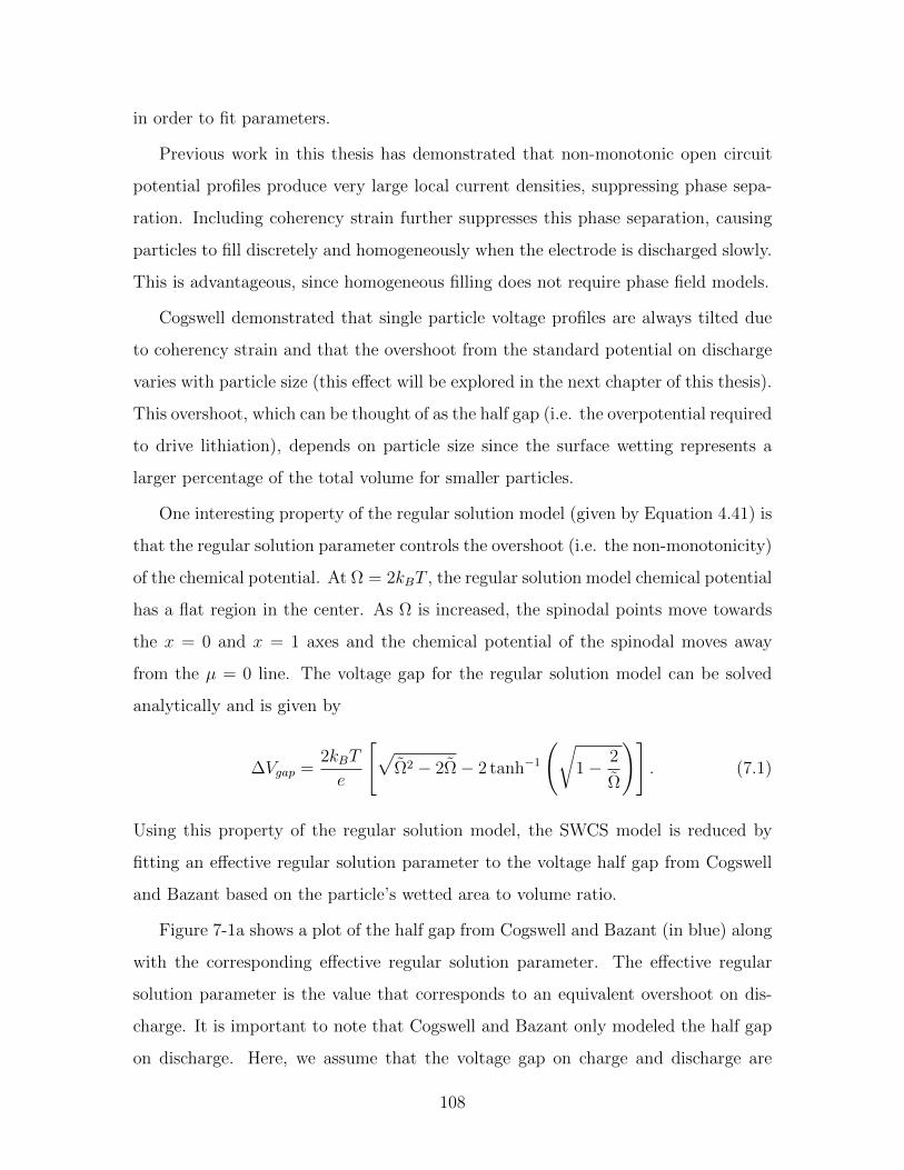
in order to fit parameters.

Previous work in this thesis has demonstrated that non-monotonic open circuit

potential profiles produce very large local current densities, suppressing phase sepa-

ration. Including coherency strain further suppresses this phase separation, causing

particles to fill discretely and homogeneously when the electrode is discharged slowly.

This is advantageous, since homogeneous filling does not require phase field models.

Cogswell demonstrated that single particle voltage profiles are always tilted due

to coherency strain and that the overshoot from the standard potential on discharge

varies with particle size (this effect will be explored in the next chapter of this thesis).

This overshoot, which can be thought of as the half gap (i.e. the overpotential required

to drive lithiation), depends on particle size since the surface wetting represents a

larger percentage of the total volume for smaller particles.

One interesting property of the regular solution model (given by Equation 4.41) is

that the regular solution parameter controls the overshoot (i.e. the non-monotonicity)

of the chemical potential. At Ω = 2kBT , the regular solution model chemical potential

has a flat region in the center. As Ω is increased, the spinodal points move towards

the x = 0 and x = 1 axes and the chemical potential of the spinodal moves away

from the µ = 0 line. The voltage gap for the regular solution model can be solved

analytically and is given by

∆Vgap =2kBT

e

[√Ω2 − 2Ω− 2 tanh−1

(√1− 2

Ω

)]. (7.1)

Using this property of the regular solution model, the SWCS model is reduced by

fitting an effective regular solution parameter to the voltage half gap from Cogswell

and Bazant based on the particle’s wetted area to volume ratio.

Figure 7-1a shows a plot of the half gap from Cogswell and Bazant (in blue) along

with the corresponding effective regular solution parameter. The effective regular

solution parameter is the value that corresponds to an equivalent overshoot on dis-

charge. It is important to note that Cogswell and Bazant only modeled the half gap

on discharge. Here, we assume that the voltage gap on charge and discharge are

108

the same. Figure 7-1b demonstrates representative open circuit potential profiles for

different sized particles.

This reduction of the SWCS model allows multiparticle simulations to be per-

formed using the MPET framework. The experimental work that will be focused on

here is the work of Dreyer et al., which observed a non-zero voltage gap in the limit of

zero current. [54] The paper showed a voltage gap of 20 mV remained at charge/dis-

charge rates of ±C/1000. The benefit of this experiment is its extremely slow charge

and discharge rate, which allows particle-particle interactions to be examined without

the effects of transport limitation or high overpotentials.

The work of Dreyer et al. represents one of the first major steps towards under-

standing the lithiation dynamics of an LFP electrode. The authors suggested that

the non-monotonic open circuit potential profile was the source of the voltage gap.

However, a regression with thermodynamic data by Cogswell and Bazant suggests

that the equilibrium voltage gap in homogeneous particles is on the order of 74 mV.

[45] Cogswell and Bazant went on to predict that the discrepancy in the voltage gap

is caused by the wetted area to volume ratio, which depends on particle size. Using

the reduced SWCS model along with MPET, the model is capable of reproducing the

voltage curves as well as the voltage gap with only three fitting parameters: average

particle size, particle size variance, and a constant contact resistance.

Given the slow charge/discharge rates, electrolyte properties are not very impor-

tant since the electrolyte does not deplete. For completeness, however, suitable num-

bers were chosen for transport properties. An ambipolar diffusivity of 1.5x1010m2/s

was used for the 1M LiPF6 in EC/DEC electrolyte. [125] A transference number

could not be found for this electrolyte, so a value of 0.35 was assumed, which is in

line with other typical battery electrolytes. [1] The electrode was assumed to be 50

µm long with a 25 µm separator. The volume fraction of the active material was

assumed to be 0.5, and the porosity was 0.4. It is important to iterate that at such

slow charge/discharge rates, there is no electrolyte depletion and these values have

little to no effect on the simulations.

Calculation of the particle size was performed using a random normal distribution.

109

0 0.05 0.1 0.15 0.2 0.25

0.01

0.02

0.03

0.04∆φ

* (V)

Wetted Area/Volume (nm −1)

2.5

3

3.5

4

4.5

5

Ωe

/kB

T

0 0.2 0.4 0.6 0.8 1−0.05

0

0.05

Filling Fraction

Vo−V

o (V)

20 nm30 nm50 nm500 nm

a)

b)

Figure 7-1: Voltage half gap and effective regular solution. Figure a denotesthe voltage half gap on discharge from Cogswell and Bazant and the resulting ef-fective regular solution parameter as a function of the wetted area to volume ratio.Figure b demonstrates various effective open circuit potential profiles for differentsized particles.

110

The particle shapes were assumed to be the C3 shape from Cogswell and Bazant. [44]

This shape was derived from Smith et al.. [121] The particles were assumed to be

20 nm thick. [121, 115] Calculation of the wetted surface area to volume ratio

was calculated via A/V = 3.6338/d, where d is the size of the particle in the [100]

direction. [44] The exchange current density used in the simulation was 1.5 A/m2.

The actual value of this parameter should not be taken literally, as will be explained

later. A normal distribution was used to generate the particle sizes.

The simulation was run by starting with a fully charged electrode, which was then

discharged to a filling fraction of 0.2 at a C/10 rate. The electrode was then relaxed by

simulating a zero current for a long period of time (roughly 3.5 hours in dimensional

time). The electrode was then discharged to a filling fraction of 0.7, relaxed, then

charged back to 0.2. When calculating the voltage gaps, the data were smoothed

(since discrete particle filling makes the data very noisy, although the fluctuations are

very small) to make the value consistent. A constant contact resistance was used to

fit the data. A value of 3.9 Ω·g was found to fit the data the best.

Figure 7-2 compares simulation results with the data from Dreyer et al.. Figure

7-2a overlays the voltage data on the simulation data for discharge rates of C/1000,

C/200, and C/131. The simulation filling range was extended due to start up effects

from the discreteness of the model. The model shows good agreement with the

discharge voltage data, even matching the slope of the voltage curves. On charging,

however, the agreement is not as good. While the model predicts more symmetric

behavior on charge and discharge, the experimental data shows overlapping between

the C/200 and C/131 charging data.

An important parameter in the simulation to mention is the exchange current

density. The exchange current density used in the simulation is 1.5 A/m2. While this

value seems very high compared to other values in simulations, the difference is that

this value is per active area. Determining the active area in a real system is very

difficult unless a single particle is discharged. Given the discrete nature of the model,

the active area is a very small fraction of the entire electrode. Other simulations,

such as traditional porous electrode theory, assume the entire electrode is active, and

111

0.2 0.3 0.4 0.5 0.6 0.73.4

3.41

3.42

3.43

3.44

3.45

Filling Fraction

Volta

ge (V

)

ModelData

0 0.05 0.1 0.15 0.20

1

2

3

4

5x 10−3

Voltage Gap (V)

Curr

ent (

A/g

)

µ=30,σ=5No size dependenceData

0.35 0.4 0.45 0.5 0.55 0.63.406

3.407

3.408

3.409

3.41

3.411

3.412

Filling Fraction

Volta

ge (V

)

σ = 1σ = 5σ = 10Data

Sepa

rato

rSe

para

tor

Sepa

rato

r

20 30 40Particle Size, 010 Plane (nm)

µ=30,σ=5 Histogram

σ = 1

σ = 5

σ = 10

a) b)

d)c)

Depth into electrode

Figure 7-2: Voltage gap fit to data. This figure shows the fit of the model toexperimental data from Dreyer et al. [54] Figure (a) shows an overlay of the simu-lation with the data for C/1000, C/200, and C/131. Figure (b) shows the effect ofparticle size variance on the voltage curve. Figure (c) compares the voltage gap todata with the additional C/100 and C/50 rates. Also the voltage gap with no sizeeffect is demonstrated. The inlay shows the particle size distribution used to fit thedata. Figure (d) shows representative particle sizes for the variances given in figure(b) at a filling fraction of 0.5. Experimental data in figures (a-c) from [54], providedcourtesy of Miran Gaberscek

therefore treat the entire electrode area in the exchange current. This can produce

a large difference in the exchange current density, on the order of many orders of

magnitude. For example, values from Srinivasan and Newman [123] indicate a total

electrode area of approximately 0.1 m2, compared to these simulations, which predict

an active area on the order of 0.0004 m2 (for 30 nm C3 shaped particles).

The actual value of the exchange current density is not important as long as the

value remains larger than the local current density. When the local current density is

less than the exchange current density, a particle-by-particle effect is observed which

112

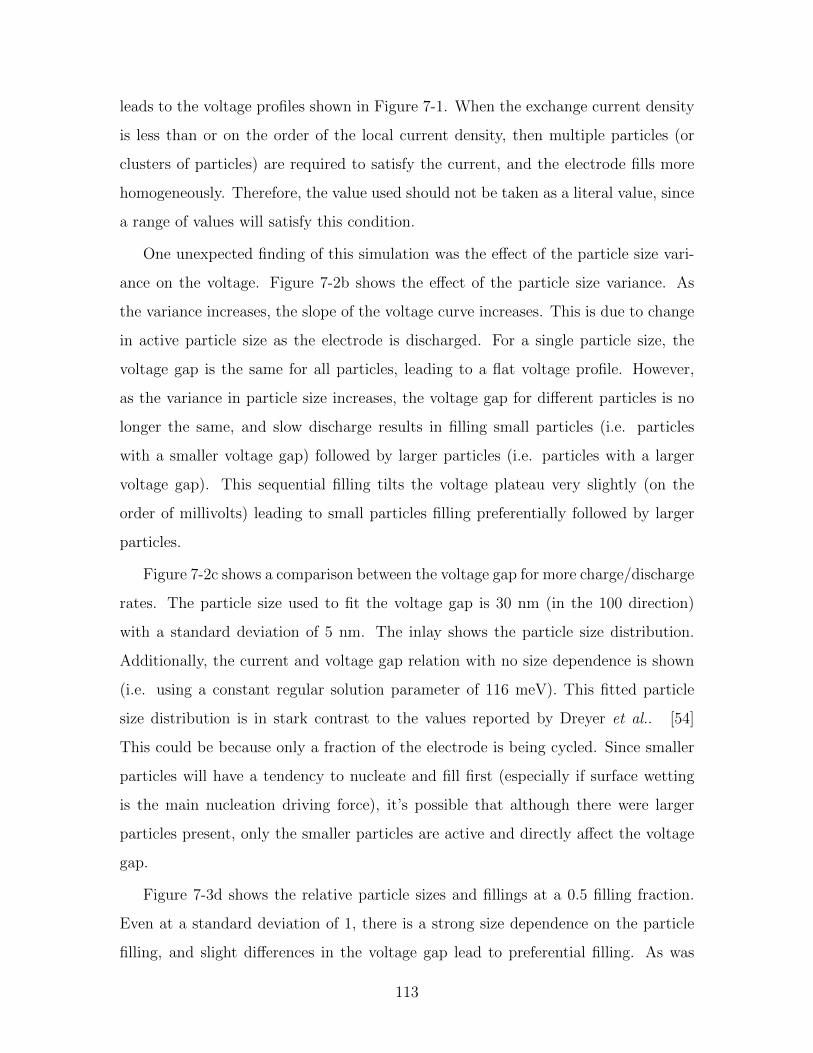
leads to the voltage profiles shown in Figure 7-1. When the exchange current density

is less than or on the order of the local current density, then multiple particles (or

clusters of particles) are required to satisfy the current, and the electrode fills more

homogeneously. Therefore, the value used should not be taken as a literal value, since

a range of values will satisfy this condition.

One unexpected finding of this simulation was the effect of the particle size vari-

ance on the voltage. Figure 7-2b shows the effect of the particle size variance. As

the variance increases, the slope of the voltage curve increases. This is due to change

in active particle size as the electrode is discharged. For a single particle size, the

voltage gap is the same for all particles, leading to a flat voltage profile. However,

as the variance in particle size increases, the voltage gap for different particles is no

longer the same, and slow discharge results in filling small particles (i.e. particles

with a smaller voltage gap) followed by larger particles (i.e. particles with a larger

voltage gap). This sequential filling tilts the voltage plateau very slightly (on the

order of millivolts) leading to small particles filling preferentially followed by larger

particles.

Figure 7-2c shows a comparison between the voltage gap for more charge/discharge

rates. The particle size used to fit the voltage gap is 30 nm (in the 100 direction)

with a standard deviation of 5 nm. The inlay shows the particle size distribution.

Additionally, the current and voltage gap relation with no size dependence is shown

(i.e. using a constant regular solution parameter of 116 meV). This fitted particle

size distribution is in stark contrast to the values reported by Dreyer et al.. [54]

This could be because only a fraction of the electrode is being cycled. Since smaller

particles will have a tendency to nucleate and fill first (especially if surface wetting

is the main nucleation driving force), it’s possible that although there were larger

particles present, only the smaller particles are active and directly affect the voltage

gap.

Figure 7-3d shows the relative particle sizes and fillings at a 0.5 filling fraction.

Even at a standard deviation of 1, there is a strong size dependence on the particle

filling, and slight differences in the voltage gap lead to preferential filling. As was

113

previously shown for an electrode with no size variations, on slow discharge (with a

current density much less than the exchange current density), a discrete filling effect

begins at the separator and propagates to the current collector (assuming negligible

electron transport resistance). [58] However, with size variations, the model demon-

strates more homogeneous filling throughout the electrode. Heterogeneous filling has

been seen in images produced by Chueh et al.. [43]

In the end, there were three parameters used to fit the simulation to data: aver-

age particle size, standard deviation, and contact resistance. The exchange current

density value was fitted, however, at such slow discharge rates, a range of values

will produce the same effect, so this value should not be taken literally. Overall, the

model demonstrates how size effects, especially with respect to surface wetting and

nucleation, can be very important in LiFePO4 electrodes.

7.2 Diffusion-Limited Dynamics with Three Phases

Next we consider (electrolyte) diffusion limited dynamics in a porous electrode. Graphite

experiments by Harris et al. are an excellent representative case for these dynamics.

[67] Harris “unrolled” a graphite anode to create a very long diffusion length across

the electrode. The electrode was discharged at a constant potential of 2 mV (very

close to short circuit).

The long diffusion path combined with near short circuit constant potential creates

a large initial flux of lithium into the particles, which depletes the electrode and creates

an electrolyte transport limited intercalation front that propagates from the separator

to the current collector in the cathode (i.e. the graphite electrode). The speed of this

reaction front is completely controlled by electrolyte transport due to depletion ahead

of the reaction front. The characteristic transport time across this long electrode (∼

1 mm) is on the order of hours. By scaling the system to this rate limiting time, the

kinetics of the system can be treated as very fast. The experimental setup, which

bisects the electrode with the current collector, also eliminates the need to model the

electron conduction, and all electrons in the electrode can be assumed to have the

114

same potential.

We wish to model this system using Modified Porous Electrode Theory, although

it requires the use of a free energy function for graphite. Graphite is a complicated

intercalation material, with multiple phases (often referred to as “stages”). [101]

Here, presented for the first time, is a new model for graphite that captures multiple

stable phases. This model was first introduced by Bazant. [11, 12]

There are five stages of LixC6 as x varies from zero to one. The model makes use

of the fact that the predominant stages (i.e., the stages whose states are most often

observed) are stages I and II, which produce noticeable voltage plateaus. In addition

to the voltage plateaus, graphite also undergoes a color change during lithiation. As

x varies from zero to one, LixC6 undergoes a color change from black to blue to red

to gold. The black color is visible when x is very small. The transition from black to

blue happens early on. It is difficult to say where due to the multiple stages, however,

for the purpose of this model, we assume that very small values of x are blue. Stage

II’s color of red is reached somewhere near the quarter filling state, where the first

noticeable plateau is reached. The gold color emerges when the stage I filling state

is reached, which is somewhere just past the half filling point (i.e. the gold color

emerges as layers begin the stage I filling). This stage produces the widest voltage

plateau.

Therefore, the model must be able to capture two voltage plateaus. This is accom-

plished by modeling LiC6 as two representative layers, each with its own free energy

model, combined with an interaction energy between the layers. The free energy per

atom is given by

g(xi, xj) = g(xi) + g(xj) + Ωbxixj + Ωcxi(1− xi)xj(1− xj), (7.2)

where x is the filling fraction of the representative layer, Ωb is the interaction energy

between layers, Ωc is similar to a strain energy, and g is the regular solution model

115

(also per atom), given by

g(xi) = kBT [xi lnxi + (1− xi) ln(1− xi)] + Ωa.xi(1− xi). (7.3)

In Equation (7.3), Ωa is the regular solution parameter. Calculating the open circuit

potential (OCP) requires the chemical potential. During intercalation, each layer is

treated individually (i.e. each layer has its own OCP and subsequent reaction rate).

The OCP of layer i is given by

∆φeq,i = ∆φoeq − µi, (7.4)

where ∆φoeq is the standard potential (in reference to lithium metal) and µi is the

chemical potential of layer i, given by

µi =∂g(xi, xj)

∂xi= µi + Ωbxj + Ωcxj(1− xj)(1− 2xi). (7.5)

In Equation (7.5), µi is the homogeneous chemical potential of layer i, given by

µi =∂g

∂xi= kBT ln

(xi

1− xi

)+ Ωa (1− 2xi) . (7.6)

The total filling fraction of a “particle” is the average of the two representative layers.

This model has four fitting parameters: the regular solution parameter, Ωa (inside

the layer), the interaction energy between layers, Ωb, the strain-like energy, Ωc, and

the standard potential, V o.

Understanding the effects of each parameter aids in fitting the values. The regular

solution interaction energy, Ωa, determines the width of the voltage plateau. The

interaction energy between layers, Ωb, determines the voltage difference between the

two plateaus, and the standard potential, V o, shifts the voltage. The strain energy

term, Ωc, only affects the homogeneous free energy (i.e. the energy when both layers

have the same filling fraction). There is no way to fit the strain energy term to voltage

data since it is the homogeneous free energy, which is not observed in graphite at OCP

116

conditions (i.e. the state is unstable). Therefore, the Ωc parameter is chosen to be

arbitrarily large, such that it forces the particles to “phase separate” (i.e. have one

layer fill preferentially over the other).

First, the graphite model was fit to data using a C/1000 MPET simulation. Each

representative layer was modeled as having its own reaction rate. The slow discharge

simulation (which allows the transport effects to be neglected) was used to fit the

model parameters. Values of Ωa = 3.4kBT, Ωb = 1.4kBT, Ωc = 30kBT (set), and

V o = 0.1366 V were found to fit the OCP data very well.

Once the free energy parameters were obtained, a constant potential discharge

simulation was run. The simulation was a full cell simulation with a lithium metal

anode and graphite cathode. Transport effects on the lithium metal electrode were

assumed to be negligible, and the porosity on that side was treated as unity. The

important transport effects are on the graphite side, where there is a sharp deple-

tion from the separator to the intercalation front. It is necessary to simulate a full

electrode since the diffusivity is fit. If a half cell is modeled, a sharp concentration gra-

dient across the separator results, leading to a predicted diffusivity that is too small.

Modeling the entire cell provides more electrolyte (namely inert anions) leading to a

smaller concentration gradient across the separator and a more suitable diffusivity.

The length scale was scaled to the separator thickness, which was approximated

from images provided in the original paper to be about 1.23 mm. [67] The electrodes

were assumed to be on the order of 1.2 cm (or 10 times the separator thickness). The

total length is not important since the color effects are observed in the first couple

millimeters. The simulation time was scaled to the diffusive time across the separator

which is on the order of one hour. This allows the exchange current densities (which

are also scaled to the diffusive time) to be treated as arbitrarily fast. A dimensionless

value of 1 was used for both exchange current densities (graphite and lithium metal),

which equates to approximately 1.4 A/m2 for 5 µm spherical particles (particle sizes

of 5-20 µm were observed).

The volume fraction of graphite in the electrode was assumed to be 0.8 and the

Bruggeman relation was used to model porous transport effects. The cell was simu-

117

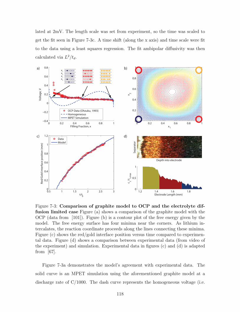
lated at 2mV. The length scale was set from experiment, so the time was scaled to

get the fit seen in Figure 7-3c. A time shift (along the x axis) and time scale were fit

to the data using a least squares regression. The fit ambipolar diffusivity was then

calculated via L2/td.

0 0.2 0.4 0.6 0.8 1−0.4

−0.2

0

0.2

0.4

0.6

0.8

Filling Fraction, x

Volta

ge, V

OCP Data (Ohzuku, 1993)HomogeneousMPET Simulation

x1x 2

0 0.2 0.4 0.6 0.8 10

0.2

0.4

0.6

0.8

1

0.5 1 1.5 2 2.5 30

0.2

0.4

0.6

0.8

1

1.2

t/t0

Red/

Gol

d in

terf

ace

posi

tion

(mm

)

DataModel


Sepa

rato

r

1.2 1.4 1.6 1.80

0.5

1

c s/cs,

max

Electrode Length (mm)

x1

x2x1x2

a) b)

c) d)

Figure 7-3: Comparison of graphite model to OCP and the electrolyte dif-fusion limited case Figure (a) shows a comparison of the graphite model with theOCP (data from [101]). Figure (b) is a contour plot of the free energy given by themodel. The free energy surface has four minima near the corners. As lithium in-tercalates, the reaction coordinate proceeds along the lines connecting these minima.Figure (c) shows the red/gold interface position versus time compared to experimen-tal data. Figure (d) shows a comparison between experimental data (from video ofthe experiment) and simulation. Experimental data in figures (c) and (d) is adaptedfrom [67].

Figure 7-3a demonstrates the model’s agreement with experimental data. The

solid curve is an MPET simulation using the aforementioned graphite model at a

discharge rate of C/1000. The dash curve represents the homogeneous voltage (i.e.

118

x1 = x2). The stress term given by Ωc causes this voltage to go negative and makes it

favorable for the particle layers to fill discretely. The inlay in Figure 7-3a shows the

representative graphite particles (i.e. the two layers used to represent graphite par-

ticles). The particles consist of alternating x1 and x2 layers. Close to empty, lithium

is randomly distributed throughout the layers. As lithium intercalates, the model

causes alternating layers to fill preferentially, producing the first voltage plateau.

Which layer fills (i.e. x1 or x2) is random, but has no effect on the voltage since both

states have the same chemical potential. After one layer fills, the other layer fills

preferentially, producing the second voltage plateau.

The free energy model defines three separate states in the particles (blue near

empty, red near half filling, and gold near full filling), however, it does not define

where this transition occurs. Somewhere past the first local minima, the transition

from blue to red occurs, and somewhere past the half filling state, the transition from

red to gold occurs. The model demonstrates a sharp solid concentration gradient

along the electrode between the half filling and filled states. We assume that around

0.6 (i.e. just past the half filling) the particles transition from red to gold. Given the

sharp gradient in solid particle concentration across the electrode, the choice of this

concentration does not have a large effect on the fit diffusivity.

The blue/red interface is more difficult to define, since real graphite has multiple

stages at low concentration. We assume the blue to red transition occurs around a

filling fraction of 0.3. This produces a good qualitative agreement with data, although

it is not required when the model is fit to the red/gold interface data and does not

affect the fit diffusivity. Coincidentally, the 0.3 filling fraction is located near the

beginning of the first plateau in the OCP data, which could be interpreted as the

beginning of the first phase represented in this model.

The contour plot in Figure 7-3b represents the free energy as the layers are filled.

The homogeneous state is penalized by a large free energy in the center of the contour

plot. There are four minima located near the corners corresponding to the empty,

half-full, and full states. As lithium intercalates, it starts near the blue circle (empty

state), then progresses towards one of minima inside the red circles (at random) then

119

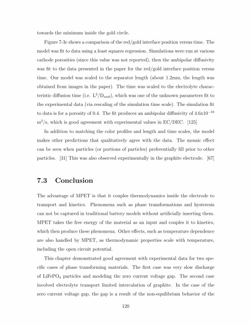
towards the minimum inside the gold circle.

Figure 7-3c shows a comparison of the red/gold interface position versus time. The

model was fit to data using a least squares regression. Simulations were run at various

cathode porosities (since this value was not reported), then the ambipolar diffusivity

was fit to the data presented in the paper for the red/gold interface position versus

time. Our model was scaled to the separator length (about 1.2mm, the length was

obtained from images in the paper). The time was scaled to the electrolyte charac-

teristic diffusion time (i.e. L2/Damb), which was one of the unknown parameters fit to

the experimental data (via rescaling of the simulation time scale). The simulation fit

to data is for a porosity of 0.4. The fit produces an ambipolar diffusivity of 4.6x10−10

m2/s, which is good agreement with experimental values in EC/DEC. [125]

In addition to matching the color profiles and length and time scales, the model

makes other predictions that qualitatively agree with the data. The mosaic effect

can be seen when particles (or portions of particles) preferentially fill prior to other

particles. [31] This was also observed experimentally in the graphite electrode. [67]

7.3 Conclusion

The advantage of MPET is that it couples thermodynamics inside the electrode to

transport and kinetics. Phenomena such as phase transformations and hysteresis

can not be captured in traditional battery models without artificially inserting them.

MPET takes the free energy of the material as an input and couples it to kinetics,

which then produce these phenomena. Other effects, such as temperature dependence

are also handled by MPET, as thermodynamic properties scale with temperature,

including the open circuit potential.

This chapter demonstrated good agreement with experimental data for two spe-

cific cases of phase transforming materials. The first case was very slow discharge

of LiFePO4 particles and modeling the zero current voltage gap. The second case

involved electrolyte transport limited intercalation of graphite. In the case of the

zero current voltage gap, the gap is a result of the non-equilibrium behavior of the

120

particles. At equilibrium, LiFePO4 phase separates, producing a voltage plateau.

However, during lithiation, particles can behave more homogeneously due to coher-

ent stress and current induced suppression of phase transformation. [45, 8] Surface

effects in the form of surface wetting can play a large role, as was shown in this paper.

These effects are responsible for the voltage gap being smaller than is predicted by

equilibrium thermodynamics of the particles.

In the second case, a new model for graphite was presented and fit to data with

great accuracy. In the graphite model, the free energy of the particles coupled to the

kinetics and transport in the electrolyte generates color profiles that match experi-

ment. These colors emerge as a result of the free energy model. In traditional battery

models, these effects would need to be artificially inserted into the model. More work

is needed on this new graphite free energy model to compare with other experiments

and test its validity when electrolyte transport is not limiting.

121

Chapter 8

Modeling Lithium Iron Phosphate

Electrodes

The recent work by Cogswell and Bazant investigating the effects of particle size,

surface wetting, and coherency strain on the lithiation dynamics of LiFePO4 (LFP)

particles represents an important step towards understanding the dynamics of the

material. [44] The model, which modeled plate-like nanoparticles in 2D with the

third dimension depth averaged, captured the source of the zero-current voltage gap

that was first observed and explained by Dreyer et al.. [54] Dreyer attributed this

zero-current voltage gap to particle-particle effects at the electrode scale using a non-

monotonic free energy model. Cogswell and Bazant expanded on this using phase

field modeling to explain why different voltage gaps were observed in different LFP

electrodes, and why the 20 mV observed in Dreyer’s work differs from the voltage gap

predicted by solid solution (i.e. homogeneous) thermodynamics.

In the previous chapter, a simplified form of this model was presented and fit

to the data of Dreyer et al.. [54] This is useful for very slow charge and discharge

models, since the particle-by-particle filling leads to large local current densities that

suppress any phase separation behavior. However, as the discharge rate is increased,

the number of active particles increases. This means the local current density of

the particles is smaller, and it might no longer be reasonable to assume that phase

separation dynamics are suppressed. Bai et al. demonstrated that the local current

123

density with respect to the exchange current density needs to be order one to suppress

phase separation. [8] Without simulations, it’s difficult to know exactly what these

local current densities are due to particle-particle interactions at the electrode scale.

This chapter represents the most recent work on modeling a LFP electrode. The

first part of this chapter will present the single particle model that will be used.

It is a simplified (i.e. 1D) version of Cogswell and Bazant’s 2D model. Once the

single particle model has been presented, a section on inserting it into the porous

electrode, and how to include different sized particles, will be presented. Finally,

some charge and discharge examples, along with comparison to experimental data

will be presented.

8.1 Single Particle Model

The complete model used by Cogswell and Bazant was in 2D, with the third dimen-

sion (the depth, or [010] direction) averaged. This model is quite computationally

expensive. Therefore, we wish to reduce the model to capture the same dynamics,

but make it less computationally expensive. Despite the full model being in 2D, the

overall dynamics of the system behave much like a 1D system, as the phase interface

propagates in the [100] direction across the surface. To simplify computation, we

model 1D particles. The particle shapes and sizes are the same as in Cogswell and

Bazant’s paper (also in the previous chapter). [44] The C3 shape particles are taken

from Smith et al.. [121] Once again, the thickness of the particles has to be assumed,

and a value of 20 nm is used. [121, 115]

To model the particles, the Cahn-Hilliard free energy functional, along with an

approximated coherency strain term are used. The chemical potential, based on this

free energy functional, is given by Equation 4.50. It is

µ = µ−∇ ·(κ

ρs∇c)

+B

ρs(c−X) . (8.1)

Values for ρs, κ, and B are taken from other work by Cogswell and Bazant. [45]

124

In this chapter, the dimensionless LFP concentration will be represented by c. The

value of B depends on the orientation of the interface as well as whether or not the

particles have coherent or semi-coherent strain. This model assumes semi-coherent

strain, since it is improbable that the particles are perfect crystals. The value of B in

the [100] direction for the case of semi-coherent strain, is almost the same as the [101]

direction in coherent strain. [45] Modeling phase separation in the [101] direction

requires the full 2D model. Interestingly enough, this semi-coherent 1D model should

have very similar effects from strain as the full 2D coherent case. The homogeneous

chemical potential, µ, is the regular solution model, and the value of Ω is also taken

from Cogswell and Bazant. [45]

One last effect that needs to be modeled in this system is the surface wetting

of the particles. In the full model, surface wetting is controlled by the boundary

condition, which dictates continuity of µ. Bazant referred to this as the “natural

boundary condition” and it is given by

∂γ

∂∇c= n · ∂g

∂∇c= n · κ∇c. (8.2)

One property of LFP is that the difference between the interfacial energies on the

facets is quite large, such that it’s probable that specific surfaces prefer to be com-

pletely wetted or de-wetted. [44] This means the boundary condition can be ap-

proximated using either a high concentration (near full) or a low concentration (near

empty) depending on the surface. Given the orientation of our 1D particles, the side

facets are treated as fully wetted (i.e. the dimensionless concentration is close to 1).

The top facet (the top [010] plane) should be de-wetted. However, this would increase

the computational complexity. For this model, the de-wetted top surface is neglected.

This surface could play an important role in the charge transfer reaction, though, so

depending on how well the model fits data and how reasonable the parameters are,

this effect may need to be added back into the model.

To simplify modeling the surface wetting, this model adds an additional volume

at the ends of the particles where lithium concentration is held constant. In these

125

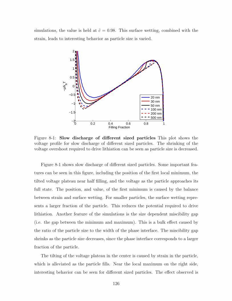
simulations, the value is held at c = 0.98. This surface wetting, combined with the

strain, leads to interesting behavior as particle size is varied.

0 0.2 0.4 0.6 0.8 1−2

−1.5

−1

−0.5

0

0.5

1

1.5

2

Filling Fraction

−µ/k

BT

20 nm30 nm50 nm100 nm200 nm500 nm

Figure 8-1: Slow discharge of different sized particles This plot shows thevoltage profile for slow discharge of different sized particles. The shrinking of thevoltage overshoot required to drive lithiation can be seen as particle size is decreased.

Figure 8-1 shows slow discharge of different sized particles. Some important fea-

tures can be seen in this figure, including the position of the first local minimum, the

tilted voltage plateau near half filling, and the voltage as the particle approaches its

full state. The position, and value, of the first minimum is caused by the balance

between strain and surface wetting. For smaller particles, the surface wetting repre-

sents a larger fraction of the particle. This reduces the potential required to drive

lithiation. Another feature of the simulations is the size dependent miscibility gap

(i.e. the gap between the minimum and maximum). This is a bulk effect caused by

the ratio of the particle size to the width of the phase interface. The miscibility gap

shrinks as the particle size decreases, since the phase interface corresponds to a larger

fraction of the particle.

The tilting of the voltage plateau in the center is caused by strain in the particle,

which is alleviated as the particle fills. Near the local maximum on the right side,

interesting behavior can be seen for different sized particles. The effect observed is

126

the result of the particle size dependence and the phase separated behavior. With

surface wetted nucleation, the lithium rich phases begin at the edges of the particles

and propagate towards the center. For smaller particles, this phase interface occupies

a larger fraction of the particle. Conversely, for larger particles, the phase interface

occupies a smaller portion of the particle. The width of the phase interface relative

to the particle size is important when the two phase interfaces collide and the particle

becomes homogeneous. For very small particles, the interfaces overlap and smoothly

fill, producing the smooth voltage curve. At intermediate sizes, there is a sharp voltage

spike associated with the interfaces colliding and filling quickly to a homogeneous

state. For very large particle sizes, this sharp voltage jump is reduced since the

volume that fills quickly is a very small fraction of the particle (i.e. its behavior does

not strongly affect the voltage curve).

This figure is very similar to Figure 4a in Cogswell and Bazant. [44] Despite the

reduction of the model (i.e. from 2D to 1D), the figures are similar because of the

properties of LiFePO4. Cogswell and Bazant demonstrated previously that coherent

strain leads to intercalation front propagation along the [101] direction. Furthermore,

imperfections in the crystal, leading to semi-coherent strain, lead to intercalation

front propagation in the [100] direction. [45] For this material, it just so happens

that the strain energies of the coherent and semi-coherent cases are approximately

the same. Therefore, the 1D case has very similar energetics to the 2D case. There

are slight differences, however, since the full 2D case, even with semi-coherent strain,

has effects from phase propagation along the [101] direction. For the purposes of

this simulation, though, this 1D model is a suitable representation of the LiFePO4

particles, as it demonstrates similar behavior and effects from particle size and surface

wetting.

127

8.2 Porous Electrode Modeling of Surface Wetted

LFP Particles with Coherency Strain

The overall goal is to use single particle models to gain insight into how porous

electrodes behave. Before that can be accomplished, though, the single particle model

must be inserted into a model for the porous electrode. Modified Porous Electrode

Theory (MPET), the focus of this thesis, is such a framework, as it couples all of the

effects inside the electrode to the thermodynamics of the system, including reaction

kinetics, transport, and the potential boundary condition. This section will deal with

incorporating the single particle model in the porous electrode, as well as how to

accurately represent a particle size distribution in a volume averaged system.

Inserting the ACR equation itself into the MPET framework is straightforward

based on the equations presented in this thesis. The chemical potential in Equation

8.1 can be used to calculate the activity. Transport in the electrolyte is handled via

the aforementioned mass conservation equations. One of the most important features

to add to the simulation is the particle size distribution. The size of the particles

affects the voltage profile as well as the distribution of current in the electrode.

In the previous chapter, where a size distribution was fit, the pseudocapacitor

model was used, which allowed concentration profiles inside the particles to be ne-

glected. This allowed for hundreds of particles to be modeled. In this model, though,

concentration profiles inside the particles need to be modeled with a resolution of at

least 1 nm in order to capture any phase interfaces. This corresponds to about a hun-

dred volumes per particle for particles on the order of 100 nm. Hundreds of particles

means there will be tens of thousands of solid volumes. This makes the system very

slow to simulate.

It’s advantageous to try to represent the electrode using as few particles as possi-

ble. This is problematic, though, because too few particles won’t accurately represent

the electrode, and too many particles will take a very long time to compute. Adding

a particle size distribution makes this more difficult. If particle sizes are chosen at

random, then a suitable number of particles needs to be added such that the size

128

distribution is accurately represented. Figure 8-2 represents a couple different ways

the particle size distribution can be added.

a) b)

Figure 8-2: Different schemes for addressing particle size distributions Thefigure denotes two possible methods to include particle size distributions. The schemeon the left uses a 2D grid with one particle size in each volume while the scheme onthe right uses a 1D grid with a particle size distribution inside each volume. Forfewer discretizations, the scheme on the right captures the active area better than thescheme on the left.

Figure 8-2a shows a 2D grid, with random sized particles inserted into each of

the volumes. If it is assumed that the volume of active material is roughly constant

throughout the volume, then this method assumes that the representative particles

are repeated inside the volume until the solid volume is reached. While this achieves

the proper active solid volume fraction, the area of the active particles is not well

represented. This is due to the surface to volume ratio of such small particles. Any

volume that contains small particles will require more particles to match the volume

of the active material, resulting in too large of an active area. Additionally, mass

and charge conservation in the vertical direction need to be accounted for, adding

computational complexity.

Figure 8-2b represents a suitable solution to this problem. Since transport in the

vertical direction does not often have strong concentration gradients (i.e. gradients

are predominantly along the horizontal axis, perpendicular to the separator), it makes

sense to reduce the model to 1D, but add a particle size distribution inside each of the

volumes. Each particle inside a respective volume is exposed to the same electrolyte

concentration and potential. This simplifies the computation a bit. Furthermore, the

129

area of the active material in the volume is more accurate, since a correct number

of large and small particles are represented. When scaling the simulation to the full

porous electrode, now each volume is repeated to match the total active volume. This

yields a better representation of the electrode.

8.3 Simulations

This section will present simulation results for the ACR model inside a porous elec-

trode. Three different discharge rates were selected: C/50, 1.5C, and 5C. The particle

concentration profiles are shown at filling fractions of 0.25 and 0.67 for each simu-

lation to highlight the differences in the electrode filling mechanisms. These filling

fractions were arbitrarily chosen.

The values selected here are chosen to highlight the particle-particle effects. A 50

µm electrode with a 25 µm separator was simulated. The electrode porosity was set

to 0.4 and the volume loading percent was 0.7. This porosity is larger than typical

batteries, and prevents electrolyte limitations at modest discharge rates (e.g. 5C).

The electrolyte was 1M LiPF6 in EC/DMC. [1] The particle size distribution was set

to an average particle size of 160 nm with a 20 nm standard deviation. Five volumes

inside the electrode were simulated (i.e. each volume is approximately 10 µm long)

with four representative particles in each volume. A charge transfer coefficient of 0.5

was used.

First, the C/50 discharge simulation is considered. Figure 8-3 shows the voltage

versus filling fraction and solid concentration profiles for the representative particles

throughout the electrode. The most noticeable effects in the voltage plot are the

small bumps observed towards the end of the discharge. These bumps are caused by

the discreteness of the model. With only 20 particles, single particle effects (namely

the non-monotonic voltage profile of a single particle) are observed as the number of

particles capable of sustaining the current approaches the single particle limit. In a

real electrode, this effect would not be observed since there are millions of particles.

Similarly, if millions of particles could be simulated, the effect would not be seen here

130

0 0.1 0.2 0.3 0.4 0.5 0.6 0.7 0.8 0.9 12.7

2.8

2.9

3

3.1

3.2

3.3

3.4

3.5

3.6

3.7

Filling Fraction

Volta

ge (V

)

0 219

0 177

0 188

0 139

0 151

0 155

0 182

0 155

0 175

0 119

0 153

0 144

0 129

0 171

0 166

0 161

0 134

0 183

0 168

0 155


Sepa

rato

r

Figure 8-3: C/50 discharge of ACR MPET model This figure shows solid con-centration profiles and a voltage versus filling fraction for C/50 discharge. The redand blue dots correspond to the colored solid concentration profiles.

either.

It’s difficult to see the method by which particles fill based on the provided figure.

Movies of the intercalation inside the particle show that the particles fill homoge-

neously, despite the phase separation being nucleated with surface wetting. This is

because the local current density is large enough to suppress phase separation. As

more representative particles are added to the simulation, the actual particle size

distribution is approached. For such slow discharge rates, the particles fill prefer-

entially from smallest to largest. This is a consequence of the surface wetting and

coherency strain in the particles, which leads to different overpotentials required to

drive lithiation. This model predicts that even with slow discharge the particles fill

homogeneously.

The red and blue dots denote the solid concentration profiles at different depths of

discharge. The red dot (which accompanies the red concentration profiles) is located

at a filling fraction of 0.25, while the blue dot (which matches the blue concentration

profiles) is located at a filling fraction of 0.67 (i.e. two thirds filling). The strong size

dependence can be seen in the concentration profiles, as the smaller particles fill first

followed by the larger particles. This is due to the size dependence from the surface

wetting and coherency strain, as demonstrated in Figure 8-1. Smaller particles require

131

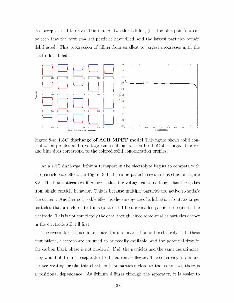
less overpotential to drive lithiation. At two thirds filling (i.e. the blue point), it can

be seen that the next smallest particles have filled, and the largest particles remain

delithiated. This progression of filling from smallest to largest progresses until the

electrode is filled.

0 0.1 0.2 0.3 0.4 0.5 0.6 0.7 0.8 0.9 12.7

2.8

2.9

3

3.1

3.2

3.3

3.4

3.5

3.6

3.7

Filling Fraction

Volta

ge (V

)

0 219

0 177

0 188

0 139

0 151

0 155

0 182

0 155

0 175

0 119

0 153

0 144

0 129

0 171

0 166

0 161

0 134

0 183

0 168

0 155


Sepa

rato

r

Figure 8-4: 1.5C discharge of ACR MPET model This figure shows solid con-centration profiles and a voltage versus filling fraction for 1.5C discharge. The redand blue dots correspond to the colored solid concentration profiles.

At a 1.5C discharge, lithium transport in the electrolyte begins to compete with

the particle size effect. In Figure 8-4, the same particle sizes are used as in Figure

8-3. The first noticeable difference is that the voltage curve no longer has the spikes

from single particle behavior. This is because multiple particles are active to satisfy

the current. Another noticeable effect is the emergence of a lithiation front, as larger

particles that are closer to the separator fill before smaller particles deeper in the

electrode. This is not completely the case, though, since some smaller particles deeper

in the electrode still fill first.

The reason for this is due to concentration polarization in the electrolyte. In these

simulations, electrons are assumed to be readily available, and the potential drop in

the carbon black phase is not modeled. If all the particles had the same capacitance,

they would fill from the separator to the current collector. The coherency strain and

surface wetting breaks this effect, but for particles close to the same size, there is

a positional dependence. As lithium diffuses through the separator, it is easier to

132

fill particles closer to the separator rather than particles deeper in the electrode (i.e.

closer to the current collector). This positional dependence becomes more pronounced

with faster discharge.

0 0.1 0.2 0.3 0.4 0.5 0.6 0.7 0.8 0.9 12.7

2.8

2.9

3

3.1

3.2

3.3

3.4

3.5

3.6

3.7

Filling FractionVo

ltage

(V)

0 219

0 177

0 188

0 139

0 151

0 155

0 182

0 155

0 175

0 119

0 153

0 144

0 129

0 171

0 166

0 161

0 134

0 183

0 168

0 155


Sepa

rato

r

Figure 8-5: 5C discharge of ACR MPET model This figure shows solid concen-tration profiles and a voltage versus filling fraction for 5C discharge. The red andblue dots correspond to the colored solid concentration profiles.

Figure 8-5 shows the discharge of the same electrode (i.e. the same particle sizes)

at 5C. The solid concentrations are very similar to the 1.5C discharge in Figure 8-4.

The main difference is in the voltage curve, though, which has been smoothed. This

is because the number of active particles has increased, reducing the fluctuations in

voltage associated with discrete filling in the electrode. Another difference is the end

of the voltage plateau, which shows a sweeping dropoff. This dropoff is caused by

variations in particle size. At constant current, as particles fill, fewer particles are

forced to sustain the same current, leading to increased overpotential. A particle

size distribution enhances this effect. Despite multiple particles being active, smaller

active particles still fill ahead of larger particles due to their smaller capacity. At the

end of the discharge, the current needs to be sustained by fewer particles. This leads

to increasing overpotential as particles “turn off”, leading to this sweeping dropoff

that has also been observed experimentally. [76]

Next, we look at how particles behave when charging. Figures 8-6 and 8-7 show

charging at C/50 and 1.5C rates. In Figure 8-6 the particles empty discretely and

133

0 0.1 0.2 0.3 0.4 0.5 0.6 0.7 0.8 0.9 12.7

2.8

2.9

3

3.1

3.2

3.3

3.4

3.5

3.6

3.7

Filling Fraction

Volta

ge (V

)

0 219

0 177

0 188

0 139

0 151

0 155

0 182

0 155

0 175

0 119

0 153

0 144

0 129

0 171

0 166

0 161

0 134

0 183

0 168

0 155


Sepa

rato

r

Figure 8-6: C/50 charge of ACR MPET model This figure shows solid concen-tration profiles and a voltage versus filling fraction for C/50 charge. The red and bluedots correspond to the colored solid concentration profiles.

based on size, as in the discharge example. Similarly, the bumps in the voltage plateau

denote the discrete emptying events. The dots denote the same filling fractions as

before, however, since the electrode is being charged, the red dot is reached first,

then the blue dot. All of the particles reach roughly the same concentration near

0.9, and then proceed to discretely empty. The voltage plateau is located above

3.42V standard potential, demonstrating that this model also captures the voltage

gap previously shown.

The more interesting behavior of charging is demonstrated when the charging rate

is increased. Figure 8-7 shows the results for a 1.5C charging rate. After an initial

climb in overpotential to drive the delithiation, all the particles reach a concentration

around 0.6 (note the end of the line in the voltage profile) after which the particles

discretely empty again, similar to the C/50 charging behavior. This behavior demon-

strates the difference between discharge and charge dynamics. The model predicts

that discharge at higher C-rates produce more homogeneous solid concentration pro-

files, whereas in charging, increasing the charging C-rate still produces some discrete

effects.

Next, some experimental results from Li and Chueh will be presented to show the

qualitative similarities between real electrodes and the ACR model presented in this

134

0 0.1 0.2 0.3 0.4 0.5 0.6 0.7 0.8 0.9 12.7

2.8

2.9

3

3.1

3.2

3.3

3.4

3.5

3.6

3.7

Filling Fraction

Volta

ge (V

)

0 219

0 177

0 188

0 139

0 151

0 155

0 182

0 155

0 175

0 119

0 153

0 144

0 129

0 171

0 166

0 161

0 134

0 183

0 168

0 155


Sepa

rato

r

Figure 8-7: 1.5C charge of ACR MPET model This figure shows solid concen-tration profiles and a voltage versus filling fraction for 1.5C charge. The red and bluedots correspond to the colored solid concentration profiles.

section.

8.3.1 Comparison to LFP Electrodes on Charge and Dis-

charge

The data presented here are from Li and Chueh. [43, 91] The figures are a combina-

tion of TEM images and X-ray absorption spectroscopy taken on slices of a partially

charged/discharged electrode (around half filling). The left image (TEM) denotes the

position of solid intercalation particles in the electrode (the black masses) and the

right image (X-ray absorption) denotes the filling fraction. The red sections are fully

lithiated, the green sections are delithiated, and the yellow sections are intermediate

concentrations. These yellow particles are considered to be “mixed”, and can contain

portions of red and green along with yellow. The number of mixed particles is what

will be compared to the model in this section.

Figure 8-8 shows the number of mixed particles for discharge rates of C/50, 1.5C,

and 5C. The C/50 and 1.5C discharge rates show that the number of mixed particles

is low. This is similar to the behavior predicted by the ACR model in this chapter

(near half filling). However, the model predicts more mixed particles for the 1.5C

135

a)

b)

c)

Figure 8-8: Electrode after discharge This figure shows the TEM and X-ray ab-sorption spectroscopy images for discharge rates of (a) C/50 (b) 1.5C and (c) 5C. Thecircles indicate the positions of “mixed” particles which are either homogeneous or amixture of full and empty portions, denoted by the yellow color. Figure courtesy ofLi and Chueh. [91]

136

discharge. The 5C figure shows that there is a large percentage of mixed particles,

which is similar to the behavior of the ACR model around half filling. The discrepancy

at medium discharge rates (i.e. around 1.5C) will be discussed later in this section.

Figure 8-9: Electrode after 1.5C charge This figure shows the TEM and X-rayabsorption spectroscopy images for a 1.5C charging rate. The circles indicate thepositions of “mixed” particles which are either homogeneous or a mixture of full andempty portions, denoted by the yellow color. Figure courtesy of Li and Chueh. [91]

Figure 8-9 shows particles after a 1.5C charge. Similar to the discharge figures, the

number of mixed particles is small. Other data from Li and Chueh (not shown here)

suggest that on charging, despite the charging rate, the number of mixed particles

remains much lower than on discharge. [91]

Given this experimental data, there are currently two discrepancies present be-

tween the model and the data. The first is that the number of mixed particles pre-

dicted by the model at intermediate discharge rates is too high. The 1.5C discharge

model shows many mixed particles around half filling, although the data does not.

The second discrepancy is that on charging, the model predicts that many particles

(almost the entire electrode) is close to the partially filled state. Figure 8-7 shows all

of the particles reach a filling fraction of approximately 0.6 prior to discretely emp-

tying. This is in contrast to the charging data which show a small number of mixed

particles.

In order to reconcile these differences, it’s important to consider the method used

in obtaining these images. The electrodes were prepared and then charged/dis-

charged. After the charge/discharge, the cell electrolyte was drained and replaced

137

with resin to keep the electrode in tact. However, there is an approximate 5 minute

relaxation time as the electrolyte is drained. To address this part of the experimental

procedure, a relaxation time (i.e. open circuit conditions, no net current) is added to

the end of the simulations.

Figures 8-10, 8-11, and 8-12 have the same format as the previous figures. The

profiles on the left represent the solid concentration profiles. Instead of a voltage

versus filling fraction figure, the right figure has been replaced with a voltage versus

time figure to denote the open circuit potential evolution as the electrode relaxes.

The voltage fluctuations are caused by charge transfer inside the electrode as lithium

shifts between particles and the electrolyte relaxes to its initial state (i.e. uniform

concentration).

0 50 100 150 200 250 3003.384

3.385

3.386

3.387

3.388

3.389

3.39

3.391

3.392

3.393

3.394

Time (s)

Volta

ge (V

)

0 219

0 177

0 188

0 139

0 151

0 155

0 182

0 155

0 175

0 119

0 153

0 144

0 129

0 171

0 166

0 161

0 134

0 183

0 168

0 155


Sepa

rato

r

Figure 8-10: Relaxation after 1.5 discharge of ACR MPET model This figureshows solid concentration profiles and a voltage versus time for relaxation after a1.5C discharge. The red and blue dots correspond to the colored solid concentrationprofiles at the beginning and end of the relaxation.

Figure 8-10 shows the concentration profiles after discharging at 1.5C to the half

filled state then letting the cell relax for 5 minutes. The red and blue dots (which

denote the potential at the different solid concentration profiles) are located at the

beginning and end points. In this figure, the voltage jumps quickly to about 3.389V

then slow relaxes towards the standard potential of 3.42V. This is because many of

the particles are closer to their equilibrium state when the current is turned off. At

138

the end of the relaxation, there is one particle in the half filled (i.e. the “mixed”)

state. The figure demonstrates how the particles relax and explains why so few

mixed particles are observed at 1.5C. Despite there being clusters of particles that

fill discretely, these particles relax to empty and filled states and not many particles

remain in the mixed state.

0 50 100 150 200 250 3003.38

3.39

3.4

3.41

3.42

3.43

3.44

3.45

Time (s)

Volta

ge (V

)

0 219

0 177

0 188

0 139

0 151

0 155

0 182

0 155

0 175

0 119

0 153

0 144

0 129

0 171

0 166

0 161

0 134

0 183

0 168

0 155


Sepa

rato

r

Figure 8-11: Relaxation after 5C discharge of ACR MPET model This figureshows solid concentration profiles and a voltage versus time for relaxation after a5C discharge. The red and blue dots correspond to the colored solid concentrationprofiles at the beginning and end of the relaxation.

Figure 8-11 demonstrates relaxation after a 5C discharge to a filling fraction of

0.5. This voltage curve shows a lot more activity since there are more active particles

near the half filled state when the current is turned off. To explain the kinetics of

the relaxation, we must refer to the single particle voltage profiles in Figure 8-1. The

phase separated and homogeneous voltage profiles are both non-monotonic. There

happens to be three points in the profile at the standard potential. The two on the

sides (i.e. near empty and full) are stable and the center point is meta-stable.

If the current is turned off, the model predicts that it may be possible for some

particles to be trapped near the half filled state (whether they are homogeneous or

phase separated). Although the voltage slopes upward (meaning the particle prefers

to have more lithium), this process is driven by delithiation of surrounding particles.

If nearest neighbors aren’t in a suitable state for lithium exchange, then extra time

139

is needed to communicate to other particles via the electrolyte.

It is because of this that many of the particles remain in the mixed state even

after relaxation. Particles closer to the minimum/maximum open circuit potential

solid concentrations have a higher driving force to relax to the zero chemical potential

state, either by lithiation or delithiation. Particles closer to the half filled state

have a smaller driving force (i.e. overpotential) relative to other particles near the

spinodal concentrations (i.e. the concentrations that correspond to the minimum and

maximum potentials). Therefore even after relaxation, they could become “stuck” at

this point, and take a long time to relax back to their empty or filled state.

It is important to note that the C/50 relaxation has been omitted here. This is

because the relaxation shows little to no change in solid concentration. Because of

how the particles fill, that is, discretely and nearly one-by-one, there is almost never

a time in the system where large numbers of particles are largely out of equilibrium.

When the current is turned off, the particles, which are already close to the stable

points (full or empty) relax quickly, and no changes are observed.

These two figures show, qualitatively, why intermediate discharge rates such as

1.5C show so few mixed particles, and why faster discharge rates show so many mixed

particles. A prediction from the model is that at even higher rates, the number of

mixed particles (for the same ending filling fraction and relaxation time) will be the

same. This has to do with how many of the particles in the electrode are active.

Finally, the discrepancy on charging will be addressed.

Figure 8-12 shows the relaxation after a 1.5C charging to a filling fraction of 0.5.

At the beginning of the relaxation, many of the particles are close to the half filled

state. This was seen in Figure 8-7 as well, at the end of the sloping line. However,

when the particles are relaxed, the active particles quickly relax and the particles

near the half filling state deeper in the electrode lithiate back to near full states.

This relaxation shows how despite there being many mixed particles, the relaxation

process can reduce the number of mixed particles after charging.

The asymmetry between the number of mixed particles on charge and discharge

is very interesting in the experiment. In the model, this is a consequence of the

140

0 50 100 150 200 250 3003.41

3.415

3.42

3.425

3.43

3.435

3.44

3.445

3.45

3.455

3.46

Time (s)

Volta

ge (V

)

0 219

0 177

0 188

0 139

0 151

0 155

0 182

0 155

0 175

0 119

0 153

0 144

0 129

0 171

0 166

0 161

0 134

0 183

0 168

0 155


Sepa

rato

r

Figure 8-12: Relaxation after 1.5C charge of ACR MPET model This figureshows solid concentration profiles and a voltage versus time for relaxation after a 1.5Ccharge. The red and blue dots correspond to the colored solid concentration profilesat the beginning and end of the relaxation.

exchange current density model used, which includes the enthalpic effects from the

regular solution model in the reductant activity. This enthalpic interaction skews the

exchange current density, making it asymmetric and giving it a maximum near the

lower concentration spinodal point. This term indicates that lithiation could be easier

than delithiation, and that delithiation may require a larger overpotential, as shown

in the charging simulations.

This term was naively included in some of the earliest forms of LFP models done

by our group. [120, 33, 8] However, more work is needed to determine the accuracy

of this term and whether it is accurate for the kinetics. An additional effect not

included in the model is the de-wetting of the active surface. [44] Although the

side facets are wetted and can nucleated the phase separation, the top facet, through

which intercalation actually occurs is energetically favored to be de-wetted. This

could affect the kinetics on charge and discharge, making charging more difficult

since lithium needs to be brought to the de-wetted surface before it can undergo a

charge transfer reaction to leave the particle.

141

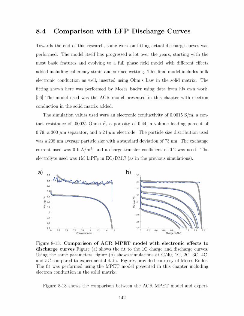
8.4 Comparison with LFP Discharge Curves

Towards the end of this research, some work on fitting actual discharge curves was

performed. The model itself has progressed a lot over the years, starting with the

most basic features and evolving to a full phase field model with different effects

added including coherency strain and surface wetting. This final model includes bulk

electronic conduction as well, inserted using Ohm’s Law in the solid matrix. The

fitting shown here was performed by Moses Ender using data from his own work.

[56] The model used was the ACR model presented in this chapter with electron

conduction in the solid matrix added.

The simulation values used were an electronic conductivity of 0.0015 S/m, a con-

tact resistance of .00025 Ohm·m2, a porosity of 0.44, a volume loading percent of

0.79, a 300 µm separator, and a 24 µm electrode. The particle size distribution used

was a 208 nm average particle size with a standard deviation of 73 nm. The exchange

current used was 0.1 A/m2, and a charge transfer coefficient of 0.2 was used. The

electrolyte used was 1M LiPF6 in EC/DMC (as in the previous simulations).

0 0.2 0.4 0.6 0.8 1 1.2 1.4 1.62.7

2.8

2.9

3

3.1

3.2

3.3

3.4

3.5

Charge (mAhr)

Volta

ge (V

)

0 0.2 0.4 0.6 0.8 1 1.2 1.4 1.62.7

2.8

2.9

3

3.1

3.2

3.3

3.4

3.5

3.6

3.7

Charge (mAhr)

Volta

ge (V

)

a) b)

Figure 8-13: Comparison of ACR MPET model with electronic effects todischarge curves Figure (a) shows the fit to the 1C charge and discharge curves.Using the same parameters, figure (b) shows simulations at C/40, 1C, 2C, 3C, 4C,and 5C compared to experimental data. Figures provided courtesy of Moses Ender.The fit was performed using the MPET model presented in this chapter includingelectron conduction in the solid matrix.

Figure 8-13 shows the comparison between the ACR MPET model and experi-

142

mental discharge curves. The figure in 8-13a shows the initial fit to 1C charge and

discharge curves. The initial fit captures the data very well. The 1C charging curve

has some strong oscillations due to the discreteness of the model, but seems to capture

the overall effects and the experimental data follows the average of the simulation val-

ues. In Figure 8-13b, the model captures the initial voltage for each of the discharge

rates quite well. However, the model does not accurately predict the capacity of the

cell.

The parameters used in this simulation were predominantly taken from experi-

mental measurements and analysis of the microstructure. This is promising since the

number of fitted parameters was small. However, the conductivity of the solid phase

used is orders of magnitude smaller than that predicted by microstructure analysis.

Given such a large difference, it’s possible that effects are missing from the model,

such as electron conduction in the poorly conducting LFP particles.

Despite not accurately capturing all the data, this fit shows that the model is

proceeding in the correct direction. As this work continues and more effects are

added to the model, fitting of voltage curves should improve.

8.5 Conclusion

This chapter highlights the most recent work using MPET. While showing great

qualitative and even quantitative agreement with data, it still shows that there is

work to do to accurately model LFP. One of the main areas that needs focus is

the single particle modeling. A full 3D single particle model that addresses coherency

strain as well as surface wetting is needed to better understand the active and inactive

facets during lithiation and delithiation. Using this information, important effects can

be included into the porous electrode model.

Another potentially important feature of LFP that needs to be researched is elec-

tron conduction. LFP is a poor electron conductor, which is why carbon coated

LFP particles perform so much better than non-coated particles. [113] These coat-

ings aren’t necessarily uniform, though, and more research on the effect of electron

143

conduction in the surfaces needs to be done.

A third area of research for LFP is the reaction rate. The reaction rate used in

MPET, which is a self consistent formulation, is dependent on understanding the

material as well as how the reaction proceeds (namely the transition state). To date,

not much is understood about the charge transfer kinetics of LFP, including the energy

of the transition state. Additionally, it is unknown if there are any rearrangement

energies that require Marcus theory to address [94], which could also affect the

charge transfer coefficient. As research continues, these questions will be answered

and provide better insight into how lithiation occurs in LFP and potentially how it

can be improved even further.

144

Chapter 9

Conclusion

The overall goal of this thesis was to build a thermodynamically self-consistent frame-

work for modeling lithium-ion batteries. The motivation for this is phase separating

materials, which previously required artificial insertion of phase interfaces and other

effects. Modified Porous Electrode Theory accomplishes this goal. It provides a con-

sistent approach to modeling lithium transport in the electrolyte, the solid, as well

as a consistent approach to modeling the open circuit potential and charge transfer

kinetics. However, this isn’t the end of this research. In fact, it has only just begun.

In our quest to create this framework, we have included additional energetic ef-

fects inside our intercalation materials that tend to yield more questions than answers.

More complicated effects, such as surface wetting and coherency strain in LiFePO4,

are required to explain the complicated dynamics, and this is only material. Many

other battery materials demonstrate different phenomena including phase transforma-

tions over a narrow range of lithium concentrations, multiple phase transformations

(as demonstrated for graphite), and zero coherency strain. The MPET framework

provides the necessary equations to simulate discharge of these complicated materials,

however, a thorough understanding of the material itself, including various material

property energies, is required first. Once these things are known, though, MPET has

the ability to not only capture complicated dynamics, but also predict non-equilibrium

dynamics of the material.

This thesis work has demonstrated the ability of the model to explain the voltage

145

gap in LFP, capture multiple phase separations in graphite, and qualitatively ex-

plain charge and discharge lithiation in an LFP electrode. As the research progresses,

the understanding of these materials will improve, enabling researchers to build bet-

ter performing batteries by exploiting particle properties as well as particle-particle

interactions.

146

Bibliography

[1] Handbook of Battery Materials. Wiley, 2 edition, 2011.

[2] S.M. Allen and J.W. Cahn. Microscopic theory for antiphase boundary motion

and its application to antiphase domain coarsening. Acta Metallurgica, 27:1085–

1095, 1979.

[3] Pankaj Arora, Marc Doyle, Antoni S. Gozdz, Ralph E. White, and John New-

man. Comparison between computer simulations and experimental data for

high-rate discharges of plastic lithium-ion batteries. Journal of Power Sources,

88:219–231, 2000.

[4] Uri M. Ascher and Linda R. Petzold. Computer methods for ordinary differential

equations and differential-algebraic equations. Society for Industrial and Applied

Mathematics, 1998.

[5] H. Assadi. Phase-field modelling of electro-deoxidation in molten salt. Modelling

and Simulation in Materials Science and Engineering, 14:963–974, 2006.

[6] S. Atlung, K. West, and T. Jacobsen. Dynamic aspects of solid solution cath-

odes for electrochemical power sources. Journal of the Electrochemical Society,

126(8), 1979.

[7] Ali Awarkea, Sven Lauerb, Stefan Pischingera, and Michael Wittlera.

Percolation-tunneling modeling for the study of the electric conductivity in

LiFePO4 based li-ion battery cathodes. Journal of Power Sources, 196:405–

411, 2011.

147

[8] Peng Bai, Daniel Cogswell, and Martin Z. Bazant. Suppression of phase sep-

aration in LiFePO4 nanoparticles during battery discharge. Nano Letters,

11(11):4890–4896, 2011.

[9] N. Balke, S. Jesse, A. N. Morozovska, E. Eliseev, D. W. Chung, Y. Kim,

L. Adamczyk, R. E. Garca, N. Dudney, and S. V. Kalinin. Nanoscale map-

ping of ion diffusion in a lithium-ion battery cathode. Nature Nanotechnology,

5, 2010.

[10] Robert W. Balluffi, Samuel M. Allen, and W. Craig Carter. Kinetics of mate-

rials. Wiley, 2005.

[11] M. Z. Bazant. Mathematical Modeling of Electrochemical Energy Systems. Mas-

sachusetts Institute of Technology, 2009. lecture notes for subject 10.95.

[12] M. Z. Bazant. 10.626 Electrochemical Energy Systems. Massachusetts Institute

of Technology: MIT OpenCourseWare, http://ocw.mit.edu, License: Creative

Commons BY-NC-SA, 2011.

[13] M. Z. Bazant. Theory of chemical kinetics and charge transfer based on non-

equilibrium thermodynamics. Accounts of Chemical Research, 46:1144–1160,

2013.

[14] M. Z. Bazant, K. T. Chu, and B. J. Bayly. Current-voltage relations for elec-

trochemical thin films. SIAM Journal on Applied Mathematics, 65:1463–1484,

2005.

[15] M. Z. Bazant, M. S. Kilic, B. D. Storey, and A. Ajdari. Nonlinear electrokinetics

at large voltages. New Journal of Physics, 11:075016, 2009.

[16] M. Z. Bazant, M. S. Kilic, B.D. Storey, and A. Ajdari. Towards an under-

standing of nonlinear electrokinetics at large voltages in concentrated solutions.

Advances in Colloid and Interface Science, 152:48–88, 2009.

148

[17] M. Z. Bazant, B. D. Storey, and A. A. Kornyshev. Double layer in ionic liquids:

Overscreening versus crowding. Physical Review Letters, 106:046102, 2011.

[18] M. Z. Bazant, K. Thornton, and A. Ajdari. Diffuse charge dynamics in electro-

chemical systems. Physical Review E, 70:021506, 2004.

[19] P. M. Biesheuvel, A. A. Franco, and M. Z. Bazant. Diffuse-charge effects in

fuel-cell membranes. Journal of the Electrochemical Society, 156:B225–B233,

2009.

[20] P. M. Biesheuvel and J. Lyklema. Sedimentation–diffusion equilibrium of bi-

nary mixtures of charged colloids including volume effects. Journal of Physics:

Condensed Matter, 17:6337, 2005.

[21] P. M. Biesheuvel and M. van Soestbergen. Counterion volume effects in mixed

electrical double layers. Journal of Colloid and Interface Science, 316:490–499,

2007.

[22] P.M. Biesheuvel and M.Z. Bazant. Nonlinear dynamics of capacitive charging

and desalination by porous electrodes. Physical Review E, 81, 2010.

[23] P.M. Biesheuvel, Y. Fu, and M.Z. Bazant. Diffuse charge and faradaic reactions

in porous electrodes. Physical Review E, 83, 2011.

[24] P.M. Biesheuvel, Y. Fu, and M.Z. Bazant. Electrochemistry and capacitive

charging of porous electrodes in asymmetric multicomponent electrolytes. Rus-

sian Journal of Electrochemistry, 2012.

[25] P.M. Biesheuvel, R. Zhao, S. Porada, and A. van der Wal. Theory of membrane

capacitive deionization including the effect of the electrode pore space. Journal

of Colloid and Interface Science, 360:239–248, 2011.

[26] W.J. Boettinger, S.R. Coriell, A.L. Greer, A. Karma, W. Kurz, M. Rappaz,

and R. Trivedi. Solidification microstructures: Recent developments, future

directions. Acta Materialia, 48:43–70, 2000.

149

[27] W.J. Boettinger and J.A. Warren. The phase-field method: Simulation of alloy

dendritic solidification during recalescence. Metallurgical and Materials Trans-

actions A, 27:657–669, 1996.

[28] W.J. Boettinger, J.A. Warren, C. Beckermann, and A. Karma. Phase-field

simulation of solidification. Annual Review of Materials Research, 32:163–194,

2002.

[29] A. Bonnefont, F. Argoul, and M.Z. Bazant. Analysis of diffuse-layer effects

on time-dependent interfacial kinetics. Journal of Electroanalytical Chemistry,

500:52–61, 2001.

[30] D.A.G. Bruggeman. Berechnung verschiedener physikalischer konstanten von

heterogenen substanzen. Annalen der Physik, 1935.

[31] Damian Burch. Intercalation Dynamics in Lithium-Ion Batteries. Ph.D. Thesis

in Mathematics, Massachusetts Institute of Technology, 2009.

[32] Damian Burch and Martin Z. Bazant. Size-dependent spinodal and miscibility

gaps for intercalation in nanoparticles. Nano Letters, 9(11):3795–3800, 2009.

[33] Damian Burch, Gogi Singh, Gerbrand Ceder, and Martin Z. Bazant. Phase-

transformation wave dynamics LiFePO4. Solid State Phenomena, 139:95–100,

2008.

[34] J. W. Cahn and J. W. Hilliard. Free energy of a non-uniform system: I. inter-

facial energy. Journal of Chemical Physics, 28:258–267, 1958.

[35] John Cahn. Free energy of a nonuniform system. ii. thermodynamic basis.

Journal of Chemical Physics, 30(5):1121–1124, 1959.

[36] John Cahn. On spinodal decomposition. Acta Metallurgica, 9(9):795–801, 1961.

[37] John Cahn. Coherent fluctuations and nucleation in isotropic solids. Acta

Metallurgica, 10, 1962.

150

[38] John Cahn. On spinodal decomposition in cubic crystals. Acta Metallurgica,

10, 1962.

[39] John Cahn and John Hilliard. Free energy of a nonuniform system. iii. nucle-

ation in a two-component incompressible fluid. Journal of Chemical Physics,

31(3):688–699, 1959.

[40] G. Ceder, Y.-M. Chiang, D.R. Sadoway, M.K. Aydinol, Y.-I. Jang, and

B. Huang. Identification of cathode materials for lithium batteries guided by

first-principles calculations. Nature, 392:694–696, 1998.

[41] Guoying Chen, Xiangyun Song, and Thomas Richardson. Electron microscopy

study of the LiFePO4 to FePO4 phase transition. Electrochemical and Solid

State Letters, 9(6):A295–A298, 2006.

[42] L. Q. Chen. Phase-field models for microstructural evolution. Annual Review

of Materials Research, 32:113–140, 2002.

[43] William C Chueh, Farid El Gabaly, Josh D Sugar, Norman C. Bartelt, An-

thony H. McDaniel, Kyle R Fenton, Kevin R. Zavadil, Tolek Tyliszczak, Wei

Lai, and Kevin F. McCarty. Intercalation pathway in many-particle LiFePO4

electrode revealed by nanoscale state-of-charge mapping. Nano Letters, 13:866

– 872, 2013.

[44] D. A. Cogswell and M. Z. Bazant. Theory of coherent nucleation in phase-

separating nanoparticles. Nano Letters, Article ASAP, 2013.

[45] Daniel A. Cogswell and Martin Z. Bazant. Coherency strain and the kinetics

of phase separation in LiFePO4 nanoparticles. ACS Nano, 6:2215–2225, 2012.

[46] S. Dargaville and T.W. Farrell. Predicting active material utilization in LiFePO4

electrodes using a multiscale mathematical model. Journal of the Electrochem-

ical Society, 157(7):A830–A840, 2010.

151

[47] R. de Levie. On porous electrodes in electrolyte solutions. Electrochimica Acta,

8:751–780, 1963.

[48] R. de Levie. On porous electrodes in electrolyte solutions - iv. Electrochimica

Acta, 9:1231–1245, 1964.

[49] C. Delmas, M. Maccario, L. Croguennec, F. Le Cras, and F. Weill. Lithium

deintercalation of LiFePO4 nanoparticles via a domino-cascade model. Nature

Materials, 7:665–671, 2008.

[50] Pauline DeVidts and Ralph E. White. Governing equations for transport in

porous electrodes. Journal of the Electrochemical Society, 144(4), 1997.

[51] Marc Doyle, Thomas F. Fuller, and John Newman. Modeling of galvanostatic

charge and discharge of the lithium/polymer/insertion cell. Journal of the Elec-

trochemical Society, 140(6):1526–1533, 1993.

[52] Marc Doyle, Antoni S. Gozdz, Caroline N. Schmuts, Jean-Marie Tarascon, and

John Newman. Comparison of modeling predictions with experimental data

from plastic lithium ion cells. Journal of the Electrochemical Society, 143(6),

1996.

[53] D. Dreyer, C. Guhlke, and R. Huth. The behavior of a many-particle electrode

in a lithium-ion battery. Physica D, 240:1008–1019, 2011.

[54] Wolfgang Dreyer, Janko Jamnik, Clemens Guhlke, Robert Huth, Joze Moskon,

and Miran Gaberscek. The thermodynamic origin of hysteresis in insertion

batteries. Nature Materials, 9:448–453, 2010.

[55] M. Eikerling, A. A. Kornyshev, and E. Lust. Optimized structured of

nanoporous carbonbased double-layer capacitors. Journal of the Electrochemical

Society, 152:E24, 2005.

[56] Moses Ender, Todd R. Ferguson, Raymond B. Smith, and Martin Z. Bazant.

In preparation, 2013.

152

[57] J. Euler and W. Nonnenmacher. Current distribution in porous electrodes.

Electrochimica Acta, 2:268–286, 1960.

[58] T. R. Ferguson and M. Z. Bazant. Non-equilibrium thermodynamics of porous

electrodes. Journal of the Electrochemical Society, 159:A1967–A1985, 2012.

[59] Thomas Fuller, Marc Doyle, and John Newman. Simulation and optimization

of the dual lithium ion insertion cell. Journal of the Electrochemical Society,

141(1):1–10, 1994.

[60] R. Edwin Garcia and Yet-Ming Chiang. Spatially resolved modeling of mi-

crostructurally complex battery architectures. Journal of the Electrochemical

Society, 154(9):A856–A864, 2007.

[61] R. Edwin Garcia, Yet-Ming Chiang, W. Craig Carter, Pimpa Limthongkul,

and Catherine M. Bishop. Microstructural modeling and design of recharge-

able lithium-ion batteries. Journal of the Electrochemical Society, 152(1):A255–

A263, 2005.

[62] S. R. De Groot and P. Mazur. Non-equilibrium Thermodynamics. Interscience

Publishers, Inc., New York, NY, 1962.

[63] I.G. Gurevich and V.S. Bagotzky. Steady-state operation of a porous electrode

polarized from one side with diffusion supply of liquid reactants from both sides.

Electrochimica Acta, 12:593–614, 1967.

[64] J. E. Guyer, W. J. Boettinger, J. A. Warren, and G. B. McFadden. Phase field

modeling of electrochemistry i: Equilibrium. Physical Review E, 69:021603,

2004.

[65] J. E. Guyer, W. J. Boettinger, J. A. Warren, and G. B. McFadden. Phase field

modeling of electrochemistry ii: Kinetics. Physical Review E, 69:021604, 2004.

[66] B.C. Han, A. Van der Ven, D. Morgan, and G. Ceder. Electrochemical modeling

of intercalation processes with phase field models. Electrochimica Acta, 49:4691–

4699, 2004.

153

[67] Stephen J. Harris, Adam Timmons, Daniel R. Baker, and Charles Monroe.

Direct in situ measurements of li transport in li-ion battery negative electrodes.

Chemical Physics Letters, 485:265–274, 2010. Video of experiment available at

http://lithiumbatteryresearch.com/.

[68] Kuei-Feng Hsu, Sun-Yuan Tsay, and Bing-Joe Hwang. Synthesis and character-

ization of nano-sized LiFePO4 cathode materials prepared by a citric acid-based

sol-gel route. Journal of Materials Chemistry, 14:2690–2695, 2004.

[69] H. Huang, S.C.Yin, and L.F. Nazar. Approaching theoretical capacity of

LiFePO4 at room temperature at high rates. Electrochemical and Solid State

Letters, 4(10):A170–A172, 2001.

[70] R. A. Huggins. Advanced Batteries: Materials Science Aspects. Springer, 2009.

[71] E.A. Grens II. On the assumptions underlying theoretical models for flooded

porous electrodes. Electrochimica Acta, 15:1047–1057, 1970.

[72] E.A. Grens II and C.W. Tobias. The influence of electrode reaction kinetics on

the polarization of flooded porous electrodes. Electrochimica Acta, 10:761–772,

1965.

[73] E. M. Itskovich, A. A. Kornyshev, and M. A. Vorotyntsev. Electric current

across the metal-solid electrolyte interface. i. direct current, current-voltage

characteristic. Physica Status Solidi (a), 39:229–238, 1977.

[74] J. Jamnik and J. Maier. Generalised equivalent circuits for mass and charge

transport : chemical capacitance and its implications. Physical Chemistry

Chemical Physics, 3:1668–1678, 2001.

[75] A. M. Johnson and John Newman. Desalting by means of porous carbon elec-

trodes. Journal of the Electrochemical Society, 118:510–517, 1971.

[76] Byoungwoo Kang and Gerbrand Ceder. Battery materials for ultrafast charging

and discharging. Nature, 458:190–193, 2009.

154

http://lithiumbatteryresearch.com/

[77] A. Karma. Phase-field model of eutectic growth. Physical Review E, 49:2245–

2250, 1994.

[78] Dirk Kehrwald, Paul R. Shearing, Nigel P. Brandon, Puneet K. Sinha, and

Stephen J. Harris. Local tortuosity inhomogeneities in a lithium battery com-

posite electrode. Journal of the Electrochemical Society, 158(12):A1393–A1399,

2011.

[79] M. S. Kilic, M. Z. Bazant, and A. Ajdari. Steric effects in the dynamics of

electrolytes at large applied voltages: I double-layer charging. Physical Review

E, 75:021502, 2007.

[80] M. S. Kilic, M. Z. Bazant, and A. Ajdari. Steric effects on the dynamics of elec-

trolytes at large applied voltages: II modified nernst-planck equations. Physical

Review E, 75:021503, 2007.

[81] A. A. Kornyshev and M. A. Vorotyntsev. Conductivity and space charge phe-

nomena in solid electrolytes with one mobile charge carrier species, a review

with original material. Electrochimica Acta, 26:303–323, 1981.

[82] O.S. Ksenzhek. Macrokinetics of processes on porous electrodes. Electrochimica

Acta, 9:629–637, 1964.

[83] O.S. Ksenzhek and V.V. Stender. Doklady Akademiia nauk SSSR, 106:486,

1956.

[84] O.S. Ksenzhek and V.V. Stender. Doklady Akademiia nauk SSSR, 107:280,

1956.

[85] O.S. Ksenzhek and V.V. Stender. Zhurnal prikladnoi khimii, 32:110, 1959.

[86] Karthikeyan Kumaresan, Yuriy Mikhaylik, and Ralph E. White. A mathemat-

ical model for a lithium-sulfur cell. Journal of The Electrochemical Society,

155:A576–A582, 2008.

155

[87] W. Lai and F. Ciucci. Thermodynamics and kinetics of phase transformation

in intercalation battery electrodes - phenomenological modeling. Electrochimica

Acta, 56:531–542, 2010.

[88] W. Lai and S. M. Haile. Impedance spectroscopy as a tool for chemical and

electrochemical analysis of mixed conductors: A case study of ceria. Journal of

the American Ceramic Society, 88:2979–2997, 2005.

[89] Wei Lai. Electrochemical modeling of single particle intercalation battery mate-

rials with different thermodynamics. Journal of Power Sources, 196:6534–6553,

2011.

[90] Wei Lai and Francesco Ciucci. Mathematical modeling of porous battery elec-

trodes - revisit of newman’s model. Electrochimica Acta, 56:4369–4377, 2011.

[91] Yiyang Li, Todd R. Ferguson, Raymond B. Smith, Martin Z. Bazant, and

William Chueh. In preparation, 2013.

[92] Rahul Malik, Damian Burch, Martin Bazant, and Gerbrand Ceder. Particle

size dependence of the ionic diffusivity. Nano Letters, 10:4123–4127, 2010.

[93] Rahul Malik, Fei Zhou, and Gerbrand Ceder. Kinetics of non-equilibrium

lithium incorporation in LiFePO4. Nature Materials, 10:587–590, 2011.

[94] R. A. Marcus. Electron transfer reactions in chemistry. theory and experiment.

Reviews of Modern Physics, 65:599–610, 1993.

[95] Graeme Walter Milton. The Theory of Composites. Cambridge University Press,

2002.

[96] D. Morgan, A. Van der Ven, and G. Ceder. Li conductivity in LixMPO4

(m=mn,fe,co,ni) olivine materials. Electrochemical and Solid State Letters,

7(2):A30–A32, 2004.

[97] E. Bruce Nauman and D. Qiwei Heb. Nonlinear diffusion and phase separation.

Chemical Engineering Science, 56:1999–2018, 2001.

156

[98] John Newman and Karen E. Thomas-Alyea. Electrochemical Systems. Prentice-

Hall, Inc., Englewood Cliffs, NJ, third edition, 2004.

[99] John Newman and William Tiedemann. Porous-electrode theory with battery

applications. AIChE Journal, 21(1):25–41, 1975.

[100] John Newman and Charles Tobias. Theoretical analysis of current distribution

in porous electrodes. Journal of The Electrochemical Society, 109(12):1183–

1191, 1962.

[101] Tsutomu Ohzuku, Yasunobu Iwakoshi, and Keijiro Sawai. Formation of lithium-

graphite intercalation compounds in nonaqueous electrolytes and their applica-

tion as a negative electrode for a lithium ion (shuttlecock) cell. Journal of the

Electrochemical Society, 140:2490–2498, 1993.

[102] L. H. Olesen, M. Z. Bazant, and H. Bruus. Strongly nonlinear dynamics of

electrolytes in large ac voltages. Physical Review E, 82:011501, 2010.

[103] Gosuke Oyama, Yuki Yamada, Ryuichi Natsui, Shinichi Nishimura, and At-

suo Yamada. Kinetics of nucleation and growth in two-phase electrochemical

reaction of LiFePO4. The Journal of Physical Chemistry C, 116:7306–7311,

2012.

[104] A.K. Padhi, K.S. Nanjundaswamy, and J.B. Goodenough. Phospho-olivines as

positive-electrode materials for rechargeable lithium batteries. Journal of the

Electrochemical Society, 144(4):1188–1194, 1997.

[105] Mauro Pasquali, Alessandro DellEra, and Pier Paolo Prosini. Fitting of the

voltage-li+ insertion curve of LiFePO4. Journal of Solid State Electrochemistry,

13:1859–1865, 2009.

[106] E. E. Petersen. Diffusion in a pore of varying cross section. AIChE Journal,

4:343–345, 1958.

157

[107] R. Pollard and J. Newman. Transient behavior of porous electrodes with high

exchange current densities. Electrochimica Acta, 25:315–321, 1980.

[108] W. Pongsaksawad, A. C. Powell, and D. Dussault. Phase-field modeling of

transport-limited electrolysis in solid and liquid states. Journal of The Electro-

chemical Society, pages F122–F133, 2007.

[109] S. Porada, L. Weinstein, R. Dash, A. van der Wal, M. Bryjak, Y. Gogotsi,

and P.M. Biesheuvel. Water desalination using capacitive deionization with

microporous carbon electrodes. ACS Applied Materials and Interfaces, 4:1194–

1199, 2012.

[110] David V. Ragone. Thermodynamics of Materials: Volume 1. John Wiley and

Sons, Inc., 1995.

[111] Venkatasailanathan Ramadesigan, Paul W. C. Northrop, Sumitava De, Shriram

Santhanagopalan, Richard D. Braatz, and Venkat R. Subramanian. Modeling

and simulation of lithium-ion batteries from a systems engineering perspective.

Journal of The Electrochemical Society, 159:R31–R45, 2012.

[112] S.K. Rangarajan. Theory of flooded porous electrodes. Electroanalytical Chem-

istry and Interfacial Electrochemistry, 22:89–104, 1969.

[113] N. Ravet, Y. Chouinard, J.F. Morgan, S. Besner, M. Gauthier, and M. Armand.

Electroactivity of natural and synthetic triphylite. Journal of Power Sources,

97-98:503–507, 2001.

[114] Muhammad Sahimi. Heterogeneous Materials I Linear Transport and Optical

Properties, volume 22 of Interdisciplinary Applied Mathematics. Springer, 2003.

[115] Kuppan Saravanan, Palani Balaya, M.V. Reddy, B.V.R Chowdar, and Ja-

gadese J. Vittal. Morphology controlled sythesis of lifepo4/c nanoplates for

li-ion batteries. Energy and Environmental Science, 3:457–464, 2010.

158

[116] Lawrence F. Shampine and Mark W. Reichelt. The matlab ode suite. SIAM

Journal on Scientific Computing, 18(1):1–22, 1997.

[117] Lihua Shen and Zhangxin Chen. Critical review of the impact of tortuosity on

diffusion. Chemical Engineering Science, 62:3748 – 3755, 2007.

[118] Y. Shibuta, Y. Okajima, and T. Suzuki. A phase-field simulation of bridge

formation process in a nanometer-scale switch. Scripta Materialia, 55:1095–

1098, 2006.

[119] G. K. Singh, M. Z. Bazant, and G. Ceder. Anisotropic surface reaction limited

phase transformation dynamics in LiFePO4. arXiv:0707.1858v1 [cond-mat.mtrl-

sci], 2007.

[120] Gogi Singh, Gerbrand Ceder, and Martin Z. Bazant. Intercalation dynamics in

rechargeable battery materials: General theory and phase-transformation waves

in LiFePO4. Electrochimica Acta, 53:7599–7613, 2008.

[121] Kyle C. Smith, Partha P. Mukherjee, and Timothy S. Fisher. Columnar order

in jammed LiFePO4 cathodes: ion transport catastrophe and its mitigation.

Physical Chemistry Chemical Physics, 14:7040–7050, 2012.

[122] Madeleine Smith, R. Edwin Garcia, and Quinn C. Horn. The effect of micros-

tucture on the galvanostatic discharge of graphite anode electrodes in LiCoO2-

based rocking-chair rechargeable batteries. Journal of the Electrochemical So-

ciety, 156(11):A896–A904, 2009.

[123] Venkat Srinivasan and John Newman. Discharge model for the lithium iron-

phosphate electrode. Journal of the Electrochemical Society, 151(101):A1517–

A1529, 2004.

[124] D. Stauffer and A. Aharony. Introduction to Percolation Theory. CRC Press,

1994.

159

[125] Sarah G. Stewart and John Newman. The use of uv/vis absorption to measure

diffusion coefficients in lipf6 electrolytic solutions. Journal of the Electrochemical

Society, 155:F13–F16.

[126] B. D. Storey, Lee R. Edwards, M. S. Kilic, and M. Z. Bazant. Steric effects on

ac electro-osmosis in dilute electrolytes. Physical Review E, 77:036317, 2008.

[127] Ke Sun and Shen J. Dillon. A mechanism for the improved rate capability of

cathodes by lithium phosphate surficial films. Electrochemistry Communica-

tions, 13:200–202, 2011.

[128] Ming Tang, James F. Belak, and Milo R. Dorr. Anisotropic phase boundary

morphology in nanoscale olivine electrode particles. The Journal of Physical

Chemistry C, 115:4922–4926, 2011.

[129] J.M. Tarascon and M. Armand. Issues and challenges facing rechargeable

lithium batteries. Nature, 414:359–367, 2001.

[130] Jefferson W. Tester and Michael Modell. Thermodynamics and its applications.

Prentice Hall PTR, 3 edition, 1997.

[131] Ralf Theidmann, Ole Stenzel, Aaron Spettl, Paul R. Shearing, Stephen J. Har-

ris, Nigel P. Brandon, and Volder Schmidt. Stochastic simulation model for

the 3d morphology of composite materials in Li-ion batteries. Computational

Materials Science, 50:3365–3376, 2011.

[132] Indrajeet V. Thorat, Tapesh Joshi, Karim Zaghib, John N. Harb, and Dean R.

Wheeler. Understanding rate-limiting mechanisms in lifepo4 cathodes for li-ion

batteries. Journal of the Electrochemical Society, 158(11):A1185–A1193, 2011.

[133] Indrajeet V. Thorat, David E. Stephenson Nathan A. Zacharias, Karim Zaghib,

John N. Harb, and Dean R. Wheeler. Quantifying tortuosity in porous Li-ion

battery materials. Journal of Power Sources, 188:592–600, 2009.

160

[134] William Tiedemann and John Newman. Double-layer capacity determination of

porous electrodes. Journal of the Electrochemical Society, 122(1):70–74, 1975.

[135] Salvatore Torquato. Random Heterogeneous Materials Microstructure and

Macroscopic Properties, volume 16 of Interdisciplinary Applied Mathematics.

Springer, 2002.

[136] Lars Ole Valoen and Jan N. Reimers. Transport properties of lipf6-based li-ion

battery electrolytes. Journal of the Electrochemical Society, 152(5):A882–A891,

2005.

[137] Katja Weichert, Wilfried Sigle, Peter A. van Aken, Janez Jamnik, Changbao

Zhu, Ruhul Amin, Tolga Acarturk, Ulrich Starke, and Joachim Maier. Phase

boundary propagation in large LiFePO4 single crystals on delithiation. Journal

of the American Chemical Society, 134:2988–2992, 2012.

[138] K. West, T. Jacobsen, and S. Atlung. Modeling of porous insertion electroes

with liquid electrolyte. Electrochemical Science and Technology, 129(7):1480–

1485, 1982.

[139] Yujie Zhu and Chunsheng Wang. Galvanostatic intermittent titration tech-

nique for phase-transformation electrodes. Journal of Physical Chemistry C,

114:2830–2841, 2010.

161

Lithium-ion Battery Modeling Using Non-equilibrium ...

Documents

Transcript of Lithium-ion Battery Modeling Using Non-equilibrium ...