LITERATURE REVIEW GROUNDWATER-SURFACE WATER INTERACTIONS … · 2006-08-01 · LITERATURE REVIEW...
51
Viva water pure and clean! • Viva forests rich and green! DEPARTMENT: WATER AFFAIRS AND FORESTRY LITERATURE REVIEW GROUNDWATER-SURFACE WATER INTERACTIONS 3bA PROJECT NAME Groundwater Resource Assessment Phase II PROJECT NO. SUBSYSTEM Task 3b VERSION NO 1.0 Final VERSION DATE 2004-05-31 DOCUMENT TYPE Literature review COPY PRINTED DATE 2006-06-14
Transcript of LITERATURE REVIEW GROUNDWATER-SURFACE WATER INTERACTIONS … · 2006-08-01 · LITERATURE REVIEW...

Viva water pure and clean! • Viva forests rich and green!
DEPARTMENT: WATER AFFAIRS AND FORESTRY
LITERATURE REVIEW
GROUNDWATER-SURFACE WATER INTERACTIONS
3bA
PROJECT NAME Groundwater Resource Assessment Phase II
PROJECT NO. SUBSYSTEM Task 3b VERSION NO 1.0 Final VERSION DATE 2004-05-31 DOCUMENT TYPE Literature review COPY PRINTED DATE 2006-06-14

LITERATURE REVIEW GROUNDWATER-SURFACE WATER INTERACTIONS
Page 2 of 51
Department: Water Affairs and Forestry
VERSION: 1.0
1. INTRODUCTION ................................................................................................ 4 1.1 Applicable Documents ..................................................................................................4 1.2 Acronyms And Abbreviations ......................................................................................4
2. EXECUTIVE SUMMARY .................................................................................... 4 2.1 Introduction....................................................................................................................4 2.2 Review of Groundwater-Surface Water Interactions..................................................5 2.3 Gap Analysis..................................................................................................................8
3. BACKGROUND.................................................................................................. 9 3.1 Background to the Project............................................................................................9 3.2 Review of Groundwater-Surface Water Interactions..................................................10 3.3 Review of Factors affecting interactions.....................................................................13 3.4 Quantification of Interactions.......................................................................................15
4. REVIEW OF MODELS INCORPORATING SURFACE-SUBSURFACE INTERACTIONS............................................................................................................ 16 4.1 Stanford Watershed IV model or HSPF .............................................................................16 4.1.1 Introduction .................................................................................................................................... 16 4.1.2 Algorithms to Simulate Interactions............................................................................................... 17 4.1.3 Parameters .................................................................................................................................... 19 4.1.4 Advantages/Disadvantages........................................................................................................... 20 4.2 SWAT (Soil and Water Assessment Tool) ...................................................................21 4.2.1 Introduction .................................................................................................................................... 21 4.2.2 Simulation of processes ................................................................................................................ 21 4.2.3 Advantages/Disadvantages........................................................................................................... 22 4.3 SHE (SHETRAN) Model and MIKE-SHE .......................................................................23 4.3.1 Introduction .................................................................................................................................... 23 4.3.2 Algorithms to simulate interactions................................................................................................ 24 4.3.3 Parameters .................................................................................................................................... 25 4.3.4 Advantages/Disadvantages........................................................................................................... 25 4.4 MODFLOW......................................................................................................................26 4.4.1 Introduction .................................................................................................................................... 26 4.4.2 Algorithms to simulate interactions................................................................................................ 26 4.4.3 Parameters .................................................................................................................................... 30 4.4.4 Advantages/Disadvantages........................................................................................................... 31 4.5 Pitman Model – WRSM2000..........................................................................................31 4.5.1 Introduction .................................................................................................................................... 31 4.5.2 Algorithms to simulate interactions................................................................................................ 31 4.5.3 Parameters .................................................................................................................................... 32 4.5.4 Advantages/Disadvantages........................................................................................................... 32 4.6 ACRU Model ...................................................................................................................33 4.6.1 Introduction .................................................................................................................................... 33 4.6.2 Algorithms to simulate interactions................................................................................................ 33 4.6.3 Parameters .................................................................................................................................... 35 4.6.4 Advantage/Disadvantages............................................................................................................. 35 4.7 VTI (Variable Time Interval Simulation Model)............................................................36 4.7.1 Introduction .................................................................................................................................... 36 4.7.2 Algorithms to simulate interactions................................................................................................ 36 4.7.3 Parameters .................................................................................................................................... 39 4.7.4 Advantages/Disadvantages........................................................................................................... 39 4.8 Hydrograph Separation Techniques............................................................................40 4.8.1 Introduction .................................................................................................................................... 40 4.8.2 Chemical methods......................................................................................................................... 40 4.8.3 Herold method ............................................................................................................................... 40 4.8.4 Digital Filters .................................................................................................................................. 40 4.8.5 Rational method............................................................................................................................. 41 4.9 Hydrogeomorphic Approach........................................................................................41
LITERATURE REVIEW GROUNDWATER-SURFACE WATER INTERACTIONS
Page 3 of 51
Department: Water Affairs and Forestry
VERSION: 1.0
4.9.1 Introduction .................................................................................................................................... 41 4.9.2 Interactions .................................................................................................................................... 41 4.9.3 Quantification of Interactions ......................................................................................................... 43
5. GAP ANALYSIS ................................................................................................. 44
6. RECOMMENDATION......................................................................................... 46
GLOSSARY .................................................................................................................. 48
APPENDIX A: REFERENCE LIST................................................................................ 49 TABLES Table 4.1 Parameters used in the Stanford model (Fleming, 1975)................................................ 20 Table 4.2 SHE model parameters....................................................................................................... 25 Table 4.3. Table of of MODFLOW parameters .................................................................................. 30 Table 4.4 Pitman model parameters with some additional parameters adopted from Hughes
(1997) ......................................................................................................................................... 32 4.5 Parameters of the ACRU model that control surface-subsurface interactions ..................... 35 Table 4.6 Groundwater Parameters in the VTI model, their description and derivation .............. 39 Table 4.7 Type of interaction between groundwater and rivers ( Xu et-al, 2003).......................... 43 Table 5.1: Summary of hydrological models and the methodologies used in simulating
components of hydrological cycle ............................................................................................. 46 FIGURES Figure 4.1 Structure of the HSPF model............................................................................................ 17 Figure 4.2 SHE model structure ( Abbot, et-al 1986) .................................................................... 24 Figure 4.3 The ACRU agro hydrological modelling system: concepts.......................................... 34 Figure 4.4 Hydrogeolmorphological classification of rivers........................................................... 42 Figure 4.5 Flow model of a one-dimentional aquifer with recharge from rainfall and odischarge
towards a river .............................................................................................................................. 44
LITERATURE REVIEW GROUNDWATER-SURFACE WATER INTERACTIONS
Page 4 of 51
Department: Water Affairs and Forestry
VERSION: 1.0
1. INTRODUCTION
1.1 Applicable Documents Project Charter – Groundwater Resource Assessment Phase II, DWAF, 2003
1.2 Acronyms And Abbreviations
Acronym/Abbreviation Definition DWAF Department of Water Affairs and Forestry ARC Agricultural Research Council WR90 Surface Water Resources of South Africa
1990
2. EXECUTIVE SUMMARY
2.1 Introduction In 1995, the Department of Water Affairs and Forestry (DWAF) initiated a national hydrogeological mapping programme at 1:500 000 scale. This was completed in 2003 and is known as the Phase I Groundwater Resource Assessment. The DWAF are now embarking on the Phase II Groundwater Resource Assessment. The main objective of the programme is to develop methodologies and data that will support groundwater resource quantification per defined management unit. This programme will also be in support of integrated water resources management, whose portfolio is to deliver relevant information on groundwater resources in support of Integrated Water Resources Management. The Phase II programme was designed to address this need and comprises 11 projects, of which this project, Project 3B, Groundwater-Surface Water Interactions, is one. The objective of this project is to review methods to quantify groundwater- surface water interactions and to develop a generic algorithm that can be applied to estimate groundwater-surface water interaction on a national scale. Project 3b is divided into phases whereby:
• the international literature on assessing surface groundwater interactions is reviewed,
• existing data sets available in South Africa will be identified, • an algorithm to quantify interactions will be developed, • and a data base populated.

LITERATURE REVIEW GROUNDWATER-SURFACE WATER INTERACTIONS
Page 5 of 51
Department: Water Affairs and Forestry
VERSION: 1.0
This report summarises the findings of the literature review. Pertinent international literature and methodologies were reviewed in terms of their suitability for national scale modelling of surface-groundwater interactions. The literature reviewed can be classified as follows:
• stream flow classification methods • geomorphologic classification of streams • hydrograph separation techniques • technical details required for determination of the groundwater
component of the Reserve as required by the National Water Act, with specific reference to groundwater / surface water interactions.
• approach used in WR90 and other numerical models
2.2 Review of Groundwater-Surface Water Interactions Groundwater and surface water are under constant interaction to each other in the hydrological cycle (Sophocleous, 2002). They affect each other both quantitatively and qualitatively. For instance, over-exploitation of groundwater can be reflected in decline of low-flow in streams (Smakhtin and Watkins, 1997), and subsequently, riverine ecosystems can be disrupted (Xu et-al. 2003 and Sophocleous and Perkins 2000). Potential interactions can be classified as follows: Those involving Contributions to Streamflow
• Interflow occurring from the unsaturated zone contributing to hydrograph recession following a large storm event.
• Groundwater discharged from a regional aquifer to surface water as baseflow to river channels, either to perennial effluent or intermittent streams.
• Seepage to permanent or temporary wetlands. • Seepage from or to reservoirs and lakes. • Discharge from perched water tables via temporary or perennial
springs located above low permeability layers, which may cause prolonged baseflow originating in high lying areas following rain events, even when the regional water table is below the stream channel.
Those involving Losses from Streamflow
• Transmission losses of surface water when the river stage is above the groundwater table in phreatic aquifers with a water table in contact with the river.
• Transmission losses in detached rivers, either perennial or ephemeral, where the water table lies at some depth below the channel.
• Induced recharge caused by pumping of aquifer systems in the vicinity of rivers, causing a flow reversal.
Those involving both Losses and Gains to Streamflow depending on Stage
• Transmission losses of a temporary nature, recharging bank storage in alluvial systems during high flows, which are subsequently released to the channel during low flows.

LITERATURE REVIEW GROUNDWATER-SURFACE WATER INTERACTIONS
Page 6 of 51
Department: Water Affairs and Forestry
VERSION: 1.0
The quantification of these processes is severely hampered by miscomprehension of the terminologies used by hydrologists, ecologists and geohydrologists. Streamflow originating from subsurface pathways and contributing to baseflow is often all termed groundwater by hydrologists and ecologists, as well as some geohydrologists, which may lead to conceptual misunderstandings since not all these pathways incur passage through the regional aquifer. Subsurface water that does not flow through the regional aquifer is not available to boreholes in terms of conventional groundwater resource assessment as understood by geohydrologists; hence a distinction needs to be made between recharge entering the regional aquifer and recharge that enters the subsurface zone. Baseflow, as understood by ecologists and hydrologists, can be considered to consist of the portion of subsurface water, which contributes to the low flow of streams. This can originate as either from the regional groundwater body (groundwater baseflow), that portion of the total water resource that can either be abstracted as ground water or surface water, or via perched aquifers, high lying springs and interflow. In catchments with significant relief and geological heterogeneities, a large part of the baseflow fraction never passes through the regional aquifer, and hence does not form part of the groundwater resources as included in the concept of Harvest Potential from aquifers. Baseflow to maintain instream flows cannot therefore be simply attributed to discharge from regional aquifers, since a large fraction could originate from: subsurface discharge with a rapid turnover time seeping from shallow fractures outcropping on steep slopes; from perched water tables; from throughflow (interflow) through the weathered zone; or from highlying springs above the regional valley bottom aquifer. This often occurs due to geological discontinuities; hence they are not necessarily in contact with the regional aquifer. The ecological significance of the regional aquifer when used as a groundwater resource would therefore only be related to the connectivity of groundwater to the river reaches, and the degree to which the aquifer contributes baseflow. Groundwater abstraction may not impact at all on seepage from springs, seeps, perched water tables and interflow, and hence would have no impact on the Ecological Reserve. Similarly, groundwater baseflow cannot be simply equated to recharge, since recharge may be lost in steep areas before reaching the regional aquifer through interflow through the weathered zone, seepage of percolating water from outcropping fractures, springs draining perched water tables, artesian springs, evapotranspiration, or losses to deep lying regional groundwater which discharges at a great distance from the point of recharge. For these reasons, groundwater baseflow is very often significantly less than recharge, and similarly, Exploitation or Harvest Potential is also much less than recharge. Therefore, it is not the recharge term that is significant to quantifying discharge of subsurface water into streams; only the fraction that re-emerges, as baseflow is significant. This component must be subdivided into discharge, which emerges in high lying areas not connected to the regional groundwater body and therefore not accessible by boreholes, and into groundwater baseflow. Without a comprehension of such a distinction, the delineation of

LITERATURE REVIEW GROUNDWATER-SURFACE WATER INTERACTIONS
Page 7 of 51
Department: Water Affairs and Forestry
VERSION: 1.0
subsurface water or recharge into a ‘groundwater reserve’ and a component to maintain the ecological reserve is doomed to failure. This concept has significant impact for determining the groundwater reserve, since only the portion re-emerging as groundwater baseflow can be impacted by abstraction. High lying perched springs would remain unaffected, unless land use or vegetation changes result in a reduction of springflow. In many parts of South Africa regional groundwater levels are generally below the level of the river, hence conventional groundwater baseflow is limited. Baseflow is sustained by rainfall in the high-lying parts of the catchment, which re-emerges as springs. Hence a streamflow classification based on geomorphological setting with a conventional view of groundwater discharge in the lower catchment is of little value. A process based approach based on the hydraulic connection between surface and groundwater would be more workable. Groundwater baseflow is usually controlled by the difference in hydraulic heads (water levels), between the river stage and the piezometric surface of groundwater and resistance or permeability of the media between the groundwater and surface water bodies. According to the hydraulic setting, surface water bodies are classified as: • Influent: The groundwater level is lower than the surface water level,
and therefore surface water recharges groundwater via transmission losses.
• Effluent: The groundwater level is higher than surface water level, and
therefore groundwater is recharging surface water as groundwater baseflow.
• Intermittent: The groundwater level is higher than the bed of the surface
water body, but depending on the elevation of the water level after recharge events, groundwater may recharge the surface water body. This classification also applies to many springs and perched systems that do not contribute to regional groundwater.
• Detached streams that lose water to the subsurface material, such as to
alluvial bodies that are not in hydraulic connection with the regional groundwater body, hence cannot be classified as recharge.
• Mixed systems that alternately loses water to subsurface material
during periods of high river stage, and gain water from the same material during low flow periods. This process is commonly termed bank storage.
• No connection: The groundwater level is below the surface water level
and the two do not influence each other due to impermeable material between the channel and groundwater.

LITERATURE REVIEW GROUNDWATER-SURFACE WATER INTERACTIONS
Page 8 of 51
Department: Water Affairs and Forestry
VERSION: 1.0
2.3 Gap Analysis In order to adequately simulate surface-groundwater interactions applicable techniques should be:
• Practical and operational • Simple enough to allow large scale basin-wide applications • Take into account readily available data • Acceptable and understandable by the groundwater and surface water
community • Produced accurate outputs for certain specified conditions • Be able to simulate conceptual processes at an adequate scale
The algorithms and physical processes simulated by four commonly used international and three South African hydrological models are reviewed (table 5.1). Of these, only the VTI model conceptualises most of the known surface-subsurface interactions. However, its use has been limited due to its skills requirements and parameterisation issues. It is also unable to simulate the impacts of the location of groundwater abstraction on baseflow since it does not implicitly model the piezometric surface. The Stanford watershed model is comparatively simple and simulates rainfall-runoff, including surface-subsurface interaction at sub-basin level. In simulating surface-subsurface interactions it lags groundwater discharge based on recession coefficients. This limits its applicability in areas where there is no recession coefficient data. Furthermore the lumped nature of the model hampers the effective simulation of discharge or recharge from or through spatially distributed boreholes. However, the concept of re-distributing water through two layers of soil profile is important in conceptualising any alternative model. Similar to the Stanford watershed model SWAT uses recession constants measured from daily stream flow record to lag groundwater discharge. It is superior in that it classifies the aquifer into shallow (unconfined) and deep or confined. The point of discharge for confined aquifers could be out of the catchment area. In addition it classifies channels into a main channel and tributary channels. Tributary channels are lower order channels and hence do not receive groundwater baseflow. It allows interflow through 0 to 2m depth of soil. Another important concept in the SWAT model is that of the hydrological response unit. Hydrological response units are portions of the sub-catchment or catchment that have the same catchment parameters within its boundary. This could be similar topography, land use, soil type, vegetation, and geology. This principle is also applied in the ACRU model. The accuracy of physically distributed models, such as SHE, in simulating hydrological flow in comparison to lumped or quasi-distributed models cannot be argued. However, in most cases their large data requirement outweighs their advantage in regard to reliability and negates their advantages. In addition, because of their data appetite, models such as SHE are mainly applicable at the micro-scale. This problem, however, is resolved in the MIKE SHE model. MIKE SHE is applicable for any catchment where there is a reasonable data set irrespective of catchment size.
LITERATURE REVIEW GROUNDWATER-SURFACE WATER INTERACTIONS
Page 9 of 51
Department: Water Affairs and Forestry
VERSION: 1.0
In the South African context the Pitman model must be acknowledged as the state-of-the-art due to its widespread use and acceptance, ease of parameterisation and acknowledged reliability. However, like most conceptual surface water models, it fails to simulate surface-subsurface interaction accurately and was designed as a surface water resource model. Groundwater models are not suitable to model interactions at anything larger than channel reach scale since they do not model surface runoff and are overly reliant on highly heterogeneous parameters of recharge and conductivity that are difficult to quantify, as well as selected cell size. Hydrograph separations cannot distinguish between groundwater baseflow, and other types of baseflow, hence will never be able to simulate impacts of groundwater abstraction on baseflow. For this reason, their use to determine the impacts of abstraction on the groundwater component of the Reserve is dubious. Currently, none of the identified methods hold promise for simulating interactions at a regional scale. However, the commonly used Pitman Model, if algorithms could be developed to incorporate surface-subsurface interactions and the impacts of groundwater abstraction, holds the most promise of achieving widespread acceptance and desired results. Such algorithms, utilising few parameters, are achievable, as evident from the mechanisms simulated in the VTI model. In addition, a new sub-routine is required to incorporate the position of major abstraction relative to the stream channel and its effect in surface –groundwater interactions. Such a development would be of great relevance to the allocation of groundwater resources by quantifying impacts on the Environmental Reserve.
3. BACKGROUND
3.1 Background to the Project In 1995, the Department of Water Affairs and Forestry (DWAF) initiated a national hydrogeological mapping programme at 1:500 000 scale. This was completed in 2003 and is known as the Phase I Groundwater Resource Assessment. The DWAF are now embarking on the Phase II Groundwater Resource Assessment. The main objective of the programme is to develop methodologies and data that will support groundwater resource quantification per defined management unit. This programme will also be in support of integrated water resources management, whose portfolio is to deliver relevant information on groundwater resources in support of Integrated Water Reserve Management. The Water Service Act of South Africa 108 (1997) stipulated the importance of maintaining an adequate water reserve in watershed systems for human basic needs and for ecological stability. Since water resources contributing to this reserve include both surface and groundwater, the integrated and

LITERATURE REVIEW GROUNDWATER-SURFACE WATER INTERACTIONS
Page 10 of 51
Department: Water Affairs and Forestry
VERSION: 1.0
sustainable management and development of water resources requires an understanding of the interactions between groundwater and surface water. The Phase II programme is designed to address this need and comprises 11 projects, of which this project, Project 3B, Groundwater-Surface Water Interactions, is one. The objective of this project is to review of methods to quantify groundwater- surface water interactions and to develop a generic algorithm that can be applied to estimate groundwater-surface water interaction on a national scale. Project 3b was divided into phases whereby:
• the international literature on assessing surface groundwater interactions would be reviewed,
• existing data sets available in South Africa would be identified, • an algorithm to quantify interactions would be developed, • and a data base populated.
This report summarises the findings of the literature review. Pertinent international literature and methodologies were reviewed in terms of their utility for national scale modelling of surface-groundwater interactions. The literature reviewed can be classified as follows:
• stream flow classification methods • geomorphologic classification of streams • hydrograph separation techniques • technical details required for determination of the groundwater
component of the Reserve as required by the National Water Act, with specific reference to groundwater / surface water interactions.
• approach used in WR90 and other numerical models
3.2 Review of Groundwater-Surface Water Interactions Groundwater and surface water are under constant interaction to each other in hydrological cycle (Sophocleous, 2002). They affect each other both quantitatively and qualitatively. For instance, over-exploitation of groundwater can be reflected in decline of low-flow in streams (Smakhtin and Watkins, 1997), and subsequently, riverine ecosystems can be disrupted (Xu et-al 2003 and Sophocleous and Perkins 2000). Potential interactions can be classified as follows: Those involving Contributions to Streamflow
• Interflow occurring from the unsaturated zone contributing to hydrograph recession following a large storm event.
• Groundwater discharged from the regional aquifer to surface water as baseflow to river channels, either to perennial effluent or intermittent streams.
• Seepage to permanent or temporary wetlands. • Seepage from or to reservoirs and lakes.
LITERATURE REVIEW GROUNDWATER-SURFACE WATER INTERACTIONS
Page 11 of 51
Department: Water Affairs and Forestry
VERSION: 1.0
• Discharge from perched water tables via temporary or perennial springs located above low permeability layers, which may cause prolonged baseflow originating in high lying areas following rain events, even when the regional water table is below the stream channel.
Those involving Losses from Streamflow
• Transmission losses of surface water when river stage is above the groundwater table in phreatic aquifers with a water table in contact with the river.
• Transmission losses in detached rivers, either perennial or ephemeral, where the water table lies at some depth below the channel.
• Induced recharge caused by pumping of aquifer systems in the vicinity of rivers causing a flow reversal.
Those involving both Losses and Gains to Streamflow depending on Stage
• Transmission losses of a temporary nature, recharging bank storage in alluvial systems during high flows, which are subsequently released to the channel during low flows.
The quantification of these processes is severely hampered by miscomprehension of the terminologies used by hydrologists, ecologists and geohydrologists. Streamflow originating from subsurface pathways and contributing to baseflow is often all termed groundwater by hydrologists and ecologists, as well as some geohydrologists, which may lead to conceptual misunderstandings since not all these pathways incur passage through the regional aquifer. Subsurface water that does not flow through the regional aquifer is not available to boreholes in terms of conventional groundwater resource assessment as understood by geohydrologists; hence a distinction needs to be made between recharge entering the regional aquifer and recharge that enters the subsurface zone. Baseflow, as understood by ecologists and hydrologists, can be considered to consist of the portion of subsurface water that contributes to the low flow of streams. This can originate either from the regional groundwater body (groundwater baseflow, i.e. that portion of the total water resource that can either be abstracted as ground water or surface water), or via perched aquifers, high lying springs and interflow. In catchments with significant relief and geological heterogeneities, a large portion of the baseflow fraction never passes through the regional aquifer, hence does not form part of the groundwater resources as included in the concept of Harvest Potential from aquifers. Baseflow to maintain instream flows can not therefore be simply attributed to discharge from the regional aquifers, since a large fraction could originate from: subsurface discharge with a rapid turnover time seeping from shallow fractures outcropping on steep slopes; from perched water tables; from throughflow (interflow) through the weathered zone; or from highland springs above the regional valley bottom aquifer. This often occurs due to geological discontinuities; hence they are not necessarily in contact with the regional
LITERATURE REVIEW GROUNDWATER-SURFACE WATER INTERACTIONS
Page 12 of 51
Department: Water Affairs and Forestry
VERSION: 1.0
aquifer. The ecological significance of the regional aquifer when used as a groundwater resource would therefore only be related to the connectivity of groundwater to the river reaches, and the degree to which the aquifer contributes baseflow. Groundwater abstraction may not impact at all on the seepage from high lying springs, seeps, perched water tables and interflow, hence would have no impact on the Ecological Reserve. Similarly, groundwater baseflow cannot be simply equated to recharge, since recharge may be lost in steep areas before reaching the regional aquifer through interflow, through the weathered zone, seepage of percolating water in outcropping fractures, springs draining perched water tables, artesian springs, evapotranspiration, or losses to deep lying regional groundwater which discharges at a great distance from the point of recharge. For these reasons, groundwater baseflow is very often significantly less than recharge, and similarly Exploitation or Harvest Potential are also much less than recharge. Therefore, it is not the recharge term that is significant to quantifying discharge of subsurface water into streams; only the fraction that re-emerges, as baseflow is significant. This component must be subdivided into discharge that emerges in high lying areas not connected to the regional groundwater body and therefore not accessible by boreholes, and into groundwater baseflow. Without a comprehension of such a distinction, the delineation of subsurface water or recharge into a ‘groundwater reserve’ and a component to maintain the ecological reserve is doomed to failure. This concept has significant impact for determining the groundwater reserve, since only the portion re-emerging as groundwater baseflow can be impacted by abstraction. High lying perched springs would remain unaffected, unless land use or vegetation changes result in a reduction of springflow. In many parts of South Africa regional groundwater levels are generally below the level of the river, hence conventional groundwater baseflow is limited. Baseflow is sustained by rainfall in the high-lying parts of the catchment, which re-emerges as springs. Hence a streamflow classification based on geomorphological setting with a conventional view of groundwater discharge in the lower catchment is of little value. A process based approach based on the hydraulic connection between surface and groundwater would be more workable. Groundwater baseflow is usually controlled by the difference in hydraulic heads (water levels), between the river stage and the piezometric surface of groundwater, and resistance or permeability of the media between the groundwater and surface water bodies. According to the hydraulic setting, surface water bodies are classified as: • Influent: The groundwater level is lower than the surface water level,
and therefore surface water recharges groundwater via transmission losses.
• Effluent: The groundwater level is higher than surface water level, and
therefore groundwater is recharging surface water as groundwater baseflow.

LITERATURE REVIEW GROUNDWATER-SURFACE WATER INTERACTIONS
Page 13 of 51
Department: Water Affairs and Forestry
VERSION: 1.0
• Intermittent: The groundwater level is generally just below the bed of the
surface water body, but depending on the elevation of the water level after recharge events, groundwater may recharge the surface water body. This classification also applies to many springs and perched systems that do not contribute to regional groundwater.
• Detached streams that lose water to the subsurface material, such as to
alluvial bodies that are not in hydraulic connection with the regional groundwater body, hence cannot be classified as recharge.
• Mixed systems that alternately loses water to subsurface material
during periods of high river stage, and gain water from the same material during low flow periods. This process is commonly termed bank storage.
• No connection: The groundwater level is below the surface water level
and the two do not influence each other due to impermeable material between the channel and groundwater.
3.3 Review of Factors affecting interactions Significant efforts have been directed at conceptualising the interactions of surface water and groundwater interaction (e.g. Haevey and Bencala 1993, Nield et-al 1994, Wroblicky et-al. 1998, Sophocleous et-al. 1998, Smith and Townley 1998, Winter 1999). Nield et-al (1994) identified 39 flow regimes of aquifer and stream interaction. These regimes are distinguished by geometric factors, physical factors and boundary conditions (Nield et-al, 1994, Smith and Townley, 1998). The length of a water body relative to aquifer thickness represents the geometric factor. Physical factors consist of the distribution of hydraulic conductivity, and the boundary conditions consist of the location of recharge and discharge. Sophocleous (2002) emphasised the importance of understanding of the effect of topography, climate and geology on surface water-groundwater interactions. In groundwater flow systems the effect of topography strongly affects the distribution of the water table, which often is a subdued version of the ground surface. Based on the aerial extent of the groundwater flow system three types of flow systems can be identified; namely, local intermediate and regional. Local flow systems are mainly governed by topography. Haevey and Bencala (1993) emphasise the significance of streambed slope and discontinuities on surface water-subsurface interaction. However, they further noted that the effect is reduced when the catchment is wet because of the greater influence of hillslope groundwater heads on the head potential distribution near the stream. On the other hand, Nield et-al (1994) indicated that the effect of hydraulic gradient in steady state simulation is insignificant in comparison to other factors.

LITERATURE REVIEW GROUNDWATER-SURFACE WATER INTERACTIONS
Page 14 of 51
Department: Water Affairs and Forestry
VERSION: 1.0
The distribution of hydraulic conductivity in the geological framework of an aquifer and adjacent streams influences groundwater-surface water interactions (Sophocleous, 2002, and Winter, 1999). In addition to being sites of discharge and/or recharge, surface water bodies act as flow-through in which case they are equivalent to a layer of high hydraulic conductivity, which focuses groundwater flow toward and through it (Nield 1994). Another geological factor that affects large-scale surface water-groundwater interactions is geomorphology (Sophocleous, 2002). Based on the dominant regional groundwater component, stream-aquifer interactions can be classified into three classes; underflow, baseflow and mixed. In underflow dominated systems groundwater flux moves parallel to the river and in the same direction as streamflow. Baseflow dominated systems occur when the groundwater flux moves perpendicular towards the river. Based on this concept, Smakhtin and Watkins (1997) generally grouped rivers in South Africa as effluent (gaining) and influent (losing). The dominant component of groundwater flow systems can be inferred from geomorphologic data (Sophocleous, 2002). The underflow component is predominant in systems with large channel gradients, small sinuosity’s, large width to depth ratios, and low river penetrations, in upstream and tributary reaches, and in valley fill depositional environments. Baseflow dominated systems are typical of suspended-load streams and occur under opposite conditions to underflow dominated systems. Mixed flow systems occur where the longitudinal valley gradient and channel slope are virtually the same and also where lateral valley slope is negligible. Climate affects stream-groundwater exchange because of the distribution and seasonal variations in precipitation (Wroblicky et-al, 1998). Under condition of high precipitation, surface runoff and interflow increases leading to higher hydraulic pressures in the lower stream reaches, in which case the river may change from an effluent to influent condition. On the other hand, under conditions of low precipitation, baseflow constitutes the discharge for most of the year. Anthropogenic factors such as surface water and groundwater development also affect surface water-groundwater interactions. Winter (1999) documented the reversal of the direction of groundwater flow resulting from the hydraulic head caused by a reservoir formed by the construction of a dam. Excessive pumping of boreholes around water bodies could result in reversals of hydraulic gradient and the capturing of the ambient groundwater flow that would have otherwise discharged as baseflow to streams, (Sophocleous, 2002), causing stream depletion by induced recharge.
The dynamics of stream depletion is thoroughly explained by Sophocleous (2002). He indicated that, prior to the development of wells, aquifers approach a state of dynamic equilibrium as a result of long years of recharge offset by long years of discharge. When water is discharged from wells the dynamic equilibrium is disrupted. During the early stage, discharge to streams is captured by the well, resulting in reduced baseflow. With time, water starts to flow from the stream to the aquifer as induced recharge. This may establish a new dynamic equilibrium, whereby induced recharge equals abstraction. The

LITERATURE REVIEW GROUNDWATER-SURFACE WATER INTERACTIONS
Page 15 of 51
Department: Water Affairs and Forestry
VERSION: 1.0
length of time required for equilibrium to be reached between the surface water and groundwater flow depends on three factors: aquifer diffusivity, which is expressed as the ratio of aquifer storativity and transmissivity, the distance from the well to stream and the time of pumping. These are the three critical physical parameters affecting the impact of pumping on baseflow. Diffusivity controls how fast transient head changes transmit through the aquifer system (Sophocleous, 2002). Once a new equilibrium is attained, the discharge from the well is balanced by flow diverted from the streams. Under such conditions, sustainable groundwater resources development based on the principle that safe yield equals recharge is misleading, as it ignores the contribution to groundwater from stream base flow. Similarly, the concept of a safe groundwater yield based on maintaining flow to a river is nonsensical as the impact on baseflow is not only dependent on abstraction but also on diffusivity, distance from the stream channel and degree of hydraulic connection.
3.4 Quantification of Interactions Accurate calculation of groundwater contributions to streamflow at a meaningful scale (larger than a channel reach) of resolution is very difficult. Many aspects should be taken into account. These include factors like agricultural development (irrigation), urban and industrial development, and modifications to river valleys.
The interaction of groundwater and surface water in gauged basins can be studied quantitatively using different hydrograph separation techniques (Smakhtin and Watkins, 1997). This understanding can be extrapolated to engaged basins using regional regression, regional curves, catchment-analogs, and regional mapping methods. However, hydrograph separations cannot distinguish between groundwater baseflow and other forms of baseflow, and hence cannot quantify water by origin. Consequently their use to determine a ‘groundwater component of the reserve’ is questionable. Though these methods are widely applicable in most parts of the world including South Africa, their reliability and versatility is poor due to the poor network of gauged stations and the spatial and temporal variations in low flow cycles introduced by variations in land use. In comparison, rainfall-runoff models are widely accepted and offer better spatial resolution due to the relatively denser network of rain gauges and the calibration potential introduced by flow gauges. Therefore, realistic hydrological models that can accurately simulate groundwater and surface water interactions at a continuous time scale and an acceptable time step are required for integrated water resources development management (Smakhtin and Watkins, 1997, Xu, 2003). Reliable hydrological models can only be developed with appreciable understanding of the conceptual and physical mechanism of surface water and groundwater interaction in space and time. Since the middle of the nineteenth century, various watershed models have been developed to meet certain specific objectives (Todini, 1988). These

LITERATURE REVIEW GROUNDWATER-SURFACE WATER INTERACTIONS
Page 16 of 51
Department: Water Affairs and Forestry
VERSION: 1.0
models differ in their model structure and parameters. Todini (1988) identifies four classes of hydrological models based on their model structures: purely stochastic, lumped integral, distributed integral and distributed differential. The latter three are causal models. Because of their complexity, most watershed models employed in real-world application are of the lumped, conceptual type (Sophocleous and Perkins, 2000). By comparison, most groundwater models are of the distributed and physically based type. Unfortunately, despite the urgent need for integrated surface water and groundwater resources management, integrated models applicable to the real world are scarce (Sophocleous and Perkins, 2000).
4. REVIEW OF MODELS INCORPORATING SURFACE-SUBSURFACE INTERACTIONS
4.1 Stanford Watershed IV model or HSPF
4.1.1 Introduction Type of model: Lumped Input: Hourly rainfall, daily temperature, radiation, wind,
monthly or daily pan evaporation Output: Hourly stream flow, daily summary Model Scale: Meso scale to macro scale The Stanford watershed model as described by Fleming (1975) and Shaw (1995) was developed in the 1950’s and 1960’s. It is a general catchment model of the hydrologic cycle, which can be used to represent a broad variety of catchment conditions. This model has 34 parameters, which reduce to 25 if the snow routing is omitted. The advantage of this model is the subdivision of the soil moisture storage into an upper zone, from which interflow feeds into channel flow, and a lower zone, which feeds down to the groundwater storage. The model allows evapotranspiration at the potential rate from the upper zone soil moisture storage but at a rate less than potential from the lower zone and from groundwater storage. The total streamflow is the sum of overland flow and interflow, derived by separate procedures, and baseflow from groundwater storage. The model therefore generates baseflow from two pathways: groundwater baseflow and interflow from saturated soils. The structure of the HSPF model is given in figure 4.1.

LITERATURE REVIEW GROUNDWATER-SURFACE WATER INTERACTIONS
Page 17 of 51
Department: Water Affairs and Forestry
VERSION: 1.0
Figure 4.1 Structure of the HSPF model
A brief description of the concepts and procedures used in simulating subsurface flow based on Fleming (1975) is presented.
4.1.2 Algorithms to Simulate Interactions Interflow: Interflow calculation involves two steps, determining the volume of water routed to a channel via interflow, and the routing of this quantity to account for the time delay in the interflow reaching the channel. Interflow is assumed to be a linear function of soil moisture in excess of the field capacity. However, in the Stanford watershed model no threshold value of soil moisture is introduced. Water is allocated as a function of the variable c in equation (1)
(1) ]1[)(_
−+=−−
cfftf Where, = is total mean infiltration capacity )(tf
−
= Mean infiltration capacity of the area −
f c = interflow component

LITERATURE REVIEW GROUNDWATER-SURFACE WATER INTERACTIONS
Page 18 of 51
Department: Water Affairs and Forestry
VERSION: 1.0
The interflow component (c) further described as: c = interflow x 2LZS / LZSN
Where: interflow is a parameter to allow for variability in the magnitude of
interflow from area to area, LZS =actual soil moisture storage, LZSN= nominal soil moisture storage
Interflow is subsequently routed through a detention storage using a detention parameter (SRGX), and the recession rate of interflow is defined using a recession parameter (IRC). Soil moisture storage and movement Soil moisture storage in the Stanford model, is approached by dividing the soil profile into two zones, the upper and lower zone. Both zones are assigned parameters, to determine the nominal value of storage capacity. The water balance equation as shown in equations (2 and 3) is used to determine soil moisture storage below and above field capacity respectively. For Ssm < Sf
(2) ttmstsm EtfSS −Δ+=−
−1)()(For Ssm > Sf
titmstsm EqtpfSS −−Δ−+=−−
− )()()( 1 (3) Where: Sf = soil moisture at field capacity Ssm= actual soil moisture at time t and t-1
= Infiltration rate −
f p = seepage rate to groundwater storage
= Interflow rate iq−
Et = Evapotranspiration Percolation or delayed infiltration takes place from the upper zone to the lower and groundwater zones based on the function in equation (4)
][1.0LZSNLZS
UZSNUZSUZSNInfDr −××= (4)
Where Dr = drainage from upper soil zone Inf = an infiltration rate parameter UZS = actual upper zone soil moisture storage UZSN= normal soil moisture storage LZS = actual lower zone soil moisture storage LZSN= normal lower soil moisture storage
LITERATURE REVIEW GROUNDWATER-SURFACE WATER INTERACTIONS
Page 19 of 51
Department: Water Affairs and Forestry
VERSION: 1.0
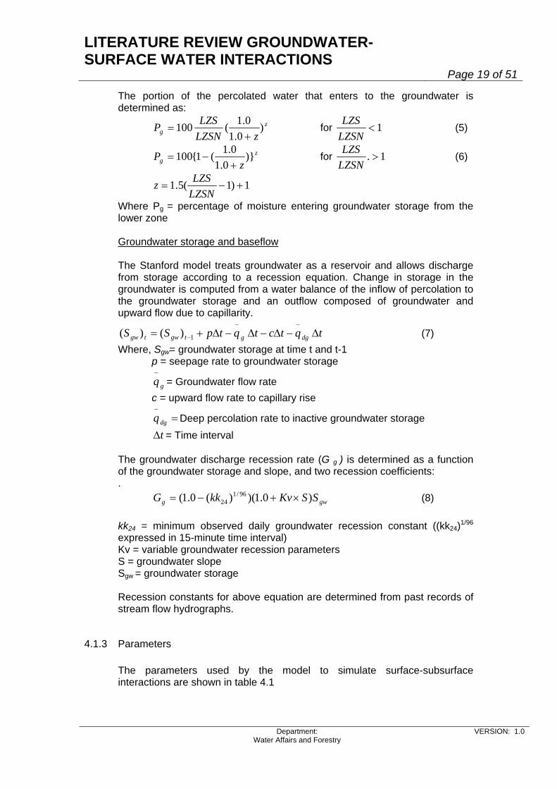
The portion of the percolated water that enters to the groundwater is determined as:
zg zLZSN
LZSP )0.1
0.1(100+
= for 1<LZSNLZS
(5)
zg z
P )}0.1
0.1(1{100+
−= for 1. >LZSNLZS
(6)
1)1(5.1 +−=LZSNLZSz
Where Pg = percentage of moisture entering groundwater storage from the lower zone Groundwater storage and baseflow The Stanford model treats groundwater as a reservoir and allows discharge from storage according to a recession equation. Change in storage in the groundwater is computed from a water balance of the inflow of percolation to the groundwater storage and an outflow composed of groundwater and upward flow due to capillarity.
tqtctqtpSS dggtgwtgw Δ−Δ−Δ−Δ+=−−
−1)()( (7) Where, Sgw= groundwater storage at time t and t-1 p = seepage rate to groundwater storage
= Groundwater flow rate gq−
c = upward flow rate to capillary rise
Deep percolation rate to inactive groundwater storage =−
dgq = Time interval tΔ The groundwater discharge recession rate (G g ) is determined as a function of the groundwater storage and slope, and two recession coefficients: . (8) gwg SSKvkkG )0.1)()(0.1( 96/1
24 ×+−= kk24 = minimum observed daily groundwater recession constant ((kk24)1/96 expressed in 15-minute time interval) Kv = variable groundwater recession parameters S = groundwater slope Sgw = groundwater storage Recession constants for above equation are determined from past records of stream flow hydrographs.
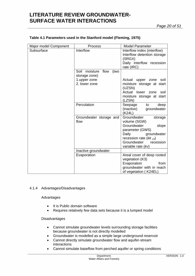
4.1.3 Parameters The parameters used by the model to simulate surface-subsurface interactions are shown in table 4.1
LITERATURE REVIEW GROUNDWATER-SURFACE WATER INTERACTIONS
Page 20 of 51
Department: Water Affairs and Forestry
VERSION: 1.0
Table 4.1 Parameters used in the Stanford model (Fleming, 1975)
Major model Component Process Model Parameter
Interflow Interflow index (interflow) Interflow detention storage (SRGX) Daily interflow recession rate (IRC)
Soil moisture flow (two storage zone) 1.upper zone 2. lower zone
Actual upper zone soil moisture storage at start (UZSN) Actual lower zone soil moisture storage at start (LZSN)
Percolation Seepage to deep (inactive) groundwater (K24L)
Groundwater storage and flow
Groundwater storage volume (SGW) Groundwater slope parameter (GWS) Daily groundwater recession rate (kk 24) Groundwater recession variable rate (kv)
Inactive groundwater
Subsurface
Evaporation Areal cover of deep rooted vegetation (K3) Evaporation from groundwater with in reach of vegetation ( K24EL)
4.1.4 Advantages/Disadvantages Advantages
• It is Public domain software • Requires relatively few data sets because it is a lumped model
Disadvantages
• Cannot simulate groundwater levels surrounding storage facilities because groundwater is not directly modelled
• Groundwater is modelled as a simple large underground reservoir • Cannot directly simulate groundwater flow and aquifer-stream
interactions • Cannot simulate baseflow from perched aquifer or spring conditions
LITERATURE REVIEW GROUNDWATER-SURFACE WATER INTERACTIONS
Page 21 of 51
Department: Water Affairs and Forestry
VERSION: 1.0
• Cannot simulate transmission losses • Cannot account for position of abstraction boreholes on baseflow
depletion • The model is not tested for South African situations
4.2 SWAT (Soil and Water Assessment Tool)
4.2.1 Introduction Type of model: Lumped Input: Daily rainfall, monthly or daily pan evaporation Output: Daily stream flow, daily summary Model Scale: Meso scale to macro scale SWAT was developed to predict the impact of land management practices on water, sediment and agricultural chemical yields in large complex watersheds with varying soils, land use and management conditions over long periods of time. SWAT evolved from the CREAMS and SWRRB models by adding simplified stream flow routing and groundwater components for large basins. It is a quasi-distributed physical model (http://www.brc.tamus.edu/swat/). The basin can be subdivided into sub-basins and each sub-basin is taken as a lumped unit. It is a continuous time scale model using a daily time step. Its components can be grouped into eight major divisions, namely weather (climate), hydrology, sediment, crop growth, soil temperature, nutrient, pesticide and agricultural management. Input information for each sub-basin is grouped or organized into the following categories: weather or climate; unique areas of land cover, soil, and management within the sub-basin (hydrologic response units or HRUs); ponds/reservoirs; groundwater; and the main channel, or reach, draining the sub-basin.
4.2.2 Simulation of processes SWAT consists of canopy storage, infiltration, redistribution, evapotranspiration, lateral subsurface runoff, surface runoff, pond and tributary channel functions. SWAT simulates the redistribution of water in the soil profile using storage routing techniques. Water percolates from one layer to another when the upper layer reaches its field capacity. Upward movement of soilwater is governed by the ratio of soil water and field capacity between two layers. Interflow originates below the surface but above the zone where rocks are saturated with water. Lateral subsurface flow in the soil profile (0-2m) is calculated simultaneously with redistribution. A kinematics storage model is used to predict lateral flow in each soil layer. The model accounts for variation in hydraulic conductivity, slope and soil water content. It also allows for flow upward to an adjacent layer or to the surface.

LITERATURE REVIEW GROUNDWATER-SURFACE WATER INTERACTIONS
Page 22 of 51
Department: Water Affairs and Forestry
VERSION: 1.0
In SWAT, channels are categorized into tributaries and the main channel. Tributary channels are minor or lower order channels branching off the main channel within the sub-basin. Each tributary channel within a sub-basin drains only a portion of the sub-basin and does not receive groundwater baseflow. All flow in the tributary channels is released and routed through the main channel of the sub-basin. SWAT uses the attributes of tributary channels to determine the time of concentration for the sub-basin. SWAT simulates baseflow by categorising the aquifer into a shallow, unconfined aquifer that contributes return flow to streams within the watershed, and a deep, confined aquifer which contributes return flow to streams outside the watershed. Water percolating past the bottom of the root zone is partitioned into two fractions to distribute recharge to the local and regional aquifers. In addition to return flow, water stored in the shallow aquifer may replenish moisture in the soil profile under very dry conditions or be directly removed by plant uptake (only trees may uptake water from the shallow aquifer). Water in the shallow aquifer may also seep into the deep aquifer or be removed by pumping. Water in the deep aquifer may be removed by pumping. A recession constant derived from daily stream flow record is used to lag groundwater flow from the aquifer to stream. SWAT models the groundwater component as a lumped system, and thus is not detailed enough to handle distributed parameters and variable pumping, and hence groundwater levels cannot be simulated accurately. Therefore, by replacing the groundwater component of SWAT with the more detailed and sophisticated groundwater simulator MODFLOW, Sophocleous et-al (1999) and Sophocleous and Perkins (2000) constructed a comprehensive basin model called SWATMOD. The model was developed as a low flow model. SWATMOD uses linking utilities to transfer data between the two models. The model can be run from SWAT or MODFLOW.
4.2.3 Advantages/Disadvantages Advantages
• It simulates most of the hydrological components • Can account for recharge to a regional aquifer that does not discharge
in the sub-catchment • Allows evapotranspiration from a local aquifer • It is public domain software
Disadvantages
• Cannot directly simulate groundwater-streamflow interaction but uses a recession constant to simulate baseflow
• Cannot simulate groundwater levels • Groundwater is modelled as a simple large underground reservoir • Cannot simulate baseflow from perched aquifer or spring conditions • Cannot simulate transmission losses • Cannot account for position of abstraction boreholes on baseflow
depletion

LITERATURE REVIEW GROUNDWATER-SURFACE WATER INTERACTIONS
Page 23 of 51
Department: Water Affairs and Forestry
VERSION: 1.0
• Baseflow is only generated in lower catchment • Not yet tested under South African conditions
4.3 SHE (SHETRAN) Model and MIKE-SHE
4.3.1 Introduction Model type: Physically based, distributed Scale: Micro catchment (made to include all scales in MIKE SHE) SHE (Systeme Hydrologique Europeen) is a physical based distributed model, which was developed in collaboration by three European organizations namely, the Institute of Hydrology, UK, Danish Hydraulic institute, and the French consultant SOGREAH around end of 70’s (Abbot. et-al, 1986a, b). This model was mainly created to simulate the impact of human activities on the hydrologic cycle and hence on water resources development and management. It also incorporates contaminant migration and sediment transport, in which case it is given the name SHETRAN (Parkin et al., 1996). An extended version of the SHE model called MIKESHE was developed to avoid the model limitation in regard to catchment size (DHI, 2001). The latest development to this model was made for the South Florida Water Management District (SFWD) by interlinking MIKESHE and a hydraulic mode MIKE 11 to efficiently simulate surface water-groundwater interactions (DHI, 2001). The model distributes catchment parameters, rainfall input and hydrological response by representing the catchment horizontally and vertically using a Finite Difference grid. Each phase of the hydrological cycle (Interception, Evaporation, snowmelt, overland and channel flow, unsaturated and saturated flow, (figure 4.2) are modelled in time steps based on the finite difference equation of continuity of mass, momentum and energy and empirical formulae established from previous research findings. The principles used in the model and the evolution of each component is described in detail in Abbott et-al (1986a, b). The model structure is shown in Figure 4.2

LITERATURE REVIEW GROUNDWATER-SURFACE WATER INTERACTIONS
Page 24 of 51
Department: Water Affairs and Forestry
VERSION: 1.0
Figure 4.2 SHE model structure ( Abbot, et-al 1986)
4.3.2 Algorithms to simulate interactions Unsaturated Zone In the SHE model, flow in the unsaturated zone is determined by soil moisture content and tension distributions. This zone extends from ground surface to the phreatic zone. Its lower boundary varies through time depending on the amount of water percolating to the phreatic zone. SHE assumes that flow in the unsaturated zone is essentially vertical; hence interflow cannot be accommodated. Based on this assumption flow in this zone is obtained using the one-dimensional Richards’s equation, which is solved by the implicit finite difference scheme. A mass balance equation determines the exchange with the saturated zone. Saturated Zone SHE assumes the flow in the saturated zone is essentially horizontal. The variation in time of the phreatic surface level at each grid is modelled by the non-linear Boussinesq equation, which combines Darcy’s law and the mass conservation of two-dimensional laminar flow in an isotropic heterogeneous aquifer using parameters of specific yield, hydraulic conductivities in x and y directions, saturated thickness and vertical recharge to solve for the phreatic surface level in each grid cell.

LITERATURE REVIEW GROUNDWATER-SURFACE WATER INTERACTIONS
Page 25 of 51
Department: Water Affairs and Forestry
VERSION: 1.0
Abbott et-al (1986 b) indicates the capability of the model to simulate stream water and groundwater interactions under the following conditions:
• phreatic surface in direct contact with a flowing stream • phreatic surface in direct contact with a dry stream • phreatic surface lying below a flowing a stream; • phreatic surface lying below a dry stream
The interaction of stream flow and groundwater is achieved by assigning a hydraulic conductivity to the bed and sides of the channel stream.
4.3.3 Parameters SHE surface-subsurface interaction parameters are shown in table 4.2.
Table 4.2 SHE model parameters Model Component Input Model parameters
Soil moisture tension/ content relationship
Unsaturated Zone
Unsaturated hydraulic conductivity as a function of soil moisture content Porosities or specific yields
Saturated Zone Impermeable bed elevation Specified flows or potential at boundaries Pumping and recharge data
Saturated hydraulic conductivities
Ground surface elevation Impermeable bed elevation Distribution codes for rainfall and metrological source stations
Frame
Distribution code for soil and vegetation
4.3.4 Advantages/Disadvantages Advantages
• Can simulate rapidly changing groundwater levels as it models groundwater piezometric surface
• Can simulate groundwater baseflow and transmission loses • Can provide a water budget for the full hydrologic cycle

LITERATURE REVIEW GROUNDWATER-SURFACE WATER INTERACTIONS
Page 26 of 51
Department: Water Affairs and Forestry
VERSION: 1.0
• Capable of modelling common type hydraulic control structures with appropriate on off triggers (weirs, gates, pumps, etc.)
Disadvantages
• Cannot generate any baseflow for situations where groundwater is below stream channel
• Does not have the ability to handle variable grids • Has not been tested for South African conditions • Very data intensive and requires highly skilled user • Cannot separate baseflow from interflow, perched aquifer or spring
conditions 4.4 MODFLOW
4.4.1 Introduction Type of model: Distributed, physically based Input: aquifer hydraulic parameters, recharge, maximum
evaporation Output: Water levels, groundwater balance Model Scale: Micro to Meso scale MODFLOW is a groundwater model that simulates groundwater flow in confined and unconfined aquifers in three dimensions. It is the most widely used and accepted groundwater model internationally. The model utilises distributed input and variables such as hydraulic conductivity, storativity, recharge and evaporation to simulate groundwater flow using a range of Finite Difference solvers. Being a modular model, additional packages can be easily incorporated to enhance its capability.
4.4.2 Algorithms to simulate interactions Some of the packages used in addressing surface water and groundwater interactions in MODFLOW are (DHI, 2001): Groundwater baseflow and transmission losses These processes can be simulated using the River Package. The River package is used to simulate the flow between an aquifer and surface-water features, such as rivers, lakes or reservoirs. This package contains routines that calculate flow between a river and an underlying aquifer based on the head difference and sediment conductance using the following parameters:
• Hydraulic conductance of the riverbed CRIV [L2/T] • Head in the river HRIV [L], and • Elevation of the bottom of the riverbed RBOT [L].
If the hydraulic head (h) in a cell containing a river is greater than RBOT, the rate of leakage (QRIV) from the river to the aquifer is calculated by:
LITERATURE REVIEW GROUNDWATER-SURFACE WATER INTERACTIONS
Page 27 of 51
Department: Water Affairs and Forestry
VERSION: 1.0
QRIV = CRIV · (HRIV - h) h>RBOT (9) For the case where h is greater than HRIV, QRIV is negative. It means that water flows from the aquifer into the river and is removed from the groundwater model. When h has fallen below the bottom of the riverbed, the rate of leakage through the riverbed is given by: QRIV = CRIV · (HRIV - RBOT) h<= RBOT (10) The value CRIV of a river-cell is often given by: CRIV = (K · L · W) / M (11) Where the value K is the hydraulic conductivity of the riverbed material, L is the length of the river within a cell, W is the width of the river and M is the thickness of the riverbed. If CRIV is unknown, it must be adjusted during a model calibration. This package is not a true surface water flow model, as water in the channel is not directly simulated. The river is treated as an infinite source of water of constant head; hence the package has an inherent problem of being able to generate more transmission losses than there is water in the channel. In addition, the package cannot cater for situations where fluctuations in river stage result in variations in baseflow or flow reversals. To overcome the problem of lack of conservation of mass in the river package, the Stream-Routing Package can be used instead. This package tracks the flow in one or more streams and permits two or more streams to merge into one with flow in the merged stream equal to the sum of the tributary flows. The program also permits diversion from streams. The Streamflow-Routing package (Prudic, 1989) is designed to account for the amount of flow in streams and to simulate the interaction between surface streams and groundwater. Streams are divided into segments and reaches. Each reach corresponds to individual cells in the finite-difference grid. A segment consists of a group of reaches connected in downstream order. Streamflow is accounted for by specifying flow for the first reach in each segment, and then computing streamflow to adjacent downstream reaches in each segment as inflow in the upstream reach plus or minus leakage from or to the aquifer in the upstream reach. The accounting scheme used in this package assumes that streamflow entering the modelled reach is instantly available to downstream reaches. This assumption is generally reasonable because of the relatively slow rates of groundwater flow. If a segment is a diversion, then the specified flow into the first reach of the segment is subtracted from flow in the main stream. However, if the specified flow of the diversion is greater than the flow out of the segment from which flow is to be diverted, then no flow is diverted from that segment. Streamflow and interactions are calculated based on the following parameters:

LITERATURE REVIEW GROUNDWATER-SURFACE WATER INTERACTIONS
Page 28 of 51
Department: Water Affairs and Forestry
VERSION: 1.0
• Streamflow [L3/T] is specified only for the first reach in each segment. • Stream Stage [L] is the head in the stream. • Streambed hydraulic conductance CSTR, which is calculated in the
same way as eq. 11 • Elevation of the Streambed Top • Elevation of the Streambed Bottom • Width of the Stream Channel • Slope of the Stream Channel • Manning's n roughness coefficient
Leakage to or from the aquifer through the streambed is computed in the same way as the river package (eqs. 9 and 10), however HRIV is no longer a parameter but allowed to vary. Stage is calculated from routed flow in the river using Manning’s equation, under the assumption of a rectangular stream channel. The Wetland Package is capable of simulating flow routing, the export/import of water to wetlands, groundwater interflow, and evaporation from wetlands. Surface water flow can be either overland/vegetation plain flow (in forested areas) or channelled/preferential flow. Its use requires a large number of parameters to be quantified; hence it is not applicable at more than a local scale. Groundwater - reservoir or lake interactions The Reservoir Package contains routines to calculate water budgets for water bodies that overly many groundwater cells. The package updates water level, volume and areas as a result of the computed water budget. This package is useful in predicting the effect of certain types of subsurface developments, such as well pumping or mining, on nearby water bodies. For reservoirs that include two or more areas of lower elevation separated by areas of higher elevation, the filling of part of the reservoir may occur before spilling over to an adjacent area. The following parameters are required:
• Land-surface elevation of the reservoir BRES [L], • Vertical hydraulic conductivity of the reservoir bed HCres [L/T], • Thickness of the reservoir bed Rbthick [L] • The elevation of the water table in reservoirs can be specified, by
using a Stage-Time Table. At cells in which reservoir stage exceeds land-surface elevation within the specified reservoir area, the reservoir package is activated. Similarly, wherever reservoir stage is less than the land-surface elevation of a cell, the reservoir package is not activated. If reservoir stage drops below the lowest land-surface elevation for all cells within the specified reservoir area, water exchange is not simulated between the reservoir and the underlying groundwater system. In active cells, water exchange between surface water and groundwater is computed in a manner identical to the River package (eqs. 9 and 10). The

LITERATURE REVIEW GROUNDWATER-SURFACE WATER INTERACTIONS
Page 29 of 51
Department: Water Affairs and Forestry
VERSION: 1.0
Reservoir package is ideally suited for cases where leakage from or to reservoirs may be a significant component of flow in a groundwater system. However, if reservoir stage is unknown, then a more complex conceptualisation would be needed in which reservoir stage would be computed as part of the simulation, rather than having stage be specified as a model input. For reservoirs, where the stage is unknown, Cheng and Anderson (1993), has written a program, which computes the stage in lakes, based on inflows and outflows. Leakage between the reservoir and the underlying groundwater system is simulated for each model cell corresponding to the inundated area by multiplying the head difference between the reservoir and the groundwater system by the hydraulic conductance of the reservoir bed. Hydraulic conductance of the reservoir bed is given by: CRES = HCres · DELC(I) · DELR(J) / Rbthick (12) Where DELC(I) is the width of the model row I, DELR(J) is the width of the model column J. Reservoir bed thickness is subtracted from the land-surface elevation of the reservoir to obtain the elevation of the base of the reservoir-bed sediments. The elevation of the base of the reservoir-bed sediments is used in computing leakage. When the head in the groundwater system is above the base of the reservoir-bed sediments, leakage QRES [L3/T] from or to the groundwater system is computed by: QRES = CRES (HRES - h) (13) Where HRES is the reservoir stage [L] and h is the groundwater head [L]. When the head in the groundwater system is less than the elevation of the base of the reservoir-bed sediments, leakage from the reservoir to the groundwater system is computed by: QRES = CRES (HRES - HRESBOT) (14) Where HRESBOT is the elevation of the base of the reservoir-bed sediments [L]. Springs The Drain Package can be used to simulate springs that discharge water when the regional water table rises above a specified elevation. Discharge is simulated using the following parameters:
• Drain hydraulic conductance (Cd) [L2/T], • Elevation of the Drain (d) [L]
When the hydraulic head h in a drain-cell is greater than the drain elevation, water flows into the drain and is removed from the groundwater model. Discharge to the drain is zero when the hydraulic head is lower than or equal to the median drain elevation. Recharge from the drain is always zero,

LITERATURE REVIEW GROUNDWATER-SURFACE WATER INTERACTIONS
Page 30 of 51
Department: Water Affairs and Forestry
VERSION: 1.0
regardless of the hydraulic head in the aquifer. Discharge rate to the drain (Qd) is calculated by Qd = Cd · (h - d) (15) The value Cd of a drain-cell is often given by Cd = K · L (16) Where L is the length of the drain within a cell. The value K is an equivalent hydraulic conductivity describing all of the head loss between the drain and the aquifer. It depends on the material and characteristics of the drain itself and the immediate environment. The value Cd is usually unknown and must be adjusted during a model calibration. The drain package can be utilised to simulate gravity and artesian springs, but cannot simulate springs that are not in continuity with the regional groundwater body.
4.4.3 Parameters MODFLOW surface-subsurface interaction parameters are listed in table 4.3.
Table 4.3. Table of of MODFLOW parameters
Model Component
Process Model parameters
Hydraulic conductance Head in the river
River Package Groundwater baseflow transmission losses
Elevation of the bottom of the riverbed Upstream inflow Streambed hydraulic conductance Elevation of the Streambed Top
Elevation of the Streambed Bottom Width of the Stream Channel Slope of the Stream Channel
Stream Routing Package Groundwater baseflow Transmission losses
Manning's n roughness coeff Drain hydraulic conductance Drain Package Springs Elevation of the drain Land-surface elevation of the reservoir Vertical hydraulic conductivity of the reservoir bed Thickness of the reservoir bed
Reservoir Seepage from reservoirs
Stage-Time Table

LITERATURE REVIEW GROUNDWATER-SURFACE WATER INTERACTIONS
Page 31 of 51
Department: Water Affairs and Forestry
VERSION: 1.0
4.4.4 Advantages/Disadvantages Advantages
• Can simulate rapidly changing groundwater levels surrounding storage facilities
• Can simulate groundwater baseflow and transmission losses • Capable of easily exchanging data with water quality models
Disadvantages
• Cannot provide a water budget for the full hydrologic cycle because overland flow and the unsaturated zone are not simulated
• Not capable of modelling common type surface water hydraulic control structures with appropriate on-off triggers (weirs, gates, pumps, etc.)
• Requires good data and recharge and aquifer hydraulic parameters if baseflow is to be calibrated
• Cannot simulate baseflow from high lying springs not in hydraulic connection with the aquifer
• Cannot generate a time series of baseflow unless a time series of recharge is available
4.5 Pitman Model – WRSM2000
Type of model: Lumped Input: Monthly rainfall, monthly pan evaporation Output: Monthly flow volumes Model Scale: Meso to macro scale
4.5.1 Introduction The Pitman model is a coarse time scale model that utilises two inputs, monthly precipitation in terms of mean annual percentage and monthly potential evapotranspiration (Pitman, 1973) to simulate monthly runoff. Precipitation is distributed in time using a symmetric S shape cumulative mass curve rainfall. In the SPATSIM version of the model, a rainfall distribution factor parameter (RDF) is incorporated to distribute rainfall into a cumulative mass curve using 4 iterations (Hughes, 1997).
4.5.2 Algorithms to simulate interactions Originally, the model consisted of eleven catchment parameters (table 4.4) to simulate runoff, which are distributed into sub-catchments. Interception is determined as a function of an interception parameter (IP). Surface runoff is generated separately for impervious areas, which are expressed as a proportion of the total sub-catchment. That portion of rainfall directly generates runoff.

LITERATURE REVIEW GROUNDWATER-SURFACE WATER INTERACTIONS
Page 32 of 51
Department: Water Affairs and Forestry
VERSION: 1.0
For the impervious portion, infiltration is calculated as a function of a triangular frequency distribution, which is expressed by parameters ZMIN and ZMAX. In SPATSIM ZAVE is included to stipulate an asymmetry to the distribution. Runoff is generated from two sources, the soil and groundwater. Infiltration increases the level of soil moisture. The runoff Q from soil moisture storage S, or interflow, is determined from a power function (POW) of the ratio of actual soil storage less the parameter of minimum soil moisture storage below which there is no runoff (SL), to the maximum soil moisture storage expressed as a parameter ST (eq. 17). FT represents a parameter of the maximum runoff depth, which occurs at maximum soil storage.
POW
LT
L
SSSSFTQ )(−−
= (17)
Runoff from groundwater is determined by a parameter factor GW, which is the maximum groundwater runoff. This value is subtracted from Q to allocate a portion of runoff to groundwater baseflow. However, there is no firm theoretical background to set this parameter value (Hughes, 1997). The model considers a portion of soil moisture flow to be groundwater discharge and lags it to a higher degree than the remaining component of soil moisture runoff using the Muskingum equation.
4.5.3 Parameters The surface-subsurface interaction parameters of the Pitman model are listed in Table 4.4.
Table 4.4 Pitman model parameters with some additional parameters adopted from Hughes (1997)
Model Component
Process Parameters
Minimum catchment absorption rate Average catchment absorption rate Maximum catchment absorption rate Maximum moisture storage capacity Minimum moisture storage below which there is no runoff Runoff from soil storage at full capacity
Soil Soil moisture runoff
Power of moisture storage-runoff equation
Groundwater Groundwater baseflow
Maximum groundwater runoff
Routing Runoff routing Lag of runoff components (TL for surface and soil runoff, GL for groundwater runoff)
4.5.4 Advantages/Disadvantages Advantages

LITERATURE REVIEW GROUNDWATER-SURFACE WATER INTERACTIONS
Page 33 of 51
Department: Water Affairs and Forestry
VERSION: 1.0
• Widely applicable and well tested for South African conditions • require few and well documented data input • simulates long time series
Disadvantages
• Cannot simulate unsaturated flow, groundwater storage and groundwater flow
• It has no facility to exchange data with water quality models • Cannot directly simulate groundwater-streamflow interaction but uses
a parameter to distribute a portion of soil moisture baseflow to groundwater
• Cannot simulate groundwater levels • Cannot simulate baseflow from perched aquifer or spring conditions • Cannot simulate transmission losses • Cannot account for position of abstraction boreholes on baseflow
depletion
4.6 ACRU Model Type of model: Lumped Input: Daily rainfall, daily pan evaporation or meteorological
data Output: Daily runoff Model Scale: Micro to macro scale
4.6.1 Introduction ACRU (agricultural catchment research unit) (Figure 4.3) is an agro- hydrological model (Schulze, 1995) that simulates daily runoff. It is a lumped model ideal for sub-catchment sizes not exceeding 30 square kilometres. The limitation of the sub-catchment size is due to the SCS (US Soil Conservation Service) method that is used to simulate runoff.
4.6.2 Algorithms to simulate interactions The heart of the ACRU model is a daily multi-layer soil water budget (Schulze, 1995). Infiltration into the soil drains to a lower soil layer when the upper layer exceeds a field capacity parameter. Upward soil water movement due to capillary rise occurs depending on the relative wetness of adjacent soil horizons in the root zone. The following parameters are required to simulate the soil water budget:
• Total soil porosity • Field capacity • Permanent wilting point • Thickness of top soil horizon

LITERATURE REVIEW GROUNDWATER-SURFACE WATER INTERACTIONS
Page 34 of 51
Department: Water Affairs and Forestry
VERSION: 1.0
Inputs Location Catchment Climate Hydrological Land Change Agronomic Reservoir Land use Soil Irrigation Supply Irrigation demand
Model ACRU MODEL Operational
Models
Point or Lumped or Distributed Models or GIS linked
Dynamic Time Or
Annual Cyclic Change
Soil Water Budgeting/ Total Evaporation Modelling
Simulation Options/ Combinations
Runoff Reservoir Status
Sediment Yield
Irrigation Demand Irrigation Supply Land Use Impacts
Climate Change
Crop Yield
Daily • • • • • • • • Monthly • • • • • • • • Annually • • • • • • • •
Output
Risk Analysis
• • • • • • •
Specific Objective/ Components
Stormflow Baseflow Peak discharge Hydrograph -generation -routing EV analyses
Outflows: -Overflow -normal flow -seepage -abstraction Interbasin transfers Off-channel storage
Sediment -Generation Reservoir -Siltation
Crop demand Application: -On demand -fixed cycle -fixed amount -deficit
From: -Reservoir -river -river and reservoir -off channel storage -return flow
Gradual change Abrupt change Total Evaporation Tillage Practices Wetlands
ΔCO2 ΔT ΔE ΔP
Maize Winter Wheat Sugarcane Primary Productivity -dry land -irrigated -profit/loss
Figure 4.3 The ACRU agro hydrological modelling system: concepts
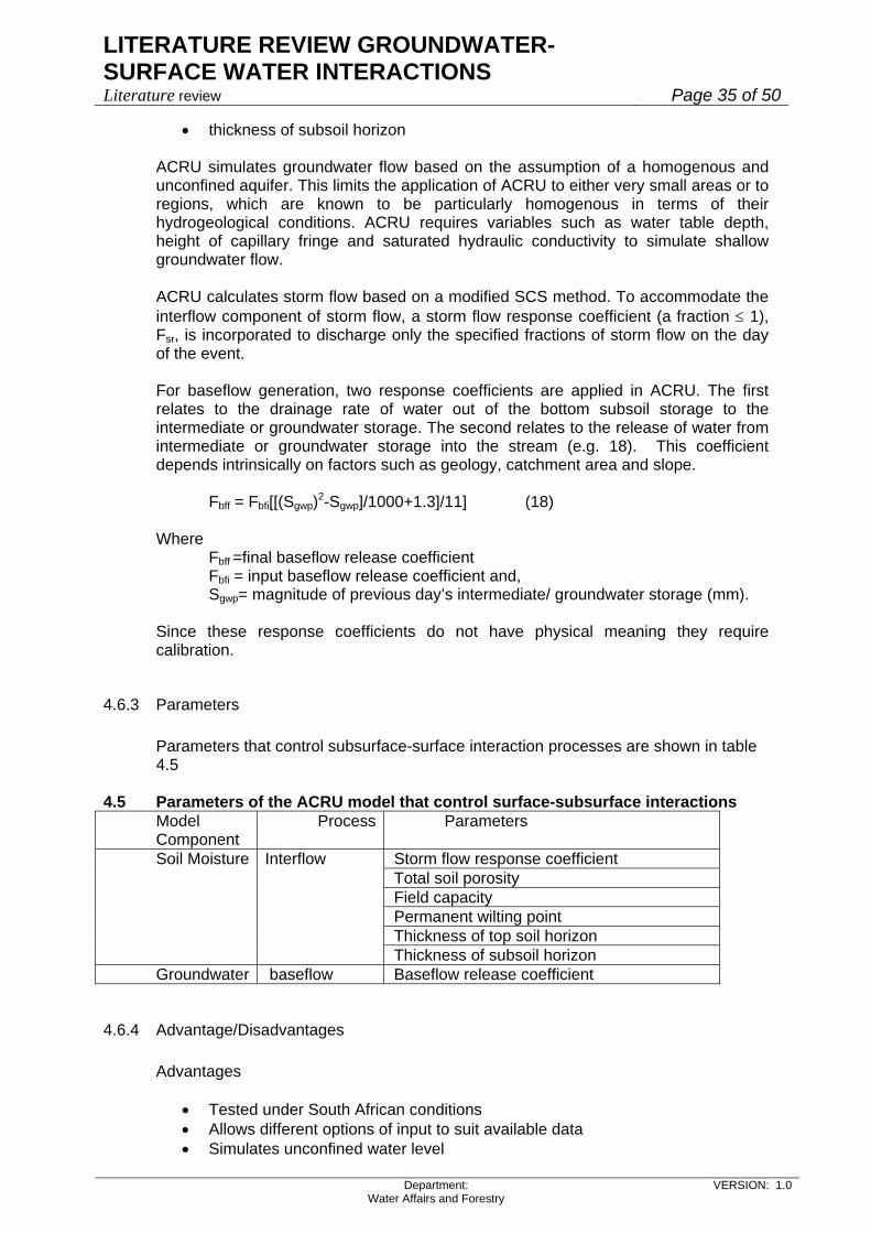
LITERATURE REVIEW GROUNDWATER-SURFACE WATER INTERACTIONS
Literature review Page 35 of 50
Department: Water Affairs and Forestry
VERSION: 1.0
• thickness of subsoil horizon ACRU simulates groundwater flow based on the assumption of a homogenous and unconfined aquifer. This limits the application of ACRU to either very small areas or to regions, which are known to be particularly homogenous in terms of their hydrogeological conditions. ACRU requires variables such as water table depth, height of capillary fringe and saturated hydraulic conductivity to simulate shallow groundwater flow. ACRU calculates storm flow based on a modified SCS method. To accommodate the interflow component of storm flow, a storm flow response coefficient (a fraction ≤ 1), Fsr, is incorporated to discharge only the specified fractions of storm flow on the day of the event. For baseflow generation, two response coefficients are applied in ACRU. The first relates to the drainage rate of water out of the bottom subsoil storage to the intermediate or groundwater storage. The second relates to the release of water from intermediate or groundwater storage into the stream (e.g. 18). This coefficient depends intrinsically on factors such as geology, catchment area and slope. Fbff = Fbfi[[(Sgwp)2-Sgwp]/1000+1.3]/11] (18) Where Fbff =final baseflow release coefficient Fbfi = input baseflow release coefficient and, Sgwp= magnitude of previous day’s intermediate/ groundwater storage (mm). Since these response coefficients do not have physical meaning they require calibration.
4.6.3 Parameters Parameters that control subsurface-surface interaction processes are shown in table 4.5
4.5 Parameters of the ACRU model that control surface-subsurface interactions Model Component
Process Parameters
Storm flow response coefficient Total soil porosity Field capacity Permanent wilting point Thickness of top soil horizon
Soil Moisture Interflow
Thickness of subsoil horizon Groundwater baseflow Baseflow release coefficient
4.6.4 Advantage/Disadvantages Advantages
• Tested under South African conditions • Allows different options of input to suit available data • Simulates unconfined water level

LITERATURE REVIEW GROUNDWATER-SURFACE WATER INTERACTIONS
Literature review Page 36 of 50
Department: Water Affairs and Forestry
VERSION: 1.0
Disadvantages • Cannot simulate aquifer-stream interactions since baseflow is simulated only
by recession constants • Cannot simulate confined groundwater flow and storage • Cannot simulate baseflow from perched systems or spring conditions • Cannot simulate rapidly changing groundwater levels surrounding storage
facilities • Cannot simulate transmission losses • Cannot account for position of abstraction boreholes on baseflow depletion
4.7 VTI (Variable Time Interval Simulation Model) Type of model: Semi-distributed Input: 5 minute to daily rainfall, daily or mean monthly pan
evaporation Output: daily runoff Model Scale: Micro to macro scale
4.7.1 Introduction The VTI model is a semi-distributed rainfall-runoff model that takes rainfall input at time steps from 5 minutes up to 1 day. However, due to the scarcity of fine time scale rainfall data, daily rainfall is most commonly used. This is disaggregated to generate hourly rainfall intensities. The VTI model incorporates the following hydrological processes:
• Actual evapotranspiration • Interception • Rainfall intensity controlled runoff • Soil moisture runoff (interflow) • Perched baseflow • Groundwater baseflow • Catchment routing and small dam components • Channel transmission losses • Channel flow routing
The surface-subsurface interaction of the model is briefly explained below based on Sami et-al, (1995) and Hughes (1997).
4.7.2 Algorithms to simulate interactions In the VTI model the soil profile is divided into two layers. In each layer the soil moisture distribution for every sub-catchment at every time interval is represented by a normal distribution. The portion of the area that potentially contributes to groundwater recharge is assumed equivalent to the proportion of the lower soil layer distribution in excess of field capacity. To account for the spatial position of such areas, lateral and vertical distribution factors (LDF and VDF) are calculated for each time step. The proportion of the soil at greater than saturation and field capacity is modified by these distribution factors to estimate a soil saturated seepage face and recharge area. VTI has functions that allow the simulation of the following surface-subsurface interactions:

LITERATURE REVIEW GROUNDWATER-SURFACE WATER INTERACTIONS
Literature review Page 37 of 50
Department: Water Affairs and Forestry
VERSION: 1.0
• Drainage from the portion of the lower zone above field capacity into a percolating storage (recharge) which conceptually represents water in transit to the water table
• Interflow from portions of the upper and lower soil profile at saturation based on a normal soil moisture distribution
• The re-emergence of percolating water as spring water above the regional water table due to structural controls or geological impedance, even when the groundwater level is below surface
• Groundwater baseflow based on piezometric surface dynamics resulting from change in aquifer storage due to increments from percolating storage, lateral transfers to other sub-catchments or out of the modelled domain and borehole abstraction
• Transmission losses into permeable channel bed materials. Recharge Recharge is calculated as; R = LFC X 1/2 X KG X dt (19) Where LFC is the proportion of the lower soil layer above field capacity, with corrections for LDF and VDF. LDF and VDF are used to account for the spatial distribution of source area and vertical distribution of drainage areas in the soil profile, respectively. They range from 0-1. KG is the saturated hydraulic conductivity. Half of the hydraulic conductivity is used to represent vertical drainage under partially saturated conditions. The saturated hydraulic conductivity is computed as: KG (mm hr-1) = TM / Depth x S x 1000 / 24 (20) Where Depth is aquifer thickness (m), TM is transmissivity; S is Storativity (used to adjust saturated hydraulic conductivity (KG) in consideration of the possibility that some of the potential recharge area may not be hydraulically connected to the groundwater body). Perched aquifers and springflow Recharge from the lower soil layer increments is represented by PSTORE, which is a storage zone of water in transit from the soil to groundwater, conceptually representing percolating water. Water in PSTORE, is assumed to be uniformly distributed through the sub-catchment area. Drainage from PSTORE can be either vertically, to the regional groundwater or laterally, as discharge to spring flow directly into the stream channel. A parameter termed the groundwater drainage factor (DVECT) represents the lateral and vertical components of percolation. The proportion of storage that lies above the groundwater drainage vector line (PROP) is calculated geometrically from DVECT, the hydraulic gradient, and the mean catchment slope. PROP represents the fraction of groundwater storage that may re-emerge as springs (PROP). The rate of re-emergence of spring flow is determined as: Re-emergence (mm) = PROP x PSTORE / TOTAL x KG X dt (21) Where TOTAL is the maximum storage of PSTORE defined as the product of PSTORE geometry during that time step and the storativity. This algorithm allows the depletion of springflow as the percolating storage dries.
LITERATURE REVIEW GROUNDWATER-SURFACE WATER INTERACTIONS
Literature review Page 38 of 50
Department: Water Affairs and Forestry
VERSION: 1.0
Recharge to regional aquifer Increments to the regional aquifer increment the hydraulic gradient and are calculated from the fraction of PSTORE that lies below DVECT (PGWATER): Recharge (mm) = PGWATER x PSTORE / TOTAL x KG / ANTY X dt (22) Groundwater baseflow Percolation from PSTORE to the regional groundwater, increments the water table, which is represented by a vector with a slope equal to the hydraulic gradient. If this vector intercepts the ground surface a saturated seepage face is created longitudinally along the channel. Groundwater baseflow is calculated as the product of this seepage face calc, KG and the hydraulic gradient. Subsurface redistribution To allow groundwater transfer between sub-areas, losses from PSTORE to adjacent sub-area are determined as: Transfer (mm) = PTRANS x KG dt / ANTY (23) Where ANTY is an anisotropy factor expressed as ANTY = 900/ Tan-1 (DVECT) (24) Groundwater transfer between sub-areas is determined as: Outflow = Tadj x HGRAD X WIDTH X dt (25) Where: Tadj is the adjusted transmissivity, incremented to account for increasing flow rates as the groundwater depth rises above the rest water level (RWL). HGRD is the hydraulic gradient, which is also incremented as the water table rises, from being close to zero at the RWL and rising exponentially to a maximum defined by the regional groundwater gradient parameter when the piezometric surface intersects the surface.
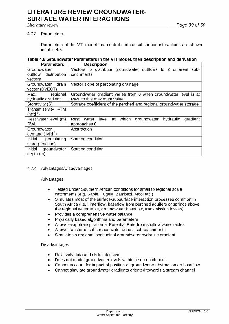
LITERATURE REVIEW GROUNDWATER-SURFACE WATER INTERACTIONS
Literature review Page 39 of 50
Department: Water Affairs and Forestry
VERSION: 1.0
4.7.3 Parameters Parameters of the VTI model that control surface-subsurface interactions are shown in table 4.5
Table 4.6 Groundwater Parameters in the VTI model, their description and derivation Parameters Description
Groundwater outflow distribution vectors
Vectors to distribute groundwater outflows to 2 different sub-catchments
Groundwater drain vector (DVECT)
Vector slope of percolating drainage
Max. regional hydraulic gradient
Groundwater gradient varies from 0 when groundwater level is at RWL to this maximum value
Storativity (S) Storage coefficient of the perched and regional groundwater storage Transmissivity –TM (m2d-1)
Rest water level (m) RWL
Rest water level at which groundwater hydraulic gradient approaches 0.
Groundwater demand ( Mld-1)
Abstraction
Initial percolating store ( fraction)
Starting condition
Initial groundwater depth (m)
Starting condition
4.7.4 Advantages/Disadvantages Advantages
• Tested under Southern African conditions for small to regional scale catchments (e.g. Sabie, Tugela, Zambezi, Mooi etc.)
• Simulates most of the surface-subsurface interaction processes common in South Africa (i.e. : interflow, baseflow from perched aquifers or springs above the regional water table, groundwater baseflow, transmission losses)
• Provides a comprehensive water balance • Physically based algorithms and parameters • Allows evapotranspiration at Potential Rate from shallow water tables • Allows transfer of subsurface water across sub-catchments • Simulates a regional longitudinal groundwater hydraulic gradient
Disadvantages
• Relatively data and skills intensive • Does not model groundwater levels within a sub-catchment • Cannot account for impact of position of groundwater abstraction on baseflow • Cannot simulate groundwater gradients oriented towards a stream channel

LITERATURE REVIEW GROUNDWATER-SURFACE WATER INTERACTIONS
Literature review Page 40 of 50
Department: Water Affairs and Forestry
VERSION: 1.0
4.8 Hydrograph Separation Techniques
4.8.1 Introduction Hydrological separation techniques are used to separate baseflow from total streamflow hydrographs, but generally cannot distinguish between groundwater baseflow and baseflow originating from other subsurface pathways that may not be in hydraulic connection with the regional aquifer. Two types of hydrological techniques are commonly used; chemical and graphical separations.
4.8.2 Chemical methods Conservative constituents such as chloride, hydrogen and oxygen isotopes, or silica that have clearly distinguishable concentrations in surface and subsurface waters are used for hydrograph separations. Once their chemical concentrations in rainfall (assumed to be equivalent to direct runoff), streamflow and groundwater are characterised baseflow is generated as follows: Qg= QT ((Cr-Cd) / (Cg-Cd) (26) Where Qg is base flow volume, QT is the total streamflow; Cd, Cg and Cr are concentrations in surface runoff, groundwater and river, respectively.
4.8.3 Herold method This method was developed by Herold (1980) and is based on the following equation:
PGQDecayQQ igigi ⋅+⋅= −− 11 (27) Where Qg is assumed to be the groundwater contribution. Qi-1 is the total streamflow where the subscripts i and i-1 refer to the current and preceding month. Decay is a groundwater factor (0<Decay<1), and PG a groundwater growth factor (%). Groundwater baseflow Qgi represents the combined effect of previous groundwater after decay (Qgi-1*Decay) and rainfall induced recharge (Qi-1*PG). Having been tested by Pitman and Vegter using flows measured at the Department of Water Affairs and Forestry's gauge No X3H00l on the Sabie River, the method was consequently adopted in the Water Resources 1990 project, in which a time series of monthly flows were separated into surface and groundwater components for each of the approximately 2000 Quaternary catchments of the study area (South Africa, Lesotho and Swaziland) in order to derive a map of groundwater recharge.
4.8.4 Digital Filters Based on Nathan and McMahon (1990), this method uses a filter parameter to separate quick flow (inter flow and storm runoff) from baseflow. The difference between quick flow and total streamflow is assumed to be baseflow. Quickflow is calculated by: qt = aqt-1 + 0.5(1+a)(Qt-Qt-1) (28)

LITERATURE REVIEW GROUNDWATER-SURFACE WATER INTERACTIONS
Literature review Page 41 of 50
Department: Water Affairs and Forestry
VERSION: 1.0
Qbt = Qt-qt
Where q is quick flow, Q is streamflow, Qb is base flow and a is the filter parameter. The filter parameter ranges between 0-1. Smakhtin and Watkins (1997) indicated that acceptable results can be obtained by using a filter parameter of 0.995.
4.8.5 Rational method The rational method was proposed by Smakhtin and Watkins (1997) to overcome the limitation of a digital filter, which was found to have a tendency of overestimating baseflow, especially in highly intermittent streams and for short duration flood events. The method uses nodal points identified from a recession analysis. These nodal points indicate the end of known recession periods where the quickflow is assumed to be zero. By connecting these nodal points a baseflow hydrograph is generated.
4.9 Hydrogeomorphic Approach
4.9.1 Introduction One of the factors that affect streamflow and groundwater interaction is geomorphology. Xu et al. (2003) suggested that it is important to characterise a stream in terms of its geomorphologic features and recommended a geomorphologic classification of streams based on their location in upper, middle and lower areas of a catchment and the type of groundwater and surface water relationships that could take place.
4.9.2 Interactions Based on the above classification Xu et-al (2003) identified six types of geomorphologic streams. They further indicated the significance of each type of stream to the environmental reserve (Figure 4.4 and table 4.7).

LITERATURE REVIEW GROUNDWATER-SURFACE WATER INTERACTIONS
Literature review Page 42 of 50
Department: Water Affairs and Forestry
VERSION: 1.0
Hydrogeomorphologic Approach
• Geomorphologic typing
• Interaction scenarios
• Hydraulic connection
• Baseflowseparation concept
Interflow dominant in upper catchment
Intermittent in middle course
Groundwater discharge zone
Under some circumstances
Q
t
QQQ
ttt
Type 1: upper catchment
Type 2: middle course
Type 3: lower catchment
Type 4: Special cases
Figure 4.4 Hydrogeolmorphological classification of rivers

LITERATURE REVIEW GROUNDWATER-SURFACE WATER INTERACTIONS
Literature review Page 43 of 50
Department: Water Affairs and Forestry
VERSION: 1.0
Table 4.7 Type of interaction between groundwater and rivers ( Xu et-al, 2003) Geomorphologic type Description of Interaction Significance to
Environmental Reserve
A–stream without bank storage
1 interflow dominant No
B-stream controlled by bed morphology
2 Intermittent stream Yes
C–stream with bank storage
3 Effluent streams, bank storage of high river flows( gaining stream )
Yes
D–stream influenced by channel morphology
3 Effluent streams ( gaining stream )
Yes
E–stream controlled by geological structures
3 Effluent streams ( gaining stream )
Yes
F-stream with headwater originating as allogenic source
4 Ephemeral, transmission losses possible
No
Although Xu et-al (2003) emphasise the importance of geomorphologic stream classification in providing information on interaction of groundwater and surface water, the hydraulic connections depicted and the type of interactions are unsuitable to apply under South African conditions for the following reasons:
• Aquifer stream interactions are mainly conceptualised as being oriented perpendicular to the channel rather than longitudinal, as is often the case at regional scale.
• Baseflow is conceptualised as being generated in the lower catchment, whereas in most parts of South Africa baseflow is generated primarily in the wetter upper and steeper reaches of the catchment (e.g. Sabie, Tugela, Orange, etc.). In the lower reaches the groundwater level is commonly below the stream channel and the piezometric surface is oriented longitudinally to the channel, especially when the topographic setting is relatively flat. This misconception has major implications for Reserve determinations since the region of interest is misplaced. This situation is prevalent where higher rainfall occurs in steep headwater regions. In coastal regions receiving high rainfall groundwater drains towards river channels, hence the lower reaches of the channel would contribute to baseflow. It is important to distinguish between these two cases; an aspect which the classification system cannot accommodate.
• Perched or spring dominated baseflow cannot be accommodated
4.9.3 Quantification of Interactions Xu et al. (2003) focus their attention on the lower catchment and assume recharge results in a groundwater gradient oriented towards the stream (Figure 4.5).
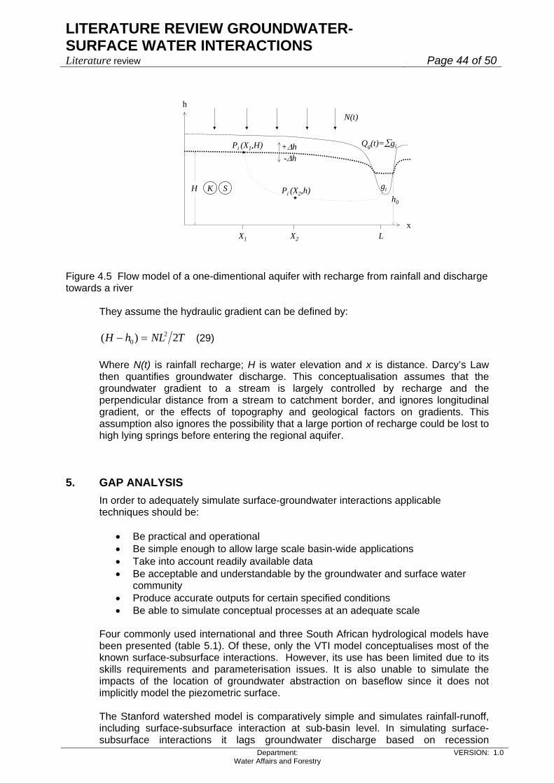
LITERATURE REVIEW GROUNDWATER-SURFACE WATER INTERACTIONS
Literature review Page 44 of 50
Department: Water Affairs and Forestry
VERSION: 1.0
h
xL
+Δh-Δh
N(t)
H K S
Qg(t)=∑giPi (X1,H)
Pi (X2,h) gi
X2
h0
X1
Figure 4.5 Flow model of a one-dimentional aquifer with recharge from rainfall and discharge towards a river
They assume the hydraulic gradient can be defined by:
TNLhH 2)( 20 =− (29)
Where N(t) is rainfall recharge; H is water elevation and x is distance. Darcy’s Law then quantifies groundwater discharge. This conceptualisation assumes that the groundwater gradient to a stream is largely controlled by recharge and the perpendicular distance from a stream to catchment border, and ignores longitudinal gradient, or the effects of topography and geological factors on gradients. This assumption also ignores the possibility that a large portion of recharge could be lost to high lying springs before entering the regional aquifer.
5. GAP ANALYSIS In order to adequately simulate surface-groundwater interactions applicable techniques should be:
• Be practical and operational • Be simple enough to allow large scale basin-wide applications • Take into account readily available data • Be acceptable and understandable by the groundwater and surface water
community • Produce accurate outputs for certain specified conditions • Be able to simulate conceptual processes at an adequate scale
Four commonly used international and three South African hydrological models have been presented (table 5.1). Of these, only the VTI model conceptualises most of the known surface-subsurface interactions. However, its use has been limited due to its skills requirements and parameterisation issues. It is also unable to simulate the impacts of the location of groundwater abstraction on baseflow since it does not implicitly model the piezometric surface. The Stanford watershed model is comparatively simple and simulates rainfall-runoff, including surface-subsurface interaction at sub-basin level. In simulating surface-subsurface interactions it lags groundwater discharge based on recession

LITERATURE REVIEW GROUNDWATER-SURFACE WATER INTERACTIONS
Literature review Page 45 of 50
Department: Water Affairs and Forestry
VERSION: 1.0
coefficients. This limits its applicability in areas where there is no recession coefficient data. Furthermore the lumped nature of the model hampers the effective simulation of discharge or recharge from or through spatially distributed boreholes. However, the concept of re-distributing water through two layers of soil profile is important in conceptualising any alternative model. Similar to the Stanford watershed model SWAT uses recession constants measured from daily stream flow record to lag groundwater discharge. It is superior in that it classifies the aquifer into shallow (unconfined) and deep or confined. The point of discharge for confined aquifers could be out of the catchment area. In addition it classifies channels into a main channel and tributary channels. Tributary channels are lower order channels and hence do not receive groundwater baseflow. It allows interflow through 0 to 2m depth of soil. Another important concept in the SWAT model is that of the hydrological response unit. Hydrological response units are portions of the sub-catchment or catchment that have the same catchment parameters within its boundary. This could be similar topography, land use, soil type, vegetation, and geology. This principle is also applied in the ACRU model. The accuracy of physically distributed models, such as SHE, in simulating hydrological flow in comparison to lumped or quasi-distributed models cannot be argued. However, in most cases their large data requirement outweighs their advantage in regard to reliability and negates their advantages. In addition, because of their data appetite, models such as SHE are mainly applicable at the micro-scale. This problem, however, is resolved in the MIKE SHE model. MIKE SHE is applicable for any catchment where there is a reasonable data set irrespective of catchment size. In the South African context the Pitman model must be acknowledged as the state-of-the-art due to its widespread use and acceptance, ease of parameterisation and acknowledged reliability. However, like most conceptual surface water models, it fails to simulate surface-subsurface interaction accurately and was designed as a surface water resource model. Groundwater models are not suitable to model interactions at anything larger than channel reach scale since they do not model surface runoff and are overly reliant on highly heterogeneous parameters of recharge and conductivity that are difficult to quantify. In addition, simulated head in abstraction and river cells is strongly affected by cell size. Cell sizes must therefore be as small as possible, which is problematic when modelling large areas. Hydrograph separations cannot distinguish between groundwater baseflow, and other types of baseflow and hence will never be able to simulate impacts of groundwater abstraction on baseflow. For this reason, their use to determine the impacts of abstraction on the groundwater component of the Reserve is dubious. Currently, none of the identified methods hold promise for simulating interactions at a regional scale. However, the Pitman Model, if developed to incorporate surface-subsurface interactions and the impacts of groundwater abstraction, holds the most promise of achieving widespread acceptance and desired results. Such algorithms, utilising few parameters, are achievable, as evident from the mechanisms simulated in the VTI model.
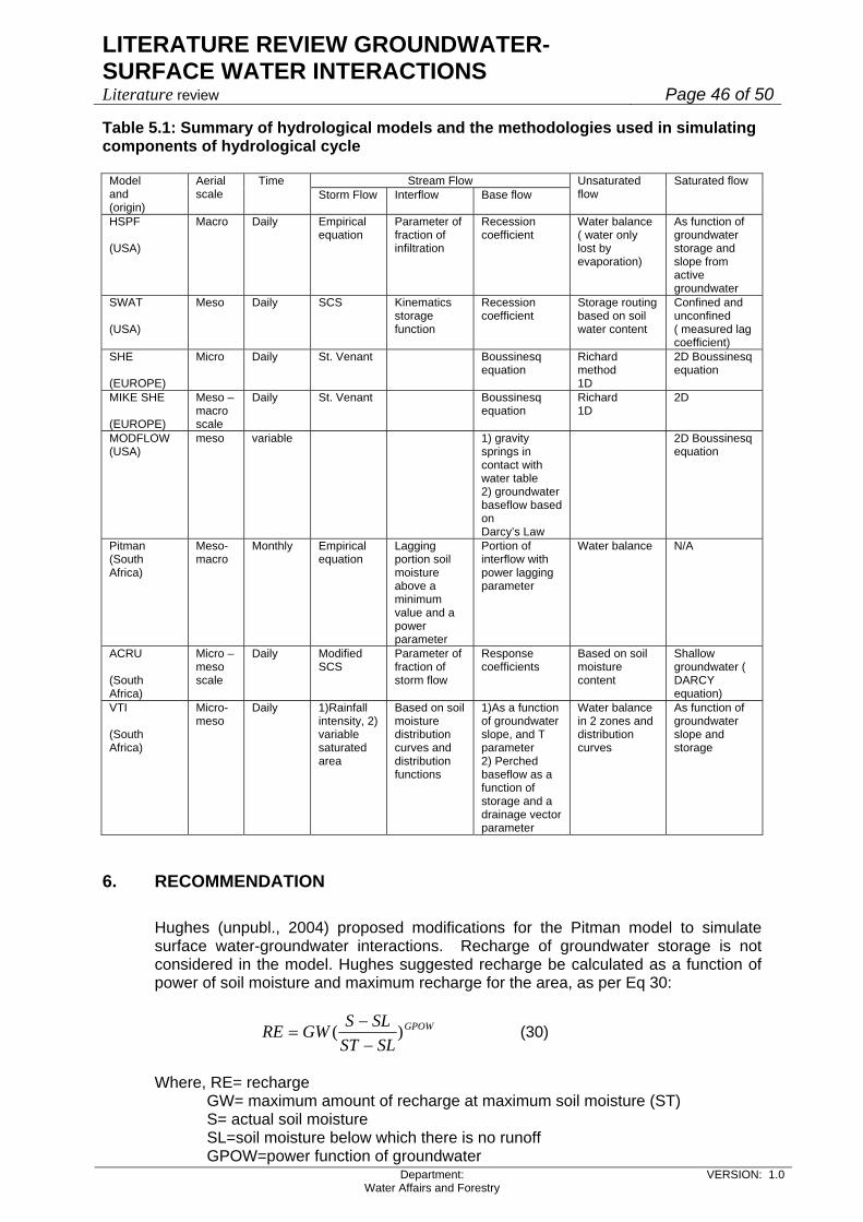
LITERATURE REVIEW GROUNDWATER-SURFACE WATER INTERACTIONS
Literature review Page 46 of 50
Department: Water Affairs and Forestry
VERSION: 1.0
Table 5.1: Summary of hydrological models and the methodologies used in simulating components of hydrological cycle
Stream Flow Model
and (origin)
Aerial scale
Time Storm Flow Interflow Base flow
Unsaturated flow
Saturated flow
HSPF (USA)
Macro Daily Empirical equation
Parameter of fraction of infiltration
Recession coefficient
Water balance ( water only lost by evaporation)
As function of groundwater storage and slope from active groundwater
SWAT (USA)
Meso Daily SCS Kinematics storage function
Recession coefficient
Storage routing based on soil water content
Confined and unconfined ( measured lag coefficient)
SHE (EUROPE)
Micro Daily St. Venant Boussinesq equation
Richard method 1D
2D Boussinesq equation
MIKE SHE (EUROPE)
Meso –macro scale
Daily St. Venant Boussinesq equation
Richard 1D
2D
MODFLOW (USA)
meso variable 1) gravity springs in contact with water table 2) groundwater baseflow based on Darcy’s Law
2D Boussinesq equation
Pitman (South Africa)
Meso-macro
Monthly Empirical equation
Lagging portion soil moisture above a minimum value and a power parameter
Portion of interflow with power lagging parameter
Water balance N/A
ACRU (South Africa)
Micro –meso scale
Daily Modified SCS
Parameter of fraction of storm flow
Response coefficients
Based on soil moisture content
Shallow groundwater ( DARCY equation)
VTI (South Africa)
Micro-meso
Daily 1)Rainfall intensity, 2) variable saturated area
Based on soil moisture distribution curves and distribution functions
1)As a function of groundwater slope, and T parameter 2) Perched baseflow as a function of storage and a drainage vector parameter
Water balance in 2 zones and distribution curves
As function of groundwater slope and storage
6. RECOMMENDATION Hughes (unpubl., 2004) proposed modifications for the Pitman model to simulate surface water-groundwater interactions. Recharge of groundwater storage is not considered in the model. Hughes suggested recharge be calculated as a function of power of soil moisture and maximum recharge for the area, as per Eq 30:
GPOW
SLSTSLSGWRE )(−−
= (30)
Where, RE= recharge GW= maximum amount of recharge at maximum soil moisture (ST) S= actual soil moisture SL=soil moisture below which there is no runoff GPOW=power function of groundwater

LITERATURE REVIEW GROUNDWATER-SURFACE WATER INTERACTIONS
Literature review Page 47 of 50
Department: Water Affairs and Forestry
VERSION: 1.0
The Pitman model also fails to address the discharge of groundwater as springs above the regional groundwater level, to simulate the level of the water table and its relationship to baseflow, groundwater abstraction, and subsurface transfers across catchment boundaries. By adding a few parameters to incorporate some of these concepts in the VTI model, many of these shortcomings could be addressed. In addition, a new sub-routine is required to incorporate the position of major abstraction relative to the stream channel and its effect in surface – groundwater interactions. For this case the theoretical background discussed by Sophocleous (2002) can be incorporated based on simple diffusion curves related to distance, abstraction rate, transmissivity, storativity and duration of pumping. This concept would incorporate the effects of abstraction on interactions and would relate interactions to aquifer diffusivity (T/S) and distance of point of abstraction from the stream. However, further analysis is required to develop an algorithm that incorporates the distribution of boreholes in a catchment. Such a development would be of great relevance to the allocation of abstraction permits when considering potential impacts on the Reserve.

LITERATURE REVIEW GROUNDWATER-SURFACE WATER INTERACTIONS
GLOSSARY Page 48 of 51
Department: Water Affairs and Forestry
VERSION: 1.0
GLOSSARY TERM DEFINITION
LITERATURE REVIEW GROUNDWATER-SURFACE WATER INTERACTIONS
APPENDIX Page 49 of 51
Department: Water Affairs and Forestry
VERSION: 1.0
APPENDIX A: REFERENCE LIST Abbot, M.B, Bathurst, J.C., Cunge, J.A., O’Connell, P.E and Rasmussen, 1986. An introduction to the European Hydrological system –Systeme Hydrologiquae Europeen, “SHE”, 2: structure of a physical –based, distributed modeling system. Abbot, M.B, Bathurst, J.C., Cunge, J.A., O’Connell, P.E and Rasmussen, 1986. An introduction to the European hydrological system –Systeme Hydrologique Europeen, “SHE”, 1: history and philosophy of a physically-based, distributed modeling system. ACT 108, 1997. Republic of South Africa Water Services Act. DHI, 2001. External review results and comparisons of MIKE SHE from the US, DHI Water and Environment, Horsholm, Denmark. http://www.dhisoftware.com/mikeshe/Reviews/index.htm Eckhardt, K. and Arnold, J.G., 2001. Automatic calibration of a distributed catchment model. J.Hydrol. 251: 103-109. Fleming, George 1975. Computer Simulation Techniques in Hydrology. Elsevier. New York. Haevey J.W and Bencala KE., 1993. The effect of stream bed topography on surface-subsurface water exchange in mountain catchments. Water Resources. Res. 29:89-98. Hattermann, F. Krysanova, V. Wechsung, F. and Wattenbach, M., 2004. Integrated groundwater dynamics in regional hydrological modeling. Environmental modeling & software, ELSEVIER. Henrisken, Hans Jorgen, Trodboory, Lras; Nyegpard, Per; Sonnenborg, Torbel Obel; Refsgaorad, Jens Christian; Madsen, Bjaren, 2003. Methodology for construction, calibration and validation of national hydrological model for Denmark. J. Hydro. 280: 52-71 Hughes, DA 1997. Southern Africa “Friend”- The application of rainfall runoff models in SADC Regions. WRC Report No 235/1/97, South Africa. Hughes, DA 2002. Incorporating groundwater recharge and discharge functions into an existing monthly rainfall-runoff model. Institute for water Research, Rhodes University, Grahamstown. Lukey, B.T., Sheffield, J. Bathurst, J.C., Hiley, R.A and Mathys, N., 2000. Test of the SHETRAN technology for modeling the impact of restoration on badlands runoff and sediments yield at Draix, France. J.Hydrol. 235: 44-62. Nield, Simon P., Townley, Lloyd R., and Barr, D., 1994. A framework for quantitative analysis of surface water-groundwater interaction: Flow geometry in a vertical section. Water Res. Res. 30: 2461-2475, South Africa. Parkin, G., O’Donnel, G., Ewen, J., J.C. Bathurst, O’Connell, P.E., and Lavabre, J., 1996. Validation of catchment models for predicting land use and climate change impacts. 2 case study for a Mediterranean catchment. J. Hydrol. 175: 595-613. Rajukar, M.P, Kothari, U.C., and Chaube U.C 2004. Modeling of the daily rainfall-runoff relationship with artificial neural network. J. Hydrol. 285: 96-113.

LITERATURE REVIEW GROUNDWATER-SURFACE WATER INTERACTIONS
APPENDIX Page 50 of 51
Department: Water Affairs and Forestry
VERSION: 1.0
Sami, K and Hughes, D.A., 1996. A comparison of recharge estimates to fractured sedimentary aquifer in South Africa from a chloride mass balance and an integrated surface-subsurface model. J. Hydrol. 179: 111-136. Schulze, RE, 1995. Hydrology and agro hydrology: A text to accompany the ACRU 3.00 Agro hydrological modeling system. Water Research Commission, Pretoria, Report TT69/95. Shaw, M Elizabeth, 1993. Hydrology in Practice. Chapman and Hall, London. Smakhtin, V.Y. and Watkins, D.A., 1997. Low Flow Estimates in South Africa, Water Resaerch Commission, Pretoria, Report 494/1/97. Smith, Anthony J. and Townley, Lloyd R., 2002. Influence of regional setting on the interaction between shallow lakes and aquifers. Water Res. Res. 38:101-1013 Sophocleous, M.A., Koelliker, J.K., Govindaraju, R.S., Birdie, T. Ramireddygari, S.R. and Perkins, S.P., 1999. Integrated numerical modeling for basin-wide water management: The case of the Rattlesnake Creek basin in South-Central Kansa. J. Hydrol. 214:179-196. Sophocleous, Marios and Perkins, P. Samuel, 2000. Methodology and application of combined watershed and groundwater models in Kansas. J. Hydrol.: 236 185-201 Sophocleous, Marios, 2002. Interactions between groundwater and Surface water: the state of the science. Hydrogeology J. 10:52-67. Soil and Water Assessment tool (SWAT). Model Overview/Introduction. http://www.brc.tamus.edu/swat/ Todini, E, 1988. Rainfall- runoff modeling –past, present and future. J. Hydrol.: 100: 341-352. Winter C.Thomas, 1999. Relation of Streams, Lakes and wetlands to groundwater flow systems. Hydrogeology J. 7:28-45. Wroblicky GJ, Campana ME., Valletr HM, Dahm CN (1998) Seasonal variation in surface-subsurface water exchange and lateral hyporheic area of two stream-aquifer systems. Water Resources. Res 34:317-328 Xu, Y. Colvin, C Van Tonder, GJ., Hughes, S, Maitre, D le , Zhang, J Mafanya, T., and Braune, E 2003. Towards The Resources Directed Measures: Groundwater Components. WRC Report No. 1090-2/1/03, South Africa
Vegter, J.R., 1996. Recharge and streamflow. Workshop on groundwater-surface water issues in arid and semi-arid areas, Water Research Commission.
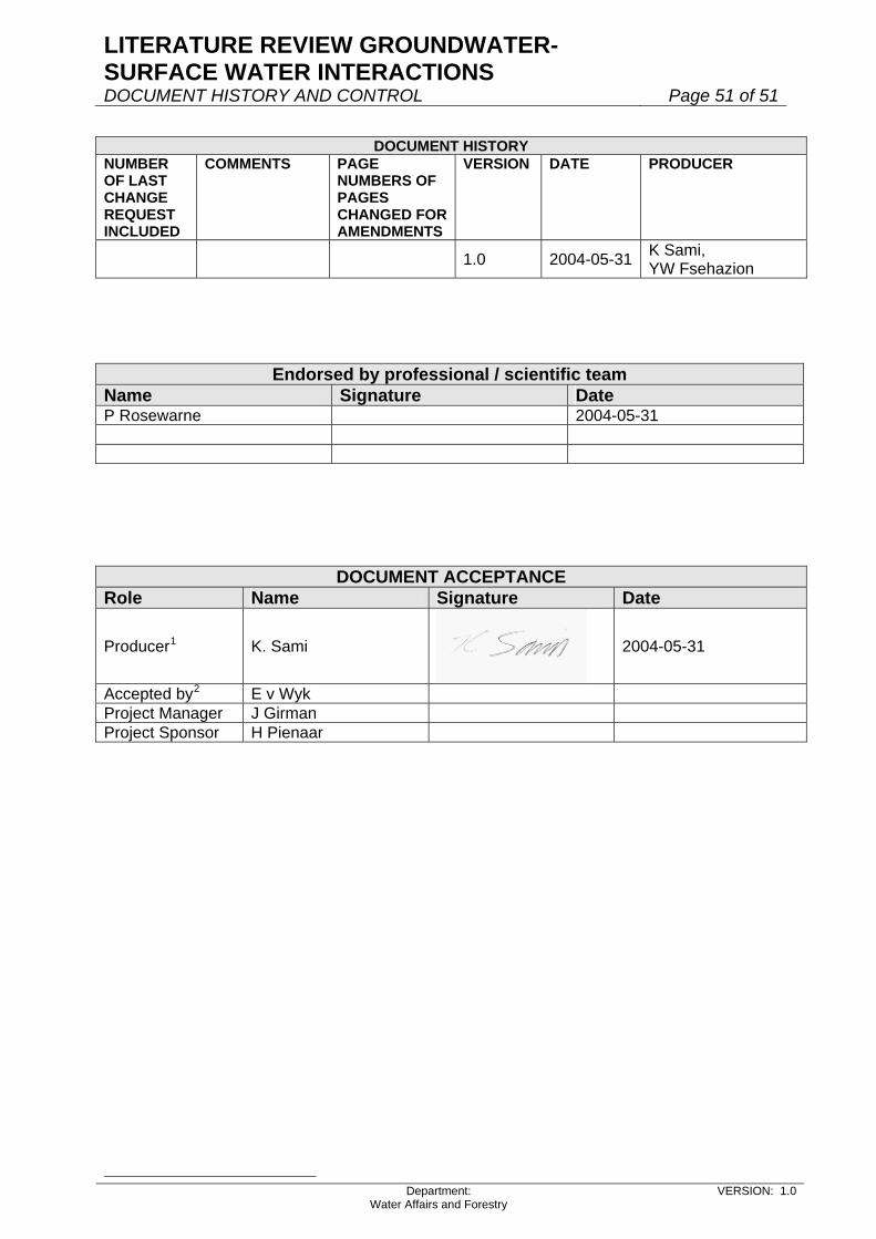
LITERATURE REVIEW GROUNDWATER-SURFACE WATER INTERACTIONS
DOCUMENT HISTORY AND CONTROL Page 51 of 51
Department: Water Affairs and Forestry
VERSION: 1.0
DOCUMENT HISTORY
NUMBER OF LAST CHANGE REQUEST INCLUDED
COMMENTS PAGE NUMBERS OF PAGES CHANGED FOR AMENDMENTS
VERSION DATE PRODUCER
K Sami, 1.0 2004-05-31 YW Fsehazion
Endorsed by professional / scientific team Name Signature Date P Rosewarne 2004-05-31
DOCUMENT ACCEPTANCE Role Name Signature Date
Producer1 K. Sami
2004-05-31
Accepted by2 E v Wyk Project Manager J Girman Project Sponsor H Pienaar