Harvard | Business | School

The Behavioral Finance and Financial Stabilities Project

Working Paper 2016-01

Project on Behavioral Finance and Financial Stability

Sergey Chernenko

Adi Sunderam

Liquidity Transformation in Asset Management:

Evidence from the Cash Holdings of Mutual Funds

Liquidity Transformation in Asset Management:

Evidence from the Cash Holdings of Mutual Funds*

Sergey Chernenko sergey.chernenko@fisher.osu.edu

The Ohio State University

Adi Sunderam asunderam@hbs.edu

Harvard University and NBER

July 15, 2016

Abstract

We study liquidity transformation in mutual funds using a novel data set on their cash holdings.

To provide investors with claims that are more liquid than the underlying assets, funds engage in

substantial liquidity management. Specifically, they hold substantial amounts of cash, which they

use to accommodate inflows and outflows rather than transacting in the underlying portfolio

assets. This is particularly true for funds with illiquid assets and at times of low market liquidity.

We provide evidence suggesting that mutual funds’ cash holdings are not large enough to fully

mitigate price impact externalities created by the liquidity transformation they engage in.

* We thank Jules van Binsbergen, Jaewon Choi, Lauren Cohen, Robin Greenwood, Johan Hombert, Marcin Kacperczyk, Xuewen Liu, Alexi Savov, Jeremy Stein, René Stulz, Robert Turley, Jeff Wang, Zhi Wang, Michael Weisbach, Yao Zeng, and seminar participants at the 3rd Annual Conference on Financial Market Regulation, Adam Smith Conference, Duke/UNC Asset Pricing Conference, Federal Reserve Bank of New York, NBER New Developments in Long-Term Asset Management Conference, NBER Risks of Financial Institutions Conference, Ohio State University, Risk Management Conference Mont Tremblant, Texas A&M, University of Illinois Urbana-Champaign, and University of Massachusetts at Amherst for helpful comments and suggestions. Yuan He and Mike Dong provided excellent research assistance.

1

I. Introduction

Liquidity transformation – the creation of liquid claims that are backed by illiquid assets

– is a key function of many financial intermediaries. A long literature, starting with Diamond and

Dybvig (1983) and Gorton and Pennacchi (1990), argues, for example, that the purpose of banks

is to provide investors with highly liquid demand deposits while financing illiquid, information

intensive loans. Liquidity transformation is also an important function of the system of market-

based intermediaries known as the shadow banking system, as argued by Gorton and Metrick

(2010), Kacperczyk and Schnabl (2010), Krishnamurthy and Vissing-Jorgenson (2015), Moreira

and Savov (2016), and Nagel (2016).

Through open-ending – allowing investors to withdraw capital at short notice –

traditional asset managers provide liquidity services that are similar to banks and shadow banks.

For example, though they may invest in illiquid assets such as corporate bonds, bank loans, and

emerging market stocks, open-end mutual funds have liquid liabilities. Specifically, mutual funds

allow investors to redeem any number of shares at the fund’s end-of-day net asset value (NAV),

effectively pooling liquidation costs across investors. In contrast, investors who directly hold the

underlying investments bear their own liquidation costs when selling those assets.

Can liquidity transformation by asset managers cause financial stability problems? This

question has been the subject of a vigorous debate among academics, practitioners, and

regulators (e.g., Goldstein et al, 2015; International Monetary Fund, 2015; Financial Stability

Oversight Council, 2014; Feroli et al, 2014; Chen, Goldstein, and Jiang, 2010). A key concern on

one side of the debate is that liquidity transformation increases the scope for fire sales.

Redemptions from an open-end fund can force sales of illiquid assets, depressing asset prices and

thereby stimulating further redemptions and fire sales. Motivated by such concerns, the

Securities and Exchange Commission (SEC) has recently proposed new rules to promote more

effective liquidity risk management by mutual funds (SEC, 2015).

On the opposite side of the debate are two main arguments. First, many contend that asset

managers are essentially a veil, simply transacting in the underlying equities and bonds on behalf

2

of investors without performing much liquidity transformation (Investment Company Institute,

2015). Second, others argue that asset managers are well aware of the risks of fire sales and take

steps to manage their liquidity needs (Independent Directors Council, 2016; Investment

Company Institute, 2016).

A key empirical challenge in this debate is that it is difficult to measure liquidity

transformation for asset managers. For banks and shadow banks, maturity mismatch – the

difference in maturity between assets and liabilities – provides a reasonable measure of liquidity

transformation. While investors can withdraw unlimited quantities of deposits without any price

impact, bank loans cannot be traded before maturity without creating substantial price impact.

For asset managers, however, there is no comparable measure. Their assets are typically

tradeable securities, though with varying levels of liquidity. Furthermore, some price impact can

be passed on to investors because they own claims whose value is not fixed. Nevertheless, asset

managers perform some amount of liquidity transformation because their ability to pool trades

and space transactions over time flattens the price-quantity schedule faced by their investors.

In this paper, we use the cash holdings of open-end mutual funds that invest in equities

and long-term corporate bonds as a window into the liquidity transformation activities of asset

managers.1 Our key insight is that the way mutual funds manage their own liquidity to provide

the benefits of open-ending to investors sheds light on how much liquidity transformation funds

are performing. A fund acting as a pure pass-through, simply buying and selling the underlying

assets on behalf of its investors, has little need for cash holdings to manage its liquidity. In

contrast, a fund performing substantial liquidity transformation will seek to use cash holdings to

mitigate the costs associated with providing investors with claims that are more liquid than the

underlying assets. This revealed preference argument suggests that funds’ cash management

practices can be used to measure their liquidity transformation.

1 Because we focus on the mismatch in liquidity between fund assets and liabilities, we exclude money market mutual funds, closed-end funds, index funds, ETFs, and short-term bond mutual funds from our analysis.

3

Two features of the mutual fund industry make it a good laboratory for studying liquidity

transformation by asset managers. First, mutual funds account for a large fraction of the overall

asset management industry. As of 2015Q1, mutual funds had aggregate assets of $12.9 trillion

and held 20.5% of corporate equities and 20.6% of corporate and foreign bonds.2 Second, while

other asset managers have some ability to restrict investor redemptions, most mutual funds are

completely open-ended, creating significant scope for liquidity transformation.

We study mutual fund liquidity management using a novel data set on the cash holdings

of equity and long-term corporate bond funds collected from the SEC form N-SAR filings.

Importantly, our data set covers holdings of both cash and cash substitutes such as money market

mutual fund shares. In recent years, cash substitutes have become an increasingly important

source of liquidity for asset managers. The IMF estimates that asset managers as a whole held

about $2 trillion of cash and cash substitutes in 2013 (Pozsar, 2013). This is approximately the

same amount as US corporations (Bates et al., 2009). Approximately 37% of asset manager cash

holdings is in the form of cash substitutes (Pozsar, 2013). Fig. 1 shows that a similar pattern

holds for the equity and long-term bond mutual funds in our data set. By 2014, they held $600

billion of cash and cash substitutes, with nearly 50% taking the form of cash substitutes.

We present four main results on mutual fund liquidity management, all showing that

mutual funds do not simply act as pass-throughs. Instead, consistent with the idea that mutual

funds perform a significant amount of liquidity transformation, funds use holdings of cash to

actively manage their liquidity provision and to reduce their impact on the prices of the

underlying assets. Our first main result is that, rather than transacting in equities and bonds,

mutual funds use cash to accommodate inflows and outflows. Funds build up cash positions

when they receive inflows and draw down cash when they suffer outflows. The magnitudes are

economically significant. For each dollar of inflows or outflows in a given month, 23 to 33 cents

2 Federal Reserve Flow of Funds. These numbers do not include the assets of money market mutual funds.

4

of that flow is accommodated through changes in cash rather than through trading in the fund’s

portfolio securities. This impact of flows on cash balances lasts for multiple months.

Second, asset liquidity affects the propensity of funds to use cash holdings to manage

fund flows. In the cross section, funds with illiquid assets are more aggressive in using cash to

meet inflows and outflows. A one-standard deviation increase in asset illiquidity is associated

with a 20-30% increase in the fraction of fund flows accommodated through changes in cash. We

find similar evidence in the time series: during periods of low aggregate market liquidity, funds

accommodate a larger fraction of fund flows with cash. These results would not obtain if funds

were simply a veil, trading on behalf of their investors. Instead, our results are consistent with

the idea that mutual funds perform a significant amount of liquidity transformation, with their

cash holdings playing a critical role.

Third, we show that funds that perform more liquidity transformation hold significantly

more cash. Asset illiquidity, the volatility of fund flows, and their interaction are the key

determinants of how much liquidity transformation a given fund engages in, and we find that all

three variables are strongly related to cash holdings. For equity funds, for example, a one-

standard deviation increase in asset illiquidity (flow volatility) is associated with a 1.0 (0.4)

percentage points higher cash-to-assets ratio. Furthermore, the interaction of asset illiquidity and

flow volatility is positive and statistically significant, indicating that funds that invest in illiquid

assets and provide investors with ample liquidity have particularly high cash-to-assets ratios. The

magnitude of these effects is large. For the funds with the most liquid assets in our sample, cash

holdings do not vary with flow volatility, indicating that these funds are close to the frictionless

null. However, the average fund is quite far from this frictionless benchmark. Overall, because

they use cash to manage liquidity, mutual funds hold large aggregate amounts of cash.

Are these cash holdings large enough to fully mitigate any price impact externalities that

funds may exert on other market participants? We provide two pieces of suggestive evidence that

they are not. The first piece of evidence arises from the intuition that a monopolist internalizes its

price impact. We show that funds that hold a larger fraction of the outstanding amount of the

5

assets they invest in tend to hold more cash. This finding is consistent with such funds more fully

internalizing the price impact of their trading in the securities they hold. Our second piece of

evidence is at the fund family level. We show that funds that have significant holdings overlap

with other funds in the same family hold more cash. This finding is consistent with the idea that

these funds are more cautious about exerting price impact when it may adversely affect other

funds in the family.

We also explore the extent to which funds use alternative liquidity management tools,

including redemption restrictions, credit lines, and interfund lending programs in lieu of cash.

Our evidence indicates that these alternative tools are imperfect substitutes for cash and that cash

is the key tool funds use for liquidity management. These results validate our insight that cash

holdings are a good measure of a fund’s liquidity transformation activities.

In summary, our analysis highlights three key properties of liquidity transformation in

asset management. First, it is economically significant. Mutual funds are not a veil, simply

transacting in bonds and equities on behalf of their investors. Instead, funds have substantial cash

holdings and use them to accommodate inflows and outflows, even at horizons of a few months.

Second, liquidity transformation in asset management is highly dependent on liquidity

provision by the traditional and shadow banking sectors. In order to provide liquidity to their

investors, mutual funds must hold substantial amounts of cash, bank deposits, and money market

mutual fund shares. These holdings do not decrease much with fund size, suggesting that

economies of scale in liquidity provision are weak.

Third, despite their size, the cash holdings of mutual funds are not sufficiently large to

completely mitigate the price impact externalities created by funds’ liquidity transformation

activities. Our evidence suggests that funds do not fully internalize the effect that providing

investors with daily liquidity has on the prices of the underlying securities.

Our paper is related to several strands of the literature. First, there is a small but growing

literature studying the potential for liquidity transformation among mutual funds to generate run-

6

like dynamics, including Chen, Goldstein, and Jiang (2010), Feroli et al (2014), Goldstein, Jiang,

and Ng (2015), Wang (2015), and Zeng (2015). Second, there is a large theoretical and empirical

literature studying fire sales in debt and equity markets, including Shleifer and Vishny (1992),

Shleifer and Vishny (1997), Coval and Stafford (2007), Ellul, Jotikasthira and Lundblad (2011),

Greenwood and Thesmar (2011), and Merrill et al (2012).3 Our results show how mutual funds

use cash holdings to manage the risk of fire sales created by their liquidity transformation

activities and suggest that they may not hold enough cash to fully mitigate fire sale externalities.

Our paper is also related to the large literature on liquidity transformation in banks,

including recent empirical work measuring liquidity creation in banks such as Berger and

Bouwman (2009) and Cornett et al (2011). It is also related to the literature on instabilities in

shadow banking, including Gorton and Metrick (2012), Stein (2012), Kacperczyk and Schnabl

(2013), Krishnamurthy, Nagel, and Orlov (2014), Chernenko and Sunderam (2014), and

Schmidt, Timmerman, and Wermers (2016).

Finally, we contribute to a small but growing literature on the determinants and effects of

mutual fund cash holdings, including Yan (2006), Simutin (2014), and Hanouna, Novak, Riley,

and Stahel (2015). While this literature focuses primarily on funds’ market timing ability and the

impact cash holdings have on returns, we use cash holdings as a measure of liquidity

transformation. We empirically validate this measure and use it to argue that mutual funds

perform a substantial amount of liquidity transformation. In addition, we use the measure to

examine the extent to which funds internalize the price impact they exert on security prices.

The remainder of the paper is organized as follows. Section II presents a simple

framework that demonstrates the link between liquidity transformation and optimal cash

3 In addition, there is a broader literature on debt and equity market liquidity, including Roll (1984), Amihud and Mendelsohn (1986), Chordia, Roll, and Subrahmanyam (2001), Amihud (2002), Longstaff (2004), Acharya and Pedersen (2005), Bao, Pan, and Wang (2011), Dick-Nielsen, Feldhütter, and Lando (2012), Feldhütter (2012), and many others. Our results demonstrate that asset managers perform liquidity transformation in a manner similar to banks, providing investors with liquid claims while holding less liquid securities, which they must ultimately trade in the debt and equity markets.

7

holdings. Section III describes the data. Section IV presents our main results on cash

management by mutual funds. Section V provides evidence on how much of their price impact

individual mutual funds internalize. Section VI discusses alternative liquidity management tools

and argues that they play a secondary role relative to cash holdings, and Section VII concludes.

II. Framework

Throughout the paper, we use liquidity transformation to mean that the price-quantity

schedule faced by a fund investor in buying or selling fund shares is different from what it would

be if the investor directly traded in the underlying assets.

There are three main ways mutual funds can perform liquidity transformation. First,

funds allow investors to buy and sell unlimited quantities at the end-of-day NAV. In contrast,

individual investors trading by themselves would create more price impact if they traded larger

quantities. Second, funds can use cash buffers to pool investor buy and sell orders that may be

asynchronous. Essentially, if some fraction of fund flows are temporary and will be offset in the

near future, the fund can use cash buffers to net these flows. This is analogous to the way

diversification across depositors allows banks to hold illiquid assets, as in Diamond and Dybvig

(1983). Individual investors trading for themselves in a market would achieve this only if they

traded simultaneously. Third, funds can use cash buffers to mitigate price impact when trading in

the underlying assets. If price impact is increasing in the quantity traded but temporary, then

funds can use cash buffers to spread out their trades across time in order to reduce their price

impact. Similarly, if market liquidity varies over time, funds can use cash buffers to allocate their

trades to periods with low price impact.

A. Cash management

To help fix ideas, we begin by outlining the logic of our empirical tests. In the Internet

Appendix, we present a simple static model that formally derives many of these predictions. We

consider a fund charged with managing a pool of risky, illiquid assets to outperform a benchmark

while providing regular liquidity to its investors. Our predictions are based on the idea that an

8

optimizing fund will use cash buffers to help meet this mandate. The key tradeoff the fund faces

is that cash buffers help reduce price impact when trading the illiquid assets, but they have a

carrying cost because they increase tracking error relative to the benchmark.

We conduct three sets of empirical tests. The first one involves fund cash management

practices.

Prediction 1. A fund’s propensity to use cash to accommodate flows is a measure of its

liquidity transformation.

The logic here is that if fund assets were perfectly liquid, the fund would have no need to use

cash. It could always trade in the underlying assets immediately and frictionlessly, so holding

cash buffers would only increase the fund’s tracking error. On the other hand, if the fund is

performing liquidity transformation, it can use its cash buffers to mitigate the price impact

associated with trading in the underlying. The same logic suggests that the strength of this cash

management motive varies with the illiquidity of the underlying assets.

Prediction 2. In both the cross section and the time series, funds performing more liquidity

transformation should more aggressively use cash to accommodate flows.

The more illiquid fund assets are, the longer the fund will take to accommodate flows. The

reason is that when assets are more illiquid, costs of delay become smaller relative to the price

impact of trading. Similarly, when assets are more illiquid, the value of waiting for offsetting

flows increases. Assets can be more illiquid either because of the fund’s choice of assets (e.g.,

small cap versus large cap stocks) or because of aggregate variation in market liquidity.

B. Cash holdings for a single fund

Our next set of empirical tests involves the level of cash holdings.

Prediction 3. The level of cash holdings is a measure of equilibrium liquidity transformation.

This may seem somewhat counterintuitive, as all else equal, more cash reduces the

amount of liquidity transformation the fund is doing. In the limit, a fund holding only cash does

9

not perform any liquidity transformation. However, the prediction is about funds’ optimal

equilibrium behavior. The logic is that funds trade off the incremental carrying costs of having

more cash against the expected incremental trading costs associated with having less cash.

It follows from the fund’s trade off that optimal cash reserves are increasing in the fund’s

expected trading costs. Intuitively, if the fund chooses to hold more cash, it is choosing to pay

higher carrying costs. This is optimal only if the fund faces higher expected trading costs.

Furthermore, a fund with higher expected trading costs will not hold enough cash to fully offset

those costs. The fund always bears the incremental carrying costs but enjoys reduced trading

costs only when there are large outflows. Thus, a fund’s optimal cash holdings are increasing in

the amount of liquidity transformation it performs.

Prediction 4. If cash holdings are driven by liquidity transformation, they should increase with

asset illiquidity, the volatility of fund flows, and the interaction of the two.

Liquidity transformation is driven by the intersection of investor behavior and asset

illiquidity. Funds with more volatile flows are effectively providing greater liquidity services to

their investors. Similarly, if the fund’s assets are more illiquid, it is providing greater liquidity

services to its investors. These two effects interact: the more illiquid the assets, the stronger the

relationship between cash-to-assets ratios and flow volatility.

C. Internalizing price impact

Our third set of predictions involves the extent to which fund cash holdings are high enough

to prevent funds from exerting price impact externalities on one another. We consider the

alternative, where the level of cash holdings is picked by a planner minimizing total costs

(carrying costs of cash plus trading costs incurred by funds) borne by all funds.

Prediction 5. A planner coordinating the level of cash holdings among funds would choose a

higher level than the level chosen in the private market equilibrium.

This is the analog of a leverage or fire sale externality as in Shleifer and Vishny (1992) or

Stein (2012). In the private market equilibrium, each individual fund treats other funds’ reserve

10

policies as fixed when choosing its own reserves. An individual fund does not internalize this

positive effect its cash holdings have on the trading costs faced by the other funds. Specifically,

when an individual fund has more cash, it needs to trade less and thus creates less price impact.

This benefits other funds that need to trade in the same direction as the individual fund. In

contrast, the planner internalizes the fact that high reserves benefit all funds through lower

liquidation costs.

Note that there is no welfare statement here. For there to be a social loss from low cash

holdings in general equilibrium, the liquidation costs to the funds must not simply be a transfer

to an outside liquidity provider. Our prediction is simply that coordination among funds would

lead to higher cash holdings.

A corollary that follows from this logic is that a monopolist in a particular security

internalizes its price impact, particularly if that security is illiquid. The externality that makes

private market cash holdings lower than what a planner would choose arises because funds take

into account how cash holdings mitigate their own price impact but not how that price impact

affects other funds. Of course, if one fund owns the whole market, there is no externality. When

a monopolist creates price impact through trading, it is the only fund that suffers because it is the

only one that holds the security. Put differently, the monopolist and the planner solve the same

problem: minimizing the sum of cash carrying costs and trading costs in the security.

Generalizing this intuition, the higher is the fraction of the underlying assets owned by a given

fund, the more will the fund internalize its price impact.

Corollary: Funds that own a larger fraction of their portfolio assets more fully internalize

their price impact and therefore hold more cash reserves.

III. Data

A. Cash holdings

We combine novel data on the cash holdings of mutual funds with several other data sets.

Our primary data comes from the SEC form N-SAR filings. These forms are filed semi-annually

11

by all mutual funds and provide data on asset composition, including holdings of cash and cash

substitutes. Specifically, we measure holdings of cash and cash substitutes as the sum of cash

(item 74A), repurchase agreements (74B), short-term debt securities other than repurchase

agreements (74C), and other investments (74I). Short-term debt securities have remaining

maturities of less than a year and consist mostly of US Treasury Bills and commercial paper. The

demarcation between cash and other assets is less clear for bond funds than for equity funds

because bond funds may hold short-term debt for both liquidity management and pure

investment reasons. We focus on long-term bond funds for this reason, but our measures of cash

are still likely to be noisier for bond funds than equity funds.

The other investments category (74I) consists mostly of investments in money market

mutual funds (MMMFs), other mutual funds, loan participations, and physical commodities.

Using hand-collected data, we have examined the composition of the other investments category

for a random sample of 320 funds for which other investments accounted for at least 10% of total

net assets. The mean and median fractions of MMMFs in other investments were 75% and

100%. Holdings of other mutual funds accounted for most of the remaining value of other

investments. We use our security-level holdings data, described below, to subtract holdings of

long-term mutual funds from other investments. Otherwise, we treat the other investments

category as consisting entirely of MMMFs. This should only introduce measurement error into

our dependent variable and potentially inflate our standard errors.4

Our dependent variable is thus the sum of cash and cash equivalents scaled by TNA (item

74T). We winsorize this cash ratio at the 1st and 99th percentiles.

4 The CRSP Mutual Fund Database includes a variable called per_cash that is supposed to report the fraction of the fund’s portfolio invested in cash and equivalents. This variable appears to be a rather noisy proxy for the cash-to-assets ratio. Aggregate cash holdings of all long-term mutual funds in CRSP track aggregate holdings of liquid assets of long-term mutual funds as reported by the Investment Company Institute (ICI) until 2007, but the relationship breaks down after that. By 2014, there is a gap of more than $400 billion, or more than 50% of the aggregate cash holdings reported by ICI. At a more granular level, we calculated cash holdings from the bottom up using security-level data from the SEC form N-CSR for a random sample of 100 funds. The correlation between the true value of the cash-to-assets ratio computed using N-CSR data and our N-SAR based proxy is 0.75. The correlation between the true value and CRSP is only 0.40.

12

In addition to data on asset composition, form N-SAR contains data on fund flows and

investment practices. Gross and net fund flows for each month since the last semi-annual filing

are reported in item 28. Item 70 reports indicators for whether the fund uses various types of

derivatives, borrows, lends out it securities, or engages in short sales.5

B. Link to CRSP mutual fund database

For additional fund characteristics such as investment objective, fraction of institutional

share classes, and holdings liquidity, we link our N-SAR data to the CRSP Mutual Fund

Database. Using a name-matching algorithm, we can match the majority of funds in N-SAR to

CRSP.6 We match more than 70% of all fund-time observations in N-SAR to CRSP. In dollar

terms, we match more than 80% of all assets.

After linking our data to CRSP, we apply the following screens to our sample of funds.

We focus on open-end funds and exclude exchange-traded funds (ETFs),7 small business

investment companies (SBIC), unit investment trusts (UIT), variable annuities, funds of funds,8

and money market mutual funds. In addition, we exclude observations with zero assets according

to N-SAR and those for which the financial statements do not cover a regular 6- or 12-month

5 Almazan et al (2004) also use form N-SAR’s investment practices data. 6 Our procedure takes advantage of the structure of fund names in CRSP. The full fund name in CRSP is generally of the form “trust name: fund name; share class.” For example, “Vanguard Index Funds: Vanguard 500 Index Fund; Admiral Shares.” The first piece, “Vanguard Index Funds,” is the name of the legal trust that offers Vanguard 500 Index Fund as well as a number of other funds. Vanguard Index Funds is the legal entity that files on behalf of Vanguard 500 Index Fund with the SEC. The second piece, “Vanguard 500 Index Fund,” is the name of the fund itself. The final piece, “Admiral Shares,” indicates different share classes that are claims on the same portfolio but that offer different bundles of fees, minimum investment requirements, sales loads, and other restrictions. 7 ETFs operate a very different model of liquidity transformation. They rely on investors to provide liquidity in the secondary market for the fund’s share and on authorized participants (APs) to maintain parity between the market price of the fund’s shares and their NAV. In untabulated results, we find that ETFs hold significantly less cash and that to the extent that they do hold more than a token amount of cash, it is almost entirely due to securities lending and derivatives trading. 8 SBICs, UITs, and open-end funds are identified based on N-SAR items 5, 6, and 27. ETFs are identified based on the ETF dummy in CRSP or fund name including the words ETF, exchange-traded, iShares, or PowerShares. Variable annuities are identified based on N-SAR item 58. We use security-level data from CRSP and Morningstar to calculate the share of the portfolio invested in other mutual funds. Funds that, on average, invest more than 80% of their portfolio in other funds are considered to be funds of funds.

13

reporting period. As we discuss below, we are able to measure asset liquidity for domestic equity

funds, identified using CRSP objective codes starting with ED, and for long-term corporate bond

funds.9 To further make sure that we can accurately measure fund flow volatility and asset

liquidity, we focus on funds with at least $100 million in assets. Finally, we exclude index funds

for two reasons. First, index funds are likely to have higher carrying costs (i.e., costs of tracking

error) than other funds. Thus, for index funds, cash holdings are likely to be lower and less

sensitive to asset liquidity and fund flow volatility, and therefore a noisier measure of liquidity

transformation. Second, index funds largely track the most liquid securities, so there is little

variation in asset liquidity for us to analyze among them.

C. Asset liquidity

We use holdings data from the CRSP Mutual Fund Database to measure the liquidity of

equity mutual fund holdings.10 These data start in 2003. Following Chen, Goldstein, and Jiang

(2010), we construct the square root version of the Amihud (2002) liquidity measure for each

stock. We then aggregate up to the fund-quarter level, taking the value-weighted average of

individual stock liquidity.

For bond funds, we use monthly holdings data from Morningstar, which covers the

2002Q2-2012Q2 period. Following Dick-Nielsen, Feldhütter, and Lando (2012) we measure

liquidity of individual bonds as λ, the equal-weighted average of four other liquidity measures:

Amihud, Imputed Roundtrip Cost (IRC) of Feldhutter (2012), Amihud risk, and IRC risk.11 The

latter two are the standard deviations of the daily values of Amihud and IRC within a given

quarter. Once we have the λ measure for each bond, we aggregate up to the fund level, taking the

value-weighted average of individual bond liquidity.

9 Corporate bond funds are defined as funds that have Lipper objective codes A, BBB, HY, IID, MSI, and MSI and that invest more than 50% of their portfolio in intermediate and long-term corporate bonds (NSAR item 62P). 10 In unreported analyses, we obtain very similar results when we use Thomson Reuters Mutual Funds Holdings data. 11 We are grateful to Peter Feldhütter for sharing his code with us.

14

D. Summary statistics

Our final data set is a semi-annual fund-level panel that combines the N-SAR data with

additional fund information from CRSP and data on asset liquidity from CRSP and Morningstar.

Throughout the paper, we conduct our analysis at the fund-half year level.

The sample periods are determined by the availability of holdings data in CRSP and

Morningstar and of bond transaction data in TRACE. For equity funds, the sample period is

January 2003 – December 2014. For bond funds, it is September 2002 – June 2012.

Table 1 reports basic summary statistics for funds in our data, splitting them into equity

versus bond funds. Our sample of equity funds consists of about 22,000 observations. Our

sample of bond funds is much smaller, only about one eight the size of the equity fund sample.12

Equity and bond funds are broadly comparable in size with median TNA of $500 – 600 million

and mean TNA of $2.1 – 2.5 billion.

Bond funds tend to hold more cash. The median bond fund has a cash-to-assets ratio of

5.3%, while the median equity fund has a cash-to-assets ratio of 4.4%. Bond funds have

significantly higher turnover.13 The volatility of fund flows is comparable for bond and equity

funds, averaging approximately 9-10% per year. Institutional ownership is also similar. Except

for securities lending, bond funds are somewhat more likely than equity funds to engage in

various sophisticated investment practices such as trading options and futures and shorting.

Appendix Table A1 gives formal definitions for the construction of all variables used in

the analysis.

12 The number of bond funds in our sample is significantly smaller than the number of equity funds because we focus on bond funds that invest at least 50% of their portfolio in corporate bonds. 13 Higher turnover of bond funds is in part due to a) bond maturities being treated as sales and b) trading in the to-be-announced market for agency MBS.

15

IV. Results

We now present our main results. We start by showing that cash holdings play an

economically significant role in how mutual funds manage their liquidity to meet inflows and

outflows. We then study the determinants of cash holdings, showing that cash holdings are

strongly related to asset liquidity and volatility of fund flows. It is worth noting that for much of

the analysis, we are documenting endogenous relationships. Fund characteristics, investor

behavior, and cash holdings are all jointly determined, and our results trace out the endogenous

relationships between them.14

A. Liquidity management through cash holdings

We begin by examining Prediction 1 from Section II. We show that cash holdings play an

important role in the way mutual funds manage inflows and outflows. In Table 2, we estimate

regressions of the change in a fund’s cash holdings over the last six months on the net flows it

received during each of those six months:

ΔCashi ,t−6→t =αobj (i ),t +β0Flowsi ,t + ...+β5Flowsi ,t−5 +εi ,t . (6)

Fund flows are winsorized at the 5th and 95th percentiles. In Appendix Table A2, we show that

we obtain similar results winsorizing at the 1st and 99th percentiles. All specifications include

Lipper objective code cross time (half-year) fixed effects, indicating that the results are not

driven by relationships between flows and cash holdings in particular fund objectives.

We first examine the results for equity funds. In the first column of Table 2, the

dependent variable is the change in cash holdings over the last six months as a fraction of net

assets six months ago: ΔCashi ,t−6→t /TNAi ,t−6 . In the first column, the coefficient β0 = 0.23 is large

and highly statistically significant. Since flows are scaled by the same denominator – assets six 14 In most cases, endogeneity should lead to coefficients that are smaller in magnitude. For instance, Chen, Goldstein, and Jiang (2010) argue that higher cash holdings should endogenously lower the volatility of fund flows because investors are less worried about fire sales. This should weaken the relationship between cash and fund flow volatility relative to the case where fund flow volatility is exogenous.

16

months ago – as the dependent variable, the coefficients can be interpreted as dollars. Thus, β0 =

0.23 indicates that a dollar of outflows during month t decreases cash holdings by 23 cents.

Similarly, a dollar of inflows increases cash holdings by 23 cents. The other 77 cents are met by

transacting in the fund’s holdings of equities.15 In untabulated results, when we run regressions

separating inflows and outflows, we find that funds respond relatively symmetrically to them.

This is consistent with the idea that funds care about the price pressure they exert on the

underlying assets when both buying and selling.

The coefficient β0 shows that an economically significant portion of flows is

accommodated through cash holdings. Even though equities are quite liquid, and a month is a

relatively long period, 23% of flows at a monthly horizon are accommodated through changes in

cash holdings. Presumably, at higher frequencies (e.g., daily or weekly), cash plays an even more

important role. The remaining coefficients show that the effect of fund flows on cash holdings

declines over time. However, even fund flows in month t-4 still have a detectable effect on cash

holdings at time t.

In the second column of Table 2, the dependent variable is the change in the fund’s cash-

to-assets ratio:

ΔCashTNA

⎛

⎝⎜

⎞

⎠⎟i ,t

=CashTNA

⎛

⎝⎜

⎞

⎠⎟i ,t

−CashTNA

⎛

⎝⎜

⎞

⎠⎟i ,t−6

.

These regressions show that funds are not simply responding to flows by scaling their portfolios

up and down. The overall composition of the portfolio is changing, becoming more cash-heavy

when the fund receives inflows and less cash-heavy when the fund suffers outflows.

The coefficient β0 = 0.087 is statistically and economically significant. Flows equal to

100% of assets increase the fund’s cash-to-assets ratio by 8.7% (percentage points). For

reference, the standard deviation of fund flows is 9%. The coefficients here are likely to be

15 These results are broadly consistent with Edelen (1999), who finds that a dollar of fund flows is associated with about 70 cents in trading activity.

17

biased down because of the performance-flow relationship. If a fund has strong returns between

month t-6 and month t, it is likely to receive inflows, but its cash-to-assets ratio at time t will be

depressed because high returns inflate assets at time t.

The last two columns of Table 2 report analogous results for bond funds. The coefficients

are again large and statistically significant, and the economic magnitudes are larger. Specifically,

in column (3), the coefficient β0 = 0.33 indicates that one dollar of outflows in month t decreases

cash holdings by 33 cents. Similarly, in column (4), the coefficient β0 = 0.124 indicates that

flows equal to 100% of assets increase the fund’s cash-to-assets ratio by 12.4% (percentage

points). The larger magnitudes we find for bond funds are consistent with bonds being less liquid

than equities. Because funds face larger price impact when trading bonds, they accommodate a

larger share of fund flows through changes in cash.

B. Effect of asset liquidity and market illiquidity

We next turn to Prediction 2 from Section II, examining how illiquidity affects funds’

propensity to use cash to manage inflows and outflows in both the cross section and the time

series. Panel A of Table 3 estimates specifications that allow cash management practices to differ

across the cross section of funds based on the illiquidity of their assets. Specifically, we estimate:

ΔCashi ,t−6→t =αobj (i ),t +β1Flowsi ,t−2→t +β2Flowsi ,t−2→t × Illiqi ,t−6

+β3Flowsi ,t−5→t−3 +β4Flowsi ,t−5→t−3 × Illiqi ,t−6 +β5Illiqi ,t−6 +εi ,t . (7)

For compactness, we aggregate flows into quarters, i.e., those from month t-5 to t-3 and month t-

2 to t.16 We interact each of these quarterly flows with the lagged values of holdings illiquidity.

Thus, the specification asks: given the illiquidity of the holdings that a fund had two quarters

ago, how did it respond to fund flows during the last two quarters?

For equity funds studied in the first two columns, illiquidity is measured as the square

root version of the Amihud (2002) measure. In the first column, the dependent variable is the 16 Interacting monthly flows with asset illiquidity generates somewhat stronger results for more recent fund flows.

18

change in cash holdings over the last six months as a fraction of assets six months ago:

ΔCashi ,t−6→t /TNAi ,t−6 . We standardize the illiquidity variables so that their coefficients can be

interpreted as the effect of a one-standard deviation change in asset illiquidity. Again, all

specifications have Lipper objective cross time fixed effects. The first column of Table 3 Panel A

shows that for the average equity fund, one dollar of flows over months t-2 to t changes cash

holdings by β1 = 17 cents. For a fund with assets one standard deviation more illiquid than the

average fund, the same dollar of flows changes cash holdings by β1 + β2 = 21 cents, a 21% larger

effect. In the second column, the dependent variable is the change in the fund’s cash-to-assets

ratio. Once again, fund flows over the last three months have a larger effect on funds with more

illiquid assets.

The last two columns of Table 3 Panel A report analogous results for bond funds. The

magnitudes are similar. Column (3) shows that for the average bond fund, one dollar of flows

over months t-2 to t changes cash holdings by β1 = 15 cents. For a fund with assets one standard

deviation more illiquid than the average fund, the same dollar of flows changes cash holdings by

β1 + β2 = 19 cents, a 28% larger effect. However, in column (4), neither the coefficient on flows

nor its interaction with asset illiquidity is statistically significant.

In Panel B, we next turn to time variation in how funds manage their liquidity. When

markets for the underlying securities are less liquid, funds should have a higher propensity to

accommodate flows through changes in cash. Table 3 Panel B estimates specifications of the

form:

ΔCashi,t−6→t =αobj(i),t +β1Flowsi,t−2→t +β2Flowsi,t−2→t × LowAggLiqi,t−2→t+β3Flowsi,t−5→t−3+β4Flowsi,t−5→t−3× LowAggLiqi,t−5→t−3+εi,t .

(8)

We measure aggregate market liquidity during separate quarters and then define the bottom

19

tercile as periods of low aggregate market liquidity. For equity funds, our measure of aggregate

market liquidity is the Pastor and Stambaugh (2003) measure.17

The first column of Table 3 Panel B shows that for the average half-year, one dollar of

fund flows during months t-2 to t changes cash balances by β1 = 16 cents. When aggregate

market liquidity is low, the same dollar of flows changes cash balances by β1 + β2 = 21 cents,

30% more. In the second column, the dependent variable is the change in the fund’s cash-to-

assets ratio. Here again, we see evidence that cash-to-assets ratios are more sensitive to fund

flows when aggregate market liquidity is low.

The last two columns of Table 3 Panel B turn to bond funds. There is less agreement in

the literature over the appropriate way to measure the liquidity of the aggregate bond market. We

use the average of Dick-Nielsen, Feldhütter, and Lando (2012) lambda across all US-traded

corporate bonds.18 Column (3) of Panel B shows that one dollar of fund flows during months t-2

to t changes cash balances by β1 = 10 cents. When aggregate market liquidity is low, the same

dollar of flows changes cash balances by β1 + β2 = 23 cents, or over 100% more. However, in

column (4), neither the coefficient on flows nor its interaction with market liquidity is

statistically significant. We have less power to detect the effect of aggregate market liquidity in

our bond sample because our sample size is significantly smaller and, crucially for the tests in

Table 3 Panel B, the time series dimension is shorter at eleven and a half years.

C. Determinants of cash holdings

Having shown that cash holdings play an important role in how mutual funds manage

inflows and outflows, we next turn to the stock of cash holdings. We estimate regressions that

17 We use the Pastor-Stambaugh measure rather than averaging the Amihud measure across stocks because changes in market capitalization mechanically induce changes in the Amihud measure. This means that time variation in the average Amihud measure does not necessarily reflect time variation in aggregate stock market liquidity. 18 We thank Peter Feldhütter for making the monthly time series available through his website http://feldhutter.com/USCorporateBondMarketLiquidity_updated.txt

20

seek to link fund cash holdings to liquidity transformation, as in Predictions 3 and 4 of Section

II. Specifically, Table 4 reports the results of regressions of the form:

Cashi ,tTNAi ,t

=α +β1LiquidityTransformationi,t +β2Scalei,t +β3InvestorBehaviori,t

+β4TradingPracticesi,t +εi ,t .

(9)

We group the regressors into four categories. The first category consists of regressors related to

liquidity transformation. As discussed in Section II, we include in this category the illiquidity of

fund assets, the volatility of fund flows, and their interaction. The second category consists of

regressors that capture economies of scale: the (log) size of the fund and the (log) size of the

fund family. Our proxy for investor behavior is the fraction of the fund’s assets that are in

institutional share classes. Measures of trading practices include the fund’s asset turnover and

indicators for whether the fund uses various derivatives, borrows, lends out its securities, or

engages in short sales.

The first two columns of Table 4 report the results for equity funds. All specifications

include objective-time fixed effects with standard errors clustered at the fund family level. All

continuous variables are standardized so that the coefficients can be interpreted as the effect of a

one-standard deviation change in the independent variable.

The results indicate that funds that engage in more liquidity transformation hold more

cash. Focusing on the second column, where we control for all explanatory variables

simultaneously, a one-standard deviation increase in asset illiquidity increases the cash-to-assets

ratio by 1.0 percentage points. Similarly, the volatility of fund flows comes in positive and

significant. A one-standard deviation increase in flow volatility is associated with a 0.4

percentage points higher cash-to-assets ratio. Finally, the interaction between asset illiquidity and

flow volatility is also positive and significant.

One way to see the importance of liquidity transformation in determining fund’s cash

holdings is to compare the predicted cash-to-assets ratio of two otherwise identical funds that

21

have liquidity transformation measures one standard deviation below the mean and one standard

deviation above the mean, respectively. Based on the estimates in column 2, that difference is 2.9

percentage points. This is about two-thirds of the median and almost 40% of the mean value of

the cash-to-assets ratio, consistent with the idea that liquidity transformation is an important

determinant of cash holdings.

Another way to see the importance of liquidity transformation is to compare the

sensitivity of cash holdings to flow volatility across funds. Our results indicate that for funds

with the most liquid assets (σ(Flows) = -2 standard deviations below the mean), the total impact

of flow volatility on cash holdings is ( ) ( )2 0.35 2 0.17 0.01Flows Flows Illiqσ σβ β ×− ⋅ = − ⋅ = . That is,

flow volatility has no impact on cash holdings for funds with very liquid assets. For these funds,

the frictionless null holds. They can trade without price impact and thus are not engaged in

liquidity transformation and have no need for cash holdings that scale with flow volatility.

However, the average fund is quite far from the frictionless null. Its cash holdings increase

strongly with flow volatility.

Trading practices are also a significant determinant of cash holdings. Funds that engage

in securities lending hold much more cash (6.6 percentage points) because they receive cash

collateral when lending out securities. Similarly, funds that trade options and futures and that are

engaged in short sales tend to hold more cash because they may need to pledge collateral.

Finally, our results provide mixed evidence of economies of scale in liquidity

management. There is no evidence of economies of scale at the individual fund level. Why might

this be the case? One reason is that highly correlated investor flows diminish the scope for scale

economies. In particular, effective liquidity provision by mutual funds depends in part on gross

inflows and outflows from different investors netting out. This is analogous to banks, where

withdrawals from some depositors are met in part using incoming deposits from other depositors.

This diversification across liquidity shocks to depositors allows banks to hold illiquid assets

while providing depositors with demandable claims (Diamond and Dybvig, 1983). This

22

diversification benefit increases with the number of investors in the fund but increases more

slowly when investor flows are more correlated.

In the context of mutual funds, past returns are a natural public signal that results in

correlated flows and thus diminished economies of scale. It is well known that net investor flows

respond to past returns (e.g., Chevalier and Ellison, 1997; Sirri and Tufano, 1998). In particular,

following poor fund returns, each individual investor is more likely to redeem shares from the

fund. This reduces the fund’s ability to diversify across investor flows and means that the fund is

more likely to suffer net outflows. In untabulated results, we find strong evidence of this

mechanism at work. The ratio of net to gross flows faced by a fund is strongly correlated with

past returns.

We do find evidence of economies of scale at the fund family level rather than the fund

level. A one-standard deviation increase in fund family total assets decreases the cash-to-assets

ratio by 1.3 percentage points. As we discuss further below, these economies of scale do not

appear to be driven by the fact that larger families tend to have alterative liquidity management

tools like lines of credit, interfund lending programs (Agarwal and Zhao, 2015), or funds of

funds (Bhattacharya, Lee, and Pool, 2013). Instead it appears that larger fund families have better

back office infrastructure that allows them to economize on cash holdings, or that they have

more scope to net offsetting trades across individual funds (Goncalves-Pinto and Schmidt, 2013).

In the last two columns of Table 4, we find broadly similar effects for bond mutual funds.

Once again, the amount of liquidity transformation the fund engages in plays a key role. The

coefficients on the volatility of fund flows and flow volatility interacted with asset illiquidity are

both positive and significant. The magnitudes on these coefficients are larger than for equity

funds. However, for bond funds, the coefficient on asset illiquidity does not come in significant.

Because there is less agreement in the literature about the appropriate way to measure bond

liquidity, Appendix Table A3 shows that we obtain similar results with other measures, including

the Roll (1984) measure, the Amihud (2002) measure, and the imputed roundtrip cost

(Feldhütter, 2012).

23

The cash holdings we study in Table 4 are large in the aggregate and have grown rapidly

over recent years. Fig. 1 shows the time series of holdings of both cash and cash substitutes.

Holdings of cash and cash substitutes rise from $100 billion in 1996 to $600 billion in 2014. This

is large as a fraction of total asset manager cash holdings, estimated by Pozsar (2013) to be

approximately $2 trillion. It is also large in comparison to corporate cash holdings, which also

stand at approximately $2 trillion.

The large cash holdings of mutual funds make clear that in the aggregate, liquidity

transformation by asset managers relies heavily on liquidity provision by the banking and

shadow banking systems. In order to provide their investors with liquid claims, asset managers

must themselves hold large quantities of cash and cash substitutes. Moreover, these cash

holdings come largely from the financial sector, not the government. In our data, over 80% of

cash holdings are bank deposits and money market mutual fund shares, not Treasury securities.

This presumably reflects an unwillingness of fund managers to pay the high liquidity premia

associated with Treasuries when the banking and shadow banking systems can provide cheaper

cash substitutes (e.g., Greenwood, Hanson, and Stein, 2015; Nagel, 2016; Sunderam, 2015).

D. Robustness and alternative explanations

Table 5 reports a battery of robustness exercises for our results on the determinants of

cash holdings. Each row of the table reports the coefficients on our liquidity transformation

variables in Eq. 9 estimated for both equity funds and bond funds. All specifications include the

full suite of controls from Table 5 as well as objective-time fixed effects. Row (1) replicates our

baseline results from columns (2) and (4) of Table 4.

The next five rows split the sample in various ways. Rows (2) and (3) split funds by size

and show that the results are not driven by a large number of small funds that account for a small

fraction of aggregate mutual fund assets. Rows (4) and (5) present the results before and after the

financial crisis, and row (6) shows the results excluding money market mutual funds from our

definition of cash. Across these rows, for equity funds, asset illiquidity always comes in positive

24

and significant, flow volatility is positive and significant in all but one specification, and their

interaction is positive and significant in three out of six specifications. For bond funds, the

results are less consistent here, which is not surprising given the small sample size. Nonetheless,

the volatility of fund flows is positive and significant in all but one specification, and the

interaction of flow volatility and asset illiquidity is positive and significant in three out of six

specifications.

The next several rows add controls that help to rule out alternative explanations. The first

alternative is that, rather than measuring liquidity transformation, cash holdings reflect

managers’ expectations of risk and return. Specifically, fund managers may choose to hold more

cash whenever they expect future returns to be low or risk to be high.19 If these expectations

correlate with our measures of liquidity transformation, they could explain the results in Table 4.

Our inclusion of fund objective cross time fixed effects in Table 4 should absorb most such time

variation in risk and expected returns. In rows (7), (8), and (9) of Table 5, we add future fund

returns as controls in Eq. (9). Specifically, we analyze fund i’s cash holdings at time t,

controlling for returns between t and t+k. The coefficients on our liquidity transformation

variables, flow volatility, asset illiquidity, and their interaction, are not impacted, suggesting that

they are not being driven by market timing considerations.20

Another alternative interpretation of the results in Table 4 is that cash holdings are driven

by fund investment strategies, not by their liquidity transformation. Specifically, it could be the

case that funds hold cash as dry powder to allow them to quickly take advantage of investment

opportunities when they arise (Simutin, 2014). If the propensity to hold dry powder is related to

the illiquidity of the assets the fund invests in, then the coefficient on asset illiquidity could be

capturing the effects of dry powder as opposed to liquidity transformation. In rows (10) and (11)

of Table 5, we augment our regression specification in Eq. (9) with proxies for funds that are

19 Huang (2013) provides evidence consistent with this story. 20 For equity funds, the coefficients on future returns provide some evidence of market timing. Funds hold more cash when future returns are going to be low.

25

more likely to want to hold dry powder. Our proxies are based on the idea that funds following

such strategies are likely to make relatively large bets. Thus, we use the Herfindahl index of the

fund’s holdings and the portfolio share of the largest position. Adding these controls for dry

powder has almost no effect on the estimated coefficients on the liquidity transformation

variables: flow volatility, asset illiquidity, and their interaction.21 This suggests that our results

are in fact capturing the association between cash holdings and liquidity transformation.

A third alternative explanation is that cash holdings are driven by managerial

characteristics like risk aversion or skill. If some fund managers are more risk averse than others,

and these managers tend to hold more illiquid assets, this could explain the results in Table 4.

Similarly, more skilled managers may choose to hold more cash in order to quickly take

advantage of new investment opportunities when they arise. In row (12) of Table 5, we control

for a variety of managerial characteristics that have been used in the literature as proxies for

ability or risk aversion, including total industry experience, tenure with the current fund,

possession of a certified financial analyst (CFA) credential, and ACT score.22 We report the

results for the sample of observations for which we have all explanatory variables. The sample

size is reduced by about a third for equity funds and a quarter for bond funds. For both equity

funds and bond funds, controlling for these managerial characteristics has virtually no impact on

the liquidity transformation variables. Overall, our results are very stable across these

specifications aimed at ruling out alternative explanations by adding controls.

E. Matched pairs

One may still worry that our controls are imperfect and that the results in Tables 4 and 5

21 The coefficients on these dry powder proxy variables come in positive and statistically significant as well. A one- standard deviation increase in holdings HHI is associated with 0.97% higher cash-to-assets ratio for equity funds and 1.44% higher cash-to-assets ratio for bond funds. The share of the largest position has a similar effect. 22 Chevalier and Ellison (1999) and Greenwood and Nagel (2009), among others, use SAT scores as a proxy for ability. We use the average ACT rather than SAT score of students admitted to manager’s undergraduate institution because in our data the ACT score is available for a larger number of institutions. Using SAT scores generates similar results.

26

are driven by explanations other than liquidity transformation. The ideal experiment to isolate the

effect of liquidity transformation would hold fixed fund managers’ information and investment

opportunity set while varying how much liquidity investors demand from the fund.

This suggests comparing the portfolio decisions one manager makes for two funds with

the same investment objective but different flow volatilities. Variable annuity funds provide a

laboratory to approximate this ideal experiment. Variable annuity funds are mutual funds sold as

part of an insurance product. These funds are regulated and structured just like regular mutual

funds under the Investment Company Act of 1940. Indeed, for many variable annuity funds,

there is also a regular mutual fund with the same manager and mandate. For example, American

Century VP Income & Growth Fund is a variable annuity fund in our data, and American

Century Income & Growth Fund is the corresponding regular mutual fund. The two funds have

the same investment goal and investment strategy and are managed by the same team of three

portfolio managers. The only difference between the two is that the variable annuity fund “only

offers shares through insurance company separate accounts.”23

Because they are sold as a part of an insurance product, variable annuity funds face less

flow volatility than regular mutual funds. In the CRSP Mutual Fund Database, the annualized

volatility of monthly fund flows of variable annuity funds is 4.6% lower than that of comparable

regular funds.24 This effect represents 29% of the mean (16.0%) and 61% of the median (7.5%)

volatility.

To study the effects of these differences in flow volatility on cash holdings, we construct

a sample of fund pairs with the same investment objective, where one fund is a variable annuity

fund, and its paired fund is a regular mutual fund managed by the same portfolio manager. We 23 Fund prospectus on Form N-1A: https://www.sec.gov/Archives/edgar/data/814680/000081468016000172/acvp2016485bpos.htm 24 For each fund, we first calculate the volatility of fund flows during each year during the 2009—2015 period when variable annuity funds are included in CRSP. We exclude funds with less than $10M in lagged net assets and winsorize flow volatility at the 1st and 99th percentiles. The effect of variable annuity is then estimated from a regression of flow volatility on the variable annuity dummy, while controlling for objective-time fixed effects and fund size.

27

are able to find 187 pairs, with each pair having on average 8 semi-annual observations.25

Table 6 examines cash holdings in this matched sample. The table regresses the cash-to-

assets ratio on a dummy variable for variable annuity funds, while clustering the standard errors

by adviser to account for any correlation across funds managed by the same adviser. In the first

column, the coefficient on the variable annuity dummy indicates that variable annuity funds have

0.66 percentage points lower cash-to-assets ratio than matched regular funds. The magnitude of

the effect is sizable compared to the average cash-to-assets of regular funds of 5.27%. Columns

(2) and (3) analyze the equity and bond funds separately. The coefficient on the variable annuity

fund dummy is negative in both columns; the bond fund sample is, however, too small for

statistical significance. Finally, columns (4) and (5) split the equity funds in our sample by their

asset illiquidity.26 The difference in cash holdings between variable annuity and regular funds is

negative and significant for both groups. As one would expect, however, the magnitude is larger

in funds with illiquid assets. Overall, the results of Table 6 strongly support the idea that

differences in liquidity transformation drive differences in cash holdings across funds.

In Appendix Table A4, we take another approach to addressing alternative explanations,

instrumenting for asset liquidity and flow volatility with the fund’s Lipper objective code and its

age, respectively. The idea is that funds’ asset holdings are constrained by their objective: high-

yield funds must hold high-yield bonds. Thus, variation in liquidity driven by objective is not an

endogenous choice. Similarly, the volatility of fund flows declines with age, because investors

have less to learn about a fund with a long history (Chevalier and Ellison, 1997; Berk and Green,

2004).27 The appendix table shows that our main results go through using this IV strategy.

25 A key constraint on finding matched pairs is that many variable annuity and regular funds have different reporting cycles. Almost all variable annuity funds have their fiscal year end in December, while many regular mutual funds have fiscal year ends in October and November. Such differences in reporting cycles prevent us from being able to observe the fund’s cash holdings at the same point in time and force us to discard potential matches. 26 We split fund pairs based on the asset liquidity of the regular fund. We do not have enough bond fund pairs to split them by their liquidity. 27 Objective code is a somewhat limited instrument because it is time invariant, but it helps rule out alternative explanations based on market timing and managerial risk aversion.

28

V. Internalizing Price Impact

A. Fund-level results

We next examine Prediction 5 from Section II, asking whether mutual fund cash holdings

are large enough to fully mitigate the price impact externalities created by the liquidity

transformation that funds engage in. In this section, we provide suggestive evidence that they are

not. We run two types of tests. The first is based on the idea that monopolists internalize their

price impact. As discussed in Section II, this suggests that funds that own a larger fraction of the

securities they invest in should internalize more of their price impact and as a result should have

higher cash-to-assets ratios.

To examine this prediction, we estimate regressions similar to those in Eq. (9) but

augment them with measures of the fund’s share of the securities it owns. Specifically, for each

security that the fund holds, we first calculate the fund’s share of either aggregate mutual fund

holdings of that security or of the security’s outstanding amount. We then calculate the value-

weighted average across all securities in the fund’s portfolio. Finally, we standardize the

resulting variables so that their coefficients represent the effect of a one-standard deviation

change.

Columns (1) and (2) of Table 7 report the results for equity funds. In column 1, the

coefficient on the fund’s share of the securities it owns as a fraction of aggregate mutual fund

holdings is positive and statistically significant. It is also economically meaningful – a one

standard deviation higher share of aggregate holdings increases the cash-to-assets ratio by 0.8

percentage points. In column (2), we look at the fund’s share of the securities it owns as a

fraction of the securities’ outstanding amounts. We obtain similar results, though the economic

magnitude is smaller.

Our second test of price impact internalization is based on the idea that fund families may

at least partially internalize price impact across different funds in the family. Thus, if a fund

holds assets that are also held by other funds in the same family, then the fund may be more

29

likely to internalize the price impact of its trading on those funds than on funds outside the fund

family. This suggests that funds should hold more cash when there is greater overlap in their

holdings with other funds within the fund family. Furthermore, we might expect this effect to be

stronger for larger funds. By their sheer size, larger funds might have to dump more assets on the

market, resulting in larger price impact than smaller funds (for the same percentage of assets

fund flows and asset sales).

To examine this prediction, we estimate panel regressions similar to those in Eq. (9) but

augment with them a measure of holdings overlap. For each security that the fund holds, we

calculate the share of this security in the aggregate holdings of all other funds within the family.

We then calculate the value-weighted average of this measure across all securities in the fund’s

portfolio. If none of the fund’s securities are held by other funds in the same family, the holdings

overlap measure will be zero. The more of the fund’s securities are held by other funds in the

same family, the greater will be the holdings overlap measure.28

Column (3) of Table 7 reports the results for equity funds. The coefficient on overlap

itself is positive but not statistically significant. However, the coefficient on the interaction of

overlap and fund size is positive and statistically significant. This indicates that large funds that

have significant overlap in holdings with other funds in the same family hold more cash. This is

consistent with the idea that such funds try to mitigate the price impact externalities they would

otherwise impose on other funds in the family.

Columns (4), (5) and (6) of Table 7 report the results for bond funds. In columns (4) and

(5), the coefficients on the fund’s share of the securities it owns are positive but not significant.

In column (6), the coefficient on overlap is large, positive, and statistically significant. For bond

funds, a one-standard deviation increase in holdings overlap with other family funds is associated

28 In untabulated regressions, we find that holdings overlap is driven by manager overlap. If two funds in the same family share a manager, they are more likely to have similar holdings.

30

with a 0.9 percentage points higher cash-to-assets ratio. The coefficient on the interaction of

holdings overlap and fund size is not statistically significant, however.

B. Position-level results

One concern that arises with the results in Table 7 is that they may simply reflect

differences in the characteristics of assets holdings across funds rather than differences in the

internalization of price impact. For instance, funds that hold a large share of the securities they

own might invest primarily in small, illiquid securities. In this case, our finding that such funds

hold more cash might simply reflect the fact that our measures of liquidity are imperfect.

We can address this concern using position-level data in Table 8. Specifically, we form a

security-fund-time panel and run regressions analogous to those in Table 7. The dependent

variable for security s held by fund f at time t is the cash-to-assets ratio of fund f at time t. The

independent variable of interest will be either the fund f’s share of the securities it owns at time t

or fund f’s holdings overlap with other funds in the same family at time t. Thus, we are

effectively running fund-time level regressions within our security-fund-time level dataset.

The key difference between Tables 7 and 8 is that we can include security fixed effects in

Table 8. Thus, the results in Table 8 look at variation within security, absorbing variation across

securities in the average characteristics of the funds holding that security. Put differently, the

results compare two funds that hold the same security, one of which holds a higher share of the

securities it owns that the other. To make the results in Table 8 analogous to those in Table 7, we

weight the regressions by the portfolio share of each security. Standard errors are clustered by

fund-time.

Table 8 shows that we obtain very similar results to Table 7 for equity funds. The share a

fund holds of the equities it owns is positively and significantly related to cash holdings, as is the

overlap of the fund holdings with other funds in the family (for larger funds).

For bond funds, the results in Table 8 are a bit stronger than those in Table 7. The share a

fund holds of the bonds it owns is positively and significantly related to cash holdings. The

31

overlap of the fund holdings with other funds in the family is also positively and significantly

related to cash holdings.

Overall, the evidence in this section is consistent with the idea that funds do not fully

internalize the price impact of their trading on one another. They suggest that in a counterfactual

world in which a single fund owned one hundred percent of the securities it invested in, cash

holdings would be substantially higher in order to mitigate price impact associated with liquidity

transformation.

VI. Alternative Liquidity Management Tools

In our analysis throughout the paper, we have assumed that cash is the only tool funds

have for liquidity management. In this section, we discuss four alternative liquidity management

tools that funds have at their disposal. Two of these alternative tools, lines of credit and in-kind

redemption options, may be useful for liquidity management in times of stress. The other two,

within-family lending programs and redemption fees, may be useful in normal times as well as

times of stress. The key takeaway of our analysis is that although funds do have access to

alternative liquidity management tools, they appear to use them very little in practice. In

equilibrium, cash is still strongly related with liquidity transformation despite the existence of

alternative liquidity management tools.

A. Lines of credit and in-kind redemption options

We start by analyzing the two liquidity management tools that may be useful in times of

stress: lines of credit and in-kind redemption options. Lines of credit can be used to meet

redemption requests without having to sell illiquid assets. They are generally arranged at the

fund family level and made available to all funds within the family. Individual funds pay their

pro-rata share of any commitment fees and pay interest based on the fund’s actual borrowings.

We first examine whether fund families typically have credit lines at all. We read annual

reports on form N-CSR and prospectuses on form 485BPOS to collect information on credit lines

32

for the top 150 mutual fund families as of the end of 2014. These fund families account for more

than 97% of aggregate mutual fund assets in the CRSP Mutual Fund Database. About 60% of

families in the sample report having a line of credit. Because larger families are more likely to

have a line of credit, at least 80% of total mutual fund assets is held by families with lines of

credit. Lines of credit are generally small relative to the assets of the fund family. The median

credit facility is less than 0.44% of the fund family assets.

Our primary data source, SEC form N-SAR, also gives us a window into drawdowns on

lines of credit. Funds report whether, at any point during the six-month reporting period, they

had bank loans exceeding 1% of TNA. Fig. 2 reports the fraction of funds that had bank loans

exceeding 1% of TNA as a function of fund flows. The figure shows that usage is generally quite

low. About 5% (7%) of equity (bond) funds have bank loans exceed 1% of TNA during a typical

reporting period. Large outflows are associated with a higher probability of drawing on a line of

credit. But even funds experiencing very large outflows are unlikely to draw down their line of

credit. The five percent of observations with the largest outflows suffer average outflows of more

than 20% of assets. Yet, even for these funds, the probability of having bank loans exceed 1% of

TNA is only 15%.

Thus, although most funds do have access to a line of credit, utilization rates are low.

This suggests that funds view lines of credit as an imperfect substitute for cash holdings. This is

consistent with Acharya, Almeida, and Campello (2013), who argue that nonfinancial firms with

greater aggregate liquidity risk should use cash rather than lines of credit. The idea is that

because banks pool risks across nonfinancial firms, credit lines are less likely to be a reliable

source of liquidity if there is an aggregate liquidity shock, when many firms are likely to draw

their lines simultaneously. Thus, for firms more exposed to aggregate liquidity shocks, cash is a

safer option. In our case, mutual funds are quite exposed to aggregate liquidity shocks because

fund flows are strongly correlated with aggregate market returns. This implies that mutual funds

should prefer cash to credit lines as a source of liquidity.

33

Redeeming in kind – giving investors a pro-rata share of the fund’s portfolio instead of

cash – is another way for mutual funds to offer less liquidity to investors in times of stress. In

normal times, in-kind redemptions are typically both legally and mechanically challenging for

mutual funds.29 However, in times of stress, funds may utilize the option.

We collect data from SEC filings to get a rough estimate of the quantitative importance

of in-kind redemptions. Since retail funds are extremely unlikely to redeem in-kind, we focus on

institutional funds with at least $1 billion in assets. For each fund, we choose the quarter the fund

experienced its largest dollar outflow and discard the other quarters. We then examine the 50

fund-quarter observations with the largest outflows. Out of these 50 observations, only 3 had in-

kind redemptions. In value terms, our observations suffered combined net outflows of $123.3

billion. Out of this, $7.7 billion, or about 6%, was redeemed in-kind. These results confirm that

in-kind redemptions are rare and play a limited role as an alternative liquidity management tool.

B. Interfund lending programs and redemption fees

We next analyze the two liquidity management tools that may be useful in both normal

times and times of stress: interfund lending programs, in which funds borrow from other funds in

the same family, and redemption fees. Interfund lending is typically forbidden.30 However, fund

families can ask the SEC for exemptive relief if such borrowing is “appropriate in the public

interest and consistent with the protection of investors.” Agarwal and Zhao (2015) provide more

background on interfund lending programs and study the determinants and consequences of such

programs. In particular, they find that as of 2013, only thirty fund families had set up interfund

lending programs.

29 Most funds irrevocably commit themselves under Rule 18f-1 to redeem all retail investors in cash. Funds can still redeem in-kind requests from institutional investors, but even the latter might find it costly, if not impossible, to hold certain types of assets. Repurchase agreements and Eurodollar deposits, for example, are over-the-counter contracts that cannot be transferred to multiple investors. There can be restrictions on the funds’ ability to transfer syndicated loan participations, as these can require approval from the borrower. 30 Section 17(a) of the Investment Company Act of 1940 prohibits transactions between affiliates, while section 21(b) prohibits funds from lending to any entity under common control.

34

In Table 9, we ask whether having an interfund lending program weakens the relationship

between cash holdings and liquidity transformation. We run regressions like Eq. (9), splitting the

sample into funds with interfund lending programs (row 2) and funds without them (row 3). For

the equity funds, the results are broadly similar across the sample split. Although the coefficient

on flow volatility for funds with interfund lending programs is not statistically significant, the

coefficients on asset illiquidity and its interaction with flow volatility are. Moreover, their

magnitudes are actually larger than for funds without an interfund lending program. The right

side of Table 9 reports the results for bond funds. The sample of bond funds that have an

interfund lending program is very small. As a result, none of the liquidity transformation

coefficients are statistically significant. Their magnitudes, however, are comparable to the

sample of funds without access to an interfund lending program. Overall, the results are

consistent with the idea that liquidity transformation plays an equally important role in

determining cash holdings, whether a fund has an interfund lending program or not. This

suggests that interfund lending programs do not strongly substitute for cash holdings as liquidity

management tools.

Finally, we examine redemption fees. Funds that impose redemption fees and deferred

sales load charges effectively offer less liquidity to their investors. Only 26% of our equity fund

observations and 30% of our bond fund observations have such fees. Are they an effective

substitute for liquidity management through cash holdings? In Table 9, we also report the results

of estimating Eq. (9) when we split the sample into funds with redemption fees versus funds

without such fees. We once again get broadly similar results for both groups of funds, suggesting

that even funds that impose redemption fees must rely on cash holdings as their primary liquidity

management tool.

Overall, the analysis in this section suggests that funds appear to use their alternative

liquidity management tools very little in practice. Cash is the main tool mutual funds use to

manage their liquidity. These results validate our insight that cash holdings are a good measure

of a fund’s liquidity transformation activities.

35

VII. Conclusion

We study the cash management strategies of equity and bond mutual funds to shed light

on liquidity transformation by asset managers. Our analysis highlights three key features of this

liquidity transformation. First, cash management practices suggest it is significant. Mutual funds

accommodate a substantial fraction of fund flows through changes in cash holdings as opposed

to trading in portfolio securities. For equity funds, a $1 of fund outflows in month t decreases

cash holdings by 23 cents. For bond funds, the same $1 of outflows decreases cash holdings by

33 cents.

Second, the fact that mutual funds accommodate fund flows through changes in cash

holdings indicates that liquidity transformation in asset management is highly dependent on

liquidity provision by the traditional banking and shadow banking sectors. In order to provide

liquidity to end investors, mutual funds must hold substantial amounts of cash, bank deposits,

and money market mutual fund shares.

Third, despite their size, cash holdings of mutual funds are not large enough to

completely mitigate price impact externalities created by the liquidity transformation that mutual

funds engage in. Our evidence suggests that funds do not fully internalize the effects that

providing investors with daily liquidity have on the prices of the underlying securities.

36

References

Acharya, Viral, and Lasse Pedersen, 2005, Asset Pricing with Liquidity Risk, Journal of Financial Economics 77, 375-410.

Acharya, Viral, Heitor Almeida, and Murillo Campello, 2013, Aggregate Risk and the Choice between Cash and Lines of Credit, Journal of Finance 68, 2059–2116.

Agarwal, Vikas, and Haibei Zhao, 2015, Interfund lending in mutual fund families: Role of internal capital markets, Unpublished working paper.

Almazan, Andres, Keith C. Brown, Murray Carlson, and David A. Chapman, 2004, Why Constrain Your Mutual Fund Manager? Journal of Financial Economics 73, 289-321.

Amihud, Yakov, 2002, Illiquidity and Stock Returns: Cross-Section and Time Series Effects, Journal of Financial Markets 5, 31-56.

Amihud, Yakov, and Haim Mendelson, 1986, Liquidity and Stock Returns, Financial Analysts Journal 42, 43-48.

Bao, Jack, Jun Pan, and Jiang Wang, 2011, The Illiquidity of Corporate Bonds, Journal of Finance 66, 911–946.

Bates, Thomas W., Kathleen M, Kahle, and Rene Stulz, 2009, Why Do U.S. Firms Hold so Much More Cash than They Used to? Journal of Finance 64, 1985-2021.

Berger, Allen and Christa Bouwman, 2009, Bank liquidity creation, Review of Financial Studies 22(9), 3779-3837.

Berk, Jonathan B. and Richard C. Green, 2004, Mutual fund flows and performance in rational markets, Journal of Political Economy 112, 1269-95.

Bhattacharya, Utpal, Jung H Lee, and Veronika K Pool, 2013, Conflicting family values in mutual fund families, The Journal of Finance 68, 173–200.

Chen, Qi, Itay Goldstein, and Wei Jiang, 2010, Payoff Complementarities and Financial Fragility: Evidence from Mutual Fund Outflows, Journal of Financial Economics 97, 239-62.

Chernenko, Sergey and Adi Sunderam, 2014, Frictions in Shadow Banking: Evidence from the Lending Behavior of Money Market Funds, Review of Financial Studies 27, 1717—1750.

Chevalier, Judith and Glenn Ellison, 1997, Risk Taking by Mutual Funds as a Response to Incentives, Journal of Political Economy 105, 1167-1200.

37

Chevalier, Judith and Glenn Ellison, 1999, Are some mutual fund managers better than others? Cross-sectional patterns in behavior and performance, Journal of Finance 54, 875-99.

Chordia, Tarun, Richard Roll, and Avanidhar Subrahmanyam, 2001, Market Liquidity and Trading Activity, Journal of Finance 56, 501-530.

Cornett, Marcia, Jamie McNutt, Philip Strahan, and Hassan Tehranian, 2011, Liquidity Risk Management and Credit Supply in the Financial Crisis, Journal of Financial Economics 101(2), 297-312.

Coval, Joshua, and Erik Stafford, 2007, Asset Fire Sales (and Purchases) in Equity Markets, Journal of Financial Economics 86, 479-512.

Diamond, Douglas, and Philip Dybvig, 1983, Bank Runs, Deposit Insurance, and Liquidity, Journal of Political Economy 91, 401-419.

Dick-Nielsen, Jens, Peter Feldhütter, and David Lando, 2012, Corporate Bond Liquidity Before and After the Onset of the Subprime Crisis, Journal of Financial Economics 103, 471-92.

Edelen, Roger M, 1999, Investor flows and the assessed performance of open-end mutual funds, Journal of Financial Economics 53, 439–466.

Ellul, Andrew, Chotibhak Jotikasthira, and Christian Lundblad, 2011, Regulatory Pressure and Fire Sales in the Corporate Bond Market, Journal of Financial Economics 101, 596-620.

Feldhütter, Peter, 2012, The same bond at different prices: Identifying search frictions and selling pressures, Review of Financial Studies 25, 1155–1206.

Feroli, Michael, Anil Kashyap, Kermit L. Schoenholtz, and Hyun Song Shin, 2014, Market Tantrums and Monetary Policy, U.S. Monetary Policy Forum Report No.8.

Financial Stability Oversight Committee, 2014 Annual Report.

Goldstein, Itay, Hao Jiang, and David Ng, 2015, Investor Flows and Fragility in Corporate Bond Funds, Unpublished working paper.

Goncalves-Pinto and Breno Schmidt, 2013, Co-Insurance in Mutual Fund Families, Unpublished working paper.

Gorton, Gary and Andrew Metrick, 2010, Regulating the Shadow Banking System, Brookings Papers on Economic Activity.

Gorton, Gary and Andrew Metrick, 2012, Securitized banking and the run on repo, Journal of Financial Economics, Volume 104, Issue 3, Pages 425–451.

Gorton, Gary, and George Penacchi, 1990, Financial Intermediaries and Liquidity Creation, Journal of Finance 45, 49-72.

38

Greenwood, Robin, and Stefan Nagel, 2009, Inexperienced Investors and Bubbles, Journal of Financial Economics 93, 239-258.

Greenwood, Robin, and David Thesmar, 2011, Stock Price Fragility, Journal of Financial Economics 102, 471-490.

Greenwood, Robin, Samuel G. Hanson, and Jeremy C. Stein, 2015, A Comparative-Advantage Approach to Government Debt Maturity, Journal of Finance, forthcoming.

Hanouna, Paul, Jon Novak, Tim Riley, and Christof Stahel, 2015, Liquidity and Flows of U.S. Mutual Funds, SEC Division of Economic and Risk Analysis White Paper.

Huang, Jiekun, 2013, Dynamic Liquidity Preferences of Mutual Funds, working paper.

Independent Directors Council, 2016, IDC Comments on the SEC’s Liquidity Risk Management Proposal.

International Monetary Fund, 2015, Global Financial Stability Report: Navigating Monetary Policy Challenges and Managing Risks.

Investment Company Institute, 2016, ICI Comments on the SEC’s Liquidity Risk Management Proposal.

Kacpercyzk, Marcin and Philipp Schnabl, 2010, When safe proved risky, Journal of Economic Perspectives, 24(1), 29-50.

Kacpercyzk, Marcin and Philipp Schnabl, 2013, How safe are money market funds?, Quarterly Journal of Economics 128(3), 1073-1122.

Krishnamurthy, Arvind, and Annette Vissing-Jorgensen, 2015, The Impact of Treasury Supply on Financial Sector Lending and Stability, Journal of Financial Economics.

Krishnamurthy, Arvind, Stefan Nagel, and Dmitry Orlov, 2014, Sizing Up Repo, Journal of Finance, 69: 2381–2417.

Longstaff, Francis A, 2004, The Flight-to-Liquidity Premium in U.S. Treasury Bond Prices, Journal of Business 77, 511-526.

Merrill, Craig B., Taylor D. Nadauld, Shane M. Sherlund, and Rene Stulz, 2012, Did Capital Requirements and Fair Value Accounting Spark Fire Sales in Distressed Mortgage Backed Securities? NBER Working Paper No. 18270.

Moreira, Alan and Alexi Savov, 2016, The Macroeconomics of Shadow Banking, Journal of Finance, forthcoming.

Nagel, Stefan, 2016, The Liquidity Premium of Near-Money Assets, Quarterly Journal of Economics, forthcoming.

39

Pastor, Lubos, and Robert F. Stambaugh, 2003, Liquidity Risk and Expected Stock Returns, Journal of Political Economy 111, 642-685.

Pozsar, Zoltan, 2013, Institutional cash pools and the Triffin dilemma of the US banking system, Financial Markets, Institutions & Instruments 22, 283-318.

Roll, Richard, 1984, A Simple Implicit Measure of the Effective Bid-Ask Spread in an Efficient Market, The Journal of Finance 39, , 1127-1139.

Schmidt, Lawrence, Allan Timmerman, and Russ Wermers, 2016, Runs on Money Market Mutual Funds, American Economic Review, forthcoming.

Securities and Exchange Commission, 2015. Open-End Fund Liquidity Risk Management Programs, Release No. 33-9922.

Shleifer, Andrei, and Robert W. Vishny, 1992, Liquidation Values and Debt Capacity: A Market Equilibrium Approach, Journal of Finance 47, 1343-1366.

Shleifer, Andrei, and Robert W. Vishny, 1997, The Limits of Arbitrage, The Journal of Finance 52, 35-55.

Simutin, Mikhail, 2014, Cash Holdings and Mutual Fund Performance, Review of Finance 18, 1425-1464.

Sirri, Erik, and Peter Tufano, 1998, Costly Search and Mutual Fund Flows, Journal of Finance 53, 1589-1622.

Stein, Jeremy, 2012, Monetary Policy as Financial-Stability Regulation, Quarterly Journal of Economics 127, 57-95.

Sunderam, Adi, 2015, Money Creation and the Shadow Banking System, Review of Financial Studies 28, 939-977.

Wang, Jeffrey, 2015, Asset Managers and Financial Instability: Evidence of Run Behavior and Run Incentives in Corporate Bond Funds, Harvard College Senior thesis.

Yan, Xuemin (Sterling), 2006, The Determinants and Implications of Mutual Fund Cash Holdings, Financial Management 35, 67-91.

Zeng, Yao, 2015, A Dynamic Theory of Mutual Fund Runs and Liquidity Management, Unpublished working paper.

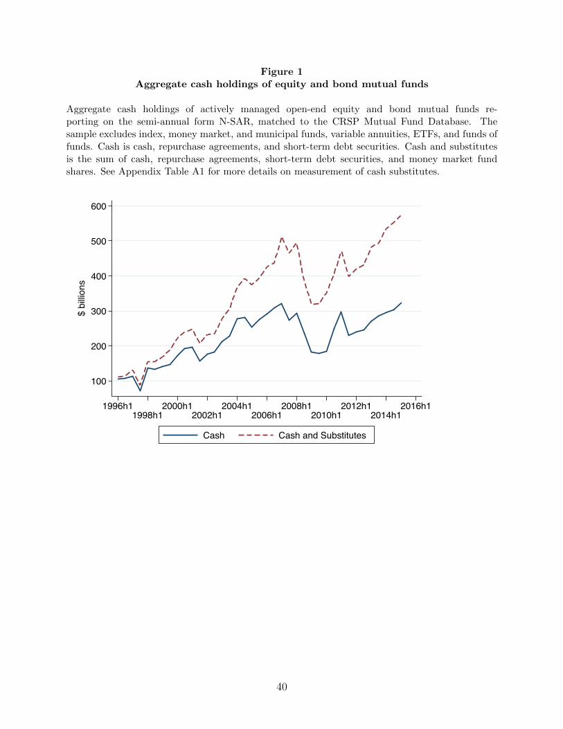
Figure 1Aggregate cash holdings of equity and bond mutual funds

Aggregate cash holdings of actively managed open-end equity and bond mutual funds re-porting on the semi-annual form N-SAR, matched to the CRSP Mutual Fund Database. Thesample excludes index, money market, and municipal funds, variable annuities, ETFs, and funds offunds. Cash is cash, repurchase agreements, and short-term debt securities. Cash and substitutesis the sum of cash, repurchase agreements, short-term debt securities, and money market fundshares. See Appendix Table A1 for more details on measurement of cash substitutes.

100

200

300

400

500

600

$ bi

llions

1996h11998h1

2000h12002h1

2004h12006h1

2008h12010h1

2012h12014h1

2016h1

Cash Cash and Substitutes

40

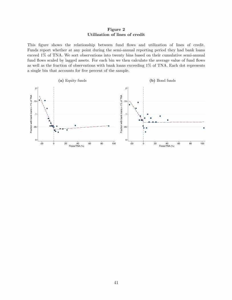
Figure 2Utilization of lines of credit

This figure shows the relationship between fund flows and utilization of lines of credit.Funds report whether at any point during the semi-annual reporting period they had bank loansexceed 1% of TNA. We sort observations into twenty bins based on their cumulative semi-annualfund flows scaled by lagged assets. For each bin we then calculate the average value of fund flowsas well as the fraction of observations with bank loans exceeding 1% of TNA. Each dot representsa single bin that accounts for five percent of the sample.

(a) Equity funds

0

.05

.1

.15

.2

Frac

tion

with

ban

k lo

ans

> 1%

of T

NA

-20 0 20 40 60 80 100Flows/TNA (%)

(b) Bond funds

0

.05

.1

.15

.2

Frac

tion

with

ban

k lo

ans

> 1%

of T

NA

-20 0 20 40 60 80 100Flows/TNA (%)

41

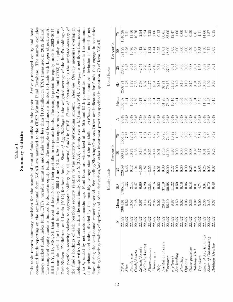
Tab

le1

Su

mm

ary

stati

stic

s

Th

ista

ble

rep

ort

ssu

mm

ary

stati

stic

sfo

rth

esa

mp

leof

mu

tual

fun

ds

stu

die

din

the

pap

er.

Act

ivel

ym

anag

edeq

uit

yan

db

ond

op

en-e

nd

fun

ds

rep

ort

ing

on

the

sem

i-an

nu

alfo

rmN

-SA

Rar

em

atch

edto

the

CR

SP

Mu

tual

Fu

nd

Dat

abas

e.T

he

sam

ple

excl

ud

esm

oney

mark

etfu

nd

s,in

dex

fun

ds,

ET

Fs,

vari

able

annu

itie

s,an

dfu

nd

sw

ith

less

than

$100

mil

lion

inT

NA

(mea

sure

din

2012

dol

lars

).T

he

sam

ple

of

equ

ity

fun

ds

isli

mit

edto

dom

esti

ceq

uit

yfu

nd

s.T

he

sam

ple

ofb

ond

fun

ds

isli

mit

edto

fun

ds

wit

hL

ipp

erob

ject

ives

A,

BB

B,

HY

,II

D,

MS

I,SII

that

inve

stat

least

50%

ofth

eir

por

tfol

ioin

corp

orat

eb

onds.

Th

esa

mp

lep

erio

dfo

req

uit

yfu

nd

sis

2003

–201

4.T

he

sam

ple

per

iod

for

bond

fun

ds

isJan

uar

y20

04–J

un

e20

12.Illiq

isth

esq

uar

e-ro

otve

rsio

nof

Am

ihu

d(2

002)

for

equ

ity

fun

ds

and

Dic

k-N

iels

en,

Fel

dh

utt

er,

and

Lan

do

(201

2)fo

rb

ond

fun

ds.

Share

ofAgg

Holdings

isth

ew

eigh

ted

-aver

age

ofth

efu

nd

’sh

old

ings

ofea

chp

ort

foli

ose

curi

tyre

lati

ve

toaggr

egate

hol

din

gsby

all

mu

tual

fun

ds

inC

RS

P.Share

ofOutstanding

isth

ew

eigh

ted

-ave

rage

ofth

efu

nd

’sh

old

ings

ofea

chp

ortf

oli

ose

curi

tyre

lati

veto

the

secu

rity

’sou

tsta

nd

ing

amou

nt.

Holdings

Overlap

mea

sure

sov

erla

pin

hold

ings

wit

hot

her

fun

ds

wit

hin

the

sam

efa

mil

y.Size

isln

(TNA

).Familysize

isln

(familyTNA

).Flows j→

kis

net

flow

sfr

omm

onth

jto

k,

scal

edby

net

asse

tssi

xm

onth

sago

.F

un

dfl

ows

are

win

sori

zed

atth

e5t

han

d95

thp

erce

nti

les.

Turnover

isth

em

inim

um

of

pu

rch

ases

and

sale

s,d

ivid

edby

the

mon

thly

aver

age

size

ofth

ep

ortf

olio

.σ

(Flows)

isth

est

and

ard

dev

iati

onof

mon

thly

net

flow

sd

uri

ng

the

sem

i-an

nu

alre

por

tin

gp

erio

d.

Sec

lend

ing/

Sh

orti

ng/

Op

tion

s/O

ther

are

ind

icat

ors

for

fun

ds

that

enga

gein

secu

riti

esle

nd

ing/

short

ing/

trad

ing

ofop

tion

san

doth

erd

eriv

ativ

es/a

nd

oth

erin

ves

tmen

tp

ract

ices

spec

ified

inqu

esti

on70

offo

rmN

-SA

R.

Equ

ity

fun

ds

Bon

dfu

nd

sP

erce

nti

leP

erce

nti

leN

Mea

nS

D25

50

75

NM

ean

SD

25

50

75

TNA

22,4

2720

64.8

15785.

14

228.5

9580.1

41554.8

72,6

48

1435.

07

2537.

71

233.7

6521.2

91346.2

8Size

22,4

276.

521.

33

5.4

36.3

67.3

52,6

48

6.41

1.23

5.4

56.2

67.2

1Familysize

22,4

2710.5

72.

14

9.1

210.7

412.0

12,6

48

10.

55

1.72

9.5

410.7

611.5

6Cash/Assets

22,4

277.

488.

47

1.9

44.3

69.5

22,6

48

7.89

7.53

2.5

55.2

810.7

6∆Cash/Assets

22,4

270.

676.

60

−1.

66

0.1

32.3

12,5

78

0.77

7.68

−2.

54

0.1

22.9

4∆

(Cash/Assets)

22,4

27−

0.14

5.20

−1.

87

−0.0

41.6

42,5

78

−0.

19

6.07

−2.

70

−0.

12

2.2

4Flows t−5→t−

322

,427

2.73

13.

84

−3.

55

−0.6

54.5

32,6

48

4.64

14.

75

−2.

38

1.3

27.2

5Flows t−2→t

22,4

272.

3612.

16

−3.

47

−0.4

44.7

62,6

48

4.61

14.

51

−2.

18

1.4

47.0

6Illiq

22,4

270.

020.

02

0.0

10.0

10.0

32,6

48

−0.

21

0.18

−0.

34

−0.

25

−0.

12

Institutionalshare

22,4

2729.1

937.

19

0.0

07.4

856.9

62,6

48

31.

28

37.

71

0.0

010.0

160.6

1Turnover

22,4

2756.1

050.

08

22.0

041.0

074.0

02,6

48

73.

48

79.

15

27.0

048.0

085.0

0σ

(Flows)

22,4

278.8

711.

22

2.2

74.9

310.7

22,6

48

10.

14

11.

76

3.0

16.0

512.4

7Sec

lending

22,4

270.

500.

50

0.0

00.0

01.0

02,6

48

0.41

0.49

0.0

00.0

01.0

0Shorting

22,4

270.

020.

16

0.0

00.0

00.0

02,6

48

0.04

0.19

0.0

00.0

00.0

0Options

22,4

270.

030.

06

0.0

00.0

00.0

02,6

48

0.05

0.10

0.0

00.0

00.1

2Other

practices

22,4

270.

360.

18

0.2

50.3

80.5

02,6

48

0.43

0.15

0.3

80.5

00.5

0Holdings

HHI

22,4

270.

020.

01

0.0

10.0

20.0

32,6

48

0.01

0.01

0.0

10.0

10.0

1Topshare

22,4

275.

004.

74

2.8

54.1

75.8

42,6

48

3.54

3.23

1.6

32.3

34.1

1Share

ofAgg

Holdings

22,4

272.

363.

84

0.2

50.8

12.6

92,6

48

11.

35

10.

88

3.8

77.5

014.6

6Share

ofOutstanding

22,4

270.

450.

72

0.0

50.1

60.5

02,6

48

1.45

1.92

0.3

40.7

21.5

7Holdings

Overlap

22,4

270.

370.

48

0.0

70.2

50.4

82,6

48

0.15

0.33

0.0

10.0

50.1

5

42

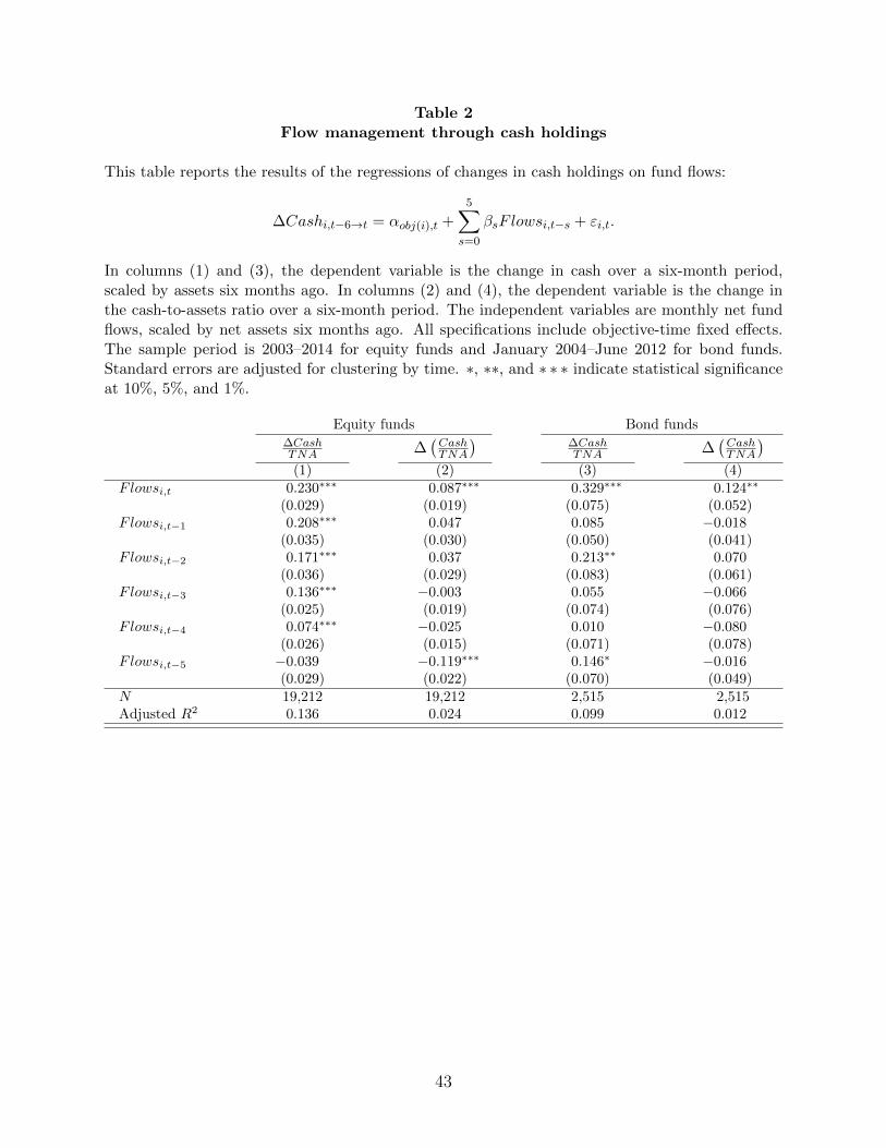
Table 2Flow management through cash holdings

This table reports the results of the regressions of changes in cash holdings on fund flows:

∆Cashi,t−6→t = αobj(i),t +5∑

s=0

βsFlowsi,t−s + εi,t.

In columns (1) and (3), the dependent variable is the change in cash over a six-month period,scaled by assets six months ago. In columns (2) and (4), the dependent variable is the change inthe cash-to-assets ratio over a six-month period. The independent variables are monthly net fundflows, scaled by net assets six months ago. All specifications include objective-time fixed effects.The sample period is 2003–2014 for equity funds and January 2004–June 2012 for bond funds.Standard errors are adjusted for clustering by time. ∗, ∗∗, and ∗ ∗ ∗ indicate statistical significanceat 10%, 5%, and 1%.

Equity funds Bond funds∆CashTNA ∆

(CashTNA

)∆CashTNA ∆

(CashTNA

)(1) (2) (3) (4)

Flowsi,t 0.230∗∗∗ 0.087∗∗∗ 0.329∗∗∗ 0.124∗∗

(0.029) (0.019) (0.075) (0.052)Flowsi,t−1 0.208∗∗∗ 0.047 0.085 −0.018

(0.035) (0.030) (0.050) (0.041)Flowsi,t−2 0.171∗∗∗ 0.037 0.213∗∗ 0.070

(0.036) (0.029) (0.083) (0.061)Flowsi,t−3 0.136∗∗∗ −0.003 0.055 −0.066

(0.025) (0.019) (0.074) (0.076)Flowsi,t−4 0.074∗∗∗ −0.025 0.010 −0.080

(0.026) (0.015) (0.071) (0.078)Flowsi,t−5 −0.039 −0.119∗∗∗ 0.146∗ −0.016

(0.029) (0.022) (0.070) (0.049)N 19,212 19,212 2,515 2,515Adjusted R2 0.136 0.024 0.099 0.012

43

Table 3Interactions with asset and market illiquidity

This table reports the result of the regressions of changes in cash holdings on fund flowsinteracted with (a) the fund’s asset illiquidity and (b) aggregate market illiquidity:

∆Cashi,t−6→t = αobj(i),t + β1Flowsi,t−2→t + β2Flowsi,t−2→t × Illiqi,t−6

+ β3Flowsi,t−5→t−3 + β4Flowsi,t−5→t−3 × Illiqi,t−6 + β5Illiqi,t−6 + εi,t.

In columns (1) and (3), the dependent variable is the change in cash over a six-month period,scaled by assets six months ago. In columns (2) and (4), the dependent variable is the changein the cash-to-assets ratio over a six-month period. Asset illiquidity is measured as of thebeginning of the six-month period and is standardized so that the coefficients on illiquidity and itsinteractions represent the effect of a one-standard deviation change in illiquidity. All specificationsinclude objective-time fixed effects. The sample period is 2003–2014 for equity funds and January2004–June 2012 for bond funds. Standard errors are adjusted for clustering by time. ∗, ∗∗, and∗ ∗ ∗ indicate statistical significance at 10%, 5%, and 1%.

Equity funds Bond funds∆CashTNA ∆

(CashTNA

)∆CashTNA ∆

(CashTNA

)(1) (2) (3) (4)

Panel A: Asset illiquidityFlowsi,t−2→t 0.171∗∗∗ 0.043∗∗∗ 0.146∗∗∗ 0.030

(0.010) (0.006) (0.030) (0.019)Flowsi,t−2→t × Illiqi,t−6 0.036∗∗∗ 0.016∗ 0.041∗ 0.015

(0.012) (0.009) (0.020) (0.016)Flowsi,t−5→t−3 0.082∗∗∗ −0.027∗∗∗ 0.143∗∗∗ −0.010

(0.013) (0.007) (0.035) (0.038)Flowsi,t−5→t−3 × Illiqi,t−6 0.016 −0.005 −0.041 −0.016

(0.010) (0.008) (0.037) (0.025)Illiqi,t−6 0.096 −0.063 0.398 0.157

(0.126) (0.079) (0.357) (0.306)N 19,212 19,212 2,515 2,515Adjusted R2 0.143 0.022 0.109 0.010

Panel B: Market illiquidityFlowsi,t−2→t 0.161∗∗∗ 0.037∗∗∗ 0.104∗∗ 0.011

(0.013) (0.007) (0.039) (0.022)Flowsi,t−2→t × Low Agg Liqt−2→t 0.049∗∗ 0.024∗ 0.123∗∗ 0.056

(0.022) (0.013) (0.058) (0.039)Flowsi,t−5→t−3 0.082∗∗∗ −0.029∗∗∗ 0.209∗∗∗ 0.056∗∗

(0.015) (0.006) (0.039) (0.025)Flowsi,t−5→t−3 × Low Agg Liqt−5→t−3 0.003 0.001 −0.183∗∗ −0.180∗∗

(0.027) (0.017) (0.066) (0.072)N 19,212 19,212 2,515 2,515Adjusted R2 0.139 0.022 0.113 0.021

44

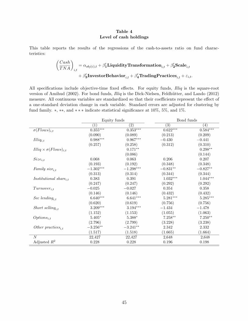
Table 4Level of cash holdings

This table reports the results of the regressions of the cash-to-assets ratio on fund charac-teristics: (

Cash

TNA

)i,t

= αobj(i),t + β′1LiquidityTransformationi,t + β′2Scalei,t

+ β′3InvestorBehaviori,t + β′4TradingPracticesi,t + εi,t.

All specifications include objective-time fixed effects. For equity funds, Illiq is the square-rootversion of Amihud (2002). For bond funds, Illiq is the Dick-Nielsen, Feldhutter, and Lando (2012)measure. All continuous variables are standardized so that their coefficients represent the effect ofa one-standard deviation change in each variable. Standard errors are adjusted for clustering byfund family. ∗, ∗∗, and ∗ ∗ ∗ indicate statistical significance at 10%, 5%, and 1%.

Equity funds Bond funds(1) (2) (3) (4)

σ(Flows)i,t 0.355∗∗∗ 0.353∗∗∗ 0.622∗∗∗ 0.584∗∗∗

(0.090) (0.089) (0.213) (0.209)Illiqi,t 0.988∗∗∗ 0.967∗∗∗ −0.430 −0.441

(0.257) (0.258) (0.312) (0.310)Illiq × σ(Flows)i,t 0.171∗∗ 0.298∗∗

(0.086) (0.144)Sizei,t 0.068 0.063 0.206 0.207

(0.193) (0.192) (0.348) (0.348)Family sizei,t −1.302∗∗∗ −1.298∗∗∗ −0.831∗∗ −0.827∗∗

(0.313) (0.314) (0.344) (0.344)Institutional sharei,t 0.383 0.391 1.032∗∗∗ 1.044∗∗∗

(0.247) (0.247) (0.292) (0.292)Turnoveri,t −0.025 −0.027 0.354 0.358

(0.146) (0.146) (0.432) (0.432)Sec lendingi,t 6.640∗∗∗ 6.641∗∗∗ 5.281∗∗∗ 5.285∗∗∗

(0.620) (0.619) (0.756) (0.756)Short sellingi,t 3.209∗∗∗ 3.194∗∗∗ −1.434 −1.478

(1.152) (1.153) (1.055) (1.063)Optionsi,t 5.405∗ 5.388∗ 7.258∗∗ 7.250∗∗

(2.796) (2.799) (3.228) (3.238)Other practicesi,t −3.256∗∗ −3.241∗∗ 2.342 2.332

(1.517) (1.518) (1.665) (1.664)N 22,427 22,427 2,648 2,648Adjusted R2 0.228 0.228 0.196 0.198

45

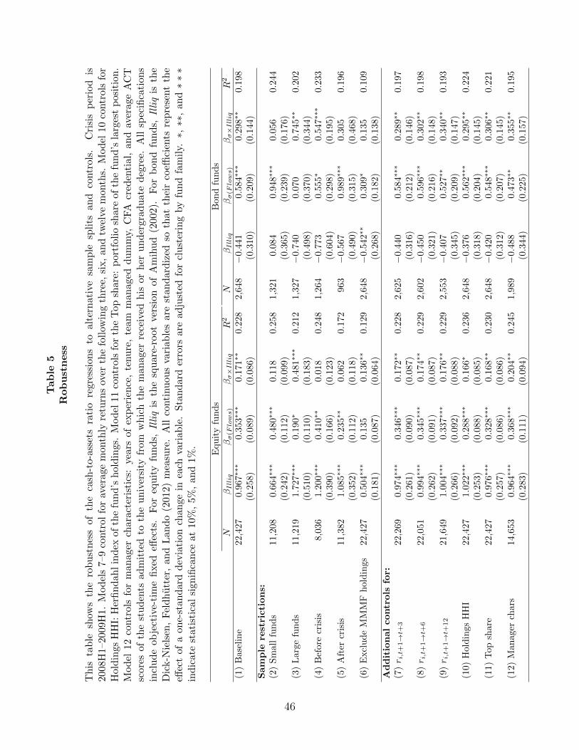
Tab

le5

Rob

ust

ness

Th

ista

ble

show

sth

ero

bu

stn

ess

ofth

eca

sh-t

o-as

sets

rati

ore

gres

sion

sto

alte

rnat

ive

sam

ple

spli

tsan

dco

ntr

ols.

Cri

sis

per

iod

is2008

H1–

2009

H1.

Mod

els

7–9

contr

olfo

rav

erag

em

onth

lyre

turn

sov

erth

efo

llow

ing

thre

e,si

x,

and

twel

vem

onth

s.M

od

el10

contr

ols

for

Hol

din

gs

HH

I:H

erfi

nd

ahl

ind

exof

the

fun

d’s

hol

din

gs.

Mod

el11

contr

ols

for

the

Top

shar

e:p

ortf

olio

shar

eof

the

fun

d’s

larg

est

pos

itio

n.

Mod

el12

contr

ols

for

man

ager

chara

cter

isti

cs:

year

sof

exp

erie

nce

,te

nu

re,

team

man

aged

du

mm

y,C

FA

cred

enti

al,

and

aver

age

AC

Tsc

ores

ofth

est

ud

ents

ad

mit

ted

toth

eu

niv

ersi

tyfr

omw

hic

hth

em

anag

erre

ceiv

edh

isor

her

un

der

grad

uat

ed

egre

e.A

llsp

ecifi

cati

ons

incl

ud

eob

ject

ive-

tim

efi

xed

effec

ts.

For

equ

ity

fun

ds,

Illiq

isth

esq

uar

e-ro

otver

sion

ofA

mih

ud

(200

2).

For

bon

dfu

nd

s,Illiq

isth

eD

ick-N

iels

en,

Fel

dh

utt

er,

and

Lan

do

(2012)

mea

sure

.A

llco

nti

nu

ous

vari

able

sar

est

and

ard

ized

soth

atth

eir

coeffi

cien

tsre

pre

sent

the

effec

tof

aon

e-st

an

dar

dd

evia

tion

chan

gein

each

vari

able

.S

tan

dar

der

rors

are

adju

sted

for

clu

ster

ing

by

fun

dfa

mil

y.∗,∗∗

,an

d∗∗∗

ind

icate

stat

isti

cal

sign

ifica

nce

at

10%

,5%

,an

d1%

.

Equ

ity

fun

ds

Bond

fun

ds

NβIlliq

βσ(Flows)

βσ×Illiq

R2

NβIlliq

βσ(Flows)

βσ×Illiq

R2

(1)

Bas

elin

e22

,427

0.96

7∗∗∗

0.353∗∗∗

0.171∗∗

0.2

28

2,6

48

−0.

441

0.5

84∗∗∗

0.2

98∗∗

0.1

98

(0.2

58)

(0.0

89)

(0.0

86)

(0.3

10)

(0.2

09)

(0.1

44)

Sam

ple

rest

ricti

on

s:(2

)S

mal

lfu

nd

s11

,208

0.6

64∗∗∗

0.480∗∗∗

0.118

0.2

58

1,3

21

0.084

0.9

48∗∗∗

0.0

56

0.2

44

(0.2

42)

(0.1

12)

(0.0

99)

(0.3

65)

(0.2

39)

(0.1

76)

(3)

Lar

gefu

nd

s11

,219

1.72

7∗∗∗

0.190∗

0.481∗∗∗

0.2

12

1,3

27

−0.

740

0.070

0.745∗∗

0.2

02

(0.5

10)

(0.1

10)

(0.1

83)

(0.4

98)

(0.3

70)

(0.3

44)

(4)

Bef

ore

cris

is8,

036

1.20

0∗∗∗

0.4

10∗∗

0.018

0.2

48

1,2

64

−0.

773

0.555∗

0.5

47∗∗∗

0.2

33

(0.3

90)

(0.1

66)

(0.1

23)

(0.6

04)

(0.2

98)

(0.1

95)

(5)

Aft

ercr

isis

11,3

821.

085∗∗∗

0.2

35∗∗

0.062

0.1

72

963

−0.

567

0.989∗∗∗

0.3

05

0.1

96

(0.3

52)

(0.1

12)

(0.1

18)

(0.4

90)

(0.3

15)

(0.4

68)

(6)

Excl

ud

eM

MM

Fh

old

ings

22,4

270.

504∗∗∗

0.1

35

0.136∗∗

0.1

29

2,6

48

−0.

542∗∗

0.309∗

0.1

35

0.1

09

(0.1

81)

(0.0

87)

(0.0

64)

(0.2

68)

(0.1

82)

(0.1

38)

Ad

dit

ion

al

contr

ols

for:

(7)r i,t+1→t+

322

,269

0.97

4∗∗∗

0.346∗∗∗

0.172∗∗

0.2

28

2,6

25

−0.

440

0.5

84∗∗∗

0.2

89∗∗

0.1

97

(0.2

61)

(0.0

90)

(0.0

87)

(0.3

16)

(0.2

12)

(0.1

46)

(8)r i,t+1→t+

622

,051

0.99

4∗∗∗

0.345∗∗∗

0.174∗∗

0.2

29

2,6

02

−0.

450

0.596∗∗∗

0.3

02∗∗

0.1

98

(0.2

62)

(0.0

91)

(0.0

87)

(0.3

21)

(0.2

16)

(0.1

48)

(9)r i,t+1→t+

12

21,6

491.

004∗∗∗

0.3

37∗∗∗

0.176∗∗

0.2

29

2,5

53

−0.

407

0.527∗∗

0.3

40∗∗

0.1

93

(0.2

66)

(0.0

92)

(0.0

88)

(0.3

45)

(0.2

09)

(0.1

47)

(10)

Hol

din

gsH

HI

22,4

271.0

22∗∗∗

0.2

88∗∗∗

0.166∗

0.2

36

2,6

48

−0.

376

0.562∗∗∗

0.2

95∗∗

0.2

24

(0.2

53)

(0.0

88)

(0.0

85)

(0.3

18)

(0.2

04)

(0.1

45)

(11)

Top

shar

e22

,427

0.97

6∗∗∗

0.3

28∗∗∗

0.168∗∗

0.2

30

2,6

48

−0.

420

0.548∗∗∗

0.3

06∗∗

0.2

21

(0.2

57)

(0.0

86)

(0.0

86)

(0.3

12)

(0.2

07)

(0.1

45)

(12)

Man

ager

char

s14

,653

0.9

64∗∗∗

0.3

68∗∗∗

0.204∗∗

0.2

45

1,9

89

−0.

488

0.473∗∗

0.3

55∗∗

0.1

95

(0.2

83)

(0.1

11)

(0.0

94)

(0.3

44)

(0.2

25)

(0.1

57)

46

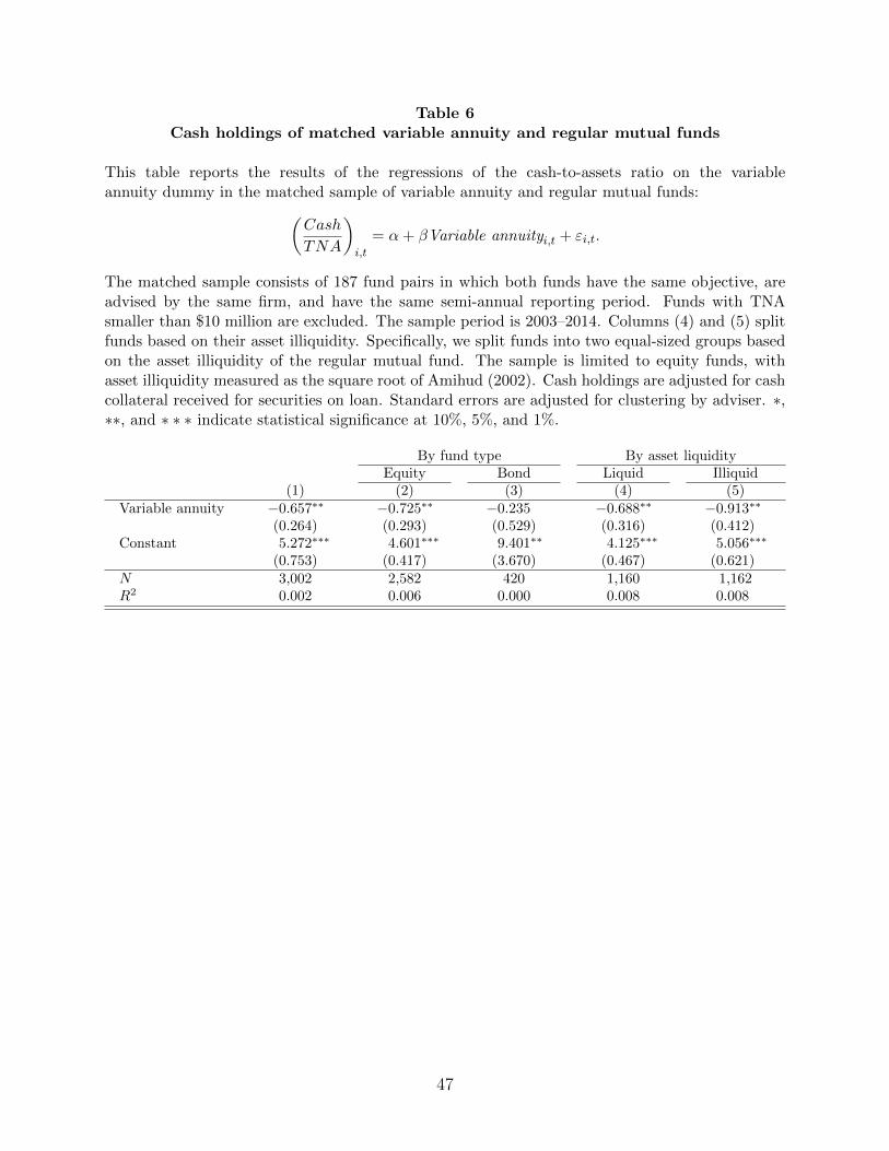
Table 6Cash holdings of matched variable annuity and regular mutual funds

This table reports the results of the regressions of the cash-to-assets ratio on the variableannuity dummy in the matched sample of variable annuity and regular mutual funds:(

Cash

TNA

)i,t

= α+ βVariable annuityi,t + εi,t.

The matched sample consists of 187 fund pairs in which both funds have the same objective, areadvised by the same firm, and have the same semi-annual reporting period. Funds with TNAsmaller than $10 million are excluded. The sample period is 2003–2014. Columns (4) and (5) splitfunds based on their asset illiquidity. Specifically, we split funds into two equal-sized groups basedon the asset illiquidity of the regular mutual fund. The sample is limited to equity funds, withasset illiquidity measured as the square root of Amihud (2002). Cash holdings are adjusted for cashcollateral received for securities on loan. Standard errors are adjusted for clustering by adviser. ∗,∗∗, and ∗ ∗ ∗ indicate statistical significance at 10%, 5%, and 1%.

By fund type By asset liquidityEquity Bond Liquid Illiquid

(1) (2) (3) (4) (5)Variable annuity −0.657∗∗ −0.725∗∗ −0.235 −0.688∗∗ −0.913∗∗

(0.264) (0.293) (0.529) (0.316) (0.412)Constant 5.272∗∗∗ 4.601∗∗∗ 9.401∗∗ 4.125∗∗∗ 5.056∗∗∗

(0.753) (0.417) (3.670) (0.467) (0.621)N 3,002 2,582 420 1,160 1,162R2 0.002 0.006 0.000 0.008 0.008

47

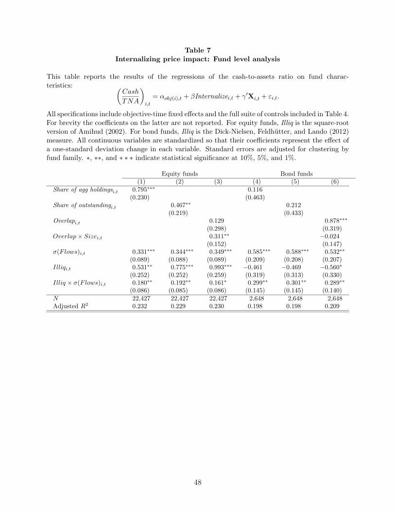
Table 7Internalizing price impact: Fund level analysis

This table reports the results of the regressions of the cash-to-assets ratio on fund charac-teristics: (

Cash

TNA

)i,t

= αobj(i),t + βInternalizei,t + γ′Xi,t + εi,t.

All specifications include objective-time fixed effects and the full suite of controls included in Table 4.For brevity the coefficients on the latter are not reported. For equity funds, Illiq is the square-rootversion of Amihud (2002). For bond funds, Illiq is the Dick-Nielsen, Feldhutter, and Lando (2012)measure. All continuous variables are standardized so that their coefficients represent the effect ofa one-standard deviation change in each variable. Standard errors are adjusted for clustering byfund family. ∗, ∗∗, and ∗ ∗ ∗ indicate statistical significance at 10%, 5%, and 1%.

Equity funds Bond funds(1) (2) (3) (4) (5) (6)

Share of agg holdingsi,t 0.795∗∗∗ 0.116(0.230) (0.463)

Share of outstandingi,t 0.467∗∗ 0.212(0.219) (0.433)

Overlapi,t 0.129 0.878∗∗∗

(0.298) (0.319)Overlap× Sizei,t 0.311∗∗ −0.024

(0.152) (0.147)σ(Flows)i,t 0.331∗∗∗ 0.344∗∗∗ 0.349∗∗∗ 0.585∗∗∗ 0.588∗∗∗ 0.532∗∗

(0.089) (0.088) (0.089) (0.209) (0.208) (0.207)Illiqi,t 0.531∗∗ 0.775∗∗∗ 0.993∗∗∗ −0.461 −0.469 −0.560∗

(0.252) (0.252) (0.259) (0.319) (0.313) (0.330)Illiq × σ(Flows)i,t 0.180∗∗ 0.192∗∗ 0.161∗ 0.299∗∗ 0.301∗∗ 0.289∗∗

(0.086) (0.085) (0.086) (0.145) (0.145) (0.140)N 22,427 22,427 22,427 2,648 2,648 2,648Adjusted R2 0.232 0.229 0.230 0.198 0.198 0.209

48

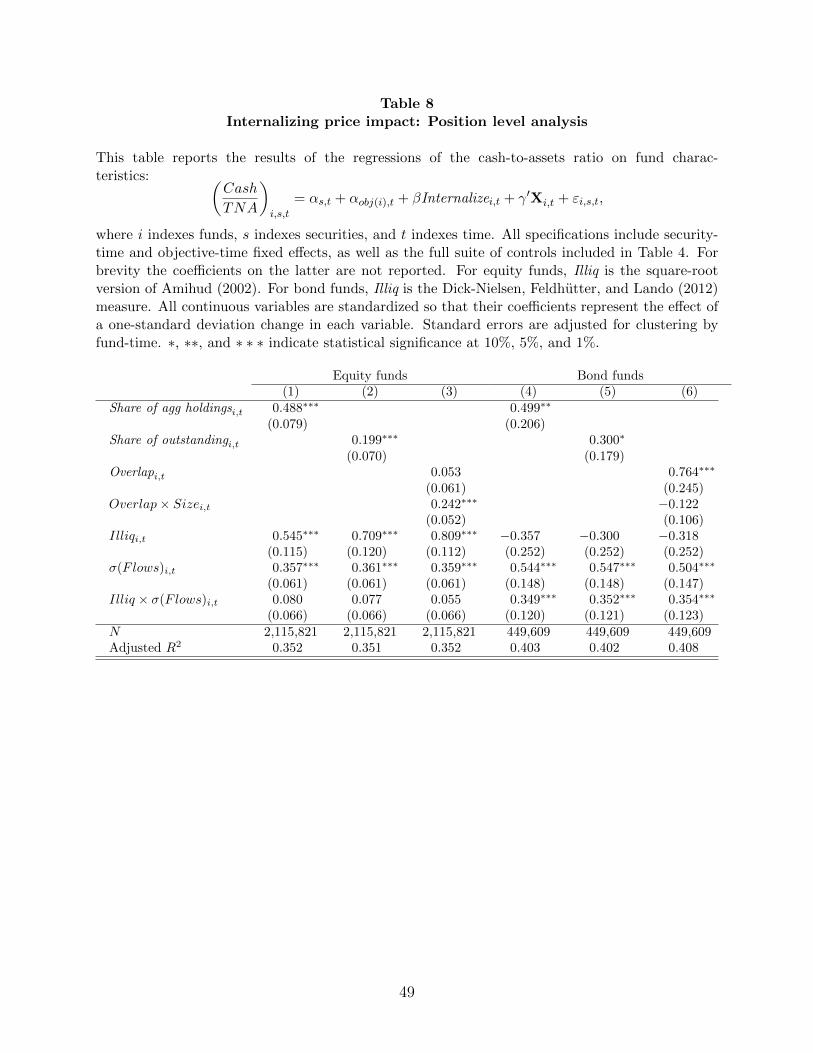
Table 8Internalizing price impact: Position level analysis

This table reports the results of the regressions of the cash-to-assets ratio on fund charac-teristics: (

Cash

TNA

)i,s,t

= αs,t + αobj(i),t + βInternalizei,t + γ′Xi,t + εi,s,t,

where i indexes funds, s indexes securities, and t indexes time. All specifications include security-time and objective-time fixed effects, as well as the full suite of controls included in Table 4. Forbrevity the coefficients on the latter are not reported. For equity funds, Illiq is the square-rootversion of Amihud (2002). For bond funds, Illiq is the Dick-Nielsen, Feldhutter, and Lando (2012)measure. All continuous variables are standardized so that their coefficients represent the effect ofa one-standard deviation change in each variable. Standard errors are adjusted for clustering byfund-time. ∗, ∗∗, and ∗ ∗ ∗ indicate statistical significance at 10%, 5%, and 1%.

Equity funds Bond funds(1) (2) (3) (4) (5) (6)

Share of agg holdingsi,t 0.488∗∗∗ 0.499∗∗

(0.079) (0.206)Share of outstandingi,t 0.199∗∗∗ 0.300∗

(0.070) (0.179)Overlapi,t 0.053 0.764∗∗∗

(0.061) (0.245)Overlap× Sizei,t 0.242∗∗∗ −0.122

(0.052) (0.106)Illiqi,t 0.545∗∗∗ 0.709∗∗∗ 0.809∗∗∗ −0.357 −0.300 −0.318

(0.115) (0.120) (0.112) (0.252) (0.252) (0.252)σ(Flows)i,t 0.357∗∗∗ 0.361∗∗∗ 0.359∗∗∗ 0.544∗∗∗ 0.547∗∗∗ 0.504∗∗∗

(0.061) (0.061) (0.061) (0.148) (0.148) (0.147)Illiq × σ(Flows)i,t 0.080 0.077 0.055 0.349∗∗∗ 0.352∗∗∗ 0.354∗∗∗

(0.066) (0.066) (0.066) (0.120) (0.121) (0.123)N 2,115,821 2,115,821 2,115,821 449,609 449,609 449,609Adjusted R2 0.352 0.351 0.352 0.403 0.402 0.408

49

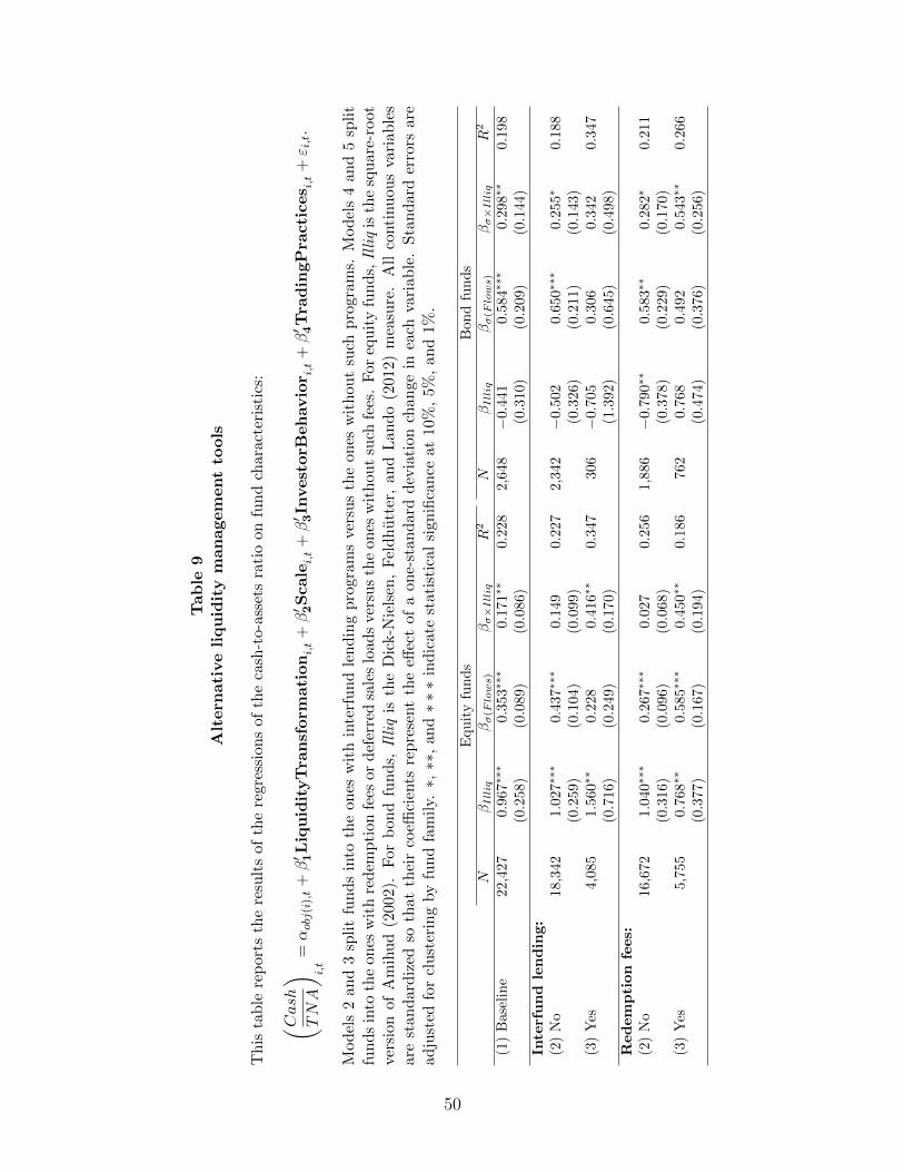
Tab

le9

Alt

ern

ati

ve

liqu

idit

ym

an

agem

ent

tools

Th

ista

ble

rep

ort

sth

ere

sult

sof

the

regr

essi

ons

ofth

eca

sh-t

o-as

sets

rati

oon

fun

dch

arac

teri

stic

s:

( Cash

TNA

) i,t

=αobj

(i),t+β′ 1L

iqu

idit

yT

ran

sform

ati

oni,t+β′ 2S

cale

i,t+β′ 3In

vest

orB

eh

avio

r i,t

+β′ 4T

rad

ingP

racti

ces i,t

+ε i,t.

Mod

els

2an

d3

spli

tfu

nd

sin

toth

eon

esw

ith

inte

rfu

nd

len

din

gp

rogr

ams

vers

us

the

ones

wit

hou

tsu

chp

rogr

ams.

Mod

els

4an

d5

spli

tfu

nd

sin

toth

eon

esw

ith

red

emp

tion

fees

or

def

erre

dsa

les

load

sve

rsu

sth

eon

esw

ith

out

such

fees

.F

oreq

uit

yfu

nd

s,Illiq

isth

esq

uar

e-ro

otve

rsio

nof

Am

ihu

d(2

002

).F

orb

on

dfu

nd

s,Illiq

isth

eD

ick-N

iels

en,

Fel

dh

utt

er,

and

Lan

do

(201

2)m

easu

re.

All

conti

nu

ous

vari

able

sar

est

an

dard

ized

soth

atth

eir

coeffi

cien

tsre

pre

sent

the

effec

tof

aon

e-st

and

ard

dev

iati

onch

ange

inea

chva

riab

le.

Sta

nd

ard

erro

rsar

ead

just

edfo

rcl

ust

erin

gby

fun

dfa

mil

y.∗,∗∗

,an

d∗∗∗

ind

icat

est

atis

tica

lsi

gnifi

can

ceat

10%

,5%

,an

d1%

.

Equ

ity

fun

ds

Bon

dfu

nd

sN

βIlliq

βσ(Flows)

βσ×Illiq

R2

NβIlliq

βσ(Flows)

βσ×Illiq

R2

(1)

Bas

elin

e22

,427

0.9

67∗∗∗

0.353∗∗∗

0.1

71∗∗

0.2

28

2,6

48

−0.

441

0.5

84∗∗∗

0.2

98∗∗

0.1

98

(0.2

58)

(0.0

89)

(0.0

86)

(0.3

10)

(0.2

09)

(0.1

44)

Inte

rfu

nd

len

din

g:

(2)

No

18,3

421.0

27∗∗∗

0.437∗∗∗

0.1

49

0.2

27

2,3

42

−0.

502

0.6

50∗∗∗

0.2

55∗

0.1

88

(0.2

59)

(0.1

04)

(0.0

99)

(0.3

26)

(0.2

11)

(0.1

43)

(3)

Yes

4,08

51.5

60∗∗

0.2

28

0.4

16∗∗

0.3

47

306

−0.7

05

0.3

06

0.3

42

0.3

47

(0.7

16)

(0.2

49)

(0.1

70)

(1.3

92)

(0.6

45)

(0.4

98)

Red

em

pti

on

fees:

(2)

No

16,6

721.0

40∗∗∗

0.267∗∗∗

0.0

27

0.2

56

1,8

86

−0.

790∗∗

0.5

83∗∗

0.2

82∗

0.2

11

(0.3

16)

(0.0

96)

(0.0

68)

(0.3

78)

(0.2

29)

(0.1

70)

(3)

Yes

5,75

50.7

68∗∗

0.5

85∗∗∗

0.4

50∗∗

0.1

86

762

0.7

68

0.4

92

0.5

43∗∗

0.2

66

(0.3

77)

(0.1

67)

(0.1

94)

(0.4

74)

(0.3

76)

(0.2

56)

50

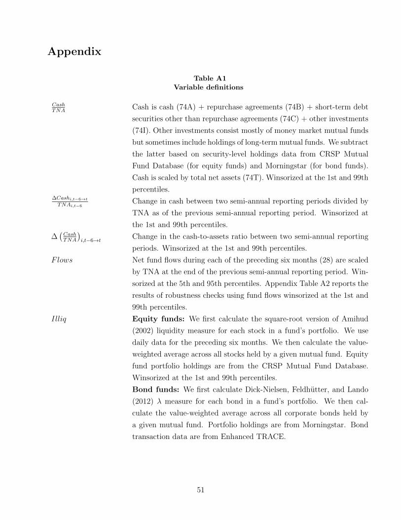
Appendix

Table A1Variable definitions

CashTNA

Cash is cash (74A) + repurchase agreements (74B) + short-term debt

securities other than repurchase agreements (74C) + other investments

(74I). Other investments consist mostly of money market mutual funds

but sometimes include holdings of long-term mutual funds. We subtract

the latter based on security-level holdings data from CRSP Mutual

Fund Database (for equity funds) and Morningstar (for bond funds).

Cash is scaled by total net assets (74T). Winsorized at the 1st and 99th

percentiles.∆Cashi,t−6→t

TNAi,t−6Change in cash between two semi-annual reporting periods divided by

TNA as of the previous semi-annual reporting period. Winsorized at

the 1st and 99th percentiles.

∆(CashTNA

)i,t−6→t

Change in the cash-to-assets ratio between two semi-annual reporting

periods. Winsorized at the 1st and 99th percentiles.

Flows Net fund flows during each of the preceding six months (28) are scaled

by TNA at the end of the previous semi-annual reporting period. Win-

sorized at the 5th and 95th percentiles. Appendix Table A2 reports the

results of robustness checks using fund flows winsorized at the 1st and

99th percentiles.

Illiq Equity funds: We first calculate the square-root version of Amihud

(2002) liquidity measure for each stock in a fund’s portfolio. We use

daily data for the preceding six months. We then calculate the value-

weighted average across all stocks held by a given mutual fund. Equity

fund portfolio holdings are from the CRSP Mutual Fund Database.

Winsorized at the 1st and 99th percentiles.

Bond funds: We first calculate Dick-Nielsen, Feldhutter, and Lando

(2012) λ measure for each bond in a fund’s portfolio. We then cal-

culate the value-weighted average across all corporate bonds held by

a given mutual fund. Portfolio holdings are from Morningstar. Bond

transaction data are from Enhanced TRACE.

51

Table A1—Continued

Low Agg Liq For equity funds, we use the Pastor and Stambaugh (2003) measure

of market liquidity. For bond funds, we use the aggregate version of

Dick-Nielsen, Feldhutter, and Lando (2012). Periods of low aggregate

liquidity are defined as those in the bottom tercile of the distribution

of aggregate market liquidity within our sample.

Family size Log of aggregate TNA across all CRSP mutual funds within the same

family.

σ(Flows) Standard deviation of monthly fund flows (28) over the preceding six

months. Fund flows are scaled by TNA as of the beginning of the

semi-annual reporting period.

Institutional share Fraction of institutional share classes, identified following Chen, Gold-

stein, and Jiang (2010). A share class is considered to be institutional

if a) CRSPs institutional dummy is equal to Y and retail dummy is

equal to N, or b) fund name includes the word institutional or its ab-

breviation, or c) class name includes one of the following suffixes: I, X,

Y, or Z. Share classes with the word retirement in their name or J, K,

and R suffixes are considered to be retail.

Turnover Portfolio turnover for the current semi-annual reporting period (71D).

Portfolio turnover is the minimum of purchases and sales (including

all maturities), divided by the monthly average value of the portfolio.

Portfolio turnover is winsorized at the 1st and 99th percentiles.

Sec lending Binary variable equal to one for funds that engage in loaning portfolio

securities (70N).

Short selling Binary variable equal to one for funds that engage in short selling (70R).

Options Average of 8 binary variables, each equal to one if a fund engages

in writing or investing in 1) options on equities (70B), 2) options on

debt securities (70C), 3) options on stock indices (70D), 4) interest

rate futures (70E), 5) stock index futures (70F), 6) options on futures

(70G), 7) options on stock index futures (70H), and 8) other commodity

futures (70I).

52

Table A1—Continued

Other practices Average of 7 binary variables for engaging in the following investment

practices: 1) investment in restricted securities (70J), 2) investment in

shares of other investment companies (70K), 3) investment in securi-

ties of foreign issuers (70L), 4) currency exchange transactions (70M),

5) borrowing of money (70O), 6) purchases/sales by certain exempted

affiliated persons (70P), 7) margin purchases (70Q).

Redemption fees Binary variable equal to one for funds that impose a deferred or contin-

gent deferred sales load (34) or a redemption fee other than a deferred

or contingent sales load (37).

Share of agg holdings Weighted-average of the fund’s holdings of each security relative to

aggregate holdings by all mutual funds:∑

sVf,s∑s Vf,s

× Vf,s∑f Vf,s

, where f

indexes funds and s indexes securities. For equities (bonds), aggregate

fund holdings are calculated using CSRP (Morningstar).

Share of outstanding Weighted-average of the fund’s holdings of each portfolio security rel-

ative to the security’s outstanding amount:∑

sVf,s∑s Vf,s

× Vf,s

Outstandings,

where f indexes funds and s indexes securities. For stocks, the out-

standing is the market capitalization, calculated using the price and

number of shares reported in CRSP. For bonds, outstanding is the face

value at issuance.

Overlap For each security s held by fund f , we calculate aggregate holdings of

security s by all other funds that belong to the same family and divide

this by the aggregate TNA of family funds, excluding fund f . We then

calculate the value-weighted average across all securities held by fund

f . Specifically, Overlapf =∑

sVf,s∑s Vf,s

×∑

j∈family(f),j 6=f Vf,s∑j∈family(f),j 6=f TNAj

, where f

and j index funds and s indexes securities.

Tenure Number of years managing the fund. For team managed funds, Tenure

is the average across individual managers. Manager identities and char-

acteristics are from Morningstar and cover the period through Septem-

ber 2013.

Experience Number of years managing any mutual funds.

ACT Average ACT score of the students admitted to the university from

which the fund manager received his or her undergraduate degree. ACT

scores are for the 2001–2002 incoming class. Source: National Center

for Education Statistics, IPEDS Data Center.

53

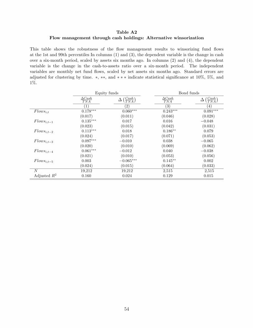
Table A2Flow management through cash holdings: Alternative winsorization

This table shows the robustness of the flow management results to winsorizing fund flowsat the 1st and 99th percentiles In columns (1) and (3), the dependent variable is the change in cashover a six-month period, scaled by assets six months ago. In columns (2) and (4), the dependentvariable is the change in the cash-to-assets ratio over a six-month period. The independentvariables are monthly net fund flows, scaled by net assets six months ago. Standard errors areadjusted for clustering by time. ∗, ∗∗, and ∗ ∗ ∗ indicate statistical significance at 10%, 5%, and1%.

Equity funds Bond funds∆CashTNA ∆

(CashTNA

)∆CashTNA ∆

(CashTNA

)(1) (2) (3) (4)

Flowsi,t 0.178∗∗∗ 0.060∗∗∗ 0.243∗∗∗ 0.091∗∗∗

(0.017) (0.011) (0.046) (0.028)Flowsi,t−1 0.135∗∗∗ 0.017 0.016 −0.048

(0.023) (0.015) (0.042) (0.031)Flowsi,t−2 0.113∗∗∗ 0.018 0.186∗∗ 0.079

(0.024) (0.017) (0.071) (0.053)Flowsi,t−3 0.097∗∗∗ −0.010 0.038 −0.065

(0.020) (0.010) (0.069) (0.062)Flowsi,t−4 0.061∗∗∗ −0.012 0.040 −0.038

(0.021) (0.010) (0.053) (0.056)Flowsi,t−5 0.003 −0.065∗∗∗ 0.145∗∗ 0.002

(0.024) (0.015) (0.064) (0.033)N 19,212 19,212 2,515 2,515Adjusted R2 0.160 0.024 0.129 0.015

54

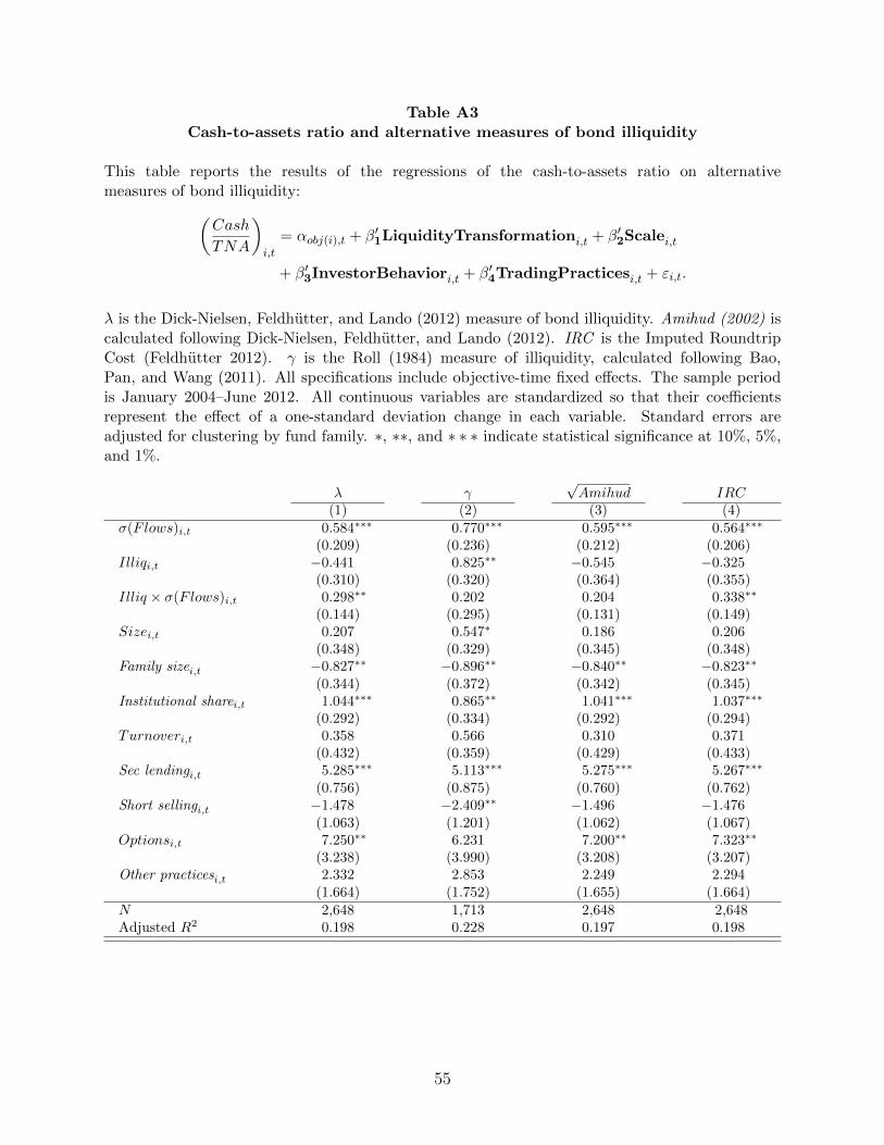
Table A3Cash-to-assets ratio and alternative measures of bond illiquidity

This table reports the results of the regressions of the cash-to-assets ratio on alternativemeasures of bond illiquidity:(

Cash

TNA

)i,t

= αobj(i),t + β′1LiquidityTransformationi,t + β′2Scalei,t

+ β′3InvestorBehaviori,t + β′4TradingPracticesi,t + εi,t.

λ is the Dick-Nielsen, Feldhutter, and Lando (2012) measure of bond illiquidity. Amihud (2002) iscalculated following Dick-Nielsen, Feldhutter, and Lando (2012). IRC is the Imputed RoundtripCost (Feldhutter 2012). γ is the Roll (1984) measure of illiquidity, calculated following Bao,Pan, and Wang (2011). All specifications include objective-time fixed effects. The sample periodis January 2004–June 2012. All continuous variables are standardized so that their coefficientsrepresent the effect of a one-standard deviation change in each variable. Standard errors areadjusted for clustering by fund family. ∗, ∗∗, and ∗ ∗ ∗ indicate statistical significance at 10%, 5%,and 1%.

λ γ√Amihud IRC

(1) (2) (3) (4)σ(Flows)i,t 0.584∗∗∗ 0.770∗∗∗ 0.595∗∗∗ 0.564∗∗∗

(0.209) (0.236) (0.212) (0.206)Illiqi,t −0.441 0.825∗∗ −0.545 −0.325

(0.310) (0.320) (0.364) (0.355)Illiq × σ(Flows)i,t 0.298∗∗ 0.202 0.204 0.338∗∗

(0.144) (0.295) (0.131) (0.149)Sizei,t 0.207 0.547∗ 0.186 0.206

(0.348) (0.329) (0.345) (0.348)Family sizei,t −0.827∗∗ −0.896∗∗ −0.840∗∗ −0.823∗∗

(0.344) (0.372) (0.342) (0.345)Institutional sharei,t 1.044∗∗∗ 0.865∗∗ 1.041∗∗∗ 1.037∗∗∗

(0.292) (0.334) (0.292) (0.294)Turnoveri,t 0.358 0.566 0.310 0.371

(0.432) (0.359) (0.429) (0.433)Sec lendingi,t 5.285∗∗∗ 5.113∗∗∗ 5.275∗∗∗ 5.267∗∗∗

(0.756) (0.875) (0.760) (0.762)Short sellingi,t −1.478 −2.409∗∗ −1.496 −1.476

(1.063) (1.201) (1.062) (1.067)Optionsi,t 7.250∗∗ 6.231 7.200∗∗ 7.323∗∗

(3.238) (3.990) (3.208) (3.207)Other practicesi,t 2.332 2.853 2.249 2.294

(1.664) (1.752) (1.655) (1.664)N 2,648 1,713 2,648 2,648Adjusted R2 0.198 0.228 0.197 0.198

55

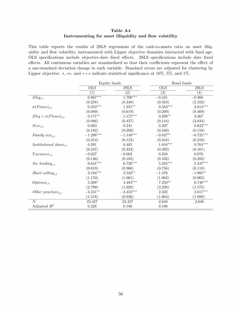
Table A4Instrumenting for asset illiquidity and flow volatility

This table reports the results of 2SLS regressions of the cash-to-assets ratio on asset illiq-uidity and flow volatility, instrumented with Lipper objective dummies interacted with fund age.OLS specifications include objective-date fixed effects. 2SLS specifications include date fixedeffects. All continuous variables are standardized so that their coefficients represent the effect ofa one-standard deviation change in each variable. Standard errors are adjusted for clustering byLipper objective. ∗, ∗∗, and ∗ ∗ ∗ indicate statistical significance at 10%, 5%, and 1%.

Equity funds Bond fundsOLS 2SLS OLS 2SLS(1) (2) (3) (4)

Illiqi,t 0.967∗∗∗ 1.700∗∗∗ −0.441 −0.368(0.258) (0.348) (0.310) (2.102)

σ(Flows)i,t 0.353∗∗∗ 1.231∗∗ 0.584∗∗∗ 2.614∗∗∗

(0.089) (0.619) (0.209) (0.469)Illiq × σ(Flows)i,t 0.171∗∗ 1.175∗∗∗ 0.298∗∗ 3.267

(0.086) (0.437) (0.144) (3.834)Sizei,t 0.063 0.241 0.207 0.622∗∗∗

(0.192) (0.200) (0.348) (0.158)Family sizei,t −1.298∗∗∗ −1.148∗∗∗ −0.827∗∗ −0.725∗∗∗

(0.314) (0.123) (0.344) (0.216)Institutional sharei,t 0.391 0.405 1.044∗∗∗ 0.764∗∗∗

(0.247) (0.324) (0.292) (0.161)Turnoveri,t −0.027 −0.002 0.358 0.070

(0.146) (0.105) (0.432) (0.282)Sec lendingi,t 6.641∗∗∗ 6.726∗∗∗ 5.285∗∗∗ 5.347∗∗∗

(0.619) (0.966) (0.756) (0.118)Short sellingi,t 3.194∗∗∗ 2.532∗∗ −1.478 −1.985∗∗

(1.153) (1.061) (1.063) (0.965)Optionsi,t 5.388∗ 4.484∗∗∗ 7.250∗∗ 6.748∗∗∗

(2.799) (1.020) (3.238) (1.575)Other practicesi,t −3.241∗∗ −3.452∗∗∗ 2.332 3.017∗∗∗

(1.518) (0.836) (1.664) (1.088)N 22,427 22,427 2,648 2,648Adjusted R2 0.228 0.186 0.198 .

56