Liquidity-Saving Mechanisms in Collateral-Based RTGSPayment Systems

Marius JurgilasBank of England

Antoine Martin∗

Federal Reserve Bank of New York

September 1, 2009

Abstract

This paper studies banks’ incentives regarding the timing of payment submissionsin a collateral-based RTGS payment system and how these incentives change with theintroduction of a liquidity-saving mechanism (LSM). We show that an LSM allowsbanks to economize on collateral while also providing incentives to submit paymentsearlier. This is because an LSM allows payments to be matched and offset, helping toeliminate payment cycles where each banks needs to receive a payment in order to haveenough funds to send its payment. In contrast to fee-based systems, for which Martinand McAndrews (2008a) show that introducing an LSM can lead to higher welfare, weshow that welfare is always higher with an LSM in a collateral-based system.

JEL CLASSIFICATION: E42, E58, G21KEY WORDS: Liquidity Saving Mechanism, intra-day liquidity, payments

∗The views expressed herein are those of the authors and do not necessarily reflect the views of the Bankof England, the Federal Reserve Bank of New York, or the Federal Reserve System

1

1 Introduction

A growing recognition of the key role played by payments systems in modern economies

has lead to increasing interest in the behavior of such systems. Research on payment

system has also been motivated by the important design changes that have occurred in

the last thirty years from delayed net settlement system to real-time gross settlement

(RTGS) system and, more recently, with the introduction of liquidity saving mecha-

nisms in many countries. This research has shown that the incentives embedded in

a payment system are sensitive to its design, highlighting the importance of a better

understanding of these incentives.1

There are two main types of RTGS payment systems that differ in the way banks

can obtain access to intraday reserves from the central bank. In a collateral-based

system, such as TARGET 2 (European Central Bank), CHAPS (Bank of England),

or SIC (Swiss National Bank), banks can obtain intraday reserves at no fee against

collateral. In contrast, in a fee-based system such as Fewire (Federal Reserve) banks

can obtain intraday reserves without collateral but at a fee.2

This paper studies the effect of introducing a liquidity-saving mechanism (LSM) in

a collateral-based RTGS system. Our model is closely related to the model proposed

by Martin and McAndrews (2008a), which studies fee-base settlement systems. The

similarity allows us to compare and contrast our results. We show that, absent an

LSM, banks face a trade-off between the cost of collateral and the cost of delay. By

increasing their initial collateral, banks face lower expected cost of delays. Introducing

an LSM allows banks to reduce their need for collateral while providing incentives for

payments to be submitted early. A reduced need for collateral is beneficial because

tying up collateral in the payment system can be costly for bank, as this collateral may

have better use in other markets. Early submission of payments is also beneficial as it

reduces the risk associated with operational failures if payment are concentrated late

in the day.

We also study the planner’s allocation for our economy. Without an LSM, the

equilibrium allocation may be different from the planner’s allocation as the planner

takes into account the effect of a bank’s actions on other banks. For some parameter

values, however, the equilibrium and the planner’s allocation are the same. When they

1See Martin and McAndrews (2008b) for example.2Note that the Federal Reserve has adopted a new policy that will allow banks to choose be-

tween collateralized overdrafts at no fee or uncollateralized overdrafts for a fee. For more details, seehttp://www.federalreserve.gov/paymentsystems/psr/default.htm.

1

are not, there is too much delay in equilibrium. In contrast, the equilibrium and the

planner’s allocation are the same for all parameter values with an LSM.

The incentives of banks are different in fee-based compared to collateral-based sys-

tem. In a fee-based system, banks choose whether to submit or delay a payment by

comparing the cost of borrowing from the central bank with the cost of delaying the

payment. The marginal cost of borrowing is a fixed fee per unit of reserve borrowed,

so the terms of the trade-off will depend on the amount each bank expects to bor-

row. In a collateral-based system, banks choose their initial level of collateral at the

beginning of the day, before they must make decisions about whether to submit or

delay payments. A bank that is below its collateral limit will face no marginal cost of

sending a payment. Because increasing collateral during the day is costly, banks are

likely to prefer to delay payments rather than obtain more collateral, if the collateral

limit binds. Hence, we can think of banks as belonging to two groups: Banks that have

sufficient collateral for their payment to settle regardless of incoming payments face no

cost of submitting payments. Banks that have insufficient collateral risk hitting their

collateral constraint if they submit a payment.

This difference in incentives between the two systems results in differences in out-

come. A notable feature of fee-based RTGS systems is that they exhibit multiple

equilibria. The intuition is that if many banks send their payments early, the probabil-

ity of receiving a payment early is high so that the expected cost of borrowing is low.

A low expected cost of borrowing gives incentives for banks to send their payments

early. A similar argument applies in reverse to the case where few banks send their

payments early. Multiple equilibria can occur in collateral-based RTGS systems as

well, but are less important. In particular, the multiplicity disappears if all payments

form bilaterally offsetting pairs. The intuition is as follows: If a bank has sufficient

liquidity, then it will submit its payment early regardless of what its counterparty does.

If the bank has insufficient liquidity, then its payment can settle only if it receives a

payment from its counterparty. This can happen only if the counterparty has sufficient

collateral. Hence, there is no strategic interactions between banks that may have an

incentive to delay; namely those with insufficient liquidity. Strategic interactions reap-

pear when some payments are not bilaterally offsetting. Nevertheless, the number of

possible equilibria is higher in a fee-based system that in a collateral-based system.

In a collateral-based system, the equilibrium allocation without an LSM can be the

same as the planner’s allocation, for some parameter values. This is in contrast to the

2

results in Atalay, Martin, and McAndrews (2008), which show that there is always too

much delay in equilibrium, so that the planner’s allocation cannot be achieved.

In fee-based RTGS systems, Martin and McAndrews (2008a) show that introducing

an LSM can lead to a decrease in welfare, for some parameter values. In contrast, an

LSM always leads to higher welfare in our model of a collateral-based system. Indeed,

we show that with an LSM, the equilibrium and the planner’s allocation are always

the same. Introducing an LSM increases welfare in a collateral-based system in two

ways: it allows offsetting of payments and allows banks to economize on their collateral.

Offsetting of payments prevents situations where a group of banks form a cycle and

each bank needs to receive a payment from its counterparty to have enough reserve

for its own payment to settle. Atalay et al. (2008) show that for some, but not all,

parameter values, the equilibrium allocation with an LSM can be the same as the

planner’s allocation.

The remainder of the paper is structured as follows. In Section 2 we review the

literature. In Section 3 we develop a benchmark theoretical model for collateralized

RTGS payment system and characterize the equilibria. We introduce an LSM in Section

4 and compare the payment system with and without an LSM. In section 5, we study

the planner’s allocation with and without an LSM, and contrast the results with the

equilibrium allocations. Section 6 concludes.

2 Literature review

The incentive structure of the RTGS payment systems is well analyzed in the literature.

Angelini (1998, 2000) and Bech and Garratt (2003) provide theoretical argumentation

as to why banks may find it optimal to delay payments in RTGS system. This, appears

to be not only a theoretical possibility, but a practical feature of some of the payment

systems. Armantier, Arnold, and McAndrews (2008) show that a large proportion of

payments in Fedwire are settled late in the day with the peak around 17:11 in 2006.

Significant intra-day payment delays carry a non-pecuniary cost of “delay” (ie customer

satisfaction), but most importantly it can exacerbate the costs of an operational failure

or costs due to the default of a payment system participant.

This paper is closely related to Martin and McAndrews (2008a) and Atalay et al.

(2008). The two papers analyze the effects of introducing LSMs in a real-time gross

settlement system with a fee based intra-day credit. Martin and McAndrews (2008a)

classify possible equilibria that could result from introducing LSMs. They show that

3

apart from netting, queuing arrangements allow banks to condition their payments

on the receipt of the offsetting payments. Thus via LSM arrangements banks can

contract on the individual intra-day liquidity shocks. Such a possibility is not present

in a system without netting.

The benefits of LSM are also analyzed by Roberds (1999), Kahn and Roberds

(2001) and Willison (2005). We extend these studies on different dimensions. Most

importantly we consider the effect of liquidity shocks on payment behavior.

3 Model

The economy lasts for two periods, morning and afternoon. There are infinitely many

identical agents, called banks, and a non-optimizing agent, called settlement systems.

Banks make payments to each other and to the settlement systems.

Bank may receive three types of payment orders: A bank may be required to transfer

funds to the settlement systems. We refer to such payments as “liquidity shocks” as

they cannot be delayed and must be executed immediately. Such payments represent

contractual obligation to be settled immediately and any delay constitutes a default.

Example of such payments are margin calls in securities settlement systems or foreign

exchange settlement. A bank may also be required to transfer funds to another bank. In

this case we distinguish between urgent payments, having the property that the bank

suffers a delay cost, γ, if the payment is not executed immediately, and non-urgent

payments, which can be delayed without any cost.

By the end of the day, each bank must send, and will receive, one payment of size

µ ∈ [1/2, 1] from another bank. At the beginning of the morning period, each bank

learns if it must send a payment to, or receive a payment from, the settlement systems.

These payments determine the bank’s liquidity shock, denoted by λ. If a bank must

send a payment, λ = −1, if it receives a payment, λ = 1, otherwise λ = 0. We assume

that the probability of λ = 1 is equal to the probability of λ = −1, and is denoted by

π ∈ [0, 0.5]. The probability of λ = 0 is 1− 2π. The size of payments to and from the

settlements systems is 1− µ.

At the beginning of the morning period, banks also learn whether the payment they

must send to another bank is urgent, which occurs with probability θ, or non-urgent,

which occurs with probability 1 − θ. Banks know the urgency of the payment they

must send, but not the payment they receive. For example, if a payment is made on

behalf of a customer, the sending bank will know how quickly the customer wants the

4

payment to be send but the receiving bank may not even be aware of the fact that a

payment is forthcoming for one of its customers.

The combination of the urgency of the payment a bank must make to another bank

and its liquidity shock determine a bank’s type. Hence, banks can be of six types: A

bank may have to send an urgent or a non-urgent payment and may receive a negative, a

positive, or no liquidity shock. We assume that a bank’s liquidity shock is uncorrelated

with the urgency of the payment it must make to another bank. Banks do not know

the type of their counterparties, but only the distribution of types in the population.

Also, since the number of banks is large, there are no strategic interactions. While this

is a limitation for some payments system, such as the UK, where the actual number

of banks is small, anecdotal evidence suggests that banks do not make their liquidity

management strategies contingent on the strategies of the other banks. Instead, banks

appear to make their payment flow decisions contingent on the realized payment flows

from their counterparties.

Banks must hold enough reserves on their central bank account for the payments

they send to settle. If necessary, banks can borrow reserves from the central bank

at a net interest rate of zero, against collateral. We assume, however, that posting

collateral is costly. Banks choose an initial collateral level, at a cost κ per unit, before

learning their type. κ corresponds to the opportunity cost of the collateral as well as

the cost of bringing collateral from the securities settlement system to the payments

system. At the end of the morning period, payments are delayed if available collateral

is insufficient. Payments must be settled by the end of the day, however, so delay is

not an option at the end of the afternoon period. Additional collateral can be obtained

at any time during the day at a cost of Ψ > κ.

In modeling the need for collateral, we abstract from two considerations: (i) Banks

may also post collateral to satisfy prudential liquidity requirement, which we ignore,

and (ii) banks usually start the day with a positive settlement account balance to

satisfy reserve requirements, for example. We assume that initial settlement balances

are zero for all banks in the model and focus only on the incentive to hold collateral

due to payment flows. Hence, the reserves available for a bank’s payment to settle are

given by the collateral posted to the central bank and incoming payments only.

The timing of events during the day is as follows:

• Beginning of morning period:

– Banks choose the level of collateral L0 to be posted at the central bank (cost

5

κ per unit)

– Banks learn their type. If L0 insufficient to absorb the liquidity shock, addi-

tional collateral must be posted (cost Ψ per unit)3

– banks decide to send their payment to other banks or delay them until the

afternoon

• End of morning period:

– Incoming morning payments are observed

– If available collateral is insufficient payments are delayed unless additional

collateral is posted (cost Ψ per unit)

• Afternoon period:

– All unpaid payment orders executed. If collateral is insufficient, addition

collateral must be posted (cost Ψ per unit)

We make two parameter restrictions concerning the cost of adding collateral during

the day, Ψ. First, we assume that πΨ ≥ κ, so banks choose a level of initial collateral

of at least 1 − µ, so they have enough collateral to settle a negative liquidity shock.

Second, we assume (1−µ)Ψ ≥ max{R, π(R+γ)}, which guarantees that banks always

prefer to delay a payment at the end of the morning period, rather than pay that

cost.4 It is not possible to avoid that cost at the end of the afternoon period, since all

payments must be settled before the end of the day.

Banks that receive a negative liquidity shock need to obtain reserves so their reserve

account is non-negative at the end of the day. We assume that an overnight money

market in which banks can obtain such reserves opens at the end of the day. Since this

represents a fixed cost, it does not influence the intraday behavior of banks and we

ignore it in the remainder of the paper. In other words, we assume that the intraday

and overnight reserve management of banks are independent.

To facilitate the comparison with fee-based systems, our model is closely related

to the model developed in Martin and McAndrews (2008a). In both models there are

6 types of banks, as banks can receive a positive, a negative, or no liquidity shock,

and banks may have to send a time-critical payment. In Martin and McAndrews

(2008a) banks that need to borrow at the CB face a fee. In contrast, borrowing from

the CB is free in our model, provided the bank has enough collateral. Despite the

3We assume that liquidity shocks cannot be settled using the funds that a bank accumulates due toincoming payments

4Available data suggests that banks very rarely increase their collateral during the day.

6

similarities between the model, our results differ from Martin and McAndrews (2008a)

in interesting ways.

3.1 A bank’s problem

The problem of a bank consists of choosing an initial level of collateral, L0, as well as

whether to send or delay its payment to another bank, to minimize its expected cost.

In this section, we provide the notation and derive the expressions needed to solve that

problem. In particular, we derive expressions for the expected cost of a bank in the

morning period and in the afternoon period.

Let P = 1 if a bank sends its payment in the morning period. Note that sending a

payment in the morning does not guarantee that the payment will settle during that

period. Similarly, P = 0 if the bank delays its payment until the afternoon. The

amount of collateral available to a bank after it observes its liquidity shock but before

it chooses whether so send or delay its payment to another bank, L1, is the sum of the

initial collateral posted by the bank and its liquidity shock. It is given by

L1 = max{L0 + λ(1− µ), 0}.

If the bank does not have sufficient collateral to meet the liquidity shock, that is

L0 + λ(1− µ) < 0, it must obtain additional collateral.

We use φ as an indicator variable for a bank’s payment activity with other banks.

If a bank sends a payment to another bank in the morning, the payment settles, and

the bank does not receive an offsetting payment, then φ = −1. If the bank does not

send a payment to, but receives a payment from, another bank in the morning, then

φ = 1. If a payment sent to another bank settles in the same period as the payment

received from another bank, then φ = 0.

We can derive expressions for the probability of each of these events. These prob-

abilities depend on whether a bank sends a payment in the morning and, if the bank

sends a payment, whether it settles. The probability that a payment settles in the

morning depends on the amount of collateral the bank has. Let πs denote the prob-

ability of receiving a payment conditional on sending a payment and having enough

collateral for the payment to settle, even if a payment from a another bank is not

received. The superscript ‘s’ indicates that the bank has ‘sufficient’ collateral. We use

πi to denote the probability of receiving a payment conditional on sending a payment

that can settle only if a payment is received. The superscript ‘i’ indicates that the

7

bank has ‘insufficient’ collateral. Note that the probability of receiving a payment if

the bank delays is also equal to πi. Banks form rational expectations about πi and πs,

which are determined in equilibrium.

A bank has φ = −1 if it submits a payment, P = 1, and has enough collateral for

the payment to settle, I(L1 ≥ µ), despite the fact that it does not receive a payment

from another bank, 1− πs:

Prob(φ = −1) = PI(L1 ≥ µ)(1− πs). (3.1)

A bank has φ = 0 either if it does not send a payment and does not receive one, or if it

sends a payment that does not settle, or if it sends a payment that settles and receives

a payment. This last case occurs with a different probability depending on whether

the bank has sufficient collateral. We can write

Prob(φ = 0) = (1− P )(1− πi) + PI(L1 < µ) + PI(L1 ≥ µ)πs. (3.2)

The first term indicates that the bank does not send a payment and does not receive

one. The second term corresponds to the case where a bank submits a payment without

sufficient collateral. Regardless of the incoming payments the net balance will be zero

(either no payment is received and the outgoing payment cannot be settled, or an

incoming payment is received and the outgoing payment is settled). The third term

corresponds to a bank with sufficient collateral that sends and receives a payment.

Finally, a bank has φ = 1 if it receives, but does not send, a payment:

Prob(φ = 1) = (1− P )πi. (3.3)

Now can write the expression for the cost faced by a bank at the end of the morning

period. If a bank sends a payment that fails to settle, it incurs a reputational or

resubmission cost of R > 0. The cost function for the morning period for a bank with

an urgent payment is:

C1 = κL0 −Ψmin{L0 + λ(1− µ), 0}+

+PI(L1 < µ)(1− πi)(R + γ) + (1− P )γ. (3.4)

The bank pays a cost κ per unit for its initial choice of collateral. In addition, it must

pay Ψ per unit of collateral if L0 + λ(1−µ) < 0, so that its payment to the settlement

systems can be sent. Recall that we assume that a bank prefers to delay a payment

to another bank rather than increase its collateral level at cost Ψ. If 0 ≤ L1 < µ, a

8

payment sent does not settle if the bank does not receive an offsetting payment, which

occurs with probability (1− πi). In such a case the bank faces a resubmission cost R,

and a delay cost γ. If the bank does not send a payment, it faces a delay cost. The

expression for a bank with a non-urgent payment is similar, but γ is replaced by zero,

since there is no delay cost.

The amount of collateral available to the bank in the afternoon is denoted L2:

L2 = L1 + φµ.

Note, that L2 ≥ 0 as φ = −1 only if L1 ≥ µ.

We have assumed that payments sent and received to other banks offset. Never-

theless, payments may not settle without additional collateral in some cases. Consider

a bank that is part of a chain of banks, indexed by n ∈ {1, 2, ..., N}, forming a cycle.

Bank 1 sends a payment to bank 2, bank 2 sends a payment to bank 3, ..., and bank

N sends a payment to bank 1. If at least one of these banks has sufficient collateral, so

that its payment can settle even if it does not receive an offsetting payment, then this

payment triggers the settlement of all other payments in the cycle. If, instead, none

of the banks have sufficient collateral, then all payments are stuck. In such a case, we

assume that one of the banks must obtain additional collateral at cost Ψ per unit. The

probability that a given bank in the cycle needs to add collateral is 1/N . We denote

the expected cost of having to add collateral at the end of the day with Γ. Note, that

if the payment sent by a bank settles in the morning, then the bank will face no cost

in the afternoon. A bank risks being stuck in a payment cycle, exposing it to the need

to add collateral, only if the bank’s payment needs to settle in the afternoon. Hence,

the cost function for the afternoon period is given by:

C2 = [(1− P )(1− πi) + PI(L1 < µ)(1− πi)]max{µ− L1, 0}Γ. (3.5)

The first term in the square brackets corresponds to the case where a bank did not

send and did not receive a payment in the morning. The second term corresponds to

the case where the bank did send a payment in the morning, but the payment did not

settle because the bank did not have enough collateral and did not receive an offsetting

payment. We can write a bank’s problem as follows:

minL0

Eλ,γ

[min

PEφ

(C1 + C2)]

.

9

3.2 Banks’ behavior

The decision to pay or to delay a payment depends on λ and γ, as banks make a

decision after observing the realization of liquidity shock and the type of payments to

be made.

Proposition 1. All banks submit payments early if L1 ≥ µ

Proof. If after receiving a liquidity shock a bank has enough liquidity to make a pay-

ment it will do so. The expected cost of making a payment, ECP , is:

ECP = L0κ

while the cost of delaying a payment, ECD, is:

ECD = L0κ + γ.

Therefore, unless γ ≤ 0 a bank is strictly better off by making a payment early. As

shown in Table 1 L1 ≥ µ in region R1, region R2 if no negative liquidity shock was

received, and region R3 if a positive liquidity shock was received.

Proposition 2. Banks with L1 < µ and a time-critical payment delay if (1− πi)(R +

γ) > γ

Proof. In this case after receiving a liquidity shock a bank does not have sufficient

liquidity to make a payment. If a bank submits early, with probability 1−πi there will

be no early incoming payment and a bank will experience a cost of R + γ. If a bank

chooses to delay, a payment is delayed with certainty and be a delay cost of γ realized.

ECP = L0κ + [...] + (R + γ)(1− πi)

ECD = L0κ + [...] + γ

The term in the brackets represents the cost of obtaining additional collateral during

the day and depends on the choice of L0. For our purposes it suffices to know that it

does not change regardless of the decision to pay early or to delay.

Proposition 3. If L1 < µ banks with a non-time critical payment delay.

Proof. Banks with γ = 0 would find it optimal to delay if R ≤ πiR. This is true if

and only if πi = 1. But as shown in Lemma 6 (Section 3.2) it cannot be the case in

equilibrium.

10

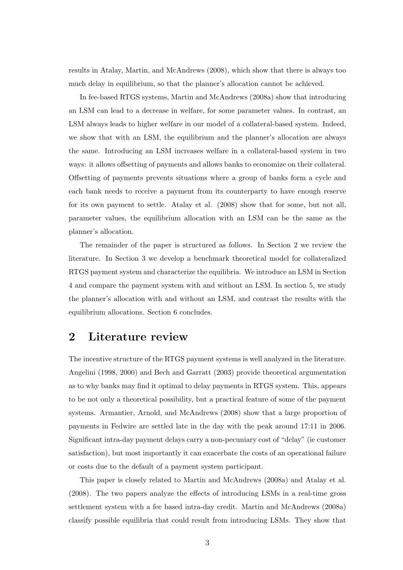
Table 1 summarizes under what conditions a bank will delay a payment, for various

values of its initial collateral, L0, and its liquidity shock, λ. The notation R1, ..., R6

indicates the region corresponding to each case in Figure 1.

Figure 1: Combinations of L0 (y axis) and µ (x axis) corresponding to different regions ofTable 1

Table 1: Optimal P given λ, L0, and γ.L0 region λ Delay if

-1 γ < 0 (never)L0 ≥ 1 0 γ < 0 (never)[R1] 1 γ < 0 (never)

-1 (1− πi)(R + γ) > γµ ≤ L0 < 1 0 γ < 0 (never)

[R2] 1 γ < 0 (never)2µ− 1 ≤ L0 < µ -1 (1− πi)(R + γ) > γand 1− µ ≤ L0 0 (1− πi)(R + γ) > γ

[R3] 1 γ < 0 (never)-1 (1− πi)(R + γ) > γ

1− µ ≤ L0 < 2µ− 1 0 (1− πi)(R + γ) > γ[R4] 1 (1− πi)(R + γ) > γ

-1 (1− πi)(R + γ) > γ0 ≤ L0 < 1− µ 0 (1− πi)(R + γ) > γ

[R5] 1 (1− πi)(R + γ) > γ-1 (1− πi)(R + γ) > γ

2µ− 1 ≤ L0 < 1− µ 0 (1− πi)(R + γ) > γ[R6] 1 γ < 0 (never)

11

3.3 Equilibrium

Given banks’ behavior described in Table 1 we can derive the equilibrium probability

of receiving a payment in the morning and the expected cost associated with a given

choice of initial collateral. We study symmetric Nash equilibria in pure strategies. We

focus on the case where µ ≥ 1/2, so the size of liquidity shocks, 1 − µ, is relatively

small. This is empirically plausible and simplifies the analysis.

In the morning, after banks observe their liquidity shock, we can distinguish three

groups: Some banks may delay their payment until the afternoon; we denote the share

of these banks τd. Some banks submit their payment and have enough collateral for

their payment to settle even if they do not receive an offsetting payment we denote

the share of these banks τs. Finally, some banks submit their payment but do not

have enough collateral for their payment to settle if they do not receive an offsetting

payment; we denote the share of these banks τi. Note that τd + τs + τi = 1. Abusing

terminology, we say that a bank is of type τj if it is part of the group of bank of size

τj , j = d, s, i.

The payments that banks make to each other form cycles, an example of which was

provided above. For simplicity, we assume that all such cycles have the same lengths. In

particular, we will focus on two cases: cycles of length two, in which case the payments

of a pair of banks are bilaterally offsetting, and the case where all payments form a

unique cycle.

In equilibrium, the probability πs depends on the length of the payment cycle. If

n = 2, πs = 1 − τd = τs + τi. In that case, it is enough that the bank’s counterparty

sends a payment, regardless of the amount of collateral the counterparty has. For

n = 3, πs = τs + τi(1 − τd) = τs + τi(τi + τs). The first term corresponds to the case

where bank 1 receives a payment from bank 2 and bank 2 has sufficient collateral. The

second term corresponds to the case where bank 1 receives a payment from bank 2

and bank 2 has insufficient collateral. However, bank 3 sends a payment and may or

may not have sufficient collateral. This is enough since, by assumption, bank 1 sends

a payment to bank 3. Extending the same argument for a cycle of length n, we obtain:

πs = τn−1i +

n−2∑k=0

τsτki . (3.6)

If τi < 1 and n →∞, then

πs =τs

τs + τd. (3.7)

12

Similarly, in equilibrium πi = τs if n = 2, since a bank with ‘insufficient’ collateral

can only receive a payment if its counterparty sends a payment and has ‘sufficient’

collateral. If n = 3, then πi = τs + τsτi. In that case, either the bank’s counterparty

has sufficient collateral, or the counterparty has insufficient collateral but receives a

payment from a bank with sufficient collateral. For any n,

πi =n−2∑k=0

τsτki . (3.8)

If τi < 1 and n →∞:

πi =τs

τs + τd. (3.9)

We can also derive an equilibrium value for Γ. First we need to find the probability

that none of the other banks have made a payment. Given the payment cycle length

of n this happens with the probability of (1− τs)n−1. Therefore

Γ =(1− τs)n−1

nΨ < Ψ. (3.10)

Proposition 4. Banks delay non-urgent payments (γ = 0) if, after receiving a liquidity

shock, they do not have sufficient collateral.

Proof. From Table 1 banks with insufficient collateral delay payments if (1− πi)(R +

γ) > γ. Thus, we have 3 possible cases:

1. (1− πi)(R + γ) > γ which also means that R > πiR

2. (1− πi)(R + γ) ≤ γ and R > πiR

3. (1− πi)(R + γ) ≤ γ and R ≤ πiR

Case 3 implies that πi = 1 and according to Lemma 6 (in Section 3.2) cannot be an

equilibrium. Therefore the only viable cases are Case 1 and 2. In both cases banks

with γ = 0 choose to delay their payments.

Based on Table 1 and on equations (3.4) and (3.5), we can write the expected

cost faced by banks for different values of L0 and on the relative values of γ and

(1−πi)(R+γ). Consider, for example, the case where µ ≤ L0 < 1 and (1−πi)(R+γ) ≤

γ. In this case, banks with a positive or no liquidity shock have sufficient collateral

and, as indicated by Table 1, send their payment in the morning. These banks face

no cost, other than the cost of the initial collateral. Banks with a negative liquidity

shock delay non-time critical payments. In such a case, the bank faces no cost in

the morning. Banks with a negative liquidity shock send time-critical payments in the

13

morning. With probability 1−πi, the payment does not settle and the bank face a cost

R + γ. These banks will face no cost in the afternoon if they receive a payment in the

morning. If they don’t, they may have to add an amount µ−L1 = 1−L0 of collateral

in the afternoon, at a cost Γ. Hence, the expected afternoon cost is (1− πi)(1−L0)Γ.

Using similar reasoning, we obtain the following expected costs: if (1−πi)(R+γ) > γ,

then

ECR2 = L0κ + γθπ + Γ(1− πi)(1− L0)π,

ECR3 = L0κ + γθ(1− π) + Γ(1− πi)(µ− (2µ− 1)π − L0(1− π)),

ECR4 = L0κ + γθ + Γ(1− π)(µ− L0),

and if (1− πi)(R + γ) ≤ γ, then

ECR2 = L0κ + (1− πi)(R + γ)θπ + Γ(1− πi)(1− L0)π,

ECR3 = L0κ + (1− πi)(R + γ)θ(1− π) + Γ(1− πi)(µ− (2µ− 1)π − L0(1− π)),

ECR4 = L0κ + (1− πi)(R + γ)θ + Γ(1− π)(µ− L0).

As noted earlier, we assume that the cost of obtaining collateral during the day, Ψ, is

large compared to the initial cost of positing collateral, κ, so that banks always choose

L0 ≥ 1− µ. This eliminates regions R5 and R6.

The next two lemmas show that only a few values of the banks’ choice of initial

capital are consistent with an equilibrium.

Lemma 5. Any value for of L0 different from L0 ∈ {1−µ, 2µ−1, µ, 1} cannot support

an equilibrium

Proof. Inspection of equations (3.4) and (3.5) show that L0 affects the expected cost

of banks directly and through πi. The value of πi depends on the faction of banks such

that L0 < µ + λ(1 − µ), for λ ∈ −1, 0, 1. Hence, the value of πi can only change at

the thresholds values L0 ∈ {2µ− 1, µ, 1}. For a given value of πi, equations (3.4) and

(3.5) show that costs decrease with respect to L0. We have assumed that banks never

choose L0 < 1− µ as the cost Ψ is too high compared to κ. Hence, banks will choose

L0 ∈ {1− µ, 2µ− 1, µ, 1}

Lemma 6. In equilibrium, πi < 1 and L0 < 1.

Proof. Suppose, instead, that πi = 1. This can only be true if all banks choose L0 = 1,

since banks with a negative liquidity shock do not have ‘sufficient’ collateral if L0 < 1.

14

However, L0 = 1 cannot be an equilibrium since a deviating bank would face πi = 1

and find it optimal to choose a smaller level of collateral.

It follows from the last two lemmas that we can restrict our attention to L0 ∈

{1− µ, 2µ− 1, µ}.

3.4 A long payment cycle

Assuming a unique payment cycle, the equilibrium probabilities of receiving a payment

in the morning are:

πi = πs =τs

1− τi. (3.11)

Notice that πi depends on τi, so there are strategic interactions between banks with

‘insufficient’ collateral. These strategic interactions are responsible for the presence of

multiple equilibria.

We derive the expected costs under different assumptions about the parameter

values. First we choose a value for L0 and, based on Table 1, we derive the value of τd,

τi, and τs depending on the relative value of γ and (1− πi)(R + γ). This allows us to

find the value of πi, which we can then use to write the expected cost faced by banks.

If L0 = µ and (1− πi)(R + γ) ≤ γ, then based on Table 1

• τd = π(1− θ),

• τi = πθ,

• τs = 1− π.

Using these values for τi and τs, we find

πi =1− π

1− πθ≥ 1− π. (3.12)

Hence, if L0 = µ and (1− 1−π1−πθ )(R + γ) ≤ γ, the expected cost is

EC

(L0 = µ, (1− 1− π

1− πθ)(R + γ) ≤ γ

)= µκ + (R + γ)θ(1− θ)

π2

1− θπ. (3.13)

If, instead, (1− πi)(R + γ) > γ, then

• τd = π,

• τi = 0,

• τs = 1− π = πi.

15

Notice that the value of πi in this case is different from what it was above. Hence, if

L0 = µ and π(R + γ) > γ, the expected cost is

EC (L0 = µ, π(R + γ) > γ) = µκ + γθπ. (3.14)

If

1− π ≤ R

R + γ≤ 1− π

1− πθ,

there are multiple equilibria. Intuitively, if banks with ‘insufficient’ collateral submit

their payments in the morning, rather than delay them, then the probability πi of

receiving a payment is high: πi = 1−π1−πθ and (1 − 1−π

1−πθ )(R + γ) ≤ γ. This provides

incentives for such banks to submit their payments early. In contrast, if banks with

‘insufficient’ collateral delay their payments, then the probability πi of receiving a

payment is low: πi = 1− π and π(R + γ) > γ. This provides incentives for such banks

to delay their payments.

We use similar steps in the other cases. If L0 = 2µ − 1 and (1 − πi)(R + γ) ≤ γ,

then

• τd = (1− π)(1− θ),

• τi = (1− π)θ,

• τs = π.

Hence,

πi =π

1− (1− π)θ≥ π (3.15)

and

EC

(L0 = 2µ− 1, (1− π

1− (1− π)θ)(R + γ) ≤ γ

)= (2µ− 1)κ + (R + γ)

(1− π)2(1− θ)θ1− (1− π)θ

. (3.16)

If, instead, (1− πi)(R + γ) > γ, then

• τd = (1− π),

• τi = 0,

• τs = π = πi,

and

EC (L0 = 2µ− 1, (1− π)(R + γ) > γ) = (2µ− 1)κ + γθ(1− π). (3.17)

16

There are multiple equilibria if

π ≤ R

R + γ≤ π

1− (1− π)θ.

Finally, if L0 = 1− µ, then πi = 0. So, the only relevant case is R + γ > γ and the

expected cost is

EC(L0 = 1− µ,R > 0) = (1− µ)κ + γθ. (3.18)

The expected costs described in equations (3.13), (3.14), (3.16), (3.17), and (3.18)

each consist of two terms: the first term expresses the cost of initial collateral, the

second term is the expected cost of delay and, potentially, the reputational cost R.

Holding more collateral allows banks to reduce their expected delay and reputational

cost.

For a given set of parameters, we can determine the equilibrium level of initial col-

lateral, L0 ∈ {1−µ, 2µ−1, µ}, by comparing the relevant expected costs. Determining

the equilibrium in each region of the parameter space is straightforward but tedious.

Instead, we consider some illustrative examples to provide some intuition.

Consider the region where

(1− 1− π

1− θπ)(R + γ) > γ. (3.19)

In this region, we need to compare equations (3.14), (3.17), and (3.18). Let W (L0 = x)

denote the welfare associated with L0 = x. We find that

W (L0 = µ) > W (L0 = 2µ− 1) ⇔ (1− 2π)θγ > (1− µ)κ, (3.20)

W (L0 = 2µ− 1) > W (L0 = 1− µ) ⇔ πθγ > (3µ− 2)κ, (3.21)

W (L0 = µ) > W (L0 = 1− µ) ⇔ (1− π)θγ > (2µ− 1)κ. (3.22)

These equations show that a higher value of κ, makes a high value of L0 less desirable.

In contrast, a higher value of θγ, the product of the probability of having a time-critical

payment and the cost of delay, makes a high value of L0 more desirable.

The effect of the probability of liquidity shocks, π, is more complicated. Consider

the effect of π: a higher value of π makes it more likely that a lower value of L0 will be

preferred to L0 = µ. However, it also makes it more likely that L0 = 2µ−1 is preferred

to L0 = 1−µ. To get some intuition, notice that if π → 1/2, the probability of having

zero shock vanishes, and banks are almost certain to experience either a positive or a

negative liquidity shock. When comparing L0 = µ with L0 = 2µ− 1 the bank realizes

that probability close to a half, it has ‘sufficient’ collateral, and probability close to a

17

half, it has ‘insufficient’ collateral. Hence, the cost of delay is almost the same for both

cases. Hence, the primary consideration becomes the cost of initial collateral, and the

bank will prefer a low level of collateral.

The reasoning is similar when comparing L0 = µ and L0 = 1−µ. With L0 = 1−µ,

the bank does not have sufficient collateral even when it receives a positive shock. As π

increases, the probability that a bank with L0 = µ has ‘insufficient’ collateral increases.

So the advantage of having high collateral is shrinks as π increases, while the cost of

having high collateral does not change.

When comparing L0 = 2µ − 1 and L0 = 1 − µ, similar reasoning applies, but in

favor of more collateral. If L0 = 2µ− 1 the probability of having ‘sufficient’ collateral

increases with π. So the benefit of high collateral is higher while the cost is unchanged.

In the remainder of this section, we provide examples showing that depending on

parameter values, any ranking of W (L0 = µ), W (L0 = 2µ − 1), and W (L0 = µ) can

occur.

We start by assuming that π → 1/2. In this case, condition (3.20) is violated, so

W (L0 = 2µ − 1) > W (L0 = µ) always holds. Notice also that 2µ − 1 ≥ 3µ − 2, since

1 ≥ µ. It follows that if

12θγ > (2µ− 1)κ > (3µ− 2)κ,

then

W (L0 = 2µ− 1) > W (L0 = µ) > W (L0 = 1− µ).

If

(2µ− 1)κ >12θγ > (3µ− 2)κ,

then

W (L0 = 2µ− 1) > W (L0 = 1− µ) > W (L0 = µ).

If

(3µ− 2)κ >12θγ,

then

W (L0 = 1− µ) > W (L0 = 2µ− 1) > W (L0 = µ).

Note that the condition (1− 1−π1−θπ )(R+γ) > γ becomes R(1−θ) > γ, so we can choose

R large enough so that this condition is verified.

Finally, if κ is sufficiently small, then

W (L0 = µ) > W (L0 = 2µ− 1) > W (L0 = 1− µ).

18

We assume that π is so small that condition (3.21) is violated. Specifically, we

assume that πθγ = (3µ− 2)κ− ε so W (L0 = 1−µ) > W (L0 = 2µ− 1). Note that this

assumption constraints γ not to be too large. We can rewrite conditions (3.20) and

(3.22) as

θγ > (5µ− 3)κ− 2εand (3.23)

θγ > (5µ− 3)κ− ε, (3.24)

respectively. Now if we choose

θγ > (5µ− 3)κ− ε > (5µ− 3)κ− 2ε,

then

W (L0 = µ) > W (L0 = 1− µ) > W (L0 = 2µ− 1).

In contrast, if

(5µ− 3)κ− ε > θγ > (5µ− 3)κ− 2ε,

then

W (L0 = 1− µ) > W (L0 = µ) > W (L0 = 2µ− 1).

3.5 Short payment cycles

Assuming a payment cycle length of n = 2, the equilibrium probabilities of receiving a

payment in the morning are:

πs = 1− τd

πi = τs

Notice that πi depends only on the faction of banks that have sufficient collateral.

This fraction is independent of the relative values of γ and (1 − πi)(R + γ). Hence,

there are no strategic interactions between banks with ‘insufficient’ collateral and the

equilibrium is unique for any set of parameters.

As in the previous section, we first pick a value of L0 and derive the expressions for

τd, τi, and τs depending on the relative value of γ and (1− πi)(R + γ). This allows us

to derive πi and also Γ. With these expressions, we can obtain the expected cost faced

by banks. If L0 = µ, and (1 − πi)(R + γ) ≤ γ, then banks with insufficient liquidity

delay non-time critical payments and

• τd = π(1− θ),

19

• τi = πθ,

• τs = 1− π = πi.

From equation (4.4), we have Γ = Ψπ2 , so the expected cost in this case is

EC (L0 = µ, π(R + γ) ≤ γ) = µκ + (R + γ)θπ2 +12(1− µ)π3Ψ. (3.25)

If, instead, (1 − πi)(R + γ) > γ, then all banks with insufficient liquidity delay their

payment, Γ is the same as above, and

• τd = π,

• τi = 0,

• τs = 1− π = πi.

The expected cost in this case is

EC (L0 = µ, π(R + γ) > γ) = µκ + γθπ +12(1− µ)π3Ψ. (3.26)

Note that πi is the same whether (1− πi)(R + γ) > γ or (1− πi)(R + γ) ≤ γ, so we do

not have multiple equilibria, in contrast to the previous section.

Similarly, if L0 = 2µ− 1, and (1− πi)(R + γ) ≤ γ, then

• τd = (1− π)(1− θ),

• τi = (1− π)θ,

• τs = π = πi,

Hence, Γ = Ψ(1−π)2 and

EC (L0 = 2µ− 1, (1− π)(R + γ) ≤ γ)

= (2µ− 1)κ + (R + γ)θ(1− π)2 +12(1− π)2(1− µ)Ψ. (3.27)

If, instead, (1− πi)(R + γ) > γ, then

• τd = (1− π),

• τi = 0,

• τs = π = πi,

Γ is the same and

EC (L0 = 2µ− 1, (1− π)(R + γ) > γ)

= (2µ− 1)κ + γθ(1− π) +12(1− π)2(1− µ)Ψ. (3.28)

Finally, if L0 = 1− µ, then πi = 0 and the only relevant case is R + γ > γ.

20

• τd = (1− θ),

• τi = 0,

• τs = 0 = πi,

Γ = Ψ2 , so the expected cost is

EC(L0 = 1− µ,R > 0) = (1− µ)κ + γθ +12(2µ− 1)Ψ. (3.29)

The expected costs described in equations (3.25), (3.26), (3.27), (3.28), and (3.29)

each consist of three terms: the first term expresses the cost of initial collateral, the

second term is the expected cost of delay and, potentially, the reputational cost R, the

third term describes the expected cost of having to obtain additional collateral at the

end of the day.

We need to consider three different parameter regions. If (1− π)(R + γ) > γ, then

banks choose the initial level of collateral by comparing the expected cost in equations

(3.26), (3.28), and (3.29). If π(R + γ) ≥ γ > (1 − π)(R + γ), then banks choose the

initial level of collateral by comparing the expected costs in equations (3.25), (3.28),

and (3.29). Finally, if γ ≥ π(R + γ), then banks choose the initial level of collateral by

comparing the expected costs in equations (3.25), (3.27), and (3.29). The equilibrium

choice of initial collateral is the one that minimizes expected cost in a given region of

the parameter space.

The presence of an extra term representing the cost of having to obtain additional

collateral at the end of the day gives banks incentive to choose a higher level of L0.

Otherwise, the effects of parameters on the choice of L0 are similar to the ones described

in the previous section and we do not expand on these further.

3.6 Comparison with fee-based RTGS system

It is interesting to compare our results for an RTGS system where collateral is required

to obtain intraday overdrafts from the central bank with the results from Martin and

McAndrews (2008a) for and RTGS system where uncollateralized overdraft are avail-

able for a fee. In principle, it would be possible to use this model to determine which

set of institutions provides higher welfare. Unfortunately, the results would depend

crucially on the value of variables that are hard to measure such as the cost of collat-

eral, or the cost of delay. Nevertheless, we can look at how incentives to send or delay

payments change in the two systems.

21

In a collateral-based system, banks with ‘sufficient’ collateral face no disincentive

to send a payment, since once the cost of initial collateral is sunk, overdrafts have

no costs. Hence, the key payment decision is made by the subset of banks that have

‘insufficient’ collateral but a time-critical payment to send. These banks can delay the

payment, suffering the cost of delay with probability 1, or send their payment and

risk suffering the reputiational cost R, in addition to the cost of delay. In fee-based

system, all banks face a trade-off between the cost of delay and the expected cost of

borrowing. Banks that received a positive liquidity shock have higher reserves and thus

their expected cost of borrowing is smaller.

An important aspect of a fee based RTGS system is that there are strategic inter-

actions regarding the payment decision of banks, which leads to multiple equilibria. In

contrast, multiple equilibria do not occur in a collateral based RTGS system in the case

of short cycles, but they do occur with longer cycles. Even when they occur, there are

only two equilibria in the collateral based RTGS system, while there can be as many

as 4 equilibria in a similar model of a fee based RTGS system.

4 Liquidity Saving Mechanism

In this section we introduce a liquidity saving mechanism (LSM) that allows payments

to offset (settled without using any reserves). Banks can either submit a payment for

settlement through the RTGS stream, in which case the payment settles immediately,

provided the bank has enough reserves, or submit a payment to the queue where it

settle if an offsetting payment becomes available.

In a typical LSM, banks’ payments may not offset perfectly, so allowing the LSM

to use some reserves from a bank’s reserve account improves the efficiency of the LSM.

If there is no limit to the amount of liquidity the LSM can use, however, banks may be

reluctant to use it as the LSM could drain a bank’s reserve account, leaving insufficient

reserves for payments that the bank may want to settle through the RTGS stream.

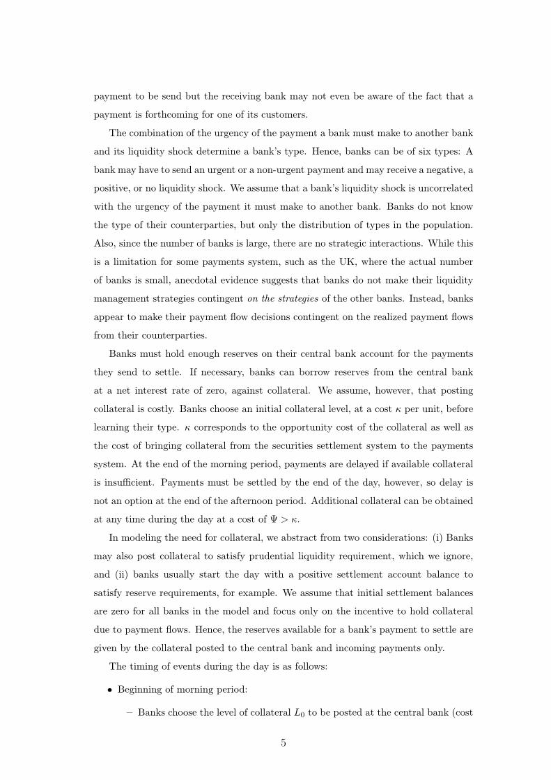
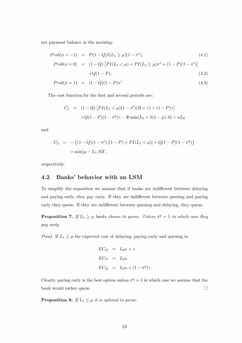
Figure 2 represents the two extreme cases that our model can accommodate. The

‘big box’ in that figure illustrates the case where the LSM can use all of the reserves

available in a bank’s reserve account. In other words a payment is released when there

is an incoming payment, regardless of the channel through which the incoming payment

is submitted. The same assumption is made in Martin and McAndrews (2008a). The

‘small box’ in the figure illustrates the case where the LSM cannot use any reserves

from the bank’s reserve account. In other words, a payment in the queue can only be

22

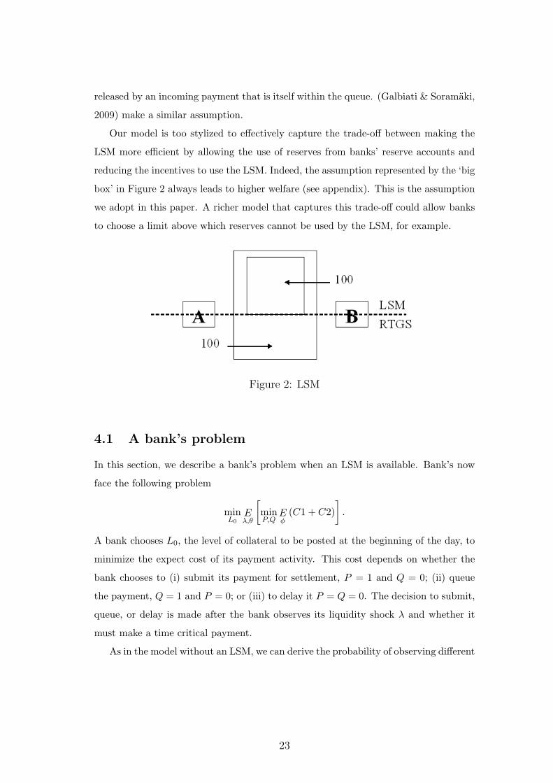
released by an incoming payment that is itself within the queue. (Galbiati & Soramaki,

2009) make a similar assumption.

Our model is too stylized to effectively capture the trade-off between making the

LSM more efficient by allowing the use of reserves from banks’ reserve accounts and

reducing the incentives to use the LSM. Indeed, the assumption represented by the ‘big

box’ in Figure 2 always leads to higher welfare (see appendix). This is the assumption

we adopt in this paper. A richer model that captures this trade-off could allow banks

to choose a limit above which reserves cannot be used by the LSM, for example.

Figure 2: LSM

4.1 A bank’s problem

In this section, we describe a bank’s problem when an LSM is available. Bank’s now

face the following problem

minL0

Eλ,θ

[minP,Q

Eφ

(C1 + C2)]

.

A bank chooses L0, the level of collateral to be posted at the beginning of the day, to

minimize the expect cost of its payment activity. This cost depends on whether the

bank chooses to (i) submit its payment for settlement, P = 1 and Q = 0; (ii) queue

the payment, Q = 1 and P = 0; or (iii) to delay it P = Q = 0. The decision to submit,

queue, or delay is made after the bank observes its liquidity shock λ and whether it

must make a time critical payment.

As in the model without an LSM, we can derive the probability of observing different

23

net payment balance in the morning:

Prob(φ = −1) = P (1−Q)I(L1 ≥ µ)(1− πs), (4.1)

Prob(φ = 0) = (1−Q)[PI(L1 < µ) + PI(L1 ≥ µ)πs + (1− P )(1− πi)

]+Q(1− P ), (4.2)

Prob(φ = 1) = (1−Q)(1− P )πi. (4.3)

The cost function for the first and second periods are:

C1 = (1−Q)[PI(L1 < µ)(1− πi)(R + γ) + (1− P )γ

]+Q(1− P )(1− πq)γ −Ψmin(L0 + λ(1− µ), 0) + κL0

and

C2 = −{(1−Q)(1− πi) [(1− P ) + PI(L1 < µ)] + Q(1− P )(1− πq)

}×min(µ− L1, 0)Γ,

respectively.

4.2 Banks’ behavior with an LSM

To simplify the exposition we assume that if banks are indifferent between delaying

and paying early, they pay early. If they are indifferent between queuing and paying

early they queue. If they are indifferent between queuing and delaying, they queue.

Proposition 7. If L1 ≥ µ banks choose to queue. Unless πq = 1 in which case they

pay early.

Proof. If L1 ≥ µ the expected cost of delaying, paying early and queuing is:

ECD = L0κ + γ

ECP = L0κ

ECQ = L0κ + (1− πq)γ

Clearly, paying early is the best option unless πq = 1 in which case we assume that the

bank would rather queue.

Proposition 8. If L1 ≤ µ it is optimal to queue.

24

Proof. If µ ≤ L0 < 1 banks will have L1 < µ only if they get a negative liquidity shock.

The expected cost of delaying, paying early and queuing in that case is:

ECR2,D = L0κ + γ + (1− πi)(1− L0)Γ,

ECR2,P = L0κ + (R + γ)(1− πi) + (1− πi)(1− L0)Γ,

ECR2,Q = L0κ + (1− πq)γ + (1− πq)(1− L0)Γ.

Note that ECR2,P −ECR2,Q = R(1− πi) + (πq − πi)(γ + (1−L0))Γ ≥ 0, since πq ≥ πi

(as shown in Section 6.1). Similarly, ECR2,D−ECR2,Q = πqγ +(πq−πi)Γ(1−L0) ≥ 0.

Therefore if µ ≤ L0 < 1 and a bank receives a negative liquidity shock it will queue its

payment.

If 2µ−1 ≤ L0 < µ and a bank receives a negative liquidity shock the expected costs

given different payment decisions are the same as above. If instead a positive liquidity

shock is received, L1 > µ. In that case according to Proposition 7 that it is optimal

to pay early unless πq = 1 in which case banks queue. If a bank receive no liquidity

shock the expected costs are:

EC3,D = L0κ + γ + (1− πi)(µ− L0)

EC3,P = L0κ + (R + γ)(1− πi) + (1− πi)(µ− L0)

EC3,Q = L0κ + (1− πq)γ + (1− πq)(µ− L0)

Again, as EC3,P − EC3,Q = EC2,P − EC2,Q ≥ 0 and EC2,D − EC2,Q = γπq + Γ(πq −

πi)(µ − L0) ≥ 0 it is optimal to queue. Therefore if 2µ − 1 ≤ L0 < µ and a bank

receives a negative or no liquidity shock it will queue its payment, while a bank with

a positive liquidity shock will pay early.

Similar steps show that the expected cost of queuing is smaller than delaying or

paying early if 1− µ ≤ L0 < 2µ− 1 or 0 ≤ L0 < 1− µ in which case regardless of the

liquidity shock banks will have insufficient liquidity to make a payment.

Intuitively, the probability to receive a payment if an outgoing payment is queued is

larger or the same as the probability to receive the payment if it is delayed. In addition,

by queuing banks can avoid the resubmission cost, which could realize if they submit

a payment for settlement without sufficient funds. Therefore, if banks have insufficient

funds queuing is better than delaying a payment or paying early.

Table 2 summarizes the optimal decision for different types of the banks under

different conditions.

25

Table 2: Optimal decision given λ, L0, and γ.L0 region λ Decision

-1 P or Q (if πq = 1)L0 ≥ 1 0 P or Q (if πq = 1)[R1] 1 P or Q (if πq = 1)

-1 Qµ ≤ L0 < 1 0 P or Q (if πq = 1)

[R2] 1 P or Q (if πq = 1)2µ− 1 ≤ L0 < µ -1 Q

L0 ≥ 1− µ 0 Q[R3] 1 P or Q (if πq = 1)

-1 Q1− µ ≤ L0 < 2µ− 1 0 Q

[R4] 1 Q-1 Q

0 ≤ L0 < 1− µ 0 Q[R5] 1 Q

-1 Q2µ− 1 ≤ L0 < 1− µ 0 Q

[R6] 1 P or Q (if πq = 1)

4.3 Equilibrium with LSM

Given the optimal behavior in Table 2 we can derive τs, τi, τq, and τd, where τs is the

fraction of banks that submit payment, P = 1, and have ‘sufficient’ collateral, L1 ≥ µ,

τi is the fraction of banks that submit a payment and have ‘insufficient’ collateral,

0 ≤ L1 < µ, τq is the fraction of banks that queue their payments, and τd the fraction

of banks that delay their payment, P = 0. Note, that τs + τi + τq + τd = 1. Table 2

shows that τi = τd = 0.

With the expressions for τs and τq, we can obtain the probabilities of receiving a

payment conditional on the bank’s collateral and payment decision, πs, πi, πq, and πd.

We again consider the two extreme cases of n = 2 and n →∞.

Let’s start with πi. If the payment cycle is of the length n=2, then πi = τs.

Meaning, that the only way I will receive a payment is if my counterparty is of type τs.

If a payment cycle is of length n=3, then there are two cases that I should consider:

(i) a bank sending a payment to me is of type τs, or (ii) it is of type τi or τq and the

bank receiving my payment is of type τs. Therefore, for the cycle of length n:

πi = τs + τs(τi + τq) + τs(τi + τq)2 + ...τs(τi + τq)n−2 =n−2∑k=0

τs(τi + τq)k

26

Clearly, if τi + τq < 1 and n →∞

πi =τs

τs + τd

The probability of receiving a payment, given that L1 ≥ µ and P = 1 also depends

on the length of the payment cycle. If the payment cycle is of length n = 2, πs = 1−τd.

Which is to say, that a payment will be received, unless a counterparty chooses to delay.

If n = 3, a payment will be received if (i) a bank sending me a payment is of type

τs, or (ii) a bank sending me a payment is of type τi or τq and the bank receiving my

payment is not delaying: πs = τs + (τi + τq)(1− τd) = τs + (τi + τq)τs + (τi + τq)2. For

the cycle of length n:

πs = (τi + τq)n−1 +n−2∑k=0

τs(τi + τq)k

Again, if τi + τq < 1 and n →∞

πs =τs

τs + τd

Similarly, we can derive the probability to receive a payment, given that I choose

to delay (P = 0), πd. If n = 2, πd = τs. for a cycle of length n = 3 the probability to

receive a payment is πd = τs + (τi + τq)τs. For the cycle of length n:

πd = π =n−2∑k=0

τs(τi + τq)k

We can derive an equilibrium value for Γ. First we need to find the probability that

none of the other banks have made a payment. Given the payment cycle length of n

this happens with the probability of (τd + τi + τq)n−1. Therefore

Γ =(τd + τi + τq)n−1

nΨ < Ψ. (4.4)

Now we can write the expected cost of banks:

ECR1 = L0κ

ECR2 = L0κ + (1− πq)γθπ

ECR3 = L0κ + (1− πq)(1− π)γθ + (1− πq)Γ(µ− π(2µ− 1)− L0(1− π))

ECR4 = L0κ + (1− πq)γθ + (1− πq)Γ(µ− L0)

ECR5 = (1− πq)(γθ + Γµ) + (1− µ)πΨ + L0(κ− (1− πq)Γ− πΨ)

27

4.4 Long payment cycle

For long payment cycle, n = ∞. If everybody queues, πq = 1. If not everybody queues,

πq = τsτs+τd

, but we know that nobody would find it optimal to delay. Therefore πq = 1

for large payment cycle as everybody with sufficient funds pays and those without

funds queue. Plugging πq = 1 into expected cost expressions above it is easy to see

that:

ECR1,R2,R3,R4 = L0κ

ECR5 = L0κ + (1− µ− L0)πΨ.

When comparing R1 to R4, the only factor is the cost of collateral. Hence banks

will prefer to choose the lowest level of initial collateral possible in these regions, 1−µ.

Next, notice that

ECR4 − ECR5 = (1− µ)(κ− πΨ).

We have assumed that κ < πΨ, so the expected cost associated with R4 is smaller

than the expected cost associated with R5 or R6, and banks choose L∗0 = 1− µ.

4.5 Short payment cycles

In case of a short payment cycles, n = 2, πq = τs + τq. But as can be seen from Table

2 since all banks either queue or pay early, the equilibrium probability to receive a

payment given that a payment is queued is πq = 1. Therefore banks with sufficient

collateral pay early and those with insufficient collateral queue. In equilibrium πq = 1.

As in the case of a long payment cycle the equilibrium collateral level is L∗0 = 1−µ.

4.6 Discussion

Our results show that an LSM allows banks to reduce their initial level of collateral,

in a collateral-based system. In that sense, we could also call it a collateral-saving

mechanism. In our model, an LSM prevents the situation where payments are stuck

in a cycle where every bank needs to receive a payment in order to have enough

collateral for its own payment to settle. In addition, the LSM allows banks to avoid

the reputational cost R. This benefit is a bit hardwired into our model as we assume

that payments that cannot settle through the RTGS stream have a cost that is different

from payments that do not settle in the LSM. This is meant to capture the fact that if

a bank reaches its collateral limit, it is unable to settle an unexpected urgent payment,

which can be costly. An LSM allows banks to settle payments while leaving reserves

28

available to settle unexpected payments. A richer model that capture this intuition

should deliver results that are similar to the results from our model.

In a fee-based system, an LSM provides banks with a form of insurance against hav-

ing to borrow from the CB. This consideration is less relevant here, because borrowing

from the CB is free once the fixed cost of the initial level of collateral is sunk. Another

interesting point to note is that an LSM completely eliminates delay in a collateral

based system. This is not the case in a fee based-system. In a fee-based system, banks

with a negative liquidity shock may prefer to delay in the hope that they receive a

payment in the morning which allows them to avoid borrowing from the CB. Because

the marginal cost of borrowing is zero in a collateral-based system, no bank has such

incentives.

5 The Planner’s problem

In this section, we study the planner’s problem. The planner can direct banks to

choose an action, conditional on a bank’s type, and aims to minimize the expected

cost of settlement. The planner’s allocation may differ from the equilibrium allocation

because the planner takes into account the consequences of a bank’s action on the

expected settlement cost of other banks.

5.1 RTGS with a long cycle

With a long cycle, the planner chooses either a relatively high level of collateral, and

makes all banks submit their payment early, or a relatively low level of collateral, and

makes all banks delay their payment.

If the planner chooses L0 = 2µ−1 and P = 1 for all banks, then all payments settle

in the morning. Indeed, banks with a positive liquidity shock have sufficient collateral

and the settlement of their payment allows the payments of banks with insufficient

collateral to settle as well. Hence, πi → 1 with a long payment cycle and therefore the

expected cost of banks is W (L0 = 2µ− 1) = (2µ− 1)κ.

If the planner chooses L0 < 2µ − 1, then we know that πi = 0, irrespective of the

actions of the banks. The best that can be achieved given in this case is to delay all

payments, so that W (L0 = 1− µ) = (1− µ)κ + γθ. So the planner chooses a low level

of collateral, L0 = 1− µ, and delay all payments if

(3µ− 2)κ > γθ.

29

Otherwise, L0 = 2µ− 1 and no payments are delayed.

With a long cycle, the expected cost of having to increase collateral during the day

is vanishingly small. For this reason, the planner focuses only on the initial cost of

collateral and on the cost of delay. In contrast to the equilibrium allocation, the planner

can direct a bank to submit a non-time-critical payment. This allows the planner to

achieve πi = 1 with only L0 = 2µ− 1 in initial collateral.

For some parameter values, the equilibrium and the planner’s allocation will be the

same. For example, we have seen in section 3.5 that banks will choose L0 = 1 − µ

if π = 1/2, R(1 − θ) > γ and (3µ − 2)κ > 12θγ and the planner chooses L0 = 1 − µ

if (3µ − 2)κ > θγ. In contrast, Atalay et al. (2008) report that for fee-based RTGS

systems the planner’s allocation cannot be achieved. In both collateral and fee-based

systems, excessive delay is responsible for any differences between the equilibrium and

the planner’s allocation.

5.2 RTGS with short cycles

We now turn to the case with short cycles. We first prove the following lemma.

Lemma 9. If a positive mass of banks has insufficient collateral, then the planner

always chooses to delay the non-time-critical payments of such banks.

Proof. First, we show that submitting these payments has no benefit. Consider a

bank with insufficient collateral, called bank A. If bank A’s counterparty has sufficient

collateral, then its payment will settle regardless of what bank A does. If bank A’s

counterparty has insufficient collateral, then its payment cannot settle, regardless of

that bank A does. Indeed, even if bank A submits its payment, the payment will not

be released as neither bank has sufficient collateral. Next, we observe that submitting

bank A’s payment has a positive expected cost, since there is a positive probability the

payment will not settle.

Now we consider the planner’s actions for different values of L0 ∈ {1−µ, 2µ−1, µ, 1}.

If the planner chooses L0 = 1, then all banks have sufficient collateral and the

expected cost is κ.

If the planner chooses L0 = µ, then a fraction π of banks has insufficient collateral

and Γ = πΨ/2. If the planner chooses to make banks with a negative liquidity shock

submit their payments, then the expected cost is

30

EC (L0 = µ,neg. shock submit) = µκ + π3(1− µ)Ψ/2 + π2θ(R + γ). (5.1)

If, instead, banks with a negative liquidity shock delay their time-critical payments,

then the expected cost is

EC (L0 = µ,neg. shock submit) = µκ + π3(1− µ)Ψ/2 + πθγ. (5.2)

Note that EC (L0 = µ,neg. shock submit) > EC (L0 = µ,neg. shock delay) if and

only if π(R+γ) > γ. This is the same condition as is faced by banks in equilibrium. This

is not surprising since we saw that with short cycles there are no strategic interactions

between banks with insufficient collateral.

If the planner chooses L0 = 2µ− 1, then a fraction 1− π of banks has insufficient

collateral and Γ = (1− π)Ψ/2. The planner can choose to make all banks, only banks

with positive or no liquidity shocks, or only banks with positive liquidity shocks, submit

their time-critical payments in the morning. If all banks submit their time-critical

payments early, the expected cost is given by

EC (L0 = 2µ− 1,no delay) = (2µ−1)κ+(1−π)2(1−µ)Ψ/2+(1−π)2θ(R+γ). (5.3)

If, instead, banks with a positive or no liquidity shock submit their time-critical pay-

ments, then the expected cost is

EC (L0 = 2µ− 1,neg. shock delay)

= (2µ− 1)κ + (1− µ)(1− π)2Ψ/2 + πθγ + (1− 2π)(1− π)θ(R + γ). (5.4)

Finally, if only banks with a positive liquidity shock submit their time-critical pay-

ments, then the expected cost is

EC (L0 = 2µ− 1,neg. and no shock delay) = (2µ−1)κ+(1−µ)(1−π)2Ψ/2+(1−π)θγ.

(5.5)

Here again, the choice made by the planner between submitting and delaying is the

same as the choice made by banks.

If the planner chooses L0 = 1 − µ, then all banks have insufficient collateral and

Γ = Ψ/2. In this case, the planner chooses to delay all payments and the expected

cost is

EC(L0 = 1− µ) = (1− µ)κ + γθ + (2µ− 1)Ψ/2. (5.6)

31

Depending on parameter values, the planner may choose any of these actions. While

the case with short cycles has more cases that the case with a long cycle, the main

conclusions are the same. For some parameter values, the planner’s and the equilibrium

allocations are the same, as is the case when L0 = 1− µ in both cases.

5.3 LSM

In a payment system with LSMs planner would choose L0 = 1−µ and would queue all

payments irrespective of the length of the cycle. W (L0 = 1− µ) = (1− µ)κ. Thus the

first best in a payment system with LSM dominates the first best of a payment system

without LSM.

Note that the planner’s allocation and the equilibrium allocation are the same with

an LSM. This is a stronger result than what Atalay, Martin, and McAndrews (2008)

obtained for fee-based systems. They show that the equilibrium allocation is the same

as the planner’s allocation for some, but not all parameter values.

6 Conclusion

This paper investigates the effects of introducing liquidity saving mechanisms (LSMs) in

collateral-based RTGS payment systems. We characterize the equilibrium allocations

and compare them to the allocation achieved by a planner. We develop a model closely

related to Martin and McAndrews (2008a), who consider fee-based RTGS systems, to

facilitate the comparison between our results and theirs.

In a collateral-based system without an LSM, the allocation in equilibrium can dif-

fer from the planner’s allocation. However, in contrast to fee-based systems described

by Martin and McAndrews (2008a), we find that for some parameter values the equi-

librium and the planner’s allocation are the same. When the cost of initial collateral

is sufficiently high, compared to the cost of delay, the planner chooses to minimize the

amount of initial collateral and makes all banks delay. In equilibrium, banks make the

same choice. When the equilibrium and the planner’s allocation differ, there is too

much delay in both fee- and collateral-based system.

We show that introducing an LSM always improves welfare in a collateral-based

system. This is in contrast to fee-based systems where Atalay et al. (2008) show that

an LSM can reduce welfare. In a fee-based system, an LSM can undo incentives to

send payments early because it offers banks a way to insure themselves against the

cost of borrowing at the central bank. In contrast, in a collateral-based system, the

32

cost of borrowing is paid at the beginning of the day and is sunk at the time banks

choose whether to submit, delay, or queue their payment. The LSM does not affect

the incentives of banks that have sufficient collateral and it encourages banks with

insufficient collateral to queue, instead of delay.

In a collateral-based system with an LSM, the equilibrium and the planner’s al-

locations allocation are the same for all parameter values. The LSM allows banks to

save on their initial collateral while providing incentives to queue their payment. The

LSM allows offsetting payment to settle with less collateral. This aligns the bank’s in-

centives with that of the planner. Atalay et al. (2008) show that in fee-based systems

the equilibrium and the planner’s allocation may differ, for some parameter values.

In a fee-based system, if liquidity shocks are large, the planner may want banks with

negative liquidity shocks to delay, rather than queue their payments. This is beneficial

if the cost of the induced delay is smaller than the reduction in borrowing cost from

the central bank. In a collateral-based system, the planner does not face this type if

incentives because the cost of collateral is sunk at the time banks learn their liquidity

shock.

33

7 Appendix

If a payment is submitted outside the queue, depending on liquidity, the probability of

receiving a payment is either πs or πi. What is the probability that given a submission

of a payment to the queue a payment from some other bank will be received? Let’s

denote such probability by πq.

If a payment cycle is of the length n = 2, then πq = τs + τq, which is to say that

given that I queue my payment, I will receive a payment if my counterparty also queues

or submits a payment with enough liquidity. If n = 3, then πq = τs + (τi + τq)τs + τ2q .

Which is to say that there are three cases: (i) a bank sending me the payment is of

type τs, (ii) it is of type τi or τq and the bank receiving my payment is of type τs, (iii)

everybody queues. For a payment cycle of the length n:

πq = τn−1q +

n−2∑k=0

τs(τi + τq)k

If not everybody queues, τq < 1, and payment cycle is very long, n →∞

πq =τs

τs + τd

How things would be different with an alternative LSM definition (small box in

Figure 2)?

πs = τn−1i +

n−2∑k=0

τsτki

πsn→∞ =

τs

τs + τq + τd

π =n−2∑k=0

τsτki

πn→∞ =τs

τs + τq + τd

πq = τn−1q

πq,n→∞ = 0, unless τq = 1, in which case πq = 1

πd =n−2∑k=0

τsτki

π0,n→∞ =τs

τs + τq + τd

Comparing the two alternatives, we can see that “big box” LSM leads to higher (or

same) probability to receive a payment compared to “small box” LSM for all bank

types!

Note, that πs ≥ πq ≥ π for the “big box” approach.

34

References

Angelini, P. (1998, January). An analysis of competitive externalities in grosssettlement systems. Journal of Banking & Finance, 22 (1), 1-18.

Angelini, P. (2000). Are banks risk averse? intraday timing of operations in theinterbank market. Journal of Money, Credit and Banking, 32 (1), 54-73.

Armantier, O., Arnold, J., & McAndrews, J. (2008). Changes in the timingdistribution of fedwire funds transfers. Economic Policy Review(Sep), 83-112.

Atalay, E., Martin, A., & McAndrews, J. (2008). The welfare effects of a liquidity-saving mechanism (Staff Reports No. 331). Federal Reserve Bank of NewYork.

Bech, M. L., & Garratt, R. (2003). The intraday liquidity management game.Journal of Economic Theory, 109 (2), 198-219.

Galbiati, M., & Soramaki, K. (2009). Liquidity saving mechanisms and bankbehaviour (Unpublished manuscript). Bank of England.

Kahn, C. M., & Roberds, W. (2001, June). The cls bank: a solution to the risks ofinternational payments settlement? Carnegie-Rochester Conference Serieson Public Policy, 54 (1), 191-226.

Martin, A., & McAndrews, J. (2008a, April). Liquidity-saving mechanisms.Journal of Monetary Economics, 55 (3), 554-567.

Martin, A., & McAndrews, J. (2008b). A study of competing designs for aliquidity-saving mechanism (Staff Reports No. 336). Federal Reserve Bankof New York, forthcoming Journal of Banking and Finance.

Roberds, W. (1999). The incentive effects of settlement systems: A compari-son of gorss settlement, net settlement, and gross settlement with queuing(Discussion Paper).

Willison, M. (2005). Real-time gross settlement and hybrid payment systems: acomparison (Tech. Rep.).

35