Finance and Economics Discussion Series Divisions of Research & Statistics and Monetary Affairs

Federal Reserve Board, Washington, D.C.

Liquidity, Default, Taxes and Yields on Municipal Bonds

Junbo Wang, Chunchi Wu, and Frank Zhang 2005-35

NOTE: Staff working papers in the Finance and Economics Discussion Series (FEDS) are preliminary materials circulated to stimulate discussion and critical comment. The analysis and conclusions set forth are those of the authors and do not indicate concurrence by other members of the research staff or the Board of Governors. References in publications to the Finance and Economics Discussion Series (other than acknowledgement) should be cleared with the author(s) to protect the tentative character of these papers.

Liquidity, Default, Taxes and Yields on Municipal Bonds

Junbo Wang, Chunchi Wu and Frank Zhang*

July 8, 2005

Abstract

We examine the relative yields of Treasuries and municipals using a generalized

model that includes liquidity as a state factor. Using a unique transaction dataset, we are able to estimate the liquidity risk of municipals and its effect on bond yields. We find that a substantial portion of the maturity spread between long- and short-maturity municipal bonds is attributable to the liquidity premium. Controlling for the effects of default and liquidity risk, we obtain implicit tax rates very close to the statutory tax rates of high-income individuals and corporations, and these tax rate estimates are remarkably stable over maturities.

* Junbo Wang and Chunchi Wu are at Syracuse University, and Frank Zhang is at the Federal Reserve Board in Washington DC. Address correspondence to Chunchi Wu, Whitman School of Management, Syracuse University, Syracuse, NY 13244. Tel: 315-443-3399, fax: 315-443-5457 and email: cwu@syr.edu. An earlier version of this paper titled “Inferring Marginal Tax Rates from Green’s Model with Default” was presented at the 2003 WFA Meeting in Cabo, Mexico. We thank Clifford Ball, John Chalmers, Pierre Collin-Dufresne, Cheng F. Lee, Suresh Sundaresan, Walter Torous, Rossen Valkanov, and Yuewu Xu for helpful comments. This paper represents the views of the authors and does not necessarily represent the views of the Federal Reserve Board or members of its staff.

1

The fixed-income securities market is an important segment in the U.S. financial

markets. This market has been particularly innovative and experienced considerable

growth recently. Not surprisingly, there has been extensive literature attempting to

explain the yield spreads between different fixed income securities. A subject that has

long intrigued financial researchers is how the yield spreads between tax-exempt and

taxable securities are determined. Are default and liquidity risk priced in municipal

bonds? What portion of these spreads is attributed to taxes, default, and liquidity risk?

These issues are fundamentally important from an investment perspective due to the

sheer size of the municipal market, which now approaches 1.9 trillion dollars.

Bond returns are subject to different tax treatments. Interest on municipal bonds

is exempt from federal income taxes though not necessarily exempt from state taxes. By

contrast, interest on Treasury and government agency bonds is subject to federal income

taxes but exempt from state income taxes.1 In equilibrium, one expects the after-tax

returns of taxable and tax-exempt bonds to be equal if both have same maturity and

comparable risk characteristics. The bond market thus provides an excellent financial

laboratory to evaluate the impact of taxation on the relative values of tax-exempt and

taxable bonds. The relative yields of taxable and municipal bonds should reflect the tax

rate of the marginal investor who is indifferent between these two bonds. Therefore, one

ought to be able to infer from the relative bond yields the implicit tax rate of the marginal

investor reasonably expected to hold these bonds.

Unfortunately, empirical evidence has not conformed very well to this expectation

but instead indicates that municipal bond yields are often higher than expected relative to

yields on U.S. Treasury bonds. This anomaly is more pronounced for long-maturity

2

bonds. The relatively high yields of municipal bonds imply a tax rate lower than

expected for the marginal tax rates of high-income individuals and corporations.

Moreover, the implied marginal tax rate is much lower for long-maturity municipal bonds

than for short-maturity bonds of similar quality and characteristics.

Several hypotheses have been advanced to explain the muni puzzle. The

institutional demand hypothesis suggests that the marginal tax rate is determined by

institutional trading activity (see Fortune, 1973; Galper and Peterson, 1971; Kimbal,

1977; Fama, 1997). Commercial banks can purchase municipals to shield their income

from taxes. An increase in their demand causes municipal yields to fall and the implicit

tax rate to rise. Since commercial banks prefer short-term bonds, the implicit tax rate

would tend to be high for these bonds relative to long-term bonds.2 Other explanations

for the yield curve anomaly include tax-timing options (Constantinides and Ingersoll,

1984), clientele effects (Mussa and Kormendi, 1979; Kidwell and Koch, 1983), and

changes in tax regimes (Poterba, 1989).

While the arguments above have some merit, it remains unclear whether they can

fully explain the anomalous behavior of municipal yield curves. In an important paper,

Green (1993) proposes an alternative model to explain the behavior of taxable versus tax-

exempt yields. A basic argument in this model is that high-tax investors generally prefer

portfolios of taxable bonds that are tax-advantaged (or tax-efficient) to individual taxable

bonds with similar pretax cash flows. In particular, they can avoid taxes on coupon

1 Unlike Treasuries and municipals, corporate bond interest is subject to both federal and state taxes. 2Along a similar line on institutional demand but with a different focus, Green and Odegaard (1997) indicate that many institutions such as pension funds are either not taxed at all or have much lower taxes than individuals. If any of these institutions invests heavily in long-term taxable bonds, the yield on long-maturity taxables will be lower. This will lower the yield spread between taxables and tax-exempts as well as the implicit tax rate.

3

income by constructing portfolios of taxable bonds that generate offsetting losses or

investment interest expenses. If these investors are marginal across these portfolios and

municipals bonds, they will apply the same discount factors to the after-tax cash flows

from both positions. Using this relationship, Green obtains investors’ implicit valuation

of the pretax cash flows from par taxable bonds. By appealing to the arbitrage activities

of dealers and tax-exempt institutions, he derives an equilibrium model to explain the

relative yields of taxable versus tax-exempt bonds. The intuition behind this model is

that investors holding both taxables and municipals may not regard coupon income as

fully taxable at the margin because of the offsetting investment interest elsewhere in their

portfolios. These implicit tax benefits tend to increase with maturity, thus pulling down

the yield curve of taxable bonds at the long end.

Empirical evidence shows that Green’s model explains a considerable portion of

the relative yield differences between taxable and tax-exempt bonds (see Green, 1993).

Chalmers (1995) finds that Green’s model cannot be rejected. However, although this

model replicates the differences in curvature between the taxable and tax-exempt yield

curves reasonably well, it continues to underestimate the long-term tax-exempt yields.3

Also, the predictive ability of the model does not hold up very well especially when there

are significant changes in statutory tax rates. While changes in tax regimes may be

blamed, these problems can also be caused by missing factors. Of particular concern is

that default and liquidity risk of municipal bonds are ignored in this model.

Municipal bonds are not risk-free and to some extent may even be riskier than

corporate bonds in the same rating class due to the unique features of municipal assets

and less predictable political processes (see Hempel, 1972; Zimmerman, 1977; and

4

Trzcinka, 1982).4 Although municipal bonds were traditionally considered to be only

second to U.S. Treasuries in safety, defaults on municipal bonds since the late 1970s,

along with other problems, have raised concern about the credit risk of municipal bonds.

For example, of the municipal bonds issued between 1977 and 1998, 1,765 out of a total

of 253,850 issues were defaulted, with a face value of $24.9 billion out of a total of

$375.5 billion (see Litvack and Rizzo, 1999). Thus, the probability of default may not be

trivial and is of potentially greater concern for low-rated uninsured municipals.

Empirical evidence on the role of default risk is inconclusive. Several studies

(e.g., Trzcinka, 1982; Yawitz, Maloney and Ederington, 1985; Scholes and Wolfson,

1992; Kim, Ramaswamy and Sundaresan, 1993; Stock, 1994; and Liu, Wang and Wu,

2003) show that credit risk differences explain the relative yields of taxable and tax-

exempt bonds.5 However, other studies (Gordon and Malkiel, 1981; Skelton, 1983; Ang,

Peterson and Peterson, 1985; Green, 1993; and Chalmers, 1998) find that differential

default risk cannot explain the municipal bond puzzle. A perplexing finding is that the

term structure of municipal bonds remains steeper than that of the U.S. Treasuries even

after the effect of default risk is controlled.

An important factor completely left out by previous municipal bond pricing

models is liquidity risk. The municipal market is very illiquid compared to the U.S.

Treasury bond market or the equity, futures and foreign exchange markets. Several

3 See Green (1993), p. 236. 4 Municipal assets cannot be seized as easily as corporate assets in bankruptcy proceedings because they may be physically difficult to seize or legally protected. In addition, the incentive problem or moral hazard is perceived to be more severe for municipalities. 5 Kim, Ramaswamy and Sundaresan (1993) provide a theoretical explanation for why default risk may cause the term structure to have a steeper slope. They argue that credit spreads for high-quality coupon bonds increase with maturity because longer bonds have more coupons subject to default risk. This relationship between the credit spread and term to maturity can also explain the higher relative yields of municipal bonds.

5

reasons have contributed to low liquidity in the municipal bond market. First, the

municipal bond market is a very thin market; many municipal bonds are traded only a

few times after issuance (see Downing and Zhang, 2004). Average weekly muni trading

volume is generally less than 12 percent of Treasury trading volume. On the other hand,

the number of muni bonds far exceeds Treasuries; well above one million different

municipal securities are issued by over 50,000 state and local governments (see Fabozzi,

1997). Thus, most individual muni bonds are traded infrequently. Second, the municipal

market is much less transparent in terms of the availability of basic information for

trading activity. Information for individual bond transactions has not been publicly

disclosed until very recently and comprehensive trade volume and price data were only

publicly available after a two-week lag.6 Third, the municipal bond market is also less

transparent in terms of information about the bond issuers because they are not subject to

the same financial disclosure requirements as are publicly traded corporations.7 Lack of

transparency considerably increases the information cost of trading and reduces

liquidity.8

Although it has been long recognized that the municipal market is illiquid and

liquidity risk is a potentially important determinant of municipal yields, few studies have

provided a quantitative assessment of the size of the liquidity risk premium. A primary

reason for the lack of empirical research is that reliable transaction data for municipal

bonds were virtually non-existent until very recently. Thus, how much municipal bond

6 Beginning in January 2005, the problem of lagged release in trading information has diminished. 7 Most municipal bond issuers only release detailed financial information when they float a bond, while publicly traded corporations are required to maintain a quarterly data feed on their activities (e.g., 10-Q and 10-K reports). 8 Harris and Piwowar (2004) report that the effective spreads in muni bonds average almost 2 percent of price for representative retail-sized trades (20,000 dollars) while the average yield to maturity is close to 6 percent.

6

yield is attributable to liquidity risk remains unclear. In this paper, we are able to

estimate the liquidity premium of municipal bonds by using the transaction database

recently made available by the Municipal Securities Rulemaking Board. As such, this

paper represents the first empirical study of the effect of liquidity risk on the relative

municipal bond yield curve using transaction data.

The model that we propose accounts for the effects of both liquidity and default

risk on the relative yields of taxable and tax-exempt bonds. Most studies on the liquidity

effect have focused on equity markets where transaction data are easily accessible. An

exception is Harris and Piwowar (2004), which examines transaction costs and trading

volume in the U.S. municipal bond market. Unlike their studies, we focus on the

sensitivity of municipal yields (or expected returns) to liquidity risk and examine its

effect on the equilibrium pricing of municipal bonds. Specifically, we investigate the

effect of systematic liquidity risk on bond yields instead of the level of liquidity cost per

se. We construct a broad liquidity measure for the municipal market along the line of

Pastor and Stambaugh (2003), which captures temporary price fluctuations induced by

order flow. By incorporating liquidity as an additional state factor in municipal bond

yields, we find that the explanatory power of the model is greatly improved.

Our empirical results show that the liquidity risk premium accounts for a

significant portion of municipal bond yields. Results suggest that investors require a

higher yield on those municipal bonds whose returns are more sensitive to aggregate

market liquidity. Within a rating class, the sensitivity of municipal yields to market-wide

liquidity increases monotonically with maturity. At the same time, controlling for

maturity, the sensitivity of municipal yields to market-wide liquidity increases

7

monotonically as the bond rating drops from AAA to BBB. Liquidity premium explains

about 7 to 13 percent of the observed municipal yields for AAA bonds, 7 to 16 percent

for AA/A bonds and 8 to 20 percent for BBB bonds with different maturities. Ignoring

the liquidity risk effect thus results in an underestimation of municipal bond yields.

Including liquidity risk in the pricing model also helps explain the municipal yield

curve anomaly. Long-maturity municipal yields are high relative to the equivalent after-

tax yields of Treasury bonds, partly due to liquidity risk. Our results show that the

liquidity risk premium alone accounts for 65 basis points (bps) for AAA bonds, 79 bps

for AA/A bonds and 111 bps for BBB bonds with 20-year maturity. In contrast, liquidity

risk premiums are only 14 bps, 16 bps and 23 bps for 1-year AAA, AA/A and BBB

bonds, respectively. Thus, the liquidity premium accounts for a substantial portion of the

maturity spread between 20-year and 1-year bonds. Controlling for the effects of default

and liquidity risk, we obtain implicit income tax rates very close to the statutory tax rates

of high-income individuals and corporations. More importantly, these implicit tax rates

are very stable when estimated from observed yields of bonds with different maturities.

Furthermore, our liquidity premium estimates are highly correlated with

traditional liquidity variables. We find that municipal bonds with high volume and

trading frequency and larger issue size have a low liquidity risk premium. Thus, the

Pastor-Stambaugh method, which we employ to construct the aggregate liquidity of the

municipal bond market, is quite effective in abstracting the liquidity feature of the bonds.

Overall, our results show that the generalized model with liquidity risk explains the

behavior of Treasury and municipal yield curves very well.

8

The remainder of this paper is organized as follows. Section I reviews the related

literature on municipal bonds. Section II proposes a generalized municipal bond model

to incorporate the effects of default and liquidity, and discusses the empirical

methodology. Section III describes the data sample and Section IV presents empirical

results for municipal bonds of different ratings, maturities and trading characteristics.

Finally, Section V summarizes major findings and concludes the paper.

I. Related Literature

Traditional models of the yield relationship between taxable and tax-exempt

bonds assume that investors are at the margin on all bonds. They can trade freely without

any friction, and the taxation of long and short positions is completely symmetric.

Investors apply the same discount factors to the after-tax cash flows from both taxable

and tax-exempt bonds. In addition, it is assumed that municipal bonds are default-free

and priced at par, and investors hold them to maturity. Given these conditions, it follows

that the yield on the tax-exempt bond (Mt) is simply equal to the yield on the taxable

bond (Ct) times one minus the marginal investor’s tax rateτ :

)1( τ−= tt CM (1)

Miller (1977) hypothesizes that in equilibrium, corporate capital structure

decisions will force the tax rate in (1) to be the top marginal corporate tax rate. Fama

(1977) predicts that the equilibrium tax rate equals the highest marginal corporate income

tax rate because banks were able to deduct interest expenses incurred to invest in

municipal bonds from their taxable income.

Empirical evidence has shown that the implied tax rates estimated from (1) are

considerably lower than the statutory tax rates for high-income individuals and

9

corporations, particularly for long-maturity municipals. There have been attempts to

explain this anomaly. The clientele hypothesis argues that long- and short-term bond

markets may be dominated by different groups of investors. Changing tax regimes can

also incur investment risk and affect bond values, particularly for long-maturity

municipals (see Poterba, 1989). Furthermore, inferior tax-timing options on municipal

bonds may raise the relative yields especially for long maturity municipals (see

Constantinides and Ingersoll, 1984).9

Trzcinka (1982) argues that ignoring the time-varying risk premium results in an

underestimation of the implicit marginal tax rate.10 He suggests including a random

intercept term in the yield relationship of (1) to capture the time-varying risk premium:

ttt CM βΛ += (2)

where tΛ is the time-varying risk premium and τβ −= 1 . In this model, tΛ is included

to allow for the differences in default risk between tax-exempt and taxable bonds.

Yawitz, Maloney and Ederington (1985) demonstrate that if two bonds have

different probabilities of default, β will depend on the relative magnitudes of these

probabilities and thus cannot be interpreted as an estimate of 1-τ. Specifically, they show

that in equilibrium the following yield relationship holds:

tttt CM βα += (3)

where ),1(1 g

t

tt τ

λλα −−

= andt

t λτβ

−−=

11 , tλ is the default probability at time t, τ is the

ordinary income tax rate and gτ is the capital gain (or loss) tax rate.11

9 An investor purchasing a taxable bond at a premium can amortize the premium against interest income over the remaining life of the bond. By contrast, the premium on a tax-exempt bond cannot be so amortized. In addition, capital gains from selling municipal bonds are subject to federal taxes.

10

Green (1993) proposes a different model that considers investors’ ability to shield

coupon income from taxation. Taxable investors may form a tax-advantaged portfolio to

avoid taxes on the cash flows received before maturity by the following trading strategy.

Suppose there is a par bond with coupon rate C and maturity date T and another par bond

with coupon rate C/2 and the same maturity date but traded at a discount. A long position

with two C/2 coupon bonds and a short with one C coupon bond will result in no coupon

income and hence, no net tax liability prior to maturity. This strategy can be applied to

any bonds with different coupons to form a tax-advantaged portfolio. While individual

investors may be precluded from holding this type of tax-advantaged portfolio due to

limitations on interest deductions from borrowings and short positions, bond dealers are

not. Therefore, from a dealer’s point of view, cash flows from par bonds and a sequence

of pure principal payments are equivalent. Any difference in price between a pair of

bonds or bond portfolios with identical income streams creates an arbitrage opportunity

for dealers.

Specifically, to the investor who pursues the above strategy to generate net zero

coupon payments, the after-tax cash flow of the position is )1(1 tP−−τ where tP is the

cost of the position at time t, which is equal to the total price of two C/2 coupon bonds

minus the price (=1) of one C coupon bond assumed equal to par. The price tP of this

position must then be equal to the discounted after-tax value of its cash flow:

ttt dPP )]1(1[ −−= τ (4)

where td is the after-tax discount factor. Solving for tP yields

10 A similar argument is made by Wu and Yu (1996) in a different context. 11 Wu (1991) extends Yawitz et al. (1985) to consider investors’ risk-averse behavior and finds that the slope coefficient further depends on risk premium.

11

t

tt d

dP

ττ

−−

=1

)1( (5)

From the dealer’s viewpoint, cash flows from par bonds with maturity T and a

sequence of pure principal payments are equivalent and so they should have the same

price; that is,

∑ +==

T

tTtT PPC

11 (6)

Substituting tP in (5) into (6) gives

T

T

t

tT

tT d

ddd

Cττ

ττ

−−

+−−

∑== 1

)1(1

)1(1

1 (7)

At the same time, the value of a par municipal bond with equal maturity will be equal to

∑ +==

T

tTtT ddM

11 (8)

Combining (7) and (8), one can obtain the following equilibrium relationship

between the yield curves of municipals and Treasuries:12

( )∑

−

∑−

−=

=

=

T

t T

t

T

t t

t

TT

dd

dd

CM

1

1

1

11

τ

ττ (9)

where ))1(1( t

tt P

Pd

−−=

τ is the after-tax discount factor for the cash flow at time t, and

tP is the pretax discount factor of a zero-coupon default-free taxable bond. The model

implies that the ratio of the tax-exempt yield to the taxable yield, MT/CT, increases with

maturity. When maturity T = 1, the ratio multiplying the after-tax coupon on the right

side of (9) is equal to one, and 1 – MT/CT gives the tax rate of the marginal investor. For

12

longer maturities, the ratio multiplying the after-tax coupon is greater than one if forward

rates are positive (dT < dt for t < T). The longer the maturity, the larger this ratio, making

MT increasingly large relative to CT. Thus, if one uses the formula 1- MT/CT to obtain the

implicit tax rate from the yields of taxable and tax-exempt bonds, the resulting estimate

will be biased downward.

While Green’s (1993) model is quite appealing, it does not consider the effects of

liquidity and credit risk. Unlike Treasury securities, municipal bonds are subject to

default. In addition, compared to the Treasury market, the municipal market is very

illiquid. These two factors can complicate the equilibrium yield relationship. Liu, Wang

and Wu (2003) consider the effect of default risk on municipal yields. They argue that

ignoring default risk may result in a biased estimation of the implicit marginal income tax

rate for long-maturity bonds. However, several studies have shown that for default risk

to explain the muni yield puzzle, the implied default probabilities for municipals would

have to be unreasonably large (see, for example, Poterba, 1986; Jordon and Jordan, 1990;

and Green, 1993). Chalmers (1998) uses a large sample of municipals over an extended

sample period to examine the issue and finds that default risk cannot explain the muni

yield puzzle. Thus, default risk alone does not appear to be able to provide the answer to

the empirical puzzle.

In this paper, we explore the role of liquidity risk in municipal bond pricing. We

take advantage of a unique transaction dataset recently made available by the Municipal

Securities Rulemaking Board to estimate the liquidity risk of municipals and examine its

effect on bond yields. To the extent that illiquidity can significantly affects the municipal

bond yields, analyzing the effect of liquidity risk should shed light on the muni puzzle.

12 See Green (1993) for the details of derivation.

13

In the following section, we propose a generalized municipal bond model with default

and liquidity risk and discuss the empirical estimation procedure.

II. A Generalized Municipal Bond Pricing Model

A. The Model

Following Green (1993), we assume that municipal and Treasury bonds are priced

at par and both are noncallable. In addition, investors pursue a buy-and-hold strategy.

However, unlike his model, municipal bonds are subject to default. The probability of

default at time t is tλ and the recovery rate is δ when default occurs.13

When there is no default, the present value of the payoff for the municipal bond is

( )∏ −⎟⎠⎞⎜

⎝⎛∑ +

==

T

tt

T

tTtT ddM

111 λ (10)

Conversely, when default occurs, the bond investor receives a residual (recovery) amount

δ. The present value of the expected cash flow of the municipal bond if default occurs at

time i, is given by

( )∏ −⎟⎠⎞⎜

⎝⎛ +∑

−

=

−

=

1

1

1

11

i

kki

i

ttT dM λλδ (11)

where δ is expressed in terms of present value. The value of the municipal bond at time t

is equal to the sum of (10) and (11). Because we assume that the municipal bond is

priced at par, the pricing formula can be written as

( ) ( )∑ ⎥⎦⎤

⎢⎣⎡ ∏ −⎟

⎠⎞⎜

⎝⎛ +∑+∏ −⎟

⎠⎞⎜

⎝⎛∑ +=

=

−

=

−

===

T

i

i

kki

i

ttT

T

tt

T

tTtT dMddM

1

1

1

1

111111 λλδλ (12)

Combining the pricing formula for Treasuries in (7) with (12), we obtain the following

equilibrium relationship between municipal and Treasury yields:

13 The recovery rate is formulated as a fraction of the face value.

14

( ) ( ) ( )

( ) ( )⎭⎬⎫

⎩⎨⎧

∑ ⎥⎦⎤

⎢⎣⎡ ∏ −⎟

⎠⎞⎜

⎝⎛∑+∏ −∑

−

−

∑ ⎥⎦⎤

⎢⎣⎡ ∏ −−⎥⎦

⎤⎢⎣⎡ ∏ −−

+∑−−

=

=

−

=

−

===

=

−

==

=

T

i

i

kki

i

tt

T

tt

T

tt

T

T

T

i

i

kki

T

ttTT

t t

tT

T

ddd

d

d

dd

CM

1

1

1

1

111

1

1

11

1

111

11

111

11

λλλτ

τ

λλδλ

ττ

(13)

The pricing formula above is not complete because it does not include the effect

of liquidity risk, which is considered to be a critical factor for municipal bond pricing.

Liquidity is perceived as an important feature of the investment environment. Previous

studies have shown that the level of liquidity affects expected asset returns (see, for

example, Amihud and Mendelson, 1986, 1991; Brennan and Subrahmanyam, 1996;

Brennan, Chordia and Subrahmanyam, 1998; and Amihud, 2002). That the level of

liquidity can affect transaction cost and asset price is not surprising. What is more

important is whether liquidity risk is a systematic risk that affects equilibrium asset

returns. In an influential paper, Pastor and Stambaugh (2003) show that expected stock

returns are significantly affected by systematic liquidity risk. They suggest that it should

be fruitful to examine the liquidity in the bond market and its impact on pricing, since the

effect of liquidity risk on bond returns can potentially be quite different from that on

stock returns.14

To account for the effect of liquidity risk, we add a liquidity risk variable to (13)

and rewrite it in a more compact form:

LCM LtTTT ββΛ ++= (14)

14 Recent studies in fixed-income markets have found that traditional term structure models of defaultable bonds explain only a small portion of yield spreads (see, for example, Huang and Huang, 2003). A potential cause is that liquidity risk is not accounted for by these models. Longstaff, Mithal and Neis (2005) find that the liquidity premium accounts for a significant portion of corporate bond spreads. Since

15

where

( ) ( )

( ) ( )⎭⎬⎫

⎩⎨⎧

∑ ⎥⎦⎤

⎢⎣⎡ ∏ −⎟

⎠⎞⎜

⎝⎛∑+∏ −∑

−

−

∑ ⎥⎦⎤

⎢⎣⎡ ∏ −−⎥⎦

⎤⎢⎣⎡ ∏ −−

=

=

−

=

−

===

=

−

==

T

i

i

kki

i

tt

T

tt

T

tt

T

T

T

i

i

kki

T

ttT

T

ddd

d

d

1

1

1

1

111

1

1

11

111

11

111

λλλτ

τ

λλδλ

Λ

and

( )

( ) ( )⎭⎬⎫

⎩⎨⎧

∑ ⎥⎦⎤

⎢⎣⎡ ∏ −⎟

⎠⎞⎜

⎝⎛∑+∏ −∑

−

∑−−

=

=

−

=

−

===

=

T

i

i

kki

i

tt

T

tt

T

tt

T

T

t t

t

T

ddd

dd

1

1

1

1

111

1

111

111

λλλτ

ττ

β

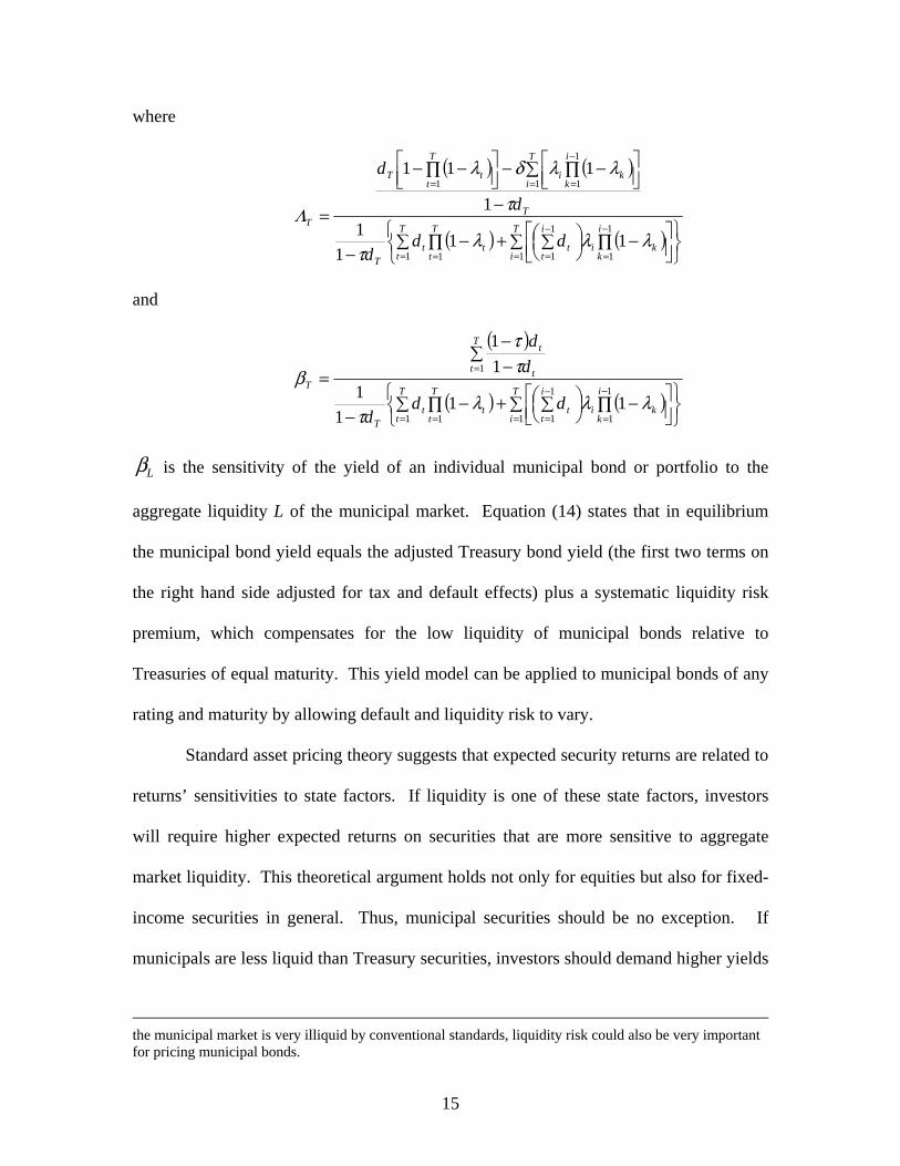
Lβ is the sensitivity of the yield of an individual municipal bond or portfolio to the

aggregate liquidity L of the municipal market. Equation (14) states that in equilibrium

the municipal bond yield equals the adjusted Treasury bond yield (the first two terms on

the right hand side adjusted for tax and default effects) plus a systematic liquidity risk

premium, which compensates for the low liquidity of municipal bonds relative to

Treasuries of equal maturity. This yield model can be applied to municipal bonds of any

rating and maturity by allowing default and liquidity risk to vary.

Standard asset pricing theory suggests that expected security returns are related to

returns’ sensitivities to state factors. If liquidity is one of these state factors, investors

will require higher expected returns on securities that are more sensitive to aggregate

market liquidity. This theoretical argument holds not only for equities but also for fixed-

income securities in general. Thus, municipal securities should be no exception. If

municipals are less liquid than Treasury securities, investors should demand higher yields

the municipal market is very illiquid by conventional standards, liquidity risk could also be very important for pricing municipal bonds.

16

(or expected returns) from holding municipals to compensate for this risk. Likewise, in

the domain of municipal securities, those municipals whose returns have higher

sensitivities ( Lβ ) to aggregate market liquidity should offer higher yields than other

municipals with lower sensitivities.

Intuitively, the role of liquidity in securities pricing would depend on the

importance of liquidity for a specific investment and the liquidity condition of a market

relative to others. Since the municipal market is relatively illiquid compared to other

markets, liquidity risk would likely be an important pricing factor for municipal bonds.

When there is a widespread deterioration in liquidity, it will be more difficult to liquidate

municipal bonds than Treasuries securities. In anticipation of costly liquidation in a low

liquidity environment, investors will require higher yields to compensate for this risk

regardless of the tax-exempt advantage of municipals. Furthermore, the trade size of

municipals is typically larger than that of equity transactions. Liquidity is expected to be

more valuable for investors trading large orders than small orders even in routine

transactions. In an unusual situation when the aggregate market liquidity dries up, it will

be much more difficult to trade large quantities. Taken together, liquidity risk should be

more serious concern for municipal investors and if so, this would have a significant

implication for municipal bond pricing.15

The relevance of liquidity risk to municipal bond pricing is measured by the

sensitivity coefficient Lβ to the aggregate liquidity of the municipal bond market.

Similar to the risk measure in traditional asset pricing models, Lβ captures the systematic

15 The importance of liquidity is well spelled out by the recent event associated with the reduction in personal taxes on regular income and dividends by the Bush Administration. The event triggered a sell-off

17

risk (liquidity beta) of individual municipal bonds to the market-wide liquidity. We use

the aggregate liquidity measure of the municipal market itself to estimate liquidity beta

for the following reasons. First, since an individual financial market typically exhibits

commonality in liquidity, it justifies the estimation of systematic liquidity risk of a

municipal bond by its co-variation with the liquidity innovations of the overall municipal

market. The rationale is that those municipal securities whose returns are more exposed

to market-wide liquidity fluctuations should have higher yields (expected returns).

Second, the Treasury yield (Ct) on the right hand side of the model in (14) has impounded

the effect of the Treasury liquidity risk and so there is no need to add the liquidity

innovations of the Treasury market as an additional explanatory variable in the municipal

yield model.

To estimate liquidity risk Lβ , we need to construct a market-wide liquidity

measure (L) for municipal bonds. In the following, we outline the procedure for

constructing a measure of aggregate liquidity for the municipal bond market in the spirit

of Pastor and Stambaugh (2003).

The proposed aggregate liquidity measure captures temporary price changes

associated with order flow. The fundamental argument is that lower liquidity tends to

correspond to stronger price reversals on the next trading day, resulting from the order

flow in a given direction on a particular day. For example, in the absence of private

information, a large number of sell orders (or a high sell volume) on a particular day will

cause a greater price rebound on the next trading day. This dimension of liquidity can be

gauged by the response of municipal returns in the next trading day to the signed volume

in the municipal market as the tax-advantage of municipals was eroded. Because liquidity was low, the sell-off had a tremendous impact on municipal bond prices across the board.

18

in the preceding trading day. Specifically, the liquidity measure for a bond in a month t

is the least squares estimate of the parameter t,iπ associated with the signed volume in

the following regression:16

tjitjie

tjititjie

tji uVolrsignrr ,1,,,,,,,,10,1, )( ++ +⋅++= πρρ (15)

where tjbtjie

tji rrr ,,,,,, −= is the return of municipal bond i on day j, tjir ,, , in excess of the

equally weighted municipal market return, tjbr ,, ; )( ,,e

tjirsign is the signed indicator which

is equal to 1 if etjir ,, is positive, and -1 if it is negative; and t,j,iVol is the dollar volume (in

ten-thousand dollars) for bond i.17 In this model, the order flow is measured by volume

signed by the contemporaneous excess return on a particular municipal security. The

order flow is expected to be followed by a return reversal if the municipal security is not

perfectly liquid. Presumably, the greater the expected reversal for a given dollar volume,

the lower the liquidity of the municipal security; that is, t,iπ is negative. The model in

(15) is estimated for individual bonds each month t using daily return and volume data.

In empirical investigation, in order to obtain a reliable estimate of π , we select in each

month only those bonds which have more than 10 observations.

The liquidity measure of each individual bond is then aggregated over all

municipal bonds (N) in the sample month by month:

∑==

N

1it,it N

1ˆ ππ (16)

Systematic liquidity risk, Lβ , is measured as the sensitivity of bond returns to unexpected

innovations in market-wide liquidity. To obtain the unexpected liquidity innovations

16 For the detail of the derivation, see Pastor and Stambaugh (2003).

19

( te ), we estimate the following autoregressive model for the differenced liquidity

measure:

t1t21t10t eˆaˆaaˆ +++= −− ππ∆π∆ (17)

The above regression is essentially a second-order autoregression in the level series of

market-wide liquidity.18 Since the residual term for municipal bond liquidity is typically

quite small, we multiply the estimated te by 100:

tt eL ˆ100 ⋅= (18)

After constructing the market-wide liquidity measure, we include it as a state factor for

the municipal bond yield model to estimate the liquidity risk premium of municipal

bonds.

B. Estimation Procedure

The municipal yield model in (14) can be estimated by the nonlinear regression

method. Since municipal bond yields are serially correlated, we correct the effect of

autocorrelation. The first step in empirical investigation is to abstract the liquidity

measure from (15) and (17). The model in (15) is particularly suitable for our

investigation of municipal market liquidity because it requires only the excess return and

dollar volume data. These data are readily available from the transaction records

provided by Municipal Securities Rulemaking Board (MSRB). As noted, to construct a

meaningful liquidity index, we impose the restriction of a minimal number of 10

transactions each month for an individual municipal security. Although municipals are

traded less frequently, this presents little difficulty because the MSRB database contains

17 Pastor and Stambaugh (2003) find that this specification works better than other specifications with excess lagged returns. 18 Pastor and Stambaugh (2003) show that this time-series model captures liquidity innovations rather well.

20

records for more than one million municipal securities. This large database grants us a

considerable leeway to choose a suitable sample to estimate market-wide liquidity. After

imposing the constraint of the minimal number of transactions per month, we still have

149,666 bonds that meet this criterion. This sample size is large enough to represent the

overall municipal market. Note that this particular sample is selected mainly for

estimation of the market-wide liquidity factor. For the estimation of the municipal yield

model in (14), we impose different criteria to better control the data sample as explained

later in the data section.

In the second step, we form the portfolios of muni bonds by rating and maturity.

There are advantages of estimating the yield model with portfolios. First, forming

portfolios allows us to construct more regular time series of municipal yields for

regression estimation, to overcome the problem of infrequent trading. Second, portfolio

formation reduces data noise associated with individual bonds due to recording errors and

stale prices. Because the portfolios are grouped by rating and maturity, we retain control

on these two important bond characteristics. We calculate the yield for each portfolio

from our data sample month by month. We then estimate the nonlinear model in (14)

using monthly yield data of each portfolio using the Gauss-Newton method.

III. Data Description

We use the municipal bond database provided by the Municipal Securities

Rulemaking Board in our empirical estimation. The MSRB is the self-regulatory agency

established by Congress, which develops rules subject to SEC approval to govern the

conduct of brokers and dealers involved in underwriting and trading municipal securities.

Approximately 2,700 municipal securities brokers and dealers are registered with the

21

MSRB. Since 1997, the municipal bond industry has operated under a mandatory

transaction reporting system overseen by the MSRB. All dealer-to-dealer and dealer-to-

customer muni bond transactions are reported to the MSRB after the close of business

each day. The MSRB then consolidates the daily reports. Beginning in July 2000, the

MSRB started releasing electronic files containing all municipal bond transaction data

two weeks after actual transactions took place.19 The MSRB transaction reports contain

data fields including CUSIP, security description, issue date, coupon, maturity date, trade

date, time of trade, par amount of trade, transaction price, and yield. Useful features of

the data include whether a transaction is sale to customer, purchase from customer or

inter-dealer trade, and an indicator showing whether the trade occurs before the syndicate

settlement date.

Additional information on the characteristics of each bond are collected from

Bloomberg, which includes the rating of a bond when it was issued, the issue size and

type (e.g., general obligation or revenue bonds), whether the bond is callable or contains

a sinking fund provision, and whether the bond is insured. Zero-coupon Treasury yields

are obtained from the Federal Reserve Board (FRB), where spot rates are estimated from

Treasury prices using the Svensson method (see Bolder and Streliski, 1999, for details).

The sample period is from July 2000 to June 2004. The initial sample contains a

total of 1,056,774 bonds, 27,330,633 transactions and dollar volume of 11.7 trillion. A

notable feature of the municipal market is that most bonds are not frequently traded.

Compared to the Treasury market, the trading volume on the municipal bond market is

19 The initial lag was one month, but the MSRB has since sequentially reduced the lag time to two weeks, one week and one day. Beginning January, 2005, the lag was substantially reduced as the MSRB and the Bond Market Association (BMA) partnered to make transaction data available within fifteen minutes of a trade.

22

much smaller. For example, in June 2004, the average weekly volume (total par value

traded) on the municipal market is 89.68 billion, while the average weekly Treasury

transaction is 756.21 billion, according to New York Fed’s weekly survey on primary

Treasury dealers conducted each Wednesday. Infrequent trading is a key factor

contributing to low liquidity in this market.

To construct the data sample for our empirical estimation of the municipal yield

model in (14), we match the raw MSRB data with bond characteristic information from

Bloomberg and impose the following screening criteria.20 We first drop trades that occur

on or before the underwriting syndicate settlement date, and keep only secondary market

trades. This filter reduces the number of bonds to 805,510 and the number of transactions

to 22,967,938. We then eliminate bonds with unknown credit ratings, leaving 686,859

bonds and 21,554,555 trades in the sample. Since our municipal model holds for straight

bonds, we delete bonds with embedded option features (i.e., bonds with call and sinking

fund provisions). Due to the fact that the majority of municipal bonds are callable, this

filter decreases the sample substantially to 114,626 bonds and 2,149,008 trades. We also

eliminate bonds that carry variable rates or irregular coupons. This restriction removes

185 bonds and 2,500 transactions. To focus on bonds that are relatively frequently traded

in order to construct the portfolios with enough observations, we keep only those

transactions that are within one year from the issuance date. This step excludes 61,371

bonds and leaves 53,070 bonds and 883,753 transactions in the sample. In addition, we

throw away transactions with obvious errors in prices or with missing prices. This filter

drops 207 bonds and 7,541 trades. Finally, for a similar concern about liquidity, we

23

exclude those bonds that are less than six months away from maturity. Our final sample

contains 48,278 bonds with a total of 753,268 secondary market transactions.

We group the individual bond data according to their ratings and maturities.

Because there are very few speculative bonds in our data sample, we include only bonds

in the following rating classes: AAA, AA/A and BBB. In the original database, AA and

A bonds are grouped together and so we keep them in one group. There are very few

trade and transaction price data for bonds with long maturity. We therefore lump

(equally weighted) all bonds with maturities from 18 to 22 years to form long-term

portfolios. This enables us to assemble a larger number of observations in portfolios to

examine the empirical properties of long-term municipals. The average maturity for these

long-term portfolios is very close to 20 years: 19.9 years for AAA, 19.5 years for AA/A

and 19.9 years for BBB bonds.21 For convenience, these portfolios are placed under the

20-year category for the corresponding rating class.

Table I provides the summary statistics for the three rating groups of municipals,

and Treasuries by maturity. Panel A shows that yields of AAA bonds are lower than

those of AA/A bonds which, in turn, are lower than those of BBB bonds. Yields of

Treasury bonds with the same maturity are generally greater than those of AAA and

AA/A bonds. However, Treasury yields may be lower than BBB yields, indicating that

the default and liquidity premia may outweigh the tax-exempt advantage for bonds in this

rating class. Figure 1 plots the time-series of municipal and Treasury yields for

maturities from one to ten years.

20 As noted earlier, this sample selection procedure applies to our yield model estimation. For the construction of the liquidity index, we impose a less stringent restriction that only requires a minimum of 10 transactions per month for each individual bond.

24

Panel B of Table I shows monthly averages of the number of transactions, trading

volume (in par amount), and the number of bonds for each rating-maturity portfolio. For

each month we calculate the number of bonds and transactions, and total par volume for

each portfolio and then average them over all months in the entire sample period. As

shown, the AA/A bonds have the largest number of transactions, volume and number of

bonds for most maturity groups, followed by AAA and BBB bonds. In terms of the

number of transactions, the five-year maturity bonds are highest whereas bonds in the 20-

year maturity group are lowest.

Panel A of Table II summarizes the yield spreads between Treasuries and AAA

bonds, between AAA and AA/A bonds and between AA/A and BBB bonds. Average

differences between Treasury and AAA yields are around 70 basis points. Average yield

differences between AA/A and AAA bonds, and between BBB and AA/A are about 10

and 50 basis points, respectively. The term structure of the yield spread between

Treasuries and AAA bonds exhibits a hump shape. The spread declines beyond the five-

year maturity, which confirms the previous finding that prime municipal bond yields rise

relative to Treasury yields when maturity gets longer (see Green, 1993).

Panel B reports term premiums for Treasuries and municipals. The term premium

is obtained by subtracting from the yield for a given maturity the corresponding yield of

one-year maturity. Consistent with previous findings, average yields for Treasuries

increase less rapidly with maturity than do those of municipals. However, average term

premiums are only higher for the 20-year municipal group relative to Treasury bonds.

This is somewhat different from previous findings, suggesting that the relative steepness

21 The shape of the yield curve between 18 and 22 years is close to linear and so an equally weighted average yield is very close to the average yield of 20-year bond.

25

of the yield curves may vary by sample periods. By contrast, average term premiums for

AAA municipals are higher than those for BBB municipals at all maturities. The

columns reporting the minimum values of the term premium show negative numbers for

Treasuries at all maturities whereas they are all positive for municipals. Results show

that while the yield curves of Treasuries may revert, this phenomenon has never occurred

for municipal bonds.

IV. Empirical Results

A. Estimation of the Municipal Yield Model

We next estimate the municipal yield model using the monthly yield series for

each maturity-rating group. Estimating the municipal bond yield model requires spot

rates of pure discount bonds. The pretax discount factor tP embedded in the after-tax

discount factor td at time t is the inverse of one plus the spot rate of a pure discount bond

to the power of t. We can express the after-tax discount factor td as a function of the

pretax discount factor tP and the marginal income tax rate. By substituting the definition

of the after-tax discount factor ))1(1/( ttt PPd −−= τ into the model and using the spot

rate data obtained from the FRB, we can directly estimate the marginal income tax rate

and default probability from the observed municipal and Treasury bond yields. The

nonlinear municipal yield model is estimated for bond groups with different ratings and

maturities.

In addition to spot rates, we need to construct the aggregate municipal bond

market liquidity index before estimating the yield model. We estimate liquidity measures

for individual bonds each month using the regression model in (15) and aggregate them

over all bonds to obtain the monthly series of the municipal market liquidity index.

26

Panel A of Figure 2 plots the estimates of the aggregate liquidity index for the

muni market. By construction, negative liquidity index values imply positive liquidity

costs. The aggregate liquidity measure shows occasional downward spikes. The largest

downward spike occurs in September 2001 when the market was shut down due to the

terrorist attack at the New York World Trade Center. The second largest spike occurs in

the fall of 2002 when the market was jittered by the episode of WorldCom. The third

largest spike occurs around July 2001 when the Enron scandal began to unravel. Another

major downward spike occurs after the announcement of the tax cut by the Bush

Administration on May 23, 2003, which triggers a sell-off in the municipal bond market

as the tax-exempt advantage of municipals is eroded.22 Overall, the aggregate liquidity

measure constructed from the Pastor-Stambaugh method appears to pick up significant

events quite effectively.

The median value of the aggregate liquidity measure is -2.37%. Excluding the

extreme value of September 2001, the mean liquidity index is -3.66%. These numbers

suggest that the average liquidity cost is around 2.4% to 3.7%, which represents the cost

for a $10 thousand trade in constant “municipal bond market” dollars of year 2000. The

correlation between the liquidity measure and the aggregate municipal bond market

return is 0.05, indicating that the liquidity cost is somewhat lower when the market

performance is better.

22 According to the tax bill passed May 23, 2003, the highest income tax rate for individuals is reduced to 35% retroactive to January 1, 2003. The next three rates are 33%, 28% and 25%. This tax act accelerates the tax reduction scheduled for 2004 through 2006 by the Economic Growth and Tax Relief Reconciliation Act of 2001. The new tax law also increases the taxable income level for the 10% bracket. Other effects of the 2003 tax act include child tax credit, marriage tax breaks, alternative minimum tax, business bonus depreciation and small-business spending (see the report of the Wall Street Journal May 23, 2003).

27

Panel B of Figure 2 plots the innovations of the liquidity measure. The

innovation series appears to be serially independent. The autocorrelation of innovations

of the liquidity measure is -0.114, which is relatively small. We employ this innovation

series in the nonlinear regression model to capture the effects of unanticipated liquidity

shocks on yields of municipal bonds.

Table III reports the estimates of the generalized municipal bond model with

liquidity risk.23 Parameter estimates for tax rate and default probability are expressed in

percentage terms, and standard errors are reported in parentheses. The estimates of the

liquidity risk parameter are very significant and of a negative sign. Since the liquidity

measure L also has a negative sign, the negative coefficient of the liquidity factor

translates into a positive effect on municipal bond yields. The sensitivity of municipal

bond yields to the liquidity factor increases significantly with maturity, suggesting a

much higher liquidity risk for longer-term bonds. For example, the liquidity risk

coefficient in absolute value for 10-year bonds is more than three times that of one-year

bonds for each rating class. This difference is even more striking for the 20-year bond

group. Moreover, the sensitivity of yields to liquidity increases as credit risk increases,

indicating that lower quality bonds have higher liquidity risk. This result lends support to

the contention of a positive correlation between credit and liquidity risk.

The estimates of marginal income tax rate and default parameter are all highly

significant. The estimated marginal tax rates are around 32 to 33 percent. Two

interesting patterns are observed. First, the estimates of implicit tax rates are very close

to the maximum statutory income tax brackets of high-income individuals and

23 The recovery rate is set equal to 0.4 whose value is very close to that used by Duffee (1999) and Elton et al. (2001).

28

corporations. Second, these implicit tax rate estimates are very stable over maturities.

These findings contrast sharply with previous findings that the implicit tax rates are

substantially below the statutory tax rates of high-income individuals and corporations,

and that the estimates of the implicit tax rate declines drastically with maturity. In some

studies, the estimated implicit income tax rates for municipal bonds with maturity longer

than 20 years are merely half of that for one-year municipal bonds.24 By contrast, our

empirical estimates do not exhibit these anomalies in the implicit income tax rates.

Results suggest that the so-called municipal yield puzzle may well be attributable to

missing factors in the traditional models.

The estimates of default probabilities are consistent with ratings. These estimates

are annualized default probabilities. The implied default probabilities are in line with

previous estimates.25 Given maturity, estimated default probabilities increase

monotonically as the rating decreases. Within each rating class, the default probability

estimates exhibit an upward trend with maturity. The upward-sloping term structure of

the default probability is consistent with empirical evidence on investment-grade bonds.

Overall, the model with liquidity risk explains the relative yield curves of

municipal bonds very well. The goodness-of-fit in terms of high R2 is quite good across

all ratings and maturities. The results suggest that personal taxes, liquidity and default

risk are important determinants of municipal bond yields.

B. Decomposition of Municipal Bond Yields

The results above show significant effects of liquidity risk on municipal bonds of

different ratings and maturities. A question of particular interest is how much municipal

24 See Table 3 in Green (1993, p. 239). 25 See, for example, Yawitz et al. (1985).

29

bond yield can be attributed to liquidity risk. The yield model allows us to separate the

effect of liquidity risk from the combined effect of personal taxes, default risk and

riskfree (Treasury) rates, which is nonlinear in nature due to the interactive effects among

these variables. We first employ the parameter estimates of default probability, tax rates

and liquidity risk to calculate the municipal bond yields. We then separate these

municipal bond yield estimates into the liquidity and non-liquidity components.

Table IV reports the results of yield decomposition, where the estimate of each

spread component is expressed in magnitude (%) and in the proportion of the observed

yield (% yield) for each yield component. We report the yield components for each

rating and maturity group. In addition, both observed yields and total yield estimate (the

sum of liquidity and non-liquidity components) are reported in the leading column of

each rating class.

The liquidity component of municipal yields increases with maturity and credit

risk in terms of both the magnitude and proportion of observed yields. The liquidity

spread in basis points increases from 14 to 65 for AAA bonds as maturity rises from one

to 20 years. Correspondingly, the liquidity spread in the proportion of the observed yield

increases from 7 to 13 percent. For AA/A bonds, the liquidity spread increases from 16

to 79 bps, which accounts for about 7 to 16 percent of the observed yields of different

maturities. For BBB bonds, it increases from 23 to 111 bps, or about 8 to 20 percent of

the observed yield. The results show that the amount of liquidity premium is sizable for

most bonds and it is particularly large for lower-quality long-term municipal bonds.

The non-liquidity yield component (including effects of taxes, default and risk-

free rates) also increases with maturity and credit risk. This increase is associated more

30

with the change in default risk than with taxes since the estimates of marginal tax rates

are not materially different over maturities and across ratings. As maturity increases, the

probability of default increases for these investment-grade municipal bonds. Similarly,

as the rating decreases, default probability increases. Since the default probability has a

positive effect on municipal yield, this increase in default probability contributes to the

increase in the non-liquidity yield component.

However, the non-liquidity yield component in percentage terms declines over

maturities. Although the non-liquidity yield component increases in magnitude with

maturity, observed yields appear to increase faster, due to an increase in liquidity risk as

maturity gets longer. As a result, the proportion of the non-liquidity component to the

observed spread declines with maturity. By contrast, the proportion of the liquidity

component to the observed spread increases with maturity.

This finding suggests that liquidity risk is a more important factor contributing to

the rising maturity premium of municipals relative to Treasuries. The liquidity premium

accounts for a substantial portion of the maturity premium. For example, as shown in

Panel B of Table II, the maturity premium for AAA bonds is 34 bps for two-year bonds

and 298 bps for 20-year bonds, a difference of 264 bps. In contrast, the corresponding

maturity premium for Treasuries increases from 41 to 277, a 236 bps difference. It

appears that the maturity premium increases faster for long-maturity municipal bonds.

But if we adjust the maturity premium of 20-year municipals by the incremental liquidity

premium of 48 bps (65-17 bps), we come up with an adjusted maturity premium of only

216 bps, which is lower than the corresponding maturity premium increase of

31

Treasuries.26 Thus, it seems that liquidity risk is the driving force behind the high yields

of municipals relative to Treasuries at long maturity. Chalmers (1998) finds that

differential default risk alone cannot explain the municipal yield puzzle. Our results are

consistent with this view.

C. Likelihood Ratio Tests

We next conduct the likelihood ratio test to see if liquidity risk adds significant

explanatory power to the municipal bond model. It is straightforward to perform the

likelihood ratio test on the incremental explanatory power of liquidity risk. The test

statistic is

)/(/)(

KnSSRkSSRSSRLR U

UC

−−= (19)

where SSRC is the sum of the squared residuals of the constrained model, which imposes

the condition that 0=Lβ , SSRU is the sum of the squared residuals of the unconstrained

(full) model, K (= 3) is the number of explanatory variables, k (= 1) is the number of

coefficients restricted to be zero, and n (= 48) is the number of observations. The test

statistic LR of the nonlinear yield model follows an F distribution with (k, n-K) degrees of

freedom if the disturbance term is normal under the null hypothesis that the restricted

coefficients are zero (see Gallant, 1987).27

Table V reports the results of likelihood ratio tests. The critical F value is 4.0 at

the five percent level. Results show that likelihood ratio tests reject the null hypothesis of

0=Lβ for all maturity-rating groups. Consistent with the t-tests in Table III, results

show that liquidity risk adds significant explanatory power to the municipal model.

26 This calculation assumes that Treasury bond’s liquidity risk is negligible and so it may overstate the effect of municipal liquidity risk. However, the qualitative effect of municipal liquidity risk holds true.

32

Thus, the effect of liquidity risk should be incorporated into the model in order to better

explain the behavior of the relative municipal-Treasury yield curves.

D. Liquidity and Bond Characteristics

Previous studies have shown that liquidity may vary with securities with different

characteristics and trading activities such as coupon, issuance size, volume, and

frequency of trades. In this section, we examine whether bonds with certain traditional

liquidity characteristics tend to have different liquidity spreads.

We first rank individual municipals month-by-month based on coupon rate, size

of the bond issue, volume, and trading frequency and sort them into three portfolios:

high, medium and low. We then calculate average coupon rate, issue size, frequency of

trades and yield each month over all bonds in each portfolio. For volume, we sum all

trades each month for each individual bond and then take an average over all bonds in a

portfolio.

Table VI reports averages of coupon rate, issue size, volume and frequency of

trades per bond in the high and low portfolios. These are mean statistics calculated over

all months. Coupon rates range from 2.15 to 6.17 percent. The average number of trades

for an individual bond per month is no more than two for the low-frequency portfolios

across ratings. For high-frequency portfolios, the number of trades for an individual bond

per month ranges from 7 to 13 for AAA and AA/A bonds, and 5 to 33 for BBB bonds.

The difference in the size of issues between the high and low groups is greater for BBB

bonds, whereas the difference in volume is greater for shorter-maturity higher-grade

bonds.

27 This statement holds true for the nonlinear model.

33

Table VII reports yields for high and low portfolios averaged over all months.

Yields are lower for municipals with larger issuance size, and higher volume and trading

frequency. By contrast, there is no clear pattern of yields for bonds with different coupon

rates. The difference in the yields for bonds with different issuance size, volume and

trade frequency may reflect varying liquidity risk in these bond groups. In addition to

trade frequency and volume, we also examine the pattern of trade size and its effects on

bond yields. Consistent with the finding of Downing and Zhang (2004), volume and

trade size contain very similar information. Since the yield patterns for the portfolios

ranked by volume and trade size are quite similar, we skip the results for trade size for

brevity.28

We next estimate the municipal yield model for the high and low portfolios

ranked in terms of these characteristics. Since the estimates of default probability and

marginal income tax rates are similar to those in Table III, we only report estimates of

liquidity risk parameters for the interest of brevity. Table VIII reports estimates of the

liquidity risk parameter for different rating classes and maturities. All parameter

estimates are significant at least at the five percent level.

The results show that the liquidity beta ( Lβ ) is lower in absolute value for bonds

with high issuance size and volume. This pattern is consistent across ratings. A similar

pattern is found for the groups with high and low frequency of trades. Although liquidity

beta also tends to be lower for high-coupon portfolios, the relationship is somewhat

weaker. In general, the size of liquidity beta increases as rating decreases and maturity

increases.

28 These results are available upon request.

34

We next estimate the yields for each portfolio and decompose them into liquidity

and non-liquidity components. Table IX reports the liquidity spreads for each

characteristic portfolio both in percentage (%) and proportion of the observed spread (%

yield). The results show that the liquidity spread is lower when issue size, trading

volume and frequency of trades are higher. The difference in liquidity spreads between

high and low portfolios tends to increase with maturity and credit risk. On average, the

differences in the liquidity risk premiums between the portfolios of high- and low-issue

size are 9 bps (2.3%) for AAA bonds, 17 bps (4.5%) for AA/A bonds and 23 bps (5.1%)

for BBB bonds. The differences between high- and low-volume portfolios are 9 bps

(2.1%), 15 bps (3.8%) and 20 bps (4.4%), for AAA, AA/A and BBB bonds, respectively.

The differences between high and low frequency of trades are 4 bps (0.6%), 16 bps

(4.0%) and 4 bps (0.5%) for the three rating groups, respectively. For the coupon

portfolios, we also find that higher coupon bonds tend to have lower liquidity spreads for

AA/A and BBB bonds. The differences in the liquidity spreads between high- and low-

coupon portfolios are 5 bps (1.3%) and 6 bps (2.6%), for these two rating groups.

However, there is no clear pattern for the spread differences in high- and low-coupon

groups over maturities for AAA bonds and the average liquidity spreads are quite close

for these two groups.

In summary, liquidity risk of municipal bonds is highly correlated with traditional

liquidity variables. When municipal bonds are sorted into high and low portfolios based

on trading activity and bond characteristics, we find substantial differences in liquidity

spreads. In general, those municipals with higher volume and trade frequency, and larger

issue size have lower liquidity risk and liquidity spreads. The results suggest that the

35

aggregate liquidity measure and estimated sensitivities to market-wide liquidity capture

the liquidity features of municipal bonds very well. Investors require higher yields for

bonds with higher liquidity risk and the size of this liquidity spread is of economic

significance.

V. Conclusions

Previous studies have been unable to explain the municipal puzzle associated with

long-term yields. Green (1993) suggests that dealer arbitrage activities in the market for

Treasury bonds substantially reduce the impact of taxes on long-maturity taxable bond

prices and therefore reduce yields of taxable bonds relative to yields of tax-exempt bonds.

Although his study shows that this arbitrage factor had explanatory power for the spread

between long-term municipal bonds and Treasuries, a substantial portion of the long-term

municipal spread was still left unexplained. A possible reason is that the effects of

default and liquidity risk were left out.

In this paper, we propose a generalized model that incorporates the effects of

liquidity, default risk and personal taxes on municipal bond yields. The model explains

the yields of municipal bonds relative to those of Treasury bonds very well. We find that

long-term municipal bond yields are higher than the equivalent after-tax Treasury yields

largely because both liquidity risk and default risk are higher. On the other hand, the tax

effect appears to be quite stable over maturities.

Empirical evidence shows that liquidity risk is an important determinant of

municipal bond yields. A substantial portion of municipal bond yields is attributable to

liquidity risk. The sensitivity of municipal yields to market-wide liquidity increases

monotonically with credit risk and maturity. Liquidity premiums are higher for bonds

36

with lower ratings. More importantly, the liquidity premium in percentage of observed

municipal yields increases over maturities, which contributes significantly to the high

yields of long-term municipal bonds relative to Treasuries. For AAA municipals, the

liquidity premium increases from 7 to 13 percent of the observed yield, or from 14 to 65

basis points as bond maturity increases from one to 20 years. The gap is even wider for

BBB bonds, which increases from 8 to 20 percent of the observed yield, or from 23 to

111 basis points. Thus, a substantial portion of the maturity premium for long-term

municipal bonds is due to the liquidity premium.

In addition, default risk significantly affects yields of municipal bonds. The effect

of default risk is stronger for lower-quality and longer-maturity bonds. This default

effect partially explains why yields of municipal bonds tend to be high relative to yields

of Treasuries of equal maturity, especially for long-maturity bonds.

Consistent with previous findings, personal taxes are an important determinant of

the relative municipal yield. Unlike past studies, our estimates of implicit tax rates are

very close to the maximum statutory income tax rates of high-income individuals and

corporations. Furthermore, these implicit tax rate estimates are remarkably stable over

maturities. The anomalies of declining implicit income tax rates over maturities

documented in previous studies disappear after we control for the effects of liquidity and

default risk.

Finally, when we further sort municipal bonds into portfolios based on the

traditional variables of liquidity, we find that liquidity spreads estimated from the yield

model are highly correlated with these variables. Thus, the model appears to capture the

liquidity risk of municipal bonds quite well. Our findings suggest that liquidity risk

37

should be accounted for in order to explain more satisfactorily the relative yields of tax-

exempt and taxable bonds.

38

References

Amihud, Y., 2002, Illiquidity and stock returns: Cross-section and time-series effects, Journal of Financial Markets 5, 31-56.

Amihud, Y., and H. Mendelson, 1986, Asset pricing and the bid-ask spread, Journal of

Financial Economics 17, 223-249.

Amihud, Y. and H. Mendelson, 1991, Liquidity, maturity, and yields on U.S. Treasury securities, Journal of Finance 46, 1411-1425.

Ang, J., D. Peterson and P. Peterson, 1985, Marginal tax rates: Evidence from nontaxable corporate bonds: A note, Journal of Finance 40, 327-332.

Bolder, D. and D. Streliski, 1999, Yield curve modeling at the Bank of Canada, technical paper, Bank of Canada.

Brennan, M. J., T. Chordia and A. Subrahmanyam, 1998, Alternative factor specifications, security characteristics, and the cross-section of expected stock returns, Journal of Financial Economics 49, 345-373.

Brennan, M. J. and A. Subrahmanyam, 1996, Market microstructure and asset pricing:

On the compensation for illiquidity in stock returns, Journal of Financial Economics 41, 441-464.

Constantinides, G. M. and J. E. Ingersoll, Jr., 1984, Optimal bond trading with personal taxes, Journal of Financial Economics 13, 299-335.

Chalmers, J. M. R., 1995, The relative yields of tax-exempt and taxable bonds: Evidence from municipal bonds that are secured by U.S. government obligations, Ph.D. dissertation, University of Rochester.

Chalmers, J. M. R., 1998, Default risk cannot explain the muni puzzle: Evidence from municipal bonds that are secured by U.S. Treasury obligations, Review of Financial Studies 11, 281-308.

Downing, C. and F. Zhang, 2004, Trading activity and price volatility in the municipal bond market, Journal of Finance 59, 899-931.

Duffee, G., 1999, Estimating the price of default risk, Review of Financial Studies, 12, 197-226.

Duffie, D. and K. Singleton, 1999, Modeling term structures of defaultable bonds, Review of Financial Studies 12, 687-720.

Elton, J. E., M. J. Gruber, D. Agrawal and C. Mann, 2001, Explaining the rate spread on

corporate bonds, Journal of Finance 56, 247-277. Fabozzi, F., 1997, The Handbook of Fixed Income Securities, 5th edition, McGraw Hill.

39

Fama, E. F., 1977, A pricing model for the municipal bond market, working paper, University of Chicago.

Fortune, P., 1973, The impact of taxable municipal bonds: policy simulations with a large econometric model, National Tax Journal 26, 3-31.

Gallant, A. R., 1987, Nonlinear Statistical Models (John Wiley & Sons, New York).

Galper, H. and J. Peterson, 1971, An analysis of subsidy plans to support state and local borrowing, National Tax Journal 24, 344-67.

Gordon, R. H. and B. G. Malkiel, 1981, Corporate finance, in H. J. Aaron and J. A. Pechman (ed.), How Taxes Affect Economic Behavior, Brookings Institution, Washington, DC.

Green, R. C., 1993, A simple model of the taxable and tax-exempt yield curves, Review of Financial Studies 6, 233-264.

Green, R. C. and B. A. Odegaard, 1997, Are there tax effects in the relative pricing of U.S. government bonds, Journal of Finance 52, 609-633.

Harris, L. E. and M. S. Piwowar, 2004, Municipal bond liquidity, working paper, Securities and Exchange Commission.

Hempel, G., 1972, An evaluation of municipal bankruptcy laws and proceedings, Journal of Finance 27, 1012-1029.

Huang, J.-Z., and M. Huang, 2003, How much of the corporate-Treasury yield spread is due to credit risk?, working paper, Penn State University and Stanford University.

Jarrow, R. A. and S. M. Turnbull, 1995, Pricing derivatives on financial securities subject to credit risk, Journal of Finance 50, 53-85.

Jordan, B. and S. D. Jordan, 1990, Tax-timing options and the relative yields on municipal and taxable bonds, working paper, University of Missouri-Columbia.

Kidwell, D. S. and T. W. Koch, 1983, Market segmentation and the term structure of municipal yields, Journal of Money, Credit and Banking 18, 482-494.

Kim, J., K. Ramaswamy and S. Sundaresan, 1993, Does default risk in coupons affect the valuation of corporate bonds?: A contingent claims model, Financial Management 22, 117-131.

Kimbal, R., 1977, Commercial banks, tax-avoidance and the market for state and local debt, New England Economics Review, January/February, 80-97.

Litvack, D. and F. Rizzo, 1999, Municipal default risk, Public Finance Special Report,

Fitch IBCA.

40

Liu, S. X., J. Wang and C. Wu, 2003, Effects of credit quality on the relation between tax-exempt and taxable yields, Journal of Fixed Income 13, 80-99.

Longstaff, F. A., S. Mithal and E. Neis, 2005, Corporate yield spreads: Default risk or liquidity? New evidence from the credit-default swap market, Journal of Finance, forthcoming.

Miller, M., 1977, Debt and taxes, Journal of Finance 32, 261-275.

Mussa, M. L. and R. C. Kormendi, 1979, The Taxation of Municipal Bonds, American Enterprise Institute, Washington DC.

Pastor, L. and R. F. Stambaugh, 2003, Liquidity risk and expected stock returns, Journal of Political Economy 111, 642-685.

Poterba, J. M., 1986, Explaining the yield spread between taxable and tax-exempt bonds, in H. Rosen (ed.), Studies in State and Local Public Finance, University of Chicago Press, Chicago.

Poterba, J. M., 1989, Tax reform and market for tax-exempt debt, Regional Science and Urban Economics 19, 537-562.

Scholes, M. S. and M. A. Wolfson, 1992, Taxes and Business Strategy: A Planning Approach, Prentice-Hall, Englewood Cliffs, NJ.

Skelton, J. L., 1983, Relative risk in municipal and corporate debt, Journal of Finance 38, 625-634.

Stock, D., 1994, Term structure effects on default risk premia and the relationship of default-risky tax-exempt yields to risk-free taxable yields: A note, Journal of Banking and Finance 18, 1185-1203.

Trzcinka, C., 1982, The pricing of tax-exempt bonds and the Miller hypothesis, Journal of Finance 37, 907-923.

Wu, C., 1991, A certainty equivalent approach to municipal bond default risk estimation, Journal of Financial Research 14, 241-247.

Wu, C. and C. H. Yu, 1996, Risk aversion and the yield of corporate debt, Journal of Banking and Finance 20, 267-281.

Yawitz, J. B., K. J. Maloney and L. H. Ederington, 1985, Taxes, default risk, and yield spreads, Journal of Finance 40, 1127-1140.

Zimmerman, J., 1977, The municipal accounting maze: An analysis of political incentives, Journal of Accounting Research, supplement, 107-144.

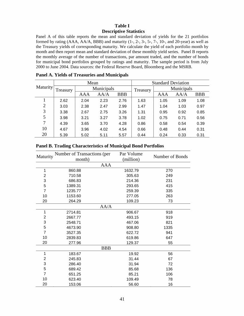
41

Table I Descriptive Statistics

Panel A of this table reports the mean and standard deviation of yields for the 21 portfolios formed by rating (AAA, AA/A, BBB) and maturity (1-, 2-, 3-, 5-, 7-, 10-, and 20-year) as well as the Treasury yields of corresponding maturity. We calculate the yield of each portfolio month by month and then report mean and standard deviation of these monthly yield series. Panel B reports the monthly average of the number of transactions, par amount traded, and the number of bonds for municipal bond portfolios grouped by ratings and maturity. The sample period is from July 2000 to June 2004. Data sources: the Federal Reserve Board, Bloomberg and the MSRB.

Panel A. Yields of Treasuries and Municipals

Mean Standard Deviation Municipals Municipals Maturity Treasury

AAA AA/A BBB Treasury

AAA AA/A BBB 1 2.62 2.04 2.23 2.76 1.63 1.05 1.09 1.08 2 3.03 2.38 2.47 2.99 1.47 1.04 1.03 0.97 3 3.38 2.67 2.75 3.26 1.31 0.95 0.92 0.85 5 3.98 3.21 3.27 3.78 1.02 0.75 0.71 0.56 7 4.39 3.65 3.70 4.28 0.86 0.58 0.54 0.39 10 4.67 3.96 4.02 4.54 0.66 0.48 0.44 0.31 20 5.39 5.02 5.11 5.57 0.44 0.24 0.33 0.31

Panel B. Trading Characteristics of Municipal Bond Portfolios

Maturity Number of Transactions (per month)

Par Volume (million) Number of Bonds

AAA 1 860.88 1632.79 270 2 710.58 305.63 249 3 686.83 214.36 231 5 1389.31 293.65 415 7 1235.77 259.39 335

10 1153.60 277.05 263 20 264.29 109.23 73

AA/A 1 2714.81 906.67 918 2 2667.77 493.15 919 3 2548.71 467.06 821 5 4673.90 908.80 1335 7 3527.35 622.72 941

10 2839.83 619.86 647 20 277.96 129.37 55

BBB 1 183.67 19.92 56 2 245.83 31.44 67 3 286.40 31.94 72 5 689.42 85.68 136 7 651.25 85.21 106

10 623.40 109.49 78 20 153.06 56.60 16

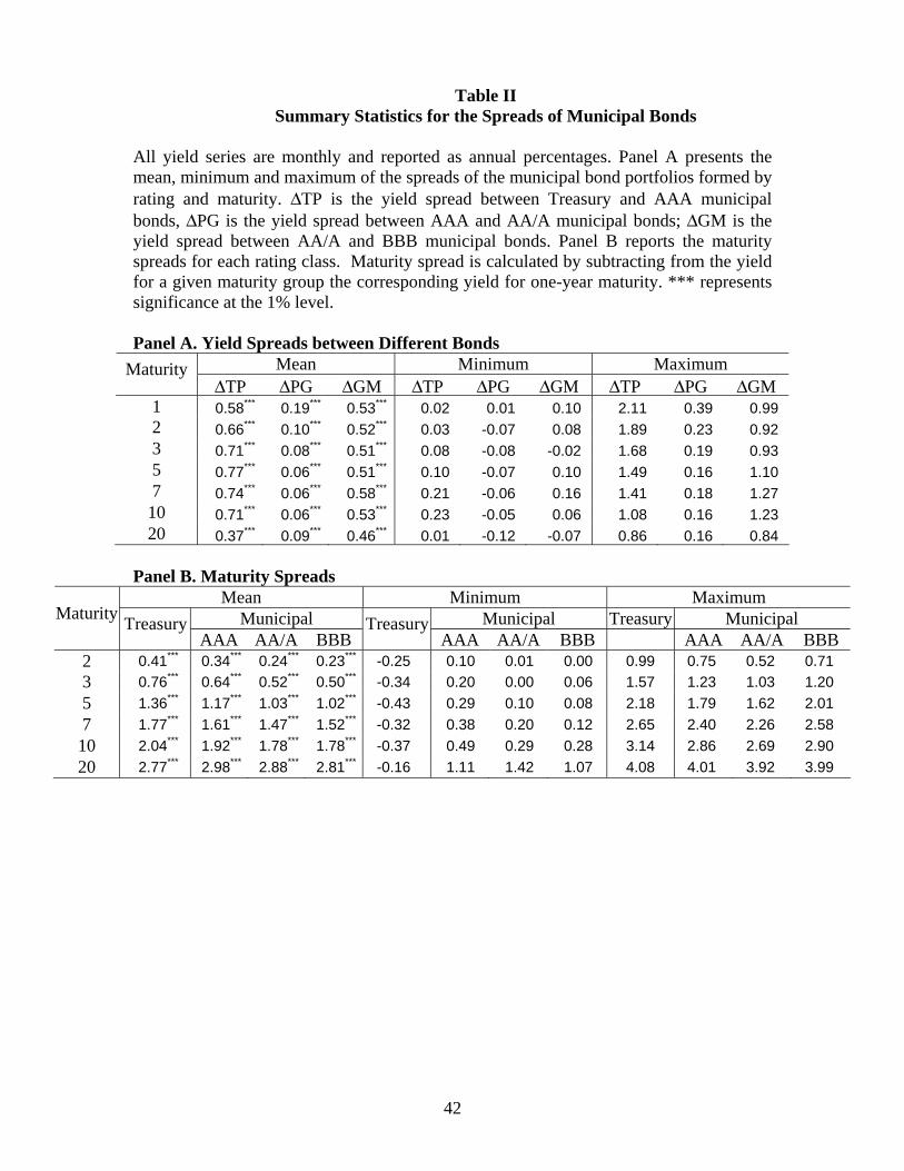
42

Table II Summary Statistics for the Spreads of Municipal Bonds

All yield series are monthly and reported as annual percentages. Panel A presents the mean, minimum and maximum of the spreads of the municipal bond portfolios formed by rating and maturity. ∆TP is the yield spread between Treasury and AAA municipal bonds, ∆PG is the yield spread between AAA and AA/A municipal bonds; ∆GM is the yield spread between AA/A and BBB municipal bonds. Panel B reports the maturity spreads for each rating class. Maturity spread is calculated by subtracting from the yield for a given maturity group the corresponding yield for one-year maturity. *** represents significance at the 1% level. Panel A. Yield Spreads between Different Bonds

Mean Minimum Maximum Maturity ∆TP ∆PG ∆GM ∆TP ∆PG ∆GM ∆TP ∆PG ∆GM

1 0.58*** 0.19*** 0.53*** 0.02 0.01 0.10 2.11 0.39 0.99 2 0.66*** 0.10*** 0.52*** 0.03 -0.07 0.08 1.89 0.23 0.92 3 0.71*** 0.08*** 0.51*** 0.08 -0.08 -0.02 1.68 0.19 0.93 5 0.77*** 0.06*** 0.51*** 0.10 -0.07 0.10 1.49 0.16 1.10 7 0.74*** 0.06*** 0.58*** 0.21 -0.06 0.16 1.41 0.18 1.27 10 0.71*** 0.06*** 0.53*** 0.23 -0.05 0.06 1.08 0.16 1.23 20 0.37*** 0.09*** 0.46*** 0.01 -0.12 -0.07 0.86 0.16 0.84

Panel B. Maturity Spreads

Mean Minimum Maximum Municipal Municipal Treasury Municipal Maturity Treasury

AAA AA/A BBB Treasury

AAA AA/A BBB AAA AA/A BBB 2 0.41*** 0.34*** 0.24*** 0.23*** -0.25 0.10 0.01 0.00 0.99 0.75 0.52 0.71 3 0.76*** 0.64*** 0.52*** 0.50*** -0.34 0.20 0.00 0.06 1.57 1.23 1.03 1.20 5 1.36*** 1.17*** 1.03*** 1.02*** -0.43 0.29 0.10 0.08 2.18 1.79 1.62 2.01 7 1.77*** 1.61*** 1.47*** 1.52*** -0.32 0.38 0.20 0.12 2.65 2.40 2.26 2.58 10 2.04*** 1.92*** 1.78*** 1.78*** -0.37 0.49 0.29 0.28 3.14 2.86 2.69 2.90 20 2.77*** 2.98*** 2.88*** 2.81*** -0.16 1.11 1.42 1.07 4.08 4.01 3.92 3.99

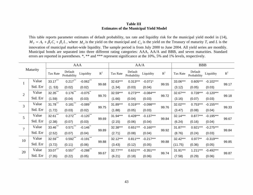
43

Table III

Estimates of the Municipal Yield Model

This table reports parameter estimates of default probability, tax rate and liquidity risk for the municipal yield model in (14), LCM LtTTT ββΛ ++= , where TM is the yield on the municipal and TC is the yield on the Treasury of maturity T, and L is the

innovation of municipal market-wide liquidity. The sample period is from July 2000 to June 2004. All yield series are monthly. Municipal bonds are separated into three different rating categories: AAA, AA/A and BBB, and seven maturities. Standard errors are reported in parentheses. *, ** and *** represent significance at the 10%, 5% and 1% levels, respectively.

AAA AA/A BBB

Maturity Tax Rate Default

Probability Liquidity R2 Tax Rate Default Probability Liquidity R2 Tax Rate Default

Probability Liquidity R2

Value 33.17*** 0.217*** -0.062*** 32.63*** 0.313*** -0.071* 33.06*** 0.605*** -0.102***1 Std. Err (1. 53) (0.02) (0.02)

99.68 (1.34) (0.03) (0.04)

99.55 (3.12) (0.05) (0.03)

99.17

Value 32.35*** 0.176*** -0.075** 32.59*** 0.273*** -0.084*** 32.67*** 0.728*** -0.120***2 Std. Err (1.59) (0.04) (0.03)

99.70 (1.66) (0.04) (0.03)

99.72 (3.16) (0.07) (0.03)

99.18

Value 31.78*** 0.181*** -0.089** 31.89*** 0.319*** -0.098*** 32.02*** 0.753*** -0.155***3 Std. Err (1.72) (0.03) (0.02)

99.75 (1.88) (0.05) (0.03)

99.76 (3.47) (0.08) (0.04)

99.33

Value 32.61*** 0.272*** -0.120*** 31.94*** 0.428*** -0.137*** 32.14*** 0.877*** -0.195***5 Std. Err (2.38) (0.07) (0.03)

99.69 (2.15) (0.06) (0.04)

99.84 (6.24) (0.16) (0.04)

99.67

Value 33.46*** 0.571*** -0.146** 32.38*** 0.651*** -0.160*** 31.87*** 0.921*** -0.275***7 Std. Err (2.52) (0.07) (0.04)

99.89 (2.71) (0.08) (0.04)

99.92 (8.76) (0.24) (0.03)

99.84

Value 32.59*** 0.592*** -0.191*** 32.12*** 0.811*** -0.217*** 32.42*** 0.977** -0.319***10 Std. Err (3.72) (0.11) (0.06)

99.88 (3.43) (0.12) (0.05)

99.88 (11.75) (0.36) (0.05)

99.85

Value 33.07*** 0.557** -0.288*** 32.77*** 0.631*** -0.351*** 31.91*** 1.211*** -0.492***20 Std. Err (7.35) (0.22) (0.05)

99.67 (6.21) (0.18) (0.06)

99.74 (7.58) (0.29) (0.06)

99.87

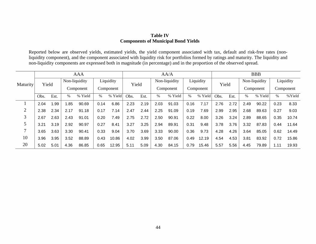
44

Table IV Components of Municipal Bond Yields

Reported below are observed yields, estimated yields, the yield component associated with tax, default and risk-free rates (non-liquidity component), and the component associated with liquidity risk for portfolios formed by ratings and maturity. The liquidity and non-liquidity components are expressed both in magnitude (in percentage) and in the proportion of the observed spread.

AAA AA/A BBB

Yield Non-liquidity

Component

Liquidity

Component Yield

Non-liquidity Component

Liquidity Component

Yield Non-liquidity Component

Liquidity Component

Maturity

Obs. Est. % % Yield % % Yield Obs. Est. % % Yield % % Yield Obs. Est. % % Yield % %Yield

1 2.04 1.99 1.85 90.69 0.14 6.86 2.23 2.19 2.03 91.03 0.16 7.17 2.76 2.72 2.49 90.22 0.23 8.33 2 2.38 2.34 2.17 91.18 0.17 7.14 2.47 2.44 2.25 91.09 0.19 7.69 2.99 2.95 2.68 89.63 0.27 9.03 3 2.67 2.63 2.43 91.01 0.20 7.49 2.75 2.72 2.50 90.91 0.22 8.00 3.26 3.24 2.89 88.65 0.35 10.74 5 3.21 3.19 2.92 90.97 0.27 8.41 3.27 3.25 2.94 89.91 0.31 9.48 3.78 3.76 3.32 87.83 0.44 11.64 7 3.65 3.63 3.30 90.41 0.33 9.04 3.70 3.69 3.33 90.00 0.36 9.73 4.28 4.26 3.64 85.05 0.62 14.49 10 3.96 3.95 3.52 88.89 0.43 10.86 4.02 3.99 3.50 87.06 0.49 12.19 4.54 4.53 3.81 83.92 0.72 15.86 20 5.02 5.01 4.36 86.85 0.65 12.95 5.11 5.09 4.30 84.15 0.79 15.46 5.57 5.56 4.45 79.89 1.11 19.93

45

Table V Likelihood Ratio Tests

This table reports the likelihood ratio test statistics under the restriction that the effect of liquidity risk is equal to zero (i.e., Lβ = 0) in the nonlinear municipal yield model in (14). The test statistics follow an F distribution with (1, n-3) degrees of freedom. The critical F value is 4.0 at the five percent level.

Maturity AAA Bonds AA/A Bonds BBB Bonds

F (1,n-3) F (1,n-3) F (1,n-3) 1 4.18 16.00 27.37

2 15.33 13.42 7.45

3 11.50 12.55 4.74

5 7.67 6.57 4.26

7 4.60 4.38 4.54

10 5.31 5.34 7.45

20 5.31 4.26 13.89

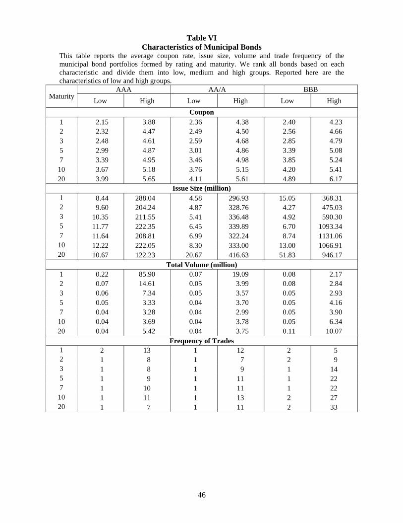
46

Table VI Characteristics of Municipal Bonds

This table reports the average coupon rate, issue size, volume and trade frequency of the municipal bond portfolios formed by rating and maturity. We rank all bonds based on each characteristic and divide them into low, medium and high groups. Reported here are the characteristics of low and high groups.

AAA AA/A BBB Maturity Low High Low High Low High

Coupon 1 2.15 3.88 2.36 4.38 2.40 4.23 2 2.32 4.47 2.49 4.50 2.56 4.66 3 2.48 4.61 2.59 4.68 2.85 4.79 5 2.99 4.87 3.01 4.86 3.39 5.08 7 3.39 4.95 3.46 4.98 3.85 5.24

10 3.67 5.18 3.76 5.15 4.20 5.41 20 3.99 5.65 4.11 5.61 4.89 6.17

Issue Size (million) 1 8.44 288.04 4.58 296.93 15.05 368.31 2 9.60 204.24 4.87 328.76 4.27 475.03 3 10.35 211.55 5.41 336.48 4.92 590.30 5 11.77 222.35 6.45 339.89 6.70 1093.34 7 11.64 208.81 6.99 322.24 8.74 1131.06

10 12.22 222.05 8.30 333.00 13.00 1066.91 20 10.67 122.23 20.67 416.63 51.83 946.17

Total Volume (million) 1 0.22 85.90 0.07 19.09 0.08 2.17 2 0.07 14.61 0.05 3.99 0.08 2.84 3 0.06 7.34 0.05 3.57 0.05 2.93 5 0.05 3.33 0.04 3.70 0.05 4.16 7 0.04 3.28 0.04 2.99 0.05 3.90

10 0.04 3.69 0.04 3.78 0.05 6.34 20 0.04 5.42 0.04 3.75 0.11 10.07

Frequency of Trades 1 2 13 1 12 2 5 2 1 8 1 7 2 9 3 1 8 1 9 1 14 5 1 9 1 11 1 22 7 1 10 1 11 1 22

10 1 11 1 13 2 27 20 1 7 1 11 2 33

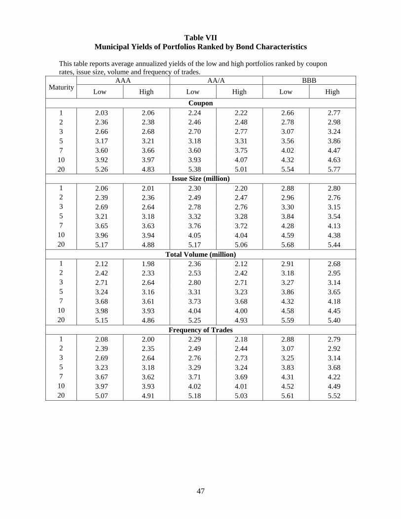
47

Table VII Municipal Yields of Portfolios Ranked by Bond Characteristics

This table reports average annualized yields of the low and high portfolios ranked by coupon rates, issue size, volume and frequency of trades.

AAA AA/A BBB Maturity Low High Low High Low High

Coupon 1 2.03 2.06 2.24 2.22 2.66 2.77 2 2.36 2.38 2.46 2.48 2.78 2.98 3 2.66 2.68 2.70 2.77 3.07 3.24 5 3.17 3.21 3.18 3.31 3.56 3.86 7 3.60 3.66 3.60 3.75 4.02 4.47

10 3.92 3.97 3.93 4.07 4.32 4.63 20 5.26 4.83 5.38 5.01 5.54 5.77

Issue Size (million) 1 2.06 2.01 2.30 2.20 2.88 2.80 2 2.39 2.36 2.49 2.47 2.96 2.76 3 2.69 2.64 2.78 2.76 3.30 3.15 5 3.21 3.18 3.32 3.28 3.84 3.54 7 3.65 3.63 3.76 3.72 4.28 4.13

10 3.96 3.94 4.05 4.04 4.59 4.38 20 5.17 4.88 5.17 5.06 5.68 5.44

Total Volume (million) 1 2.12 1.98 2.36 2.12 2.91 2.68 2 2.42 2.33 2.53 2.42 3.18 2.95 3 2.71 2.64 2.80 2.71 3.27 3.14 5 3.24 3.16 3.31 3.23 3.86 3.65 7 3.68 3.61 3.73 3.68 4.32 4.18

10 3.98 3.93 4.04 4.00 4.58 4.45 20 5.15 4.86 5.25 4.93 5.59 5.40

Frequency of Trades 1 2.08 2.00 2.29 2.18 2.88 2.79 2 2.39 2.35 2.49 2.44 3.07 2.92 3 2.69 2.64 2.76 2.73 3.25 3.14 5 3.23 3.18 3.29 3.24 3.83 3.68 7 3.67 3.62 3.71 3.69 4.31 4.22

10 3.97 3.93 4.02 4.01 4.52 4.49 20 5.07 4.91 5.18 5.03 5.61 5.52

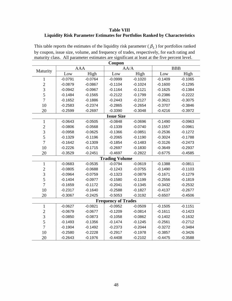
48

Table VIII Liquidity Risk Parameter Estimates for Portfolios Ranked by Characteristics

This table reports the estimates of the liquidity risk parameter ( Lβ ) for portfolios ranked by coupon, issue size, volume, and frequency of trades, respectively, for each rating and maturity class. All parameter estimates are significant at least at the five percent level.

Coupon AAA AA/A BBB Maturity Low High Low High Low High

1 -0.0791 -0.0764 -0.0999 -0.1020 -0.1409 -0.1065 2 -0.0879 -0.0867 -0.1104 -0.1024 -0.1600 -0.1295 3 -0.0942 -0.0967 -0.1164 -0.1121 -0.1625 -0.1384 5 -0.1484 -0.1565 -0.2122 -0.1799 -0.2386 -0.2222 7 -0.1652 -0.1886 -0.2443 -0.2127 -0.3621 -0.3075 10 -0.2583 -0.2374 -0.2865 -0.2654 -0.3707 -0.3846 20 -0.2599 -0.2697 -0.3390 -0.3048 -0.4216 -0.3972

Issue Size 1 -0.0643 -0.0505 -0.0848 -0.0696 -0.1490 -0.0963 2 -0.0806 -0.0568 -0.1339 -0.0740 -0.1557 -0.0961 3 -0.0958 -0.0625 -0.1366 -0.0851 -0.2536 -0.1272 5 -0.1329 -0.1196 -0.2065 -0.1190 -0.3024 -0.1788 7 -0.1642 -0.1309 -0.1854 -0.1483 -0.3126 -0.2473 10 -0.2226 -0.1715 -0.2697 -0.1830 -0.3649 -0.2937 20 -0.3529 -0.2451 -0.4697 -0.2822 -0.6775 -0.4585

Trading Volume 1 -0.0683 -0.0535 -0.0794 -0.0619 -0.1388 -0.0811 2 -0.0805 -0.0688 -0.1243 -0.0755 -0.1490 -0.1103 3 -0.0964 -0.0759 -0.1323 -0.0879 -0.1671 -0.1279 5 -0.1404 -0.0977 -0.1580 -0.1199 -0.2556 -0.1819 7 -0.1659 -0.1172 -0.2041 -0.1345 -0.3432 -0.2532 10 -0.2317 -0.1640 -0.2588 -0.1827 -0.4137 -0.2677 20 -0.3067 -0.2425 -0.5053 -0.3192 -0.6507 -0.4506

Frequency of Trades 1 -0.0627 -0.0821 -0.0952 -0.0509 -0.1505 -0.1151 2 -0.0679 -0.0677 -0.1209 -0.0814 -0.1611 -0.1423 3 -0.0850 -0.0873 -0.1058 -0.0862 -0.1402 -0.1632 5 -0.1493 -0.1356 -0.1474 -0.1245 -0.2561 -0.2712 7 -0.1904 -0.1492 -0.2373 -0.2044 -0.3272 -0.3484 10 -0.2580 -0.2228 -0.2917 -0.1978 -0.3857 -0.3426 20 -0.2643 -0.1976 -0.4408 -0.2102 -0.4475 -0.3588

49

Table IX Estimates of Liquidity Spreads for Different Characteristic Portfolios

This table reports the estimates of liquidity risk premium in magnitude (%) and proportion of the observed spread (% yield) for each high and low portfolio ranked by coupon rates, issue size, volume, and frequency of trades, respectively, for each rating and maturity class.

Coupon AAA AA/A BBB

Low High Low High Low High Maturity % % Yield % % Yield % % Yield % % Yield % % Yield % % Yield

1 0.18 8.87 0.17 8.25 0.23 10.27 0.23 10.36 0.32 12.03 0.24 8.66 2 0.20 8.47 0.20 8.40 0.25 10.16 0.23 9.27 0.36 12.95 0.29 9.73 3 0.21 7.89 0.22 8.21 0.26 9.63 0.25 9.03 0.37 12.05 0.31 9.57 5 0.34 10.73 0.35 10.90 0.48 15.09 0.41 12.39 0.54 15.17 0.50 12.95 7 0.37 10.28 0.43 11.75 0.55 15.28 0.48 12.80 0.82 20.40 0.69 15.44 10 0.58 14.80 0.54 13.60 0.65 16.54 0.60 14.74 0.84 19.44 0.87 18.79 20 0.59 11.22 0.61 12.63 0.77 14.31 0.69 13.77 0.95 17.15 0.90 15.60

Mean 0.35 10.32 0.36 10.54 0.46 13.04 0.41 11.77 0.60 15.60 0.54 12.96 Issue Size

1 0.15 7.28 0.11 5.47 0.19 8.26 0.16 7.27 0.34 11.81 0.22 7.86 2 0.18 7.53 0.13 5.51 0.30 12.05 0.17 6.88 0.35 11.82 0.22 7.97 3 0.22 8.18 0.14 5.30 0.31 11.15 0.19 6.88 0.57 17.27 0.29 9.21 5 0.30 9.35 0.27 8.49 0.47 14.16 0.27 8.23 0.68 17.71 0.40 11.30 7 0.37 10.14 0.30 8.26 0.42 11.17 0.34 9.14 0.71 16.59 0.56 13.56 10 0.50 12.63 0.39 9.90 0.61 15.06 0.41 10.15 0.82 17.86 0.66 15.07 20 0.80 15.47 0.55 11.27 1.06 20.50 0.64 12.65 1.53 26.94 1.04 19.12

Mean 0.36 10.08 0.27 7.74 0.48 13.19 0.31 8.74 0.71 17.14 0.48 12.01 Trading Volume

1 0.15 7.08 0.12 6.06 0.18 7.63 0.14 6.60 0.31 10.65 0.18 6.72 2 0.18 7.44 0.16 6.87 0.28 11.07 0.17 7.02 0.34 10.69 0.25 8.47 3 0.22 8.12 0.17 6.44 0.30 10.71 0.20 7.38 0.38 11.62 0.29 9.24 5 0.32 9.88 0.22 6.96 0.36 10.88 0.27 8.36 0.58 15.03 0.41 11.23 7 0.37 10.05 0.26 7.20 0.46 12.33 0.30 8.15 0.78 18.06 0.57 13.64 10 0.52 13.07 0.37 9.41 0.58 14.36 0.41 10.25 0.93 20.31 0.61 13.71 20 0.69 13.40 0.55 11.32 1.14 21.71 0.72 14.60 1.47 26.30 1.02 18.89

Mean 0.35 9.86 0.26 7.75 0.47 12.67 0.32 8.91 0.68 16.09 0.48 11.70 Frequency of Trades

1 0.14 6.73 0.19 9.50 0.22 9.61 0.12 5.50 0.34 11.81 0.26 9.32 2 0.15 6.28 0.15 6.38 0.27 10.84 0.18 7.38 0.36 11.73 0.32 10.96 3 0.19 7.06 0.20 7.58 0.24 8.70 0.19 6.96 0.32 9.85 0.37 11.78 5 0.34 10.53 0.31 9.75 0.33 10.03 0.28 8.64 0.58 15.14 0.61 16.58 7 0.43 11.72 0.34 9.39 0.54 14.56 0.46 12.47 0.74 17.17 0.79 18.72 10 0.58 14.61 0.50 12.72 0.66 16.42 0.45 11.22 0.87 19.25 0.77 17.15 20 0.60 11.83 0.45 9.16 1.00 19.31 0.48 9.54 1.01 18.00 0.81 14.67

Mean 0.35 9.82 0.31 9.21 0.47 12.78 0.31 8.82 0.60 14.71 0.56 14.17

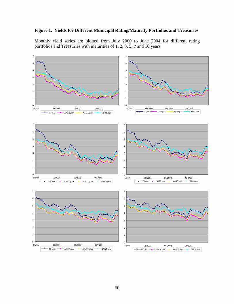
50

Figure 1. Yields for Different Municipal Rating/Maturity Portfolios and Treasuries Monthly yield series are plotted from July 2000 to June 2004 for different rating portfolios and Treasuries with maturities of 1, 2, 3, 5, 7 and 10 years.

0

1

2

3

4

5

6

7

Month 06/2001 06/2002 06/2003

T1year AAA1year AA/A1year BBB1year

0

1

2

3

4

5

6

7

Month 06/2001 06/2002 06/2003T2 year AAA2 year AA/A2 year BBB2 year

0

1

2

3

4

5

6

7

Month 06/2001 06/2002 06/2003

T3 year AAA3 year AA/A3 year BBB3 year

0

1

2

3

4

5

6

7

Month 06/2001 06/2002 06/2003T5 year AAA5 year AA/A5 year BBB5 year

0

1

2

3

4

5

6

7

Month 06/2001 06/2002 06/2003

T7 year AAA7 year AA/A7 year BBB7 year

0

1

2

3

4

5

6

7

Month 06/2001 06/2002 06/2003

T10 year AAA10 year AA/A10 year BBB10 year

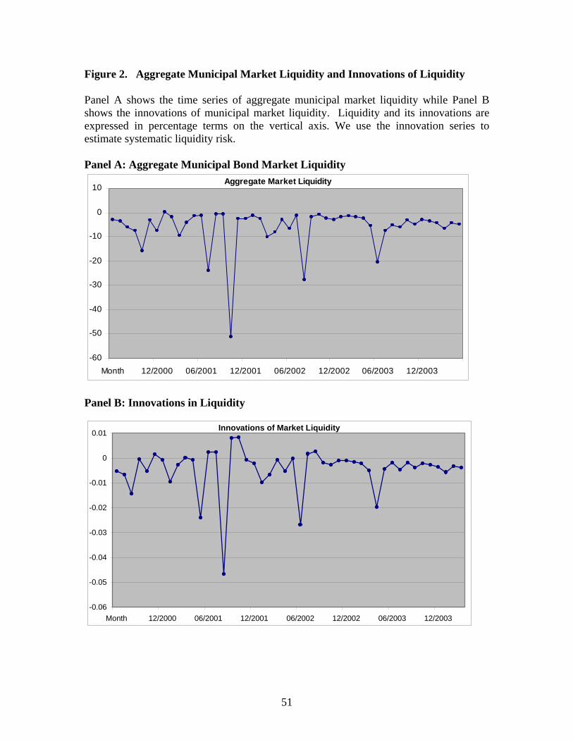
51

Figure 2. Aggregate Municipal Market Liquidity and Innovations of Liquidity Panel A shows the time series of aggregate municipal market liquidity while Panel B shows the innovations of municipal market liquidity. Liquidity and its innovations are expressed in percentage terms on the vertical axis. We use the innovation series to estimate systematic liquidity risk. Panel A: Aggregate Municipal Bond Market Liquidity

Aggregate Market Liquidity

-60

-50

-40

-30

-20

-10

0

10

Month 12/2000 06/2001 12/2001 06/2002 12/2002 06/2003 12/2003

Panel B: Innovations in Liquidity

Innovations of Market Liquidity

-0.06

-0.05

-0.04

-0.03

-0.02

-0.01

0

0.01

Month 12/2000 06/2001 12/2001 06/2002 12/2002 06/2003 12/2003