Liquidity Creation as Volatility Risk
45
Liquidity Creation as Volatility Risk Itamar Drechsler, Alan Moreira, Alexi Savov * April 2018 Abstract We show, both theoretically and empirically, that liquidity creation induces nega- tive exposure to volatility risk. Intuitively, liquidity creation involves taking positions that can be exploited by privately informed investors. These investors’ ability to pre- dict future price changes makes their payoff resemble a straddle (a combination of a call and a put). By taking the other side, liquidity providers are implicitly short a straddle, suffering losses when volatility spikes. Empirically, we show that short-term reversal strategies, which mimic liquidity creation by buying stocks that go down and selling stocks that go up, have a large negative exposure to volatility shocks. This ex- posure, together with the large premium investors demand for bearing volatility risk, explains why liquidity creation earns a premium, why this premium is strongly in- creasing in volatility, and why times of high volatility like the 2008 financial crisis trigger a contraction in liquidity. Taken together, these results provide a new, asset- pricing view of the risks and rewards to financial intermediation. JEL Codes: Keywords: Liquidity, volatility, reversals, VIX, variance premium * Drechsler and Savov are at New York University and NBER, [email protected] and [email protected]. Moreira is at University of Rochester, [email protected]. We thank Markus Brunnermeier (discussant) and participants at the NBER Asset Pricing Workshop for their com- ments. We thank Liz Casano for excellent research assistance. Suggestions and comments are welcome.
Transcript of Liquidity Creation as Volatility Risk

Liquidity Creation as Volatility Risk
Itamar Drechsler, Alan Moreira, Alexi Savov∗
April 2018
Abstract
We show, both theoretically and empirically, that liquidity creation induces nega-tive exposure to volatility risk. Intuitively, liquidity creation involves taking positionsthat can be exploited by privately informed investors. These investors’ ability to pre-dict future price changes makes their payoff resemble a straddle (a combination ofa call and a put). By taking the other side, liquidity providers are implicitly short astraddle, suffering losses when volatility spikes. Empirically, we show that short-termreversal strategies, which mimic liquidity creation by buying stocks that go down andselling stocks that go up, have a large negative exposure to volatility shocks. This ex-posure, together with the large premium investors demand for bearing volatility risk,explains why liquidity creation earns a premium, why this premium is strongly in-creasing in volatility, and why times of high volatility like the 2008 financial crisistrigger a contraction in liquidity. Taken together, these results provide a new, asset-pricing view of the risks and rewards to financial intermediation.
JEL Codes:Keywords: Liquidity, volatility, reversals, VIX, variance premium
∗Drechsler and Savov are at New York University and NBER, [email protected] [email protected]. Moreira is at University of Rochester, [email protected]. We thankMarkus Brunnermeier (discussant) and participants at the NBER Asset Pricing Workshop for their com-ments. We thank Liz Casano for excellent research assistance. Suggestions and comments are welcome.

We show, both theoretically and empirically, that liquidity creation—making assets
cheaper to trade than they otherwise would be—induces exposure to volatility risk. Given
the very large premium investors pay to avoid volatility risk (Carr and Wu, 2008), this ex-
plains why liquidity creation earns a premium (Krishnamurthy and Vissing-Jorgensen,
2015), why this premium is strongly increasing in volatility (Nagel, 2012), and why times
of high volatility like the 2008 financial crisis trigger a contraction in liquidity (Brunner-
meier, 2009). Taken together, these results provide a new, asset-pricing view of the risks
and rewards of financial intermediation.
Why does liquidity creation induce exposure to volatility risk? To create liquidity for
some investors in an asset, a liquidity provider takes positions that can be exploited by
other, privately informed investors (e.g. Kyle, 1985). These investors buy the asset if they
think it will rise in value and sell it if they think it will fall. Their ex post payoff therefore
resembles a straddle (a combination of a call and a put option). Like any straddle, this
payoff is high if volatility rises and low if it falls. By taking the other side, the liquidity
provider is implicitly short the straddle, earning a low payoff if volatility rises and a high
one if it falls. In other words, the liquidity provider is exposed to volatility risk.
The relation between liquidity creation and volatility risk is fundamental; it arises
directly from the presence of asymmetric information (a staple of the literature since Ak-
erlof, 1970). As a result, it applies widely across a variety of market structures. For in-
stance, one way financial institutions create liquidity is by issuing relatively safe securities
against risky assets (Gorton and Pennacchi, 1990). In doing so, they are betting against
private information possessed by those who originate the assets or in some other way
take a position against them (e.g. through derivatives). Consequently, when volatility
spikes and this private information becomes more valuable, financial institutions suffer
losses, as they did during the 2008 financial crisis.
Financial institutions and other investors also create liquidity by trading in secondary
markets such as those for stocks and bonds. We present a model to formalize how this
type of liquidity creation induces volatility risk and how this risk drives the liquidity
premium. We also use the model to motivate our empirical analysis.
The model builds on the framework of Kyle (1985), but with the added ingredient of
1

stochastic volatility. A liquidity provider observes order flow, which captures the liquid-
ity demand of informed and uninformed investors alike. She sets prices to break even on
average, earning profits against the uninformed to offset losses against the informed. To
do so, she has to predict the value of the informed investors’ private signal. This value
depends on the remaining volatility in the asset’s payoff. As a result, prices conditional
on order flow depend on expected volatility going forward. When expected volatility
is high, assets with negative order flow have lower prices and assets with positive order
flow have higher prices. When expected volatility is low, prices depend less on order flow.
If, however, volatility rises in the following period, the value of the informed investors’
information also rises. This earns them a higher expected profit than was priced in by the
liquidity provider who therefore incurs an expected loss. Thus, the liquidity provider has
a negative exposure to volatility shocks. The magnitude of this exposure depends on the
expected size of these shocks, i.e. on the volatility of volatility.
The model has many assets and liquidity providers are free to trade all of them. Yet
they cannot diversify away their volatility risk because volatility follows a factor struc-
ture across assets. As Herskovic et al. (2016) show, this assumption is strongly supported
in the data. Also strongly supported is that the factors that drive asset-level volatility are
highly correlated with aggregate volatility (e.g. Campbell et al., 2001; Bekaert, Hodrick
and Zhang, 2012). Hence, our model predicts that liquidity providers have negative ex-
posure to aggregate as well as asset-level volatility. The asset pricing literature shows that
aggregate volatility in particular carries a very large negative risk premium (Carr and Wu,
2008; Bollerslev, Tauchen and Zhou, 2009).1 Therefore, our model predicts that liquidity
providers should earn a positive premium for their negative exposure to volatility. This
liquidity premium arises purely as compensation for bearing volatility risk.
We test the predictions of our model using U.S. stock return data from 2001 to 2016
(covering the period after “decimalization,” when liquidity provision became competi-
tive; see Bessembinder, 2003). Each day, we sort stocks into deciles based on their return
(normalized by its rolling standard deviation) and quintiles based on their size (small
1Given the high correlation between asset-level and aggregate volatility, it is possible that the priced riskfactor is actually asset-level volatility and not aggregate volatility, or that the premium is for both, but thispossibility is rarely explored in the literature. Herskovic et al. (2016) is one exception.
2

stocks are known to be much less liquid). Within each size quintile, we construct long-
short portfolios that buy stocks in the low return deciles and sell stocks in the high return
deciles. These are known as short-term reversal portfolios in the literature (e.g. Lehmann,
1990). In our model, a large return reflects high order flow and hence high liquidity de-
mand.2 The reversal portfolio therefore mimics the position of the liquidity provider,
hence, as in Nagel (2012), we can use it to analyze the returns to liquidity creation.
Consistent with the model, and with the prior literature, our reversal portfolios earn
substantial returns that cannot be explained by exposure to market risk. Among large
stocks, which account for the bulk of the market by value, the reversal strategy across the
lowest and highest return deciles has an average return of 27 bps over a five day holding
period, or about 13.5% per year. The annual Sharpe ratio is 0.6.
Figure 1 plots the return of the large-stock reversal strategy averaged over a 60-day
forward-looking window against the level of VIX, a risk-neutral measure of the expected
volatility of the S&P 500 over the next 30 days. The figure shows that the reversal return
is strongly positively related to VIX (the raw correlation is 46%). In a regression, we
find that a one-point higher VIX leads to a 5.37 bps higher reversal return over the next
five days, which is large relative to the average return of the strategy. The R2 of this
regression is 2.18%, which is very high for daily data. These findings confirm the main
result of Nagel (2012) that VIX predicts reversal returns.3 They are also a prediction of
our model. A high level of VIX is associated not only with high expected volatility but
also with high volatility of volatility (and high aversion to volatility risk). In our model
this makes liquidity creation riskier and raises the price of liquidity.
The bottom panel of Figure 1 tests this mechanism by plotting a measure of the volatil-
ity risk of the reversal strategy. We compute it by running 60-day rolling window regres-
sions of the five-day large-stock reversal return on the daily VIX changes during the hold-
ing period. The figure plots the annualized standard deviation of the fitted value from
this regression, which captures the systematic volatility of the reversal strategy due to
2In practice, returns also reflect the release of public news, which makes them a noisy proxy. To partlyreduce this noise, we follow Collin-Dufresne and Daniel (2014) and remove earnings announcement days.
3Our methodology differs somewhat from Nagel (2012) in that we focus on large stocks and opt fordecile sorting instead of weighting by returns.
3
VIX changes, i.e. its volatility risk. The figure shows that the volatility risk of the reversal
strategy is substantial and that it covaries strongly with the level of VIX (the raw correla-
tion is 58%). This confirms the prediction that when VIX is high the reversal strategy is
exposed to more volatility risk, which is consistent with its higher premium.
To formally test if the reversal strategy is exposed to volatility risk, we regress its
return on changes in VIX. We find a strong negative beta coefficient: the five-day large-
stock reversal return drops by 64 bps if VIX rises by an average of one point per day
over the holding period, which is equivalent to 1.3 standard deviations. The beta is large
relative to the average return of the strategy (27 bps). It rises to 71 bps if we control for the
market return, and the results are similar for small stocks. Thus, the reversal strategies
have substantial negative exposure to volatility risk, a central prediction of the model.
The negative impact of VIX changes on the reversal strategy returns is highly persis-
tent. A one-point increase in VIX one day after portfolio formation induces a same-day
drop of 19-bps in the large-stock reversal strategy, which remains essentially unchanged
at 21 bps by the end of the holding period. This persistence is in line with our model
where an increase in expected volatility raises the value of private information about the
value of the asset. It goes against alternative models where a rise in VIX forces constrained
liquidity providers to offload their positions. In such a model the impact on prices would
be transitory.
The next step in our analysis is to test whether this volatility risk exposure can account
for the average returns of the reversal strategies. This prediction differentiates our the-
ory from others, which are based on the inventory risk of liquidity providers (Stoll, 1978;
Grossman and Miller, 1988; Gromb and Vayanos, 2002; Duffie, 2010). We note that inven-
tory risk is in principle fully diversifiable, hence it should not command any premium, let
alone one as large as the one we find in this recent sample. This tension is present in all
models of the liquidity premium based on inventory risk. In contrast, our model shows
that there is a tight relationship between liquidity creation and volatility risk, which is
nondiversifiable, and thus ties together their premiums.
Our first pricing test runs Fama-MacBeth regressions of the five-day reversal portfolio
returns on the daily market returns and VIX changes during the holding period. We find
4

that exposure to VIX changes is strongly priced and substantially reduces the pricing er-
rors of the portfolios. The pricing error of the largest quintile reversal strategy drops from
25 bps to −7 bps. The pricing errors of the next two quintiles are similarly driven down
(20 bps to 4 bps and 33 bps to 6 bps, respectively). Only the pricing errors of the two
smallest quintiles remain significant (these stocks account for just 0.4% of market value).
Hence, outside these very small stocks, our results show that the returns to liquidity pro-
vision are well priced by volatility risk exposures.
Our final test asks if volatility risk can price the reversal strategies with the same price
of risk that prevails in other markets. If so, it would suggest that the price of liquidity
creation reflects broad economic risks rather than institutional frictions.
The natural place to measure the price of volatility risk is in option markets. The
VIX index itself is based on the price of a basket of options whose payoff replicates the
realized variance of the S&P 500 over a 30-day period. Since this basket changes from day
to day as options near expiration, the change in VIX is not a valid return from which we
can estimate a price of risk. However, it is straight-forward to compute such a return by
simply holding the basket fixed from one day to the next. We do so using data on S&P 500
options and following the methodology of the Chicago Board Options Exchange (CBOE).
The resulting VIX return has a sample average of −1.54% per day.
Whereas VIX has a 30-day horizon, liquidity provision in equity markets typically
takes place on a shorter time scale. This is why we follow the literature and focus on
reversal returns out to five trading days. While it is not feasible to target such a short
horizon with index option data,4 we are able to move in that direction by calculating the
return associated with VIXN, the “near-term VIX”, which is one of the two cross sections
of options used by CBOE in the computation of VIX (the average horizon of VIXN is 22
days). We find that the VIXN return is −2.01% per day, which is larger even than the VIX
return.
We calculate a price of risk associated with exposure to VIX changes by dividing the
average VIX return by its loading on VIX changes. This gives a price of −22 bps, i.e.
4Options often behave erratically near expiration, hence the CBOE discards options with less than aweek to expiration from the computation of VIX.
5

an asset that rises by one percent when VIX rises by one point is predicted to have an
average return of −22 bps per day. We do the same for the VIXN return with respect to
VIXN changes and obtain a price of risk of −33 bps.
Using these prices of risk and the betas of the reversal portfolios, we calculate pre-
dicted returns and pricing errors.5 We find that these restricted pricing tests perform
similarly to the unrestricted Fama-MacBeth regressions, especially when we use the near-
term VIXN. Specifically, when we use VIX changes as the priced factor and the VIX re-
turn to obtain its price, the pricing error of the large-stock five-day reversal strategy drops
from 25 bps to 11 bps and remains marginally significant. On the other hand, when we
use VIXN changes as the priced factor and the VIXN return to obtain its price, this pric-
ing error drops to just 1 bp. Thus, near-term volatility risk prices the large-stock reversal
strategy almost perfectly. The pricing errors of the second and third largest quintiles also
become insignificant. Only the two smallest quintiles retain significant pricing errors,
similar to the Fama-MacBeth regressions. Overall, these results indicate that the returns
to liquidity creation reflect compensation for the risks of betting against volatility.
The rest of this paper is organized as follows. Section 1 reviews the literature, Section
2 presents the model, Section 3 introduces the data, Section 4 discusses the empirical
results, and Section 5 concludes.
1 Related literature
A large literature in asset pricing studies how liquidity is priced in financial markets.
Amihud and Mendelson (1986) and Brennan and Subrahmanyam (1996) show that illiq-
uid stocks have higher expected returns. Chordia, Roll and Subrahmanyam (2000) and
Hasbrouck and Seppi (2001) show that different measures of illiquidity comove strongly.
Amihud (2002) and Pástor and Stambaugh (2003) show that aggregate illiquidity is priced
both in the time series and cross section of stocks. Acharya and Pedersen (2005) provide
an equilibrium model that captures these facts. This literature has also shown that liq-
5This is analogous to including the VIX and VIXN returns as additional test assets and imposing therestriction that they be priced perfectly. This approach is also followed by Constantinides, Jackwerth andSavov (2013).
6

uidity is decreasing in volatility. Chordia, Sarkar and Subrahmanyam (2004) show that
increases in volatility are associated with a reduction in liquidity. Hameed, Kang and
Viswanathan (2010) show that liquidity provision strategies earn high returns following
stock market downturns. Nagel (2012) shows that expected returns to liquidity provision
in stocks are increasing in the level of VIX.
A second large literature in asset pricing studies how volatility is priced in financial
markets. Carr and Wu (2008) show that investors pay a large premium (the variance risk
premium) to hedge aggregate volatility risk. Todorov (2009) and Bollerslev and Todorov
(2011) extend these results to jump risk. Bollerslev, Tauchen and Zhou (2009) and Drech-
sler and Yaron (2010) show that the variance risk premium strongly predicts aggregate
stock returns. Manela and Moreira (2017) extend these results by over a century. Bao, Pan
and Wang (2011) and Longstaff et al. (2011) find similar results for bonds. Drechsler and
Yaron (2010), Drechsler (2013), and Dew-Becker et al. (2017) provide theories that explain
the behavior of the variance risk premium as driven by macroeconomic risk.
The contribution of our paper is to integrate the literatures on the pricing of liquidity
and volatility. First, we show theoretically that liquidity provision induces exposure to
volatility risk. Second, we confirm this prediction empirically and show that volatility
risk can explain the observed returns to liquidity provision strategies.
Our model is rooted in the theoretical literature on how asymmetric information im-
pacts asset prices and liquidity (e.g. Hellwig, 1980; Grossman and Stiglitz, 1980; Diamond
and Verrecchia, 1981; Kyle, 1985; Glosten and Milgrom, 1985). Specifically, we introduce
stochastic volatility in the framework of Kyle (1985).6 We show that informed traders
are effectively long a straddle because they can trade in the direction of subsequent price
changes. Liquidity providers, who take the other side, are therefore short a straddle. As
a result, they suffer losses when volatility comes in higher than expected. This expo-
sure cannot be diversified away because volatility is highly correlated across assets and
with market volatility. Our model shows how this leads to the emergence of a liquidity
6Collin-Dufresne and Fos (2016) solve a dynamic version of this framework with stochastic noise tradervolatility. While this feature does not create volatility risk exposure for the liquidity provider, our frame-works share the presence of long-lived private information, which contrasts with earlier papers like Admatiand Pfleiderer (1988) and Foster and Viswanathan (1990).
7

premium as compensation for volatility risk.
A more recent literature focuses on the role of financial frictions in generating fluc-
tuations in liquidity (e.g. Eisfeldt, 2004; He and Krishnamurthy, 2013; Brunnermeier and
Sannikov, 2014). Gromb and Vayanos (2002), Brunnermeier and Pedersen (2008), and
Adrian and Shin (2010) show how, when financial institutions are risk averse or subject
to a Value-at-Risk (VaR) constraint, a rise in volatility leads to a contraction in the supply
of liquidity. Moreira and Savov (2017) show how such a liquidity contraction impacts
asset prices and the macroeconomy. Our paper shows how these dynamics can arise as a
result of fluctuations in the variance risk premium. Of course, it is also possible that the
variance risk premium itself is a reflection of the scarcity of liquidity, particularly at the
short end. We return to this intriguing possibility at the end of the paper.
2 Model
We present a model in the tradition of Kyle (1985) that shows why liquidity provision
is fundamentally exposed to aggregate volatility risk and thus inherits its substantial,
negative price of risk. The model makes several further predictions and guides the con-
struction and implementation of our empirical tests.
There are three time periods, 0, 1, and an in-between period t ∈ (0, 1), and N assets
that are traded at time 0. There are three types of market participants: insiders, liquidity
demanders, and liquidity providers. For each asset there is a single insider, a unit mass
of liquidity demanders, and a competitive fringe of liquidity providers.
Each asset i has a single payoff pi,1 that is realized at time 1 and is given by:
pi,1 = vi + σi,1 vi, (1)
where vi is a constant and vi ∼ N (0, 1) is an idiosyncratic shock that is uncorrelated
across assets and is scaled by the volatility σi,1. Thus, σi,1 represents asset i’s idiosyncratic
volatility. The value of vi is known by all investors prior to time 0 and is the price of the
asset before any trading takes place. At time 0 insiders learn the value of vi, whereas its
8

value remains unknown to the other market participants. Trading then takes place.
All market participants share the same information and expectations about the ran-
dom variable σi,1, which is uncertain until time 1. The realization of σi,1 is driven by both
a market (i.e., systematic) volatility factor σm that is common to all N assets’ idiosyncratic
volatilities, and an asset-specific component εσi :
σi,1 = kiσm,1 + εσi . (2)
The parameter ki gives the loading of asset i’s idiosyncratic volatility on the market
volatility factor σm,1. We assume ki > 0 to capture the observed strong comovement
of idiosyncratic and market volatilities.
At the intermediate time t ∈ (0, 1), news arrives about volatilities that changes market
participants’ expectations of the value of σi,1. To focus on the impact of this volatility
news, we assume that only liquidity providers trade at time t, so that changes in prices at
this time are due only to updates in volatility expectations.
The single insider in each asset maximizes the value of profits under the economy’s
pricing kernel:7
y∗i = arg maxyi
EQ0 [yi (pi,1 − pi,0) | vi] , (3)
where EQ0 denotes expectation at time-0 under the risk-neutral probabilities implied by
the pricing kernel, yi is the insider’s share position in asset i, and pi,0 is the time-0 price
of the asset. Liquidity traders demand for shares of asset i is given by zi ∼ N(0, σ2
zi
),
which we assume is uncorrelated across assets. Finally, there is the unit mass of liquidity
providers. We assume liquidity providers are integrated with the rest of the market (no
segmentation), and thus also price payouts according to the economy’s pricing kernel.
As in Kyle (1985), liquidity providers cannot distinguish between the trades of in-
siders and liquidity traders and only observe their net order flow, Xi = zi + y∗i . Since
7The assumption of a single insider is inessential. We could instead model a mass of competitive insiderswho are risk-averse. The essential requirement is that some consideration limits the intensity of insiders’trading, so that their trading does not fully reveal their private information.
9

liquidity providers are competitive, they set the time-t price pi,t so that they break even
in expectation:
pi,t = EQt [pi,1 | Xi] . (4)
As in Kyle (1985), we conjecture (and later verify) that the insider’s demand is given by
y∗i = φ(
EQ0 [pi,1 | vi]− pi
)= φ
(vi + EQ
0 [σi,1] vi − pi
), (5)
where φ and pi are determined in equilibrium. By Bayes’ rule, the price at time t ∈ [0, 1)
is
pi,t = vi + EQt [σi,1] EQ
t [vi | Xi] = vi + EQt [σi,1] λXi, (6)
where λ =cov0 (vi, Xi)
var0(Xi)=
φEQ0 [σi,1]
φ2(EQ0 [σi,1])2 + σ2
zi
. (7)
The solution for λ is based only on time-0 information because the insider’s demand y∗i is
determined at time 0 and there is no additional information about vi in the time-t volatility
news. Substituting the price schedule (6) into the insider’s problem and simplifying gives:
y∗i = arg maxyi
EQ0
[yi
(EQ
0 [σi,1]vi − λEQ0 [σi,1](zi + yi)
) ∣∣∣ vi
](8)
= arg maxyi
yiEQ0 [σi,1]vi − y2
i λEQ0 [σi,1] (9)
=1
2λvi. (10)
Setting this expression equal to (5) and solving the resulting equation jointly with (7) gives
the values of λ, φ, and pi and confirms the conjecture (5) for y∗i . We obtain the following.
Proposition 1. φ, pi, and λ are given by
φ =σzi
EQ0 [σi,1]
, pi = vi, λ =1
2σzi
, (11)
10

and asset i’s price at time 0 ≤ t < 1 is
pi,t = vi +Xi
2σzi
EQt [σi,1]. (12)
Thus, the time-0 price is pushed in the direction of the net order flow Xi. This is intu-
itive since liquidity providers absorb this order flow by taking the opposite position,−Xi.
The sensitivity of the price to the order flow imbalance is inversely related to the expected
amount of uninformed liquidity trading, σzi , and proportional to expected volatility. A
higher expected volatility makes insiders’ information more powerful and thus increases
adverse selection, making the price more sensitive to imbalances in order flow.
Unfortunately, neither the sign nor magnitude of Xi are directly observable in the
data. While volume is observable, it is unsigned and represents only the gross quantity
of trading, whereas Xi is a net quantity. The relationship between net and gross can be
complicated and unstable across different assets and markets, depending on the number
of individual liquidity traders and the amount of netting that occurs within this group.
Fortunately, equation (12) shows that the change in the asset’s price at time 0 contains
information about the sign and magnitude of liquidity providers’ exposure to the asset’s
volatility. Let ∆pi,0 = (pi,0 − vi) denote asset i’s time-0 price change. We have the follow-
ing.
Lemma 1. The exposure of liquidity providers to asset i’s volatility, −Xi/σzi , is proportional to,
and has the opposite sign of, its time-0 price change:
−Xi
σzi
= −∆pi,02
EQ0 [σi,1]
(13)
Thus, liquidity providers hold a portfolio of reversals: they take larger long (short) exposures in
assets that have larger time-0 price decreases (increases).
Together, equations (12) and (13) show that assets’ time-0 price changes give their
exposures to volatility news. As the following proposition shows, liquidity providers are
negatively exposed to increases in volatility on all of their positions, both long and short.
When volatilities increase, both legs of the reversals go against the liquidity providers–
11

long positions decline while short positions advance. Let ∆pi,t = pi,t − pi,0 denote the
time-t price change of asset i. We have the following:
Proposition 2. The change in the price of asset i at time t is given by
∆pi,t =Xi
2σzi
(EQt [σi,1]− EQ
0 [σi,1]). (14)
and hence the beta of liquidity providers’ holdings of asset i (−Xi∆pi) to shocks to market volatility
(EQt [σm,1]− EQ
0 [σm,1]) is
βi,σm =−Xi∆pi,t
EQt [σi,1]− EQ
0 [σi,1]ki = −
X2i
2σzi
ki < 0. (15)
Thus, all of the liquidity provider’s positions, long and short, have negative betas to changes in
market volatility. When market volatility increases, the reversal portfolio loses on both sides–long
positions decline while short positions advance.
Therefore, the liquidity provider is negatively exposed to systematic, undiversifiable
market volatility risk. This is surprising because assets’ payoffs in the model are purely
idiosyncratic in nature, and have no correlation with the market return. Moreover, even
if there were market risks, liquidity providers hold zero-investment portfolios that are
neither net long nor short. Nevertheless, they have inescapably negative market volatility
betas. The explanation is that, even though assets’ cash flows are purely idiosyncratic,
there is commonality in their expected volatilities. It is this commonality in their second
moments that exposes the liquidity provider to an undiversifiable risk in the portfolio’s
first moment. This is important in practice, since empirically there is a very high degree
of commonality in volatilities, both idiosyncratic and systematic, across all assets.
A large literature in volatility and option pricing documents that market volatility
risk commands a very substantial and negative price of risk. Formally, this means that
EP0 [σm,1] < EQ
0 [σm,1], i.e., risk-adjusted (Q-measure) volatility expectations are substan-
tially higher than objective expectations, so that selling insurance against market volatil-
ity risk earns a large price premium. Since the reversal portfolio has a large negative beta
to this risk, the liquidity provider demands a large risk premium to bear it.
12
Proposition 3. The expected payoff on the liquidity provider’s portfolio from time 0 to time 1 is:
EP0
[N
∑i=1−Xi∆pi,1
]=
(N
∑i=1
βi,m
)(EP
0 [σm,1]− EQ0 [σm,1]
)> 0. (16)
Hence, the return to liquidity provision reflects the large volatility risk exposure of
the reversal portfolios, as captured by their market volatility betas.
For testing the model, it will be useful to create a cross-section of reversal portfolios
with differing exposures to market volatility risk. Equations (13) and (14) show this can
be done by forming a cross-section of reversal portfolios based on the magnitude of as-
sets’ time-0 price changes (returns). Within each reversal portfolio, one can approximate
the liquidity providers’ position (Xi) in each asset by weighting it by a proxy for σzi . Al-
though σzi is not directly observable, we can proxy for it using the asset’s volume, which
is proportional to σzi . Thus, the model predicts that we can obtain a cross-section of expo-
sures to market volatility risk by sorting assets into volume-weighted reversal portfolios
according to their time-0 returns.
3 Data and summary statistics
Stock screens: We construct reversal portfolios using data from CRSP. We exclude stocks
with missing market capitalization or trading volume, and stocks with prices below $1
(penny stocks). Following Collin-Dufresne and Daniel (2014), we also exclude stocks that
are within one day of an earnings announcement as recorded in COMPUSTAT. Earnings
announcements are overwhelmingly public information-driven (as opposed to liquidity-
driven) events, which confounds measurement of the returns to liquidity provision.8
Sample selection: The sample is daily from April 9, 2001 to December 31, 2016, which
covers 3,958 trading days. The starting date corresponds to “decimalization,” the transi-
tion from fractional to decimal pricing on the New York Stock Exchange and NASDAQ.
8Consistent with this view, the literature on post-earnings announcement drift shows that earnings an-nouncements are associated with return continuation rather than reversal (e.g. Bernard and Thomas, 1989).Interestingly, Sadka (2006) finds that this continuation is partly explained by liquidity risk, but does notexplore a connection to volatility risk.
13
As shown by Bessembinder (2003), decimalization saw a large decrease in effective trad-
ing costs, consistent with increased competition among liquidity providers. This implies
that the returns to liquidity provision prior to decimalization reflect monopolistic rents.
Portfolio formation: Each day, we double-sort stocks independently into quintiles by
market capitalization and deciles by normalized return. The sort by market capitalization
is motivated by the fact that return reversals decrease with size (Avramov, Chordia and
Goyal, 2006). The normalized return is computed as the z-score of each stock’s log return
relative to its distribution over the past 60 trading days (i.e. by subtracting the mean
and dividing by the standard deviation). The normalization ensures that the outer decile
portfolios are not dominated by stocks with the highest volatility.
The sort by normalized return captures variation in liquidity demand. In the model,
liquidity demand is given by the order flow variable Xi. Since prices are linear in order
flow, price changes (returns) give us a proxy for liquidity demand. Prices can change
for non-liquidity reasons such as the release of public news. This makes them a noisy
proxy for liquidity demand (this is why we remove earnings announcement days). The
identification assumption we are making is that this noise is uncorrelated with exposure
to volatility risk.
We weight stocks within each double-sorted portfolio by their dollar volume on the
sorting day. This mimics the economic exposure of liquidity providers, helping to capture
the risks that they face. Dollar volume is computed as trading volume times lagged price.
Lagging the price simply ensures that we are not weighting by the day’s return a second
time after sorting on it.
Following Nagel (2012), we hold each portfolio for one to five trading days. This
captures the returns to low-frequency liquidity provision. Whereas liquidity provision
in recent years has been dominated by high-frequency trading, low-frequency liquidity
provision remains important as long as imbalances between ultimate buyers and sellers
persist for more than one day. The presence of a reversal premium suggests that they
do. Our results show that the reversal premium has not declined with the rise of high-
frequency trading, suggesting that low-frequency liquidity provision remains scarce.
Aggregate factors: We use the excess CRSP value-weighted market return as the market
14
risk factor. We compute excess returns by subtracting the risk-free rate (the return on the
1-month T-Bill from CRSP).
We obtain the VIX index from the CBOE.
We measure aggregate idiosyncratic volatility, IVOL, as the value-weighted average
squared abnormal return across stocks. Abnormal returns are calculated using a market
model. IVOL is annualized to give it the same units as VIX.
The VIX return: We use S&P 500 options data from OptionMetrics to calculate the
VIX return (the data ends on April 29, 2016). The VIX index is a model-free measure of
the implied volatility of the S&P 500 index (as proposed by Britten-Jones and Neuberger,
2000). Specifically, the squared VIX is the price of a basket of options whose payoff is
the realized variance of the S&P 500 over the next 30 days. Because this basket changes
from day to day, the change in the squared VIX itself is not a valid return. However, the
percentage change in the price of a basket of options used to construct VIX on a given day
is a valid return. We refer to it as the VIX return.
To construct the VIX return, we first replicate the VIX itself by following the method-
ology provided by the CBOE.9 The replication is very accurate: our replicated VIX has a
99.83% correlation with the official VIX. The VIX return is the percentage change in the
price of the basket of options used to construct our replicated VIX.
To maintain its constant target maturity of 30 days, the VIX is computed from a
weighted average of the prices of two baskets of options, one with maturity less than
30 days (known as the near-term VIX) and one with maturity greater than 30 days (the
far-term VIX). The CBOE publishes these under the tickers VIXN and VIXF, respectively.
We construct their returns from the prices of the baskets that replicate them. The VIX
return is simply the weighted average of the VIXN and VIXF returns, with the weights
set to achieve an average maturity of 30 days.
9See the CBOE white paper at https://www.cboe.com/micro/vix/vixwhite.pdf. The current methodol-ogy uses SPX weekly options as well as the traditional monthly ones. It was first implemented on October6, 2014. Prior to this date, only the traditional monthly options were used.
15

3.1 Summary statistics
Table 1 presents summary statistics for the reversal portfolios. We focus on long-short
strategies across return deciles, e.g. 1–10 (labeled “Lo–Hi”), 2–9, 3–8, 4–7, and 5–6. These
are the return reversal strategies. The Lo–Hi strategy is based on the outermost return
deciles and hence carries the strongest reversal signal.
From the top panel of Table 1, there are about one hundred stocks on each side (long
and short) of each portfolio. The counts are slightly higher in the outer deciles for small
stocks and slightly lower for large stocks. The reason is that small stocks have return
distributions with fatter tails, which makes them more likely to have extreme returns
even after normalizing by their volatility.
The second panel of Table 1 reports market capitalizations. The typical stock in the
largest quintile is worth $50 billion, three orders of magnitude larger than the smallest
quintile and two orders larger than the middle quintile. The largest stocks account for
96.4% of the total value of all the portfolios, making them the by far the most important
quintile in economic terms (the smallest stocks account for less than 0.1%).
The third panel of Table 1 shows the sorting-day returns (without normalizing). Since
small stocks are more volatile than large stocks, their sorting-day returns are larger in
magnitude. For instance, the sorting-day return of the Lo–Hi strategy for the smallest
stocks is −24.36%, whereas for the largest stocks it is −7.45%.
The fourth panel of Table 1 looks at share turnover. It shows that the Lo–Hi strategy
has double the turnover of the middle decile strategies. This higher turnover, together
with the large sorting-day return and subsequent reversal, indicates that these stocks ex-
perience an outward shift in investors’ demand for liquidity. Liquidity providers absorb
this demand shift, allowing for higher turnover, but charge for it by allowing prices to
overshoot so they can revert later.
Finally, the bottom panel of Table 1 shows the illiquidity measure from Amihud
(2002), i.e. the absolute value of the return divided by dollar volume (multiplied by 106
for readability).10 As expected, illiquidity is strongly decreasing in size: the largest stocks
10Since we want to measure illiquidity on the sorting day, we do not average the measure for each stockover time as is customary. Instead, we average it across stocks within each portfolio and then over time for
16

have illiquidity measures that are three orders of magnitude smaller than for the smallest
stocks. Liquidity is thus relatively cheap among the largest stocks (per dollar traded). Yet
even among these stocks illiquidity is three times higher for the Lo–Hi strategy than for
the middle deciles, indicating that liquidity provision is costly.
Panel A of Table 2 presents summary statistics for the daily changes in VIX, near-term
VIX (VIXN), and far-term VIX (VIXF). While the three series look similar, VIXN changes
are slightly more volatile with a standard deviation of 2.19 points versus 1.71 points for
VIX. The distribution of VIXN changes also has slightly fatter tails with a 90% confidence
interval ranging from −2.61 to 3.07 versus −2.22 to 2.39 for VIX.
Panel A of Table 2 also presents summary statistics for the return series associated
with VIX, VIXN, and VIXF. The average VIX return is −1.54% per day. This number is
similar to estimates of the variance premium (e.g. Carr and Wu, 2008; Bollerslev, Tauchen
and Zhou, 2009; Drechsler and Yaron, 2010).11 As expected, the VIX return is highly right-
skewed, with a 99th percentile of 66.61%.
The average VIXN return is −2.01%, which is larger than the average VIX return
(the average VIXF return is smaller). The difference is partly explained by the slightly
higher volatility of VIXN changes in Panel A. Yet, as Panel B shows, the VIXN return is
larger than the VIX return even per unit of beta with respect to its underlying index. In
particular, the VIXN return is −35 bps per unit of beta (−2.01% divided by 5.696), while
the VIX return is only −22 bps. This shows that the price of short-term volatility risk
(as captured by VIXN) is higher than the price of relatively longer-term volatility risk (as
captured by VIX).
Finally, the VIXN return has a somewhat lower correlation with VIXN changes than
the VIX return has with VIX changes (61% versus 73%, based on the square root of the R2).
This is explained by the fact that the VIXN return depends more strongly on the current
day’s realized variance (the “dividend” of the strategy), while the VIX return, which is
more long-term, depends more on expected future realized variance (the “capital gain”).
the portfolio itself.11The variance premium is the realized variance over a period of 30 days divided by the squared VIX at
the start of the period. Since the variance premium can only be computed at 30-day horizons, comparingit to the VIX return requires dividing by 21 (the number of trading days in a typical 30-day period). Thisimplicitly assumes a flat term structure of volatility risk premia within the 30-day period.
17

The changes in both VIX and VIXN omit the realized variance component, hence the
lower correlation of the VIXN return with VIXN changes than the VIX return with VIX
changes. Nevertheless, both correlations are very high, which suggests that these returns
capture well the premium paid for hedging volatility risk.
4 Empirical results
4.1 Reversal strategy returns
Table 3 shows the post-formation returns of the reversal strategies, focusing on the five-
day horizon. From Panel A, the Lo–Hi strategy delivers a five-day return of 27 bps for
the largest stocks. This corresponds to an annual return of 13.5%, which is economically
large. Using the standard deviation in Panel B, the associated annual Sharpe ratio is 0.6.
As expected, the reversal returns decline as we move from the Lo–Hi strategy toward the
middle deciles, reaching near zero for the 5–6 strategy. Interestingly, standard deviations
also decline, suggesting that there is greater risk in the extreme portfolios, and that this
risk is not diversified at the portfolio level.
The reversal returns increase as we move from large stocks toward small stocks. This
is consistent with Avramov, Chordia and Goyal (2006), who show that reversal returns are
especially large among small stocks. For the smallest stocks, the Lo–Hi strategy delivers
a massive 116 bps five-day return (the Sharpe ratio is 0.8). About half of this return (56
bps) is earned on the very first day, which is likely due to the well-known bid-ask bounce
effect.12 This effect does not impact large stocks, which have much narrower bid-ask
spreads. Accordingly, the first-day return of the Lo–Hi strategy for the largest stocks is
only 3 bps (see Figure 3 below).
Panel C of Table 3 reports the CAPM alphas of the reversal strategies, which are ob-
12As shown by Roll (1984), stocks with a low (high) return on the portfolio formation date are more likelyto have finished the day at the bid (ask). Since they are equally likely to finish the following day at the bidand ask, on average they experience a reversal of about half the bid-ask spread. This effect does not extendbeyond the first day. For the purposes of this paper, it can be argued that the bid-ask bounce is part of thereturn to liquidity provision. The counter-argument is that it only applies to the first share traded and thatit is in part due to the discreteness of the price grid.
18

tained from the time-series regressions:
Rpt,t+5 = αp +
5
∑s=1
βps RM
t+s + εpt,t+5, (17)
where Rpt,t+5 is the cumulative excess return of portfolio p from t to t + 5 and RM
t+s is the
excess market return on day t + s, s = 1 . . . 5. Allowing for separate coefficients βps for
each day s of the holding period captures the changes in exposure that occur as stocks
revert back from the initial spike in liquidity demand on the portfolio formation date.13
To account for the overlapping nature of the holding-period returns, we compute Newey-
West standard errors with five lags and report the associated t-statistics in Panel D.
Panel C shows that the CAPM cannot account for the returns of the reversal strategies.
In all cases, the CAPM alphas are about the same as the raw average returns. For instance,
the Lo–Hi strategy for the largest stocks has an alpha of 25 bps, only marginally lower
than its 27-bps average return. The associated t-statistic is 4.51, strongly rejecting the null
hypothesis that the CAPM prices this strategy. The same is true across all size quintiles
in the Lo–Hi and 2–9 strategies. Overall, the table shows robust evidence of a substantial
reversal premium.
4.2 Predicting reversals using VIX
Table 4 shows results from predictive regressions of reversal strategy returns on the level
of VIX on the portfolio formation date. Panel A reports predictive loadings at the five-day
horizon (times a hundred). Focusing on the Lo–Hi strategy, the loadings are similar across
size quintiles, ranging from 2.94 to 7.01. From Panel B, they are all highly statistically
significant except for the smallest stocks where significance is marginal. For the largest
stocks, the coefficient is 5.37, implying that a one-point increase in VIX is associated with
a 5.37 bps higher return over the subsequent five days. This number is large relative to
the 27-bps average return of the strategy.
13We note that since daily market returns have a small negative autocorrelation (−6%), the sum of thedaily coefficients does not exactly equal the coefficient that would obtain in a regression on the cumulativemarket return over the holding period, though the two are very close. The same is true of VIX changes,which we use in Section 4.3 below.
19
Panel C of Table 4 shows the R2 coefficients of the predictive regressions. Focusing
again on the Lo–Hi strategy, the R2 is lowest for the smallest quintile (0.09%) and highest
for the largest quintile (2.18%). The difference is explained by the fact that small stocks
have much higher idiosyncratic volatility than large ones. Not all of this volatility is
diversified away in the reversal portfolios because they contain only about a hundred
stocks and because their returns are weighted by dollar volume (equal weighting would
lead to more diversification). In terms of economic magnitude, the 2.18% R2 for the largest
quintile Lo–Hi strategy is extremely high for five-day returns.14
Overall, Table 4 corroborates and extends the main finding of Nagel (2012) that ex-
pected reversal strategy returns are increasing in the level of VIX. Nagel’s (2012) results
are largely representative of small stocks because they are not value-weighted and rely
on raw rather than normalized returns. The evidence presented here shows that the pre-
dictability is present, and in terms of R2 is even stronger, among large stocks.
Nagel (2012) interprets the predictive power of VIX as evidence that liquidity providers
face a value-at-risk (VaR) constraint.15 A rise in VIX causes the VaR constraint to tighten,
which leads to less liquidity provision and a higher price of liquidity. Thus, a rise in VIX
shifts the liquidity supply curve inward.
We can test whether VIX shifts the liquidity supply curve by looking at the quantity
of liquidity, as well as the price. The top panel of Figure 2 plots the turnover of the large-
stock reversal strategy against VIX. We compute this turnover by first taking the weighted
average turnover within the long and short sides of the portfolio, then averaging across
the two sides and over a 60-day forward-looking window.
Figure 2 shows that the turnover of the large-stock reversal strategy is strongly in-
creasing in the level of VIX. The raw correlation between the two series is very high at
39%. This shows that VIX positively predicts both the price (the expected return) and the
quantity (turnover) of liquidity provision among large stocks. Thus, the dominant feature
14In particular, following Campbell and Thompson (2007), it is about three times the strategy’s squaredfive-day Sharpe ratio. Thus, an investor using VIX to time the large-stock reversal strategy would see athree-fold increase in expected return relative to a buy-and-hold strategy.
15While VaR constraints are arguably important for small stocks, it is less likely that they significantlyimpact liquidity provision among large stocks, which are heavily traded and hence less dependent onspecialized intermediaries.
20

of the data is that VIX shifts the liquidity demand curve.
The bottom panel of Figure 2 shows that when VIX is high the reversal strategy be-
comes riskier. It plots the annualized volatility of the large-stock reversal strategy, calcu-
lated over the same 60-day rolling window as turnover. The figure shows that volatility
is strongly increasing in VIX. The raw correlation is 64% and the economic magnitude is
large: a one-point increase in VIX is associated with a 0.386-point increase in the reversal
strategy’s volatility. Therefore, when VIX is high, the reversal strategy becomes much
riskier, which could explain why its expected return rises.
4.3 Reversal strategy volatility risk
The next question we tackle is whether the risk in the reversal strategy is diversifiable or
if it has a systematic component. It is certainly plausible that some idiosyncratic variance
remains at the portfolio level, even among the largest stocks. At the same time, we know
from the the variance risk premium literature (e.g., Drechsler and Yaron, 2010) that a
higher VIX is associated with higher systematic risk, both in terms of the volatility of the
market return and the volatility of volatility itself. Our model predicts that the latter type
of systematic risk, volatility risk, is important for the returns to liquidity provision.
In this section we test whether the reversal strategy is exposed to volatility risk by
regressing its return on VIX changes:
Rpt,t+5 = αp +
5
∑s=1
βp,VIXs ∆VIXt+s +
5
∑s=1
βp,Ms RM
t+s + εpt,t+5. (18)
These regressions have the same form as (17), but with the daily VIX changes included
alongside the market return. As before, we compute t-statistics based on Newey-West
standard errors with five lags. We begin by focusing on the cumulative coefficients,
∑5s=1 β
p,VIXs , and we look at their individual components in the next section.
Table 5 presents the results. Panel A reports the betas from a specification with only
VIX changes. Focusing first on the Lo–Hi strategy, the VIX betas are consistently negative
and highly statistically significant. They are slightly larger for small stocks but overall
similar across size quintiles. They are still negative and statistically significant for the 2–9
21

strategy and decline steadily toward zero for the inner deciles.
The estimated cumulative beta is−0.64 for the large-stock Lo–Hi strategy. This means
that the strategy loses 64 bps if VIX rises on average by one point per day over the five
trading days of the holding period. Such a rise is not unusual: it is 1.3 times the five-day
standard deviation of VIX changes. Its impact, on the other hand, is substantial: it is two
and a half times the strategy’s abnormal return.
Panel B of Table 5 adds the market return as an additional control. This addresses a
potential concern that the negative VIX exposure reflects market risk rather than volatility
risk. The table shows that this is not the case. Betas with respect to VIX changes remain
similar to those in Panel A. In the case of the large-stock Lo–Hi strategy, the beta actually
increases slightly in magnitude to −0.71 and remains highly significant.
The strong negative correlation between the market return and VIX does make the be-
tas in Panel B noisier than those in Panel A, as reflected in the somewhat lower t-statistics.
Overall, however, Table 5 clearly shows that the reversal strategy has a substantial nega-
tive exposure to volatility risk, as captured by VIX.
4.4 Reversal strategy dynamics
Figures 3 and 4 plot the dynamics of the returns and volatility risk exposures of the rever-
sal strategies for large stocks. Looking at these dynamics allows us to see how average
returns, predictive loadings, and volatility risk exposures evolve with horizon. This is
useful for robustness and for further testing the predictions of our model.
Panel A of Figure 3 shows that the average reversal returns rise steadily with horizon,
leveling off slightly toward the five-day mark. They are similar for the Lo–Hi and 2–9
strategies and uniformly smaller for the inner-most deciles. The steady pattern in Panel
A is reassuring because it shows that the reversal returns for large stocks are not driven
by bid-ask bounce, which can only affect the first day of the holding period. Rather, the
pattern is consistent with a stable premium paid over time.
Panel B of Figure 3 shows that the predictive loadings on the level of VIX follow the
same steady pattern as the average returns. This bolsters the evidence that VIX predicts
22

reversal returns in a robust way.
Panels A and B of Figure 4 show the same pattern for the cumulative betas with re-
spect to VIX changes, whether we control for the market return (Panel B) or not (Panel
A). The increasing pattern of betas indicates that stocks in the reversal portfolio are about
equally exposed to volatility risk throughout the holding period. The fact that these risk
loadings line up with the average returns in Panel A suggests that they may be able to
explain them. We test this proposition in the next section.
Panels C and D of Figure 4 plot the reversal strategy betas with respect to a VIX change
that occurs one day after portfolio formation (βp,VIX1 in (18)). Comparing these betas
across horizons allows us to see if the impact of a VIX change is persistent or transitory.
This is a useful test because our model predicts that this impact should be persistent (see
Proposition 2). The intuition is that an increase in expected volatility reveals information
about the value of the asset. A transitory effect would instead be consistent with tempo-
rary selling pressure that might occur, for instance, if liquidity providers were forced to
offload their positions due to a tightening VaR constraint.
Panels C and D Figure 4 show that the impact of the day-1 VIX change is highly
persistent across horizons. From Panel C, a one-point increase in VIX on day 1 makes the
Lo–Hi large-stock reversal strategy drop by 19 bps on the same day. This again is large
relative to the 27 bps average five-day return. The impact remains constant and settles
at 21 bps at the end of day five. The results in Panel D, where we control for the market
return, are similar though somewhat noisy. Here the initial impact is 13 bps and the five-
day impact is 17 bps. Thus, there is no evidence that the impact of VIX changes dissipates.
This result is consistent with our model.
4.5 Fama-MacBeth regressions
In this section we run two-stage Fama-MacBeth regressions to see if volatility risk expo-
sure can account for the average returns of the reversal strategies. The first stage of the
Fama-MacBeth regressions estimates betas as in Section 4.3 (see (18)). We again sum the
23

individual coefficients to obtain portfolio-level betas, e.g. βp,VIX = ∑5s=1 β
p,VIXs .16 These
betas enter the second-stage regression:
Rpt,t+5 = λVIX
t βp,VIX + λMt βp,M + ε
pt,t+5. (19)
Note that by omitting an intercept in the second-stage regression, we require it to price the
zero-beta rate. This prevents a situation where test assets with small differences in betas
are priced by an implausibly high price of risk (Lewellen, Nagel and Shanken, 2010).
The second-stage regression provides us with time series of the factor premia. We
report the averages of these premia:
λVIX =T
∑t=1
λVIXt λM =
T
∑t=1
λMt . (20)
We use the time series variation in the factor premia to calculate t statistics based on
Newey-West standard errors to account for overlap in the holding periods.
Using the factor premia (20), we calculate a pricing error for each portfolio. We also
calculate the root-mean-squared pricing error across all portfolios and a p-value for the
hypothesis that the pricing errors are jointly equal to zero.
The results of the Fama-Macbeth regressions are presented in Table 6. Panel A con-
tains the factor premia. The first row reports a specification with the market return as
the sole factor. It earns a significant positive risk premium of 3 bps, similar to its average
daily return. The root-mean-squared pricing error is 18 bps and the model is rejected with
a p-value close to zero. The second row of Panel A adds the change in VIX as a second
factor. The change in VIX earns a large and highly significant premium of −49 bps. Thus,
an asset that rises by 1% when VIX rises by 1 point is predicted to have an average re-
turn of −49 bps per day. The root-mean-squared pricing error is a smaller 14 bps but the
model is also rejected.
Panel B shows the pricing errors of the underlying long-short reversal strategies. The
16Summing up the individual coefficients effectively imposes the same price of risk on each day of theholding period. This is natural in a frictionless setting but is potentially restrictive under segmented mar-kets (e.g., “slow-moving capital,” see Duffie, 2010).
24

top set of pricing errors are for the one-factor market model. As expected, the results are
very close to the CAPM alphas in Table 3. In particular, the Lo–Hi strategy has a large
positive pricing error of 113 bps for small stocks and 25 bps for large stocks. These pricing
errors are also highly statistically significant.
The pricing errors of reversal strategies decline substantially when we include the
change in VIX as a second factor. For the largest stocks, the pricing error of the Lo–Hi
strategy drops from 25 bps to −7 bps and becomes insignificant. The pricing errors of
the third and fourth largest quintiles are also eliminated. Only the smallest and second
smallest quintiles retain significant pricing errors, although they are between a third and a
half smaller. This pattern, where small stocks retain substantial pricing errors while large
stocks see their pricing errors eliminated, explains why the root-mean-squared pricing
error in Panel A drops by a relatively small amount when we add VIX changes as a second
factor. By squaring the pricing errors, the root-mean-squared pricing error overweights
outliers, which in this case are the smallest stocks.
Figure 5 plots the average returns of the reversal strategies against their predicted
values based on the Fama-MacBeth regression estimates. Each size quintile is represented
by a different shape and color and contains five data points corresponding to the five
long-short strategies across deciles.
The left plot shows clearly that the market model cannot explain the returns of the
reversal strategies. The average returns display wide variation along the vertical axis
while the predicted returns are confined to a very narrow range along the horizontal axis.
Moreover, the predicted returns are all close to zero. Thus, predicted and average returns
differ by a wide margin.
By contrast, the right panel of Figure 5 shows that adding VIX changes largely ex-
plains the average returns of the reversal strategies. Predicted returns cover a wide range
along the horizontal axis, lining up well with the average returns along the 45-degree
line. Only the extreme small-stock strategies (the Lo–Hi and 2–9 strategies for the small-
est quintile and the Lo–Hi strategy for the second smallest quintile) lie away from the
45-degree line. Thus, the reversal strategies among small stocks earn abnormally high
returns even after accounting for volatility risk. This is consistent with some degree of
25

segmentation in liquidity provision for these stocks. Yet, since they represent only about
0.4% of total market value, this segmentation has low economic significance. For the
larger stocks, which are the economically important ones, Table 6 and Figure 5 show that
volatility risk can account for the returns to liquidity provision.
4.6 Restricting the price of volatility risk
The next question we address is whether the price of volatility risk needed to price the
reversal strategies is consistent with the price of volatility risk that prevails in other asset
markets. Answering this question sheds further light on the broader question of whether
the returns to liquidity provision reflect intermediation frictions or more widespread eco-
nomic risks.
The natural place to obtain the price of volatility risk is from options markets. The
VIX index itself is computed from the price of a basket of options whose payoff replicates
the realized variance of the S&P 500 over a 30-day window. Yet while we can think of VIX
as a price, the change in VIX is not a valid return because the VIX basket changes from
day to day, hence it does not reflect the premium paid for bearing exposure to VIX. This
problem is straight-forward to solve, however, as it simply requires tracking the price of
a given VIX basket to the day after it was used to construct VIX. The percentage change
in this price over that day is the VIX return, RVIX.
A remaining issue is that liquidity providers are likely to have a shorter horizon than
the 30-day window captured by VIX because their inventory turns over faster. This is why
throughout the paper we focus on reversal returns over one to five trading days, as does
the rest of the literature. Yet constructing a five-day volatility index is infeasible because
options are known to behave erratically as they approach expiration (this is why no option
with fewer than seven days to expiration is used in the construction of VIX). To get a
measure of shorter-term volatility risk, we use VIXN, which is the near-term component
used in the construction of VIX (see Section 3). VIXN has an average maturity of 22 days,
which is significantly shorter than VIX. Its associated return is the VIXN return, RVIXN.
Table 2 shows the moments of the distribution of RVIX and RVIXN. Their means are
26

−1.54% and−2.01%, respectively, and their loadings on ∆VIX and ∆VIXN are 6.938 and
5.696. Thus, the price of ∆VIX exposure is −22 bps per unit, while the price of ∆VIXN
exposure is −35 bps per unit. This shows that the price of shorter-term volatility risk is
higher than relatively longer-term volatility risk.
Table 7 shows the pricing errors of the reversal strategies, where we restrict the price
of volatility risk to −22 bps when we use VIX as the pricing factor (Panel A) and −35 bps
when we use VIXN as the pricing factor (Panel B). We also restrict the price of market
risk to 3 bps, equal to the average return of the market factor. To obtain the pricing errors
reported in the table, we first calculate the betas of the reversal portfolios in the same way
as in (18), but we replace ∆VIX with ∆VIXN in the case of Panel B. We then multiply
these betas by the restricted prices of risk and subtract the resulting predicted returns
from the average returns to calculate the pricing errors.
Panel A shows that the restricted price of VIX exposure is able to explain a substan-
tial fraction of the reversal strategy returns, although it does not explain them fully. In
particular, the pricing error of the Lo–Hi strategy for large stocks declines by about three
fifths, from 25 bps to 11 bps, though it remains marginally statistically significant. The
reduction is similar in levels but smaller in percentage terms for the small-stock strategies
whose initial pricing errors are quite a bit larger.
Panel B shows that the restricted price of VIXN exposure explains a significantly
larger fraction of the reversal strategy returns. Most prominent, the pricing error of the
large-stock Lo–Hi strategy drops from 25 bps to just 1 bp and becomes statistically in-
significant. Short-term volatility risk is thus able to fully explain the returns to liquidity
provision among large stocks. The pricing errors of the third and fourth largest quin-
tiles are similarly driven down and become insignificant. Only the smallest two quintiles
retain substantial pricing errors, similar to those of the unrestricted Fama-MacBeth re-
gressions in Section 4.5. Thus, as before, the ability of volatility risk to explain the returns
to liquidity provision is concentrated among large stocks, which make up over 99.6% of
market value. We now know that it is short-term volatility risk in particular that is able
to do so.
Figure 6 depicts the average versus predicted returns of the reversal strategies with
27

the restricted prices of risk. The left plot uses VIX and corresponds to Panel A of Table 7,
while the right plot uses VIXN and corresponds to Panel B. Both plots show a reasonable
alignment between average and predicted returns, except in the case of the outer decile
strategies among the smallest two quintiles. The fit is significantly better, however, when
we use the shorter-term VIXN, consistent with the conclusion from Table 7. In particular,
the fit is very similar to the unrestricted Fama-MacBeth regressions in Figure 5, indicating
that volatility risk is priced similarly in options markets and in reversal returns. This find-
ing favors the interpretation that the returns to liquidity provision reflect broad economic
risks rather than narrow intermediation frictions.
5 Conclusion
Just how broad are the economic risks reflected in the returns to liquidity provision?
While the literature on the variance risk premium emphasizes risks embedded in the con-
sumption process of a representative agent, these risks could themselves be a reflection of
the economy’s dependence on the financial sector. We find this possibility particularly in-
triguing as it promises to further integrate the asset pricing and financial intermediation
literatures.
If we were to speculate about how this integration might proceed, it could go as fol-
lows. A spike in volatility like the one that hit the U.S. economy in the summer of 2007
increases the flow of private information into asset markets. Liquidity providers respond
by raising the sensitivity of asset prices to order flow, which raises the cost of liquidity for
investors. As liquidity becomes more scarce, consumption and investment become mis-
allocated throughout the economy, ultimately resulting in an economic contraction. The
ex post contraction implies a high variance risk premium, which, as we showed in this
paper, will be reflected in a high liquidity premium. To the extent that there are financial
frictions, they would be worsened by the volatility risk exposure of liquidity providers,
exacerbating the liquidity crunch, further harming the economy, amplifying the variance
risk premium, and so on.
28

References
Acharya, Viral V, and Lasse Heje Pedersen. 2005. “Asset pricing with liquidity risk.”Journal of financial Economics, 77(2): 375–410.
Admati, Anat R, and Paul Pfleiderer. 1988. “A theory of intraday patterns: Volume andprice variability.” The Review of Financial Studies, 1(1): 3–40.
Adrian, Tobias, and Hyun Song Shin. 2010. “Liquidity and leverage.” Journal of financialintermediation, 19(3): 418–437.
Akerlof, George A. 1970. “The market for" lemons": Quality uncertainty and the marketmechanism.” The quarterly journal of economics, 488–500.
Amihud, Yakov. 2002. “Illiquidity and stock returns: cross-section and time-series ef-fects.” Journal of financial markets, 5(1): 31–56.
Amihud, Yakov, and Haim Mendelson. 1986. “Asset pricing and the bid-ask spread.”Journal of financial Economics, 17(2): 223–249.
Avramov, Doron, Tarun Chordia, and Amit Goyal. 2006. “Liquidity and autocorrelationsin individual stock returns.” The Journal of finance, 61(5): 2365–2394.
Bao, Jack, Jun Pan, and Jiang Wang. 2011. “The illiquidity of corporate bonds.” The Jour-nal of Finance, 66(3): 911–946.
Bekaert, Geert, Robert J Hodrick, and Xiaoyan Zhang. 2012. “Aggregate idiosyncraticvolatility.” Journal of Financial and Quantitative Analysis, 47(6): 1155–1185.
Bernard, Victor L, and Jacob K Thomas. 1989. “Post-earnings-announcement drift: de-layed price response or risk premium?” Journal of Accounting research, 1–36.
Bessembinder, Hendrik. 2003. “Trade Execution Costs and Market Quality after Deci-malization.” Journal of Financial and Quantitative Analysis, 38(4): 747âAS777.
Bollerslev, Tim, and Viktor Todorov. 2011. “Tails, fears, and risk premia.” The Journal ofFinance, 66(6): 2165–2211.
Bollerslev, Tim, George Tauchen, and Hao Zhou. 2009. “Expected stock returns and vari-ance risk premia.” The Review of Financial Studies, 22(11): 4463–4492.
Brennan, Michael J, and Avanidhar Subrahmanyam. 1996. “Market microstructure andasset pricing: On the compensation for illiquidity in stock returns.” Journal of financialeconomics, 41(3): 441–464.
Britten-Jones, Mark, and Anthony Neuberger. 2000. “Option prices, implied price pro-cesses, and stochastic volatility.” The Journal of Finance, 55(2): 839–866.
Brunnermeier, Markus K. 2009. “Deciphering the liquidity and credit crunch 2007–2008.”The Journal of economic perspectives, 23(1): 77–100.
Brunnermeier, Markus K, and Lasse Heje Pedersen. 2008. “Market liquidity and fundingliquidity.” The review of financial studies, 22(6): 2201–2238.
Brunnermeier, Markus K, and Yuliy Sannikov. 2014. “A macroeconomic model with afinancial sector.” The American Economic Review, 104(2): 379–421.
Campbell, John Y, and Samuel B Thompson. 2007. “Predicting excess stock returns outof sample: Can anything beat the historical average?” The Review of Financial Studies,21(4): 1509–1531.
Campbell, John Y, Martin Lettau, Burton G Malkiel, and Yexiao Xu. 2001. “Have indi-vidual stocks become more volatile? An empirical exploration of idiosyncratic risk.”The Journal of Finance, 56(1): 1–43.
29

Carr, Peter, and Liuren Wu. 2008. “Variance risk premiums.” The Review of Financial Stud-ies, 22(3): 1311–1341.
Chordia, Tarun, Asani Sarkar, and Avanidhar Subrahmanyam. 2004. “An empiricalanalysis of stock and bond market liquidity.” The Review of Financial Studies, 18(1): 85–129.
Chordia, Tarun, Richard Roll, and Avanidhar Subrahmanyam. 2000. “Commonality inliquidity.” Journal of financial economics, 56(1): 3–28.
Collin-Dufresne, Pierre, and Kent Daniel. 2014. “Liquidity and return reversals.” Un-published working paper. New York: Columbia University.
Collin-Dufresne, Pierre, and Vyacheslav Fos. 2016. “Insider trading, stochastic liquidity,and equilibrium prices.” Econometrica, 84(4): 1441–1475.
Constantinides, George M, Jens Carsten Jackwerth, and Alexi Savov. 2013. “The puzzleof index option returns.” Review of Asset Pricing Studies, 3(2): 229–257.
Dew-Becker, Ian, Stefano Giglio, Anh Le, and Marius Rodriguez. 2017. “The price ofvariance risk.” Journal of Financial Economics, 123(2): 225–250.
Diamond, Douglas W, and Robert E Verrecchia. 1981. “Information aggregation in anoisy rational expectations economy.” Journal of Financial Economics, 9(3): 221–235.
Drechsler, Itamar. 2013. “Uncertainty, Time-Varying Fear, and Asset Prices.” The Journalof Finance, 68(5): 1843–1889.
Drechsler, Itamar, and Amir Yaron. 2010. “What’s vol got to do with it.” The Review ofFinancial Studies, 24(1): 1–45.
Duffie, Darrell. 2010. “Presidential address: asset price dynamics with slow-moving cap-ital.” The Journal of finance, 65(4): 1237–1267.
Eisfeldt, Andrea L. 2004. “Endogenous liquidity in asset markets.” The Journal of Finance,59(1): 1–30.
Foster, F Douglas, and Sean Viswanathan. 1990. “A theory of the interday variationsin volume, variance, and trading costs in securities markets.” The Review of FinancialStudies, 3(4): 593–624.
Glosten, Lawrence R, and Paul R Milgrom. 1985. “Bid, ask and transaction prices in aspecialist market with heterogeneously informed traders.” Journal of financial economics,14(1): 71–100.
Gorton, Gary, and George Pennacchi. 1990. “Financial intermediaries and liquidity cre-ation.” The Journal of Finance, 45(1): 49–71.
Gromb, Denis, and Dimitri Vayanos. 2002. “Equilibrium and welfare in markets withfinancially constrained arbitrageurs.” Journal of financial Economics, 66(2): 361–407.
Grossman, Sanford J, and Joseph E Stiglitz. 1980. “On the impossibility of information-ally efficient markets.” The American economic review, 70(3): 393–408.
Grossman, Sanford J, and Merton H Miller. 1988. “Liquidity and market structure.” theJournal of Finance, 43(3): 617–633.
Hameed, Allaudeen, Wenjin Kang, and Shivesh Viswanathan. 2010. “Stock market de-clines and liquidity.” The Journal of Finance, 65(1): 257–293.
Hasbrouck, Joel, and Duane J Seppi. 2001. “Common factors in prices, order flows, andliquidity.” Journal of financial Economics, 59(3): 383–411.
Hellwig, Martin F. 1980. “On the aggregation of information in competitive markets.”Journal of economic theory, 22(3): 477–498.
30

Herskovic, Bernard, Bryan Kelly, Hanno Lustig, and Stijn Van Nieuwerburgh. 2016.“The common factor in idiosyncratic volatility: Quantitative asset pricing implica-tions.” Journal of Financial Economics, 119(2): 249–283.
He, Zhiguo, and Arvind Krishnamurthy. 2013. “Intermediary asset pricing.” The Ameri-can Economic Review, 103(2): 732–770.
Krishnamurthy, Arvind, and Annette Vissing-Jorgensen. 2015. “The impact of Trea-sury supply on financial sector lending and stability.” Journal of Financial Economics,118(3): 571–600.
Kyle, Albert S. 1985. “Continuous Auctions and Insider Trading.” Econometrica,53(6): 1315–1336.
Lehmann, Bruce N. 1990. “Fads, martingales, and market efficiency.” The Quarterly Jour-nal of Economics, 105(1): 1–28.
Lewellen, Jonathan, Stefan Nagel, and Jay Shanken. 2010. “A skeptical appraisal of assetpricing tests.” Journal of Financial economics, 96(2): 175–194.
Longstaff, Francis A, Jun Pan, Lasse H Pedersen, and Kenneth J Singleton. 2011. “Howsovereign is sovereign credit risk?” American Economic Journal: Macroeconomics, 3(2): 75–103.
Manela, Asaf, and Alan Moreira. 2017. “News implied volatility and disaster concerns.”Journal of Financial Economics, 123(1): 137–162.
Moreira, Alan, and Alexi Savov. 2017. “The Macroeconomics of Shadow Banking.” TheJournal of Finance, 72(6): 2381–2432.
Nagel, Stefan. 2012. “Evaporating Liquidity.” The Review of Financial Studies, 25(7): 2005–2039.
Pástor, L’uboš, and Robert F Stambaugh. 2003. “Liquidity risk and expected stock re-turns.” Journal of Political economy, 111(3): 642–685.
Roll, Richard. 1984. “A simple implicit measure of the effective bid-ask spread in anefficient market.” The Journal of finance, 39(4): 1127–1139.
Sadka, Ronnie. 2006. “Momentum and post-earnings-announcement drift anomalies:The role of liquidity risk.” Journal of Financial Economics, 80(2): 309 – 349.
Stoll, Hans R. 1978. “The supply of dealer services in securities markets.” The Journal ofFinance, 33(4): 1133–1151.
Todorov, Viktor. 2009. “Variance risk-premium dynamics: The role of jumps.” The Reviewof Financial Studies, 23(1): 345–383.
31

Table 1: Reversal strategy summary statistics
This table shows summary statistics for the reversal portfolio strategies. Each day, stocksare sorted into deciles by normalized return and quintiles by market capitalization. Thenormalized return is calculated based on the return distribution over the previous 60 trad-ing days. Stocks with share price less than $1 and stocks with an earnings announcementwithin one trading day of the sorting date are excluded. The portfolios are constructedusing dollar volume as weights. The sample is from April 9, 2001 to December 31, 2016.
Number of stocksLo-Hi 2-9 3-8 4-7 5-6
Small 137 109 102 100 1002 119 109 107 107 1073 105 109 110 111 1124 94 109 114 115 116Big 92 112 115 114 113
Market cap (billions)Lo-Hi 2-9 3-8 4-7 5-6
Small 0.05 0.05 0.05 0.05 0.052 0.16 0.16 0.17 0.17 0.173 0.43 0.44 0.44 0.44 0.444 1.35 1.37 1.37 1.37 1.37Big 49.57 54.15 56.02 56.02 55.40
Sorting-day returns (%)Lo-Hi 2-9 3-8 4-7 5-6
Small −24.36 −6.92 −4.21 −2.34 −0.742 −17.54 −6.05 −3.73 −2.07 −0.643 −14.77 −5.43 −3.34 −1.87 −0.604 −11.97 −4.70 −2.92 −1.64 −0.52Big −7.45 −3.43 −2.13 −1.18 −0.38
Share turnover (%)Lo-Hi 2-9 3-8 4-7 5-6
Small 10.28 7.37 6.71 6.28 6.072 7.84 4.45 3.85 3.60 3.423 6.41 3.11 2.63 2.46 2.364 5.59 2.76 2.44 2.25 2.21Big 3.28 2.13 1.99 1.89 1.83
Amihud illiquidity (×106)Lo-Hi 2-9 3-8 4-7 5-6
Small 33.60 21.08 14.42 10.34 8.582 5.73 3.98 2.79 2.07 1.703 1.36 1.00 0.71 0.52 0.434 0.30 0.22 0.16 0.11 0.09Big 0.03 0.02 0.01 0.01 0.0132

Table 2: VIX return summary statistics
This table shows summary statistics for the VIX return (Panel A) and regressions of VIXreturns on VIX changes (Panel B). The VIX index is constructed from the prices of twobaskets of options, one with expiration less than 30 days and one with expiration greaterthan 30 days. These are called VIXN and VIXF, respectively, where the additional lettersstand for “near” and “far”. The VIX return, RVIX, is the percentage change in the priceof the portfolio of options used to construct VIX. The VIXN and VIXF returns, RVIXN
and RVIXF, are the percentage changes in the prices of the portfolios of options used toconstruct VIXN and VIXF, respectively. The sample is from April 9, 2001 to April 29, 2016.
Panel A: Summary statisticsMean St.Dev. P1 P5 P10 P90 P95 P99
∆VIX −0.00 1.71 −4.39 −2.22 −1.51 1.55 2.39 5.21∆VIXN −0.00 2.19 −5.74 −2.61 −1.81 1.96 3.07 6.96∆VIXF −0.00 1.53 −3.69 −2.02 −1.45 1.48 2.23 4.95RVIX −1.54 16.49 −24.37 −16.77 −13.92 14.25 25.79 66.61RVIXN −2.01 20.47 −31.22 −21.63 −17.29 16.57 30.72 75.56RVIXF −0.87 12.17 −20.60 −13.57 −10.70 11.02 19.45 47.19
Panel B: Regressions of VIX returns on ∆VIXRVIX RVIXN RVIXF
(1) (2) (3)∆VIX 6.938***
(0.106)
∆VIXN 5.696***(0.120)
∆VIXF 6.244***(0.080)
Constant −1.511*** −1.986*** −0.849***(0.184) (0.264) (0.123)
Obs. 3,788 3,787 3,787R2 0.529 0.372 0.615
33

Table 3: Reversal strategy returns
Average returns, standard deviations, CAPM alphas, and associated t-statistics for thereversal strategies over a five-day holding period. Stocks are sorted into deciles by nor-malized return and quintiles by market capitalization. Penny stocks and earnings an-nouncements are excluded. The portfolios are weighted by dollar volume. The CAPMalphas are the intercepts from the regression:
Rpt,t+5 = αp +
5
∑s=1
βps RM
t+s + εpt,t+5,
where Rpt,t+5 is the cumulative excess return on portfolio p from t to t + 5 and RM
t+s is theexcess market return on day t + s, s = 1 . . . 5. The t-statistics are based on Newey-Weststandard errors with five lags to account for the overlap in returns. The sample is fromApril 9, 2001 to December 31, 2016.
Panel A: Average returns Panel B: Standard deviations5-day average return (%)
Lo–Hi 2–9 3–8 4–7 5–6Small 1.16 0.56 0.21 0.05 0.042 0.65 0.30 0.17 0.03 −0.033 0.35 0.24 0.01 0.11 −0.014 0.22 0.23 0.13 0.06 0.01Big 0.27 0.25 0.18 0.11 0.05
5-day standard deviation (%)Lo–Hi 2–9 3–8 4–7 5–6
Small 10.54 7.11 6.19 5.99 5.892 6.44 4.59 4.03 3.82 3.743 5.11 3.18 2.71 3.02 2.284 3.88 2.47 2.10 1.92 1.77Big 3.25 2.28 1.78 1.55 1.31
Panel C: CAPM alphas Panel D: CAPM alpha t-statistics5-day CAPM alpha (%)
Lo–Hi 2–9 3–8 4–7 5–6Small 1.14 0.55 0.20 0.04 0.042 0.62 0.30 0.16 0.02 −0.033 0.34 0.23 −0.00 0.10 −0.014 0.20 0.23 0.13 0.06 0.01Big 0.25 0.24 0.18 0.11 0.05
5-day CAPM alpha t-statisticLo–Hi 2–9 3–8 4–7 5–6
Small 6.57 4.88 1.97 0.44 0.392 5.83 3.96 2.43 0.33 −0.503 3.85 4.31 −0.03 2.25 −0.144 3.13 5.54 3.82 2.00 0.31Big 4.51 6.48 6.24 4.35 2.50
34

Table 4: Predicting reversal strategy returns using VIX
Coefficients, t-statistics, and R2 from predictive regressions of reversal strategy returnsover a five-day holding period on the level of VIX on the formation date. Stocks aresorted into deciles by normalized return and quintiles by market capitalization. Pennystocks and earnings announcements are excluded. The portfolios are weighted by dollarvolume. The predictive regressions are
Rpt,t+5 = ap + bpVIXt + ε
pt,t+5,
where Rpt,t+5 is the cumulative excess return on portfolio p from day t to day t + 5 and
VIXt is the VIX index on day t, the portfolio formation date. The t-statistics are basedon Newey-West standard errors with five lags to account for the overlap in returns. Thesample is from April 9, 2001 to December 31, 2016.
Panel A: Predictive coefficients Panel B: t-statistics5-day return VIX loading (×102)
Lo–Hi 2–9 3–8 4–7 5–6Small 3.53 3.48 3.51 2.72 0.162 7.01 3.14 2.68 1.40 −0.273 4.84 2.98 1.16 0.93 −0.104 2.94 2.33 1.52 −0.04 0.44Big 5.37 3.69 1.74 0.67 0.08
5-day return VIX t-statisticLo–Hi 2–9 3–8 4–7 5–6
Small 1.95 2.62 2.55 2.16 0.132 3.70 2.77 3.66 2.05 −0.343 4.03 3.42 1.60 1.59 −0.214 2.80 3.70 2.83 −0.11 1.24Big 3.98 4.64 3.26 1.70 0.22
Panel C: R2
5-day return VIX R2 (%)Lo–Hi 2–9 3–8 4–7 5–6
Small 0.09 0.19 0.26 0.16 0.002 0.95 0.37 0.35 0.11 0.003 0.72 0.70 0.15 0.08 0.004 0.46 0.71 0.42 0.00 0.05Big 2.18 2.11 0.77 0.15 0.00
35

Tabl
e5:
Vol
atil
ity
risk
ofth
ere
vers
alst
rate
gy
This
tabl
esh
ows
the
beta
sof
the
reve
rsal
port
folio
son
VIX
chan
ges
atth
efiv
e-da
yho
rizo
n.Th
ebe
tas
are
esti
mat
edfr
omth
ere
gres
sion
:
Rp t,t+
5=
αp+
5 ∑ s=1
βp,
VIX
s∆
VIX
t+s+
5 ∑ s=1
βp,
Ms
RM t+
s+
εp t,t+
5,
whe
reR
p t,t+
5is
the
cum
ulat
ive
exce
ssre
turn
onpo
rtfo
liop
from
day
tto
day
t+5,
and
∆V
IXt+
san
dR
M t+s
are
the
chan
gein
VIX
and
the
exce
ssm
arke
tre
turn
onda
yt+
s,re
spec
tive
ly.
Pane
lA
omit
sth
em
arke
tre
turn
whi
lePa
nel
Bin
clud
esit
.Th
epa
nels
repo
rtth
esu
mm
edco
effic
ient
s∑
5 s=1
βV
IX,s
pan
d∑
5 s=1
βM
,sp
(alt
erna
tive
hori
zons
are
plot
ted
inFi
gure
3.)
The
t-st
atis
tics
are
base
don
New
ey-W
ests
tand
ard
erro
rsw
ith
five
lags
toac
coun
tfor
the
over
lap
inre
turn
s.Th
esa
mpl
eis
from
Apr
il9,
2001
toD
ecem
ber
31,2
016.
Pane
lA:∆
VIX
beta
s5-
day
∆V
IXbe
taLo
–Hi
2–9
3–8
4–7
5–6
Smal
l−
0.81
−0.
49−
0.57−
0.26−
0.31
2−
0.82
−0.
34−
0.24−
0.31
0.03
3−
0.57
−0.
26−
0.36−
0.32−
0.01
4−
0.54
−0.
26−
0.18
0.01
−0.
04Bi
g−
0.64
−0.
34−
0.09−
0.01−
0.01
5-da
y∆
VIX
beta
t-st
atis
tic
Lo–H
i2–
93–
84–
75–
6Sm
all−
2.66
−3.
29−
3.02−
1.31−
1.78
2−
3.47
−2.
21−
1.82−
2.39
0.25
3−
3.63
−2.
52−
3.82−
4.16−
0.09
4−
4.30
−2.
78−
2.70
0.13
−0.
93Bi
g−
4.28
−3.
09−
1.34−
0.25−
0.31
Pane
lB:∆
VIX
beta
s,co
ntro
lling
for
the
mar
ketr
etur
n5-
day
∆V
IXbe
taLo
–Hi
2–9
3–8
4–7
5–6
Smal
l−
0.75
−0.
60−
0.80−
0.13−
0.46
2−
0.65
−0.
44−
0.35−
0.04−
0.08
3−
0.62
−0.
12−
0.25−
0.14−
0.14
4−
0.33
−0.
30−
0.34
0.04
−0.
01Bi
g−
0.71
−0.
37−
0.18
0.05
−0.
13
5-da
y∆
VIX
beta
t-st
atis
tic
Lo–H
i2–
93–
84–
75–
6Sm
all−
1.53
−2.
40−
2.43−
0.43−
1.75
2−
1.87
−1.
75−
1.78−
0.20−
0.47
3−
2.23
−0.
72−
1.71−
0.85−
1.26
4−
1.41
−2.
28−
3.00
0.48
−0.
13Bi
g−
3.33
−2.
42−
1.46
0.62
−1.
62
36

Tabl
e6:
Fam
a-M
acbe
thre
gres
sion
s
The
tabl
esh
ows
fact
orpr
emia
and
pric
ing
erro
rsfr
omFa
ma-
Mac
beth
regr
essi
ons
ofth
efiv
e-da
yre
vers
alpo
rtfo
lios.
Inth
efir
stst
age,
we
regr
ess
the
port
folio
retu
rns
onth
em
arke
tret
urn
and
the
chan
gein
the
VIX
inde
xon
each
day
ofth
eho
ldin
gpe
riod
.We
then
sum
the
coef
ficie
nts
toob
tain
port
folio
-lev
elbe
tas.
Inth
ese
cond
stag
e,w
ere
gres
sth
epo
rtfo
liore
turn
son
thes
ebe
tas
(wit
hout
anin
terc
ept)
toob
tain
fact
orpr
emia
and
pric
ing
erro
rs.
Nex
tto
each
prem
ium
and
pric
ing
erro
rar
eth
eas
soci
ated
t-st
atis
tics
,whi
char
eba
sed
ona
New
ey-W
ests
tand
ard
erro
r.A
lso
repo
rted
isa
root
-mea
n-sq
uare
dpr
icin
ger
ror
(r.m
.s.)
and
asso
ciat
edp-
valu
e.Th
esa
mpl
eis
from
Apr
il9,
2001
toD
ecem
ber
31,2
016.
Pane
lA:F
acto
rpr
emia
Mar
ket
t-st
at.
∆V
IXt-
stat
.R
.m.s
.p-
valu
e(1
)0.
032.
06.
.0.
180.
00(2
)0.
053.
04−
0.49−
8.57
0.14
0.00
Pane
lB:P
rici
nger
rors
(1)M
arke
tonl
yPr
icin
ger
ror
Lo–H
i2–
93–
84–
75–
6Sm
all
1.13
0.55
0.20
0.04
0.03
20.
610.
290.
160.
02−
0.03
30.
330.
23−
0.00
0.10−
0.00
40.
200.
220.
130.
060.
01Bi
g0.
250.
230.
180.
110.
05
tsta
tist
icLo
–Hi
2–9
3–8
4–7
5–6
Smal
l6.
524.
861.
970.
420.
372
5.78
3.94
2.43
0.30−
0.50
33.
824.
33−
0.08
2.16−
0.13
43.
085.
583.
812.
010.
30Bi
g4.
476.
476.
214.
382.
58
(2)M
arke
tand
∆V
IXPr
icin
ger
ror
Lo–H
i2–
93–
84–
75–
6Sm
all
0.79
0.28−
0.17−
0.02−
0.17
20.
320.
100.
00−
0.01−
0.06
30.
060.
17−
0.12
0.03
−0.
074
0.04
0.09−
0.02
0.08
0.00
Big
−0.
070.
070.
100.
13−
0.00
tsta
tist
icLo
–Hi
2–9
3–8
4–7
5–6
Smal
l5.
082.
59−
1.88−
0.20−
1.88
23.
291.
390.
04−
0.11−
1.08
30.
713.
30−
2.74
0.65
−1.
834
0.70
2.35−
0.68
2.57
0.09
Big
−1.
501.
993.
635.
22−
0.10
37

Tabl
e7:
Fam
a-M
acbe
thre
gres
sion
sw
ith
are
stri
cted
pric
eof
risk
The
tabl
esh
ows
pric
ing
erro
rsfr
omFa
ma-
Mac
beth
regr
essi
ons
wit
ha
rest
rict
edpr
ice
ofri
skba
sed
onth
ere
turn
sof
the
VIX
and
near
-ter
mV
IX(V
IXN
)rep
licat
ing
port
folio
s.Pa
nelA
isba
sed
onth
eV
IXre
turn
and
Pane
lBis
base
don
the
VIX
Nre
turn
).Th
ere
stri
cted
pric
eof
risk
isob
tain
edby
divi
ding
the
aver
age
VIX
and
VIX
Nre
turn
sby
thei
rbe
tas
wit
hre
spec
tto
chan
ges
inV
IXan
dV
IXN
,res
pect
ivel
y(s
eeTa
ble
2).
The
pric
eof
mar
ketr
isk
isju
stth
eav
erag
em
arke
tret
urn
over
the
sam
ple.
Thes
ere
stri
cted
pric
esof
risk
are
mul
tipl
ied
byth
ebe
tas
ofth
ere
vers
alpo
rtfo
lios
wit
hre
spec
tto
the
mar
keta
ndV
IXor
VIX
Nch
ange
s(a
sre
port
edin
Tabl
e5)
.Thi
sgi
ves
apr
edic
ted
retu
rnfo
rea
chre
vers
alpo
rtfo
lio.T
here
port
edpr
icin
ger
rors
are
the
diff
eren
ces
betw
een
the
aver
age
retu
rns
and
the
pred
icte
dre
turn
sfo
rlo
ng-s
hort
stra
tegi
esbe
twee
nth
elo
w-
and
high
-ret
urn
deci
les
wit
hin
each
size
quin
tile
.The
sam
ple
isfr
omA
pril
9,20
01to
Dec
embe
r31
,201
6.
Pane
lA:M
arke
tand
∆V
IXPr
icin
ger
ror
Lo–H
i2–
93–
84–
75–
6Sm
all
0.99
0.44
0.04
0.02−
0.05
20.
500.
210.
090.
01−
0.04
30.
220.
21−
0.05
0.07−
0.03
40.
140.
170.
060.
070.
01Bi
g0.
110.
160.
140.
120.
03
tsta
tist
icLo
–Hi
2–9
3–8
4–7
5–6
Smal
l5.
763.
860.
430.
19−
0.58
24.
662.
831.
420.
20−
0.77
32.
483.
88−
1.08
1.60−
0.91
42.
114.
141.
892.
270.
23Bi
g2.
044.
525.
014.
801.
38
Pane
lB:M
arke
tand
∆V
IXN
Pric
ing
erro
rLo
–Hi
2–9
3–8
4–7
5–6
Smal
l0.
870.
340.
04−
0.04−
0.09
20.
420.
160.
07−
0.00−
0.05
30.
120.
12−
0.08
0.04
−0.
034
0.05
0.10
0.01
0.07
−0.
01Bi
g0.
010.
130.
110.
110.
03
tsta
tist
icLo
–Hi
2–9
3–8
4–7
5–6
Smal
l5.
043.
020.
43−
0.37−
0.94
23.
932.
161.
01−
0.07−
0.80
31.
382.
19−
1.80
0.83
−0.
874
0.74
2.48
0.18
2.48
−0.
46Bi
g0.
213.
573.
814.
511.
33
38

Figure 1: Reversal strategy average return and volatility risk
The figure shows the average return and volatility risk of the large-stock reversal strategyagainst the VIX index. The reversal strategy takes a long position in the lowest normal-ized return decile portfolio and a short position in the highest normalized return decileportfolio within the largest stock quintile. It holds these positions for five trading days.The average return of the reversal strategy is computed over a 60-day forward-lookingwindow. The systematic volatility of the reversal strategy due to VIX changes is obtainedfrom 60-day rolling regressions of the five-day return on the corresponding five dailychanges in the VIX index and taking the annualized standard deviation of the fitted com-ponent. The sample is from April 9, 2001 to December 31, 2016.
-50
050
100
150
200
020
4060
8010
0
2001 2002 2003 2004 2005 2006 2007 2008 2009 2010 2011 2012 2013 2014 2015 2016 2017
Reversal strategy average return VIX (right)
05
1015
20
020
4060
8010
0
2001 2002 2003 2004 2005 2006 2007 2008 2009 2010 2011 2012 2013 2014 2015 2016 2017
Reversal strategy systematic volatility due to ∆VIX VIX (right)39

Figure 2: Reversal strategy turnover and volatility
The figure shows the volatility and turnover of the large-stock reversal strategy againstthe VIX index. The reversal strategy takes a long position in the lowest normalized re-turn decile portfolio and a short position in the highest normalized return decile portfo-lio within the largest stock quintile. It holds these positions for five trading days. Theturnover of the reversal strategy is the average turnover of the long and short side onthe portfolio formation date. The figure plots annualized volatility and daily turnoveraveraged over a 60-day forward-looking window. The sample is from April 9, 2001 toDecember 31, 2016.
12
34
56
020
4060
8010
0
2001 2002 2003 2004 2005 2006 2007 2008 2009 2010 2011 2012 2013 2014 2015 2016 2017
Reversal strategy turnover (%) VIX (right)
010
2030
40
020
4060
8010
0
2001 2002 2003 2004 2005 2006 2007 2008 2009 2010 2011 2012 2013 2014 2015 2016 2017
Reversal strategy total volatility VIX (right)40
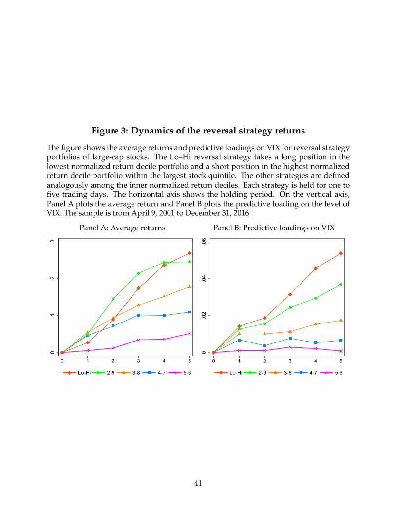
Figure 3: Dynamics of the reversal strategy returns
The figure shows the average returns and predictive loadings on VIX for reversal strategyportfolios of large-cap stocks. The Lo–Hi reversal strategy takes a long position in thelowest normalized return decile portfolio and a short position in the highest normalizedreturn decile portfolio within the largest stock quintile. The other strategies are definedanalogously among the inner normalized return deciles. Each strategy is held for one tofive trading days. The horizontal axis shows the holding period. On the vertical axis,Panel A plots the average return and Panel B plots the predictive loading on the level ofVIX. The sample is from April 9, 2001 to December 31, 2016.
Panel A: Average returns Panel B: Predictive loadings on VIX
0.1
.2.3
0 1 2 3 4 5
Lo-Hi 2-9 3-8 4-7 5-6
0.0
2.0
4.0
6
0 1 2 3 4 5
Lo-Hi 2-9 3-8 4-7 5-6
41

Figure 4: Dynamics of the reversal strategy volatility risk exposure
The figure shows the cumulative exposures to VIX changes and the exposures to day-1 VIX changes for reversal strategy portfolios of large-cap stocks. The Lo–Hi reversalstrategy takes a long position in the lowest normalized return decile portfolio and a shortposition in the highest normalized return decile portfolio within the largest stock quintile.The other strategies are defined analogously among the inner normalized return deciles.Each strategy is held for one to five trading days. The horizontal axis shows the hold-ing period. On the vertical axis, Panel A plots the cumulative betas with respect to VIXchanges, Panel B plots the cumulative betas while controlling for the market return (see18). Panels C and D plot only the betas with respect to VIX changes one day after portfolioformation (βp,VIX
1 in (18)). The sample is from April 9, 2001 to December 31, 2016.
Panel A: Cumulative exposure to ∆VIX Panel B: Cumulative exposureto ∆VIX, controling for RM
-.8-.6
-.4-.2
0
0 1 2 3 4 5
Lo-Hi 2-9 3-8 4-7 5-6
-.8-.6
-.4-.2
0
0 1 2 3 4 5
Lo-Hi 2-9 3-8 4-7 5-6
Panel C: Exposure to day-1 ∆VIX Panel D: Exposure today-1 ∆VIX, controling for RM
-.25
-.2-.1
5-.1
-.05
0
0 1 2 3 4 5
Lo-Hi 2-9 3-8 4-7 5-6
-.15
-.1-.0
50
.05
0 1 2 3 4 5
Lo-Hi 2-9 3-8 4-7 5-6
42

Figu
re5:
Fam
a-M
acB
eth
regr
essi
ons:
aver
age
vers
uspr
edic
ted
retu
rns
The
figur
esh
ows
aver
age
and
pred
icte
dre
turn
sfr
omFa
ma-
Mac
Beth
regr
essi
ons
ofth
efiv
e-da
yre
vers
alpo
rtfo
lios.
Inth
efir
stst
age,
we
regr
ess
the
port
folio
retu
rns
onth
em
arke
tre
turn
and
the
chan
gein
the
VIX
inde
xon
each
day
ofth
eho
ldin
gpe
riod
.W
eth
ensu
mth
eco
effic
ient
sto
obta
inpo
rtfo
lio-l
evel
beta
s.In
the
seco
ndst
age,
we
regr
ess
the
port
folio
retu
rns
onth
ese
beta
s(w
itho
utan
inte
rcep
t)to
obta
infa
ctor
prem
ia.
The
pane
lspl
otth
eav
erag
ere
turn
sof
long
-sho
rtre
vers
alst
rate
gies
(the
rear
efiv
eof
thes
efo
rea
chsi
zequ
inti
le)a
gain
stth
eir
pred
icte
dre
turn
sba
sed
onth
eFa
ma-
Mac
Beth
regr
essi
ones
tim
ates
.The
sam
ple
isfr
omA
pril
9,20
01to
Dec
embe
r31
,201
6.
(1)M
arke
tonl
y(2
)Mar
keta
nd∆
VIX
0.4.81.2Average return
0.4
.81.
2Pr
edic
ted
retu
rn
Smal
l2
34
Big
0.4.81.2Average return
0.4
.81.
2Pr
edic
ted
retu
rn
Smal
l2
34
Big
43

Figu
re6:
Fam
a-M
acbe
thre
gres
sion
sw
ith
are
stri
cted
pric
eof
risk
:ave
rage
vers
uspr
edic
ted
retu
rns
The
figur
esh
ows
aver
age
and
pred
icte
dre
turn
sfr
omFa
ma-
Mac
Beth
regr
essi
ons
wit
ha
rest
rict
edpr
ice
ofri
skba
sed
onth
ere
turn
sof
the
VIX
and
near
-ter
mV
IX(V
IXN
)rep
licat
ing
port
folio
s.Th
ere
stri
cted
pric
eof
risk
isob
tain
edby
divi
ding
the
aver
age
VIX
and
VIX
Nre
turn
sby
thei
rbe
tas
wit
hre
spec
tto
chan
ges
inV
IXan
dV
IXN
,res
pect
ivel
y(s
eeTa
ble
2).T
hepr
ice
ofm
arke
tris
kis
just
the
aver
age
mar
ketr
etur
nov
erth
esa
mpl
e.Th
ese
rest
rict
edpr
ices
ofri
skar
em
ulti
plie
dby
the
beta
sof
the
reve
rsal
port
folio
sw
ith
resp
ectt
oth
em
arke
tand
VIX
orV
IXN
chan
ges
(as
repo
rted
inTa
ble
5).T
his
give
sa
pred
icte
dre
turn
for
each
reve
rsal
port
folio
.The
pane
lspl
otth
eav
erag
ere
turn
sof
long
-sho
rtre
vers
alst
rate
gies
(the
rear
efiv
eof
thes
efo
rea
chsi
zequ
inti
le)a
gain
stth
eir
pred
icte
dre
turn
s.Th
esa
mpl
eis
from
Apr
il9,
2001
toD
ecem
ber
31,2
016.
Mar
keta
nd∆
VIX
Mar
keta
nd∆
VIX
N
0.4.81.2Average return
0.4
.81.
2Pr
edic
ted
retu
rn
Smal
l2
34
Big
0.4.81.2Average return
0.4
.81.
2Pr
edic
ted
retu
rn
Smal
l2
34
Big
44