Liquid-Liquid Extraction With and Without a...
27
10 Liquid-Liquid Extraction With and Without a Chemical Reaction Claudia Irina Koncsag 1 and Alina Barbulescu 2 1 University of Warwick 2 “Ovidius” University of Constanta 1 United Kingdom 2 Romania 1. Introduction The extraction of mercaptans with alkaline solution is accompanied by a second- order instantaneous reaction. As explained in Section 2.2, in this case, the mass transfer coefficients can be calculated as for the physical extraction, since the mass transfer is much slower than the reaction rate.The liquid-liquid extraction is a mass transfer process between two phases. One liquid phase is the feed consisting of a solute and a carrier. The other phase is the solvent. The extraction is understood to be a transfer of the solute from the feed to the solvent. During and at the end of the extraction process, the feed deprived of solute becomes a raffinate and the solvent turns into extract. Extraction is a separation process aiming to purify the feed or to recover one or more compounds from it. The mass transfer mechanism can be described by the well known double film theory, the penetration theory or the surface renewal theory. Especially the stationary double film theory describes most accurately the liquid-liquid extraction. With the means of this theory, the dimensioning of the extraction equipment can be done. Sometimes, over the physical extraction process, a chemical reaction is superposed. Depending on the reaction rate compared with the mass transfer rate, the process can be considered driven by the mass transfer or by the chemical reaction. Also, in some cases, the chemical reaction has an effect of enhancement for the extraction, contributing to speed up the process. As a consequence, the dimensioning of the equipment is different. Many studies have been performed in the last decades for the mathematical modelling of the processes. Accurate correlations between physical properties (densities, density difference, interfacial tension), and dimensions involved in the extraction equipment dimensioning: the drop size diameter, the characteristic velocity of the drop and the slip velocity of the phases were worked out. A smaller number of correlations are available for the calculation of the mass transfer coefficients. Some of the elements needed for the dimensioning of the extractors would be determined experimentally, if a certain accuracy is expected. The experiment is compulsory for the mass transfer coefficients when a new type of equipment is used. The present work exemplifies the theoretical aspects of the liquid-liquid extraction with and without a chemical reaction and the dimensioning of the extractors with original www.intechopen.com
Transcript of Liquid-Liquid Extraction With and Without a...

10
Liquid-Liquid Extraction With and Without a Chemical Reaction
Claudia Irina Koncsag1 and Alina Barbulescu2 1University of Warwick
2“Ovidius” University of Constanta 1United Kingdom
2Romania
1. Introduction
The extraction of mercaptans with alkaline solution is accompanied by a second- order instantaneous reaction. As explained in Section 2.2, in this case, the mass transfer coefficients can be calculated as for the physical extraction, since the mass transfer is much slower than the reaction rate.The liquid-liquid extraction is a mass transfer process between two phases. One liquid phase is the feed consisting of a solute and a carrier. The other phase is the solvent. The extraction is understood to be a transfer of the solute from the feed to the solvent. During and at the end of the extraction process, the feed deprived of solute becomes a raffinate and the solvent turns into extract. Extraction is a separation process aiming to purify the feed or to recover one or more compounds from it. The mass transfer mechanism can be described by the well known double film theory, the
penetration theory or the surface renewal theory. Especially the stationary double film
theory describes most accurately the liquid-liquid extraction. With the means of this theory,
the dimensioning of the extraction equipment can be done.
Sometimes, over the physical extraction process, a chemical reaction is superposed.
Depending on the reaction rate compared with the mass transfer rate, the process can be
considered driven by the mass transfer or by the chemical reaction. Also, in some cases, the
chemical reaction has an effect of enhancement for the extraction, contributing to speed up
the process. As a consequence, the dimensioning of the equipment is different.
Many studies have been performed in the last decades for the mathematical modelling of
the processes. Accurate correlations between physical properties (densities, density
difference, interfacial tension), and dimensions involved in the extraction equipment
dimensioning: the drop size diameter, the characteristic velocity of the drop and the slip
velocity of the phases were worked out. A smaller number of correlations are available for
the calculation of the mass transfer coefficients. Some of the elements needed for the
dimensioning of the extractors would be determined experimentally, if a certain accuracy is
expected. The experiment is compulsory for the mass transfer coefficients when a new type
of equipment is used.
The present work exemplifies the theoretical aspects of the liquid-liquid extraction with and without a chemical reaction and the dimensioning of the extractors with original
www.intechopen.com

Mass Transfer in Multiphase Systems and its Applications
208
experimental work and interpretations. The experiment involved extraction of acid compounds from sour petroleum fractions with alkaline solutions in structured packing columns. Such an example is useful for understanding the principles of dimensioning the extraction equipment but also offers a set of experimental data for people developing processes in petroleum processing industry. A simple, easy to handle model composed by two equations was developed for the mercaptans (thiols) extraction.
2. Theoretical aspects
The immiscible liquid phases put in contact (the feed and the solvent) form a closed system evolving towards the thermodynamic equilibrium. According to the Gibbs law:
2 3 2 2 3l c f= + − = + − = , (1)
the system can be defined by three parameters (l=3), the number of components being c=3
(solvent, solute and carrier), and the phases number f=2. Usually, the parameters taken into
account are the temperature (T), the concentration of the solute in the raffinate (x) and the
concentration in the extract (y). So, the equilibrium general equation in this case is:
( )t consty f x == (2)
The equilibrium equation can have different forms, but most frequently, if the liquid phases
are completely immiscible and the solute concentration is low, the Nernst law describes
accurately the thermodynamic equilibrium:
y m x= ⋅ , (3)
where m is the repartition coefficient of the solute between the two phases. The Nernst law
can be applied also at higher concentration of the solute but in a narrow range of
concentrations.
yA
yAi
xAi
xA
yA
yAi
xAi
xA
yAi
xAi
a) b) c)
Fig. 1. The evolution of the solute concentration in the vicinity of the interface in a closed system
The double stationary film theory of Whitman leads to very good practical results for the
determination of mass transfer coefficients. According to this theory, the phases are
separated by an interface and a double film (one of each phase) adheres to this interface. The
www.intechopen.com

Liquid-Liquid Extraction With and Without a Chemical Reaction
209
mass transfer takes place exclusively in this double stationary film by the molecular
diffusion mechanism. In the bulk of both phases, the concentration of the solute is
considered uniform as a consequence of perfect mixing.
In Fig.1, the evolution in time is presented for a closed system approaching the equilibrium, in the light of double film theory. Notations xAi and yAi are for the concentration at the interface in raffinate and extract respectively; xA and yA denote the concentration of the solute A in the bulk of the raffinate and of the extract respectively. In Fig.1, the mass transfer is presented in a closed system in evolution from the initial state a to the final equilibrium state c. The concentrations at the interface are constant and linked by the equilibrium equation since the concentration of the solute in the bulk feed /raffinate decreases and the concentration of the solute in the bulk solvent/ extract increases in time until equalling the equilibrium concentrations. If the system is open, yA and xA are constant in time (the regime becomes stationary) and the system is maintained in the state a.
2.1 Mass transfer coefficients in physical extraction
In liquid-liquid extraction, the best mechanism describing the mass transfer is the unicomponent diffusion (the solute A diffusing in one direction without a counter diffusion). According to Maxwell- Stefan model, the mass transfer rate in the raffinate film is:
( )(1 )
R ARA A Ai
R A ml
c DN x x
l x= −−
⋅ (4)
In the Eq.4, NA is the flow of component A transferred from the raffinate through the film to the interface; DAR is the diffusion coefficient of the solute in the raffinate phase; cR is the total concentration of components in the raffinate, usually expressed as kmol/m3; lR is the
thickness of the raffinate film; (1 )
R AR
R A ml
c D
l x−⋅
denoted with kR is the partial mass transfer
coefficient in the raffinate phase and 1/kR is the resistance to the transfer. Similarly, Eq.5 describes the mass transfer rate in the extract film, E being the notation for “extract”:
( )(1 )
E AEA Ai A
E A ml
c DN y y
l y= −−
⋅ (5)
During a stationary regime, the component A doesn’t accumulate in the raffinate film as well as in the extract film; this means that the flux transferred in the raffinate film to the interface equals the flux transferred from the interface into the extract phase:
( ) ( )A E Ai A R A AiN k y y k x x= − = − (6)
In Eq.6, (yAi-yA) and (xA-xAi) are the driving forces of the mass transfer in the extract film and in the raffinate film respectively (related to the partial mass transfer coefficients). These
partial driving forces can be read on the axes in the Fig. 2, where the system state is represented by the point A and the equilibrium concentrations at the interface are represented by the point Ai. The arrow AAi denotes the distance from the actual state of the
system to the equilibrium state. But the overall driving force is (xA-xAe), related to the raffinate phase and (yAe- yA), related to the extract respectively. The overall driving forces
www.intechopen.com

Mass Transfer in Multiphase Systems and its Applications
210
refer to the distance from the actual state of the system to an hypothetical state when the actual concentration of the raffinate (xA) would be in equilibrium with the extract (yAe), or the actual concentration of the extract (yA) would be in equilibrium with the raffinate (xAe).
Fig. 2. The representation of the driving forces for the mass transfer (immiscible liquid phases; equilibrium described by Nernst law)
In connection with the overall driving forces, the overall mass transfer coefficients are defined in the equations (7) and (8):
( )A R A AeN K x x−⋅= (7)
( )A E Ae AN K y y−⋅= (8)
As seen in Fig.2, the slope of the equilibrium curve (m) can be calculated from geometrical dimensions (Eq.9):
Ai A AE A AE Ai
Ai Ae A Ae A Ai
y y y y y ym
x x x x x x
− − −= = =− − − (9)
By manipulating the Eq.6-9 and Fig.2, the Eq.(10) and (11) are obtained and would be used for the calculation of the overall mass transfer coefficients KR and KE [m.s-1] when the partial coefficients kR and kE are known:
1 1 1
R R EK k m k= + ⋅ (10)
1 1
E E R
m
K k k= + (11)
More often, the mass transfer coefficients are not related to the raffinate/ extract phases but
more important, to the continuous and the dispersed phase. The extraction system is in fact
an emulsion: one of the phases is in form of droplets and the other one is continuous. Which
Ai
A
y=m x
xAe xAi xA x
y yAe
yAi
yA 0
www.intechopen.com
Liquid-Liquid Extraction With and Without a Chemical Reaction
211
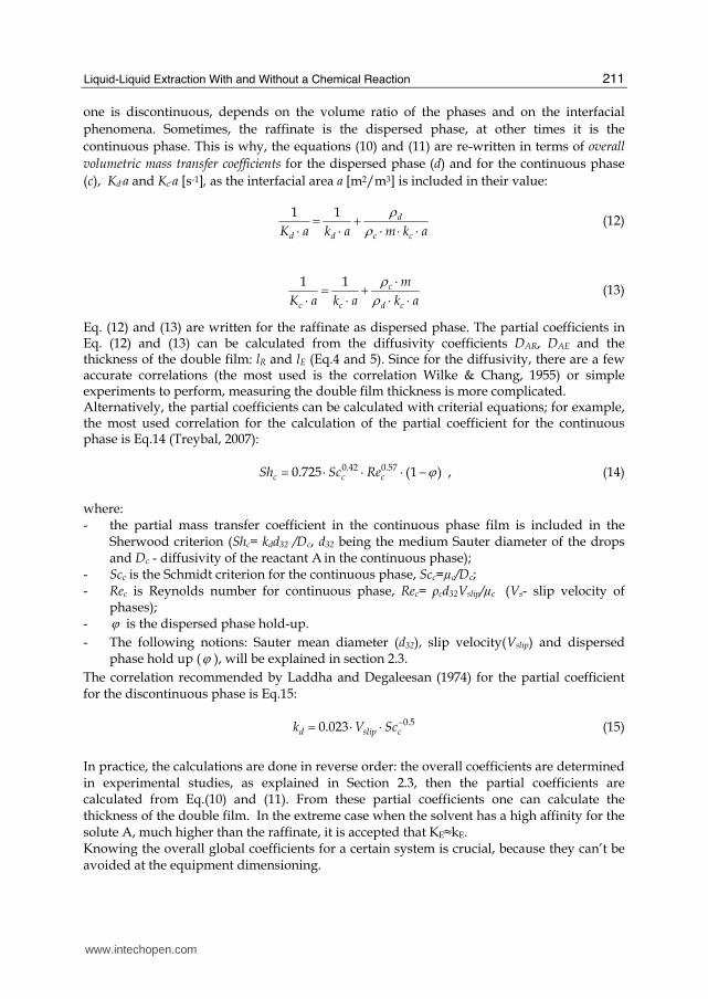
one is discontinuous, depends on the volume ratio of the phases and on the interfacial
phenomena. Sometimes, the raffinate is the dispersed phase, at other times it is the
continuous phase. This is why, the equations (10) and (11) are re-written in terms of overall
volumetric mass transfer coefficients for the dispersed phase (d) and for the continuous phase
(c), Kd.a and Kc.a [s-1], as the interfacial area a [m2/m3] is included in their value:
1 1 d
d d c cK a k a m k a
ρρ= + ⋅⋅ ⋅ ⋅ ⋅ (12)
1 1 c
c c d c
m
K a k a k a
ρρ= + ⋅
⋅ ⋅ ⋅ ⋅ (13)
Eq. (12) and (13) are written for the raffinate as dispersed phase. The partial coefficients in Eq. (12) and (13) can be calculated from the diffusivity coefficients DAR, DAE and the thickness of the double film: lR and lE (Eq.4 and 5). Since for the diffusivity, there are a few accurate correlations (the most used is the correlation Wilke & Chang, 1955) or simple experiments to perform, measuring the double film thickness is more complicated. Alternatively, the partial coefficients can be calculated with criterial equations; for example, the most used correlation for the calculation of the partial coefficient for the continuous phase is Eq.14 (Treybal, 2007):
0.42 0.570.725 (1 )c c cSh Sc Re ϕ⋅ ⋅= ⋅ − , (14)
where: - the partial mass transfer coefficient in the continuous phase film is included in the
Sherwood criterion (Shc= kdd32 /Dc, d32 being the medium Sauter diameter of the drops and Dc - diffusivity of the reactant A in the continuous phase);
- Scc is the Schmidt criterion for the continuous phase, Scc=µc/Dc; - Rec is Reynolds number for continuous phase, Rec= ρcd32Vslip/µc (Vs- slip velocity of
phases); - ϕ is the dispersed phase hold-up.
- The following notions: Sauter mean diameter (d32), slip velocity(Vslip) and dispersed phase hold up (ϕ ), will be explained in section 2.3.
The correlation recommended by Laddha and Degaleesan (1974) for the partial coefficient for the discontinuous phase is Eq.15:
0.50.023d slip ck V Sc−⋅= ⋅ (15)
In practice, the calculations are done in reverse order: the overall coefficients are determined in experimental studies, as explained in Section 2.3, then the partial coefficients are calculated from Eq.(10) and (11). From these partial coefficients one can calculate the thickness of the double film. In the extreme case when the solvent has a high affinity for the solute A, much higher than the raffinate, it is accepted that KE≈kE. Knowing the overall global coefficients for a certain system is crucial, because they can’t be avoided at the equipment dimensioning.
www.intechopen.com

Mass Transfer in Multiphase Systems and its Applications
212
2.2 Mass transfer coefficients in chemical extraction
Let’s consider a reaction in the liquid-liquid system:
A+q. B→ Products
The first phase contains the component A which diffuses from the first phase into the second one containing B, reacting with B in that phase. Then, products diffuse in the same phase 2. Reactions in liquid-liquid systems can be classified from kinetically point of view as slow, fast and instant (Sarkar et al, 1980). The equation describing the diffusion of the reactant A simultaneously with the chemical reaction is (Astarita, 1967):
2 AA RA
cu c v
tA AD c
∂∇ = ⋅∇ + +⋅ ∂ (16)
The term on the left hand side of the Eq.16 represents the molecular diffusion of the component A through the film of phase 1, The terms on the right hand sides have the following meaning: the first one describes the transport by convection through the same film, the second one is the accumulation of A in the film and the third represents the reaction rate. The Eq. 16 can be simplified in the conditions of the double film theory, where the diffusion direction of A is perpendicular to the interface (direction x), eddies are inexistent in the film and component A doesn’t accumulate in the film:
2
2A
A RA
d cD v
dx=⋅ (17)
The Eq.17 can be detailed for both reactants:
2
2A A
A
d c dcD
dtdx=⋅ (18)
2
2B B
B
d c dcD
dtdx=⋅ (19)
Fast and instant reactions In case of fast and instant reactions, the reaction takes place in the plane located in the film of phase 2 (phase containing the component B). The component A diffuses through the film 1 to the interface then from interface to the reaction plane (see Fig. 3 a). In Fig.3 a, a particular case of fast reaction: the irreversible instantaneous reaction is illustrated; in this case, both reactants diffuse to the reaction plane, where their concentrations equals to zero. The term “instantaneous” is idealised since the reaction rate is always finite, but in this case, the mass transfer rate is much lower than the reaction rate, so the process is entirely controlled by the diffusion mechanism. Taking into account the position of the reaction plane (at the distance ┣ from the interface) and the stoechiometric coefficient of the reaction q, the Eq.18 and 19 considering their equality, and integrating, the Eq. 20 is obtained:
1A B
A Bx x
dc dcD D
dx q dxλ λ= =⎛ ⎞ ⎛ ⎞= ⋅⎜ ⎟ ⎜ ⎟⎝ ⎝ ⎠⋅ ⋅⎠ . (20)
www.intechopen.com

Liquid-Liquid Extraction With and Without a Chemical Reaction
213
Phase 1 Phase 2
δ1 0 δ2
cA0
cB0
cA1i
cA2i
λPhase 1 Phase 2
δ1 0 δ2
cA0
cB0
cA
*
cA1i
cA2i
(a) (b)
Fig. 3. Profiles of reactants concentration at the extraction with a chemical reaction: a - instantaneous irreversible reaction taking place in phase film 2; b - slow reaction taking place in the film phase 2
By integrating Eq.20 between the limits x=┣ and x=l, (l- the film thickness), it results:
2 0A i BA B
c cq D D
lλ λ⋅ = ⋅ −⋅ (21)
In Eq.21, cA2i is the concentration of A at the interface on the film’s 2 side and cB0 is the
concentration of B in bulk of the phase 2. The Eq. 21 can be re- written in another form:
2
2 0
A A i
A A i B B
q D cl
q D c D cλ ⋅= ⋅ ⋅ ⋅+
⋅⋅ (22)
l
λ is in fact the ratio between the the overall mass transfer coefficient with a chemical
reaction K.a, and the overall mass transfer coefficient at the physical extraction (without a
chemical reaction), K0.a:
00
2
1 BB
A A i
cK a l D
D q cK a λ= + ⋅ ⋅⋅⋅ = , (23)
So, the overall mass transfer coefficient in the case of instant reaction is proportional to the
coefficient for the physical extraction. It means that the coefficient at the extraction with
instant chemical reaction depends on hydrodynamics in the same extent as that for physical
extraction.
For instantaneous irreversible reactions, the enhancement factor Ei is defined (Pohorecki,
2007) by Eq.24:
( )
( )i
Q instantaneousreactionE
Q physical= (24)
www.intechopen.com

Mass Transfer in Multiphase Systems and its Applications
214
where Q is the quantity transferred through the interface (mol m-2). If this quantity is divided by time, the enhancement factor is defined as the factor by which the reaction increases the overall transfer rate compared to the rate of physical transfer (in the absence of the reaction). Taking into account Eq.23, the enhancement factor at the interface can be calculated by the formula:
0
2
1 BBi
A A i
cDE
D q c= + ⋅ ⋅ (25)
As seen in Eq.25, the enhancement factor can be calculated with the diffusivities of the reactants and their concentrations in bulk of phase and at the interface; because the concentration is difficult to be determined at the interface, the following approach is more feasible: - The overall mass transfer coefficient for the physical extraction of component A from
the phase 1 in phase 2, K0.a, is calculated with Eq.14 or 15, depending on the phase where the reaction takes place; the individual transfer coefficients can be estimated with Eq.16 and 17 or other correlations found in literature (Treybal, 2007 and Pratt, 1983); the slip velocity Vslip intervening in the Eq.15 directly or in Eq.14 in the Reynolds number, can be calculated, as it will be seen in Section 2.3;
- The actual overall mass transfer coefficient including the chemical reaction is determined experimentally, K.a, as it will be seen in Section 2.3;
- The ratio0
K a
K a
⋅⋅ represents the enhancement factor E; it is higher than 1, sometimes >>1,
depending on the physical properties of the system (DA, K0.a) and the constant of reaction rate; the values of E experimentally determined are useful for the calculation of the concentration of the reactant A at the interface cAi (Eq.25) needed in further calculations.
The intensification of the mass transfer during the chemical reaction was explained here in the frame of the film theory but in fact, the renewal of interface theory could better explain what happens: the interfacial tension depends on the concentration of the transferred substance and as a result, spontaneous interfacial convection is initiated, so a more intensive renovation of the interface and, correspondingly, an increase in the mass transfer coefficient is achieved (Ermakov et al, 2001) Slow reactions The slow reaction can take place in the film but more probably, in the bulk of the solvent phase 2. In Fig.3b, the reaction takes place in the film phase 2. The process can be considered a physical diffusion of component A in the phase 2 film followed by reaction between A and B in the film of the phase 2. Unlike the fast reaction, part of component A remains un-reacted and diffuses further in the phase 2, where its concentration is cA*. In Fig.3.b it is illustrated the case when component B is completely consumed in the reaction, but there are more complicated cases when B is not consumed in the film phase 2 but diffuses further in the phase 1 and reaction could take place in one or both phases. In a steady state, there is no accumulation of component A in any point of the system; this means that the rate of physical transfer process equals the consumption rate of A in reaction:
EK a k a⋅ = ⋅ ( *2A i Ac c− ) ( )0 1
1( , )A A i A Bc c r c cτ= − + (26)
www.intechopen.com

Liquid-Liquid Extraction With and Without a Chemical Reaction
215
where 1A ic and 2A ic are the concentrations of A at the interface (see Fig.3) in
thermodynamic equilibrium. The mass transfer depends on the contact time of phases in the
extractor. The contact time is the same as the residence time ┬, defined in Eq.27:
V
Qτ = , (27)
where V is the active volume of the extractor (the volume occupied by the emulsion in the extractor) and Q is the total volumetric flow of the phases.
For the first order irreversible reaction: r= - k1.cA* (k1- reaction rate constant) and taking into
account the equilibrium correlation: 1 2A i A ic m c= ⋅ (m- the repartition coefficient, Eq.3), the
Eq.26 becomes:
( ) ( )* *2 0 2 1
1E A i A A A i AK a k a c c c m c k cτ⋅ = ⋅ − ⋅ ⋅= − − (28)
In the Eq.28, only cA2i can’t be measured, so the equation is re-arranged in all measurable or calculable terms (Sarkar et al, 1980):
⋅K a = *10 1
1 EA A
E
k kc m k c
mk aτ τ
⎛ ⎞⎜ ⎟+⋅ − ⋅ −⎜ ⎟⎜ ⎟−⎜ ⎟⎝ ⎠⋅
⋅ (29)
As seen in Eq.29, the rate of transfer for the extraction with slow reaction, depends both on
the mass transfer coefficient (KE) and on the reaction rate constant (k1). The process is
controlled by the slowest step: the mass transfer or the reaction.
2.3 The dimensioning of the extractors. The column with continuous differential contact of phases
All the theory about the mass transfer coefficients has as a practical goal the dimensioning of
the industrial equipment for liquid-liquid extraction.
Dimensioning and extractor means to find its main geometrical dimensions. As an example,
the column type extractors are presented here but for other type of equipment, the
dimensioning is very different (Godfrey & Slater, 1994). Dimensioning a column means to
find its diameter and height.
For the columns with continuous differential contact, the phases flow in countercurrent, one
of the phases being continuous, the other one dispersed (drops).
2.3.1 The column diameter
The diameter of the column is correlated with the processing capacity of the column (the
flow of the phases) and the flooding capacity. The synthetic form of this correlation was
expressed by Zhu and Luo (1996):
4 ( )c d
cmax
Q QD
k Bπ⋅ += ⋅ ⋅ (30)
www.intechopen.com

Mass Transfer in Multiphase Systems and its Applications
216
where: Qc is the continuous phase volumetric flow, [m3.s-1] Qd- the dispersed phase volumetric flow, [m3.s-1] Bmax is the flooding capacity, [m3.m-2.s-1]; considering the flow in the free cross-sectional area of the column. The flooding capacity Bmax is in fact the sum of the flooding velocities of phases; it depends on the physical properties of the system: the density (ρc and ρd), the viscosity (µc and µd) and the interfacial tension ┫. The flooding capacity can be predicted following extensive studies, as exemplified in Section 3. k- the flooding coefficient, with values from 0.4 (dispersion column) to 0.8 (column equipped with structured packing); this coefficient would be kept as high as possible, in order to increase the mass transfer rate and the processing capacity of the column. The flooding capacity is experimentally determined for each type of column. It consists in derangements of the countercurrent flow bringing about entrainment of one phase in the other one, or the impossibility for one flow to enter the column. There are three main mechanisms of flooding: - The phase inversion provoked by the excessive increasing of dispersed phase flow; - The entrainment of the drops in the continuous phase when the flow of continuous
phase increases too much; - The flooding due to the contaminants at the interface creating instability of the interface
of even inversion of the phases.
According to authors after Hanson (1971), the diameter calculation is made using the
concept of slip velocity, Vslip, which is the velocity of the dispersed phase related to the
continuous phase; the slip velocity is in fact, the sum of linear velocities of the phases, not in
the free cross-sectional area but in the actual cross-sectional area, taking into account the
internal parts of the column and the dispersed phase holdup, φ . According to this
definition, in the dispersion column (without any internal parts, such as trays or packing),
the slip velocity is:
1
d cslip
V VV φ φ= + − (31)
The dispersed phase holdup is the fraction occupied by the drops in the free cross sectional area of the column. In fact, the holdup is not uniformly distributed in the column because the drops are of various dimensions, with an irregular shape, oscillating. For approximate calculations, a mean diameter would be taken into consideration. The most usual expression of this is the Sauter mean diameter, d32:
3
32 2
i i
i i
n dd
n d= ⋅
⋅∑∑ (32)
The mean diameter d32, is correlated with the holdup φ and the interfacial area a:
32
6a
d
φ⋅= (33)
Empirical correlations can be used to correlate Sauter mean diameter d32 with physical properties of the system. It can be calculated with the formula recommended by Seibert & Fair (1988) and verified by Iacob & Koncsag (1999) on systems with high interfacial tension:
www.intechopen.com

Liquid-Liquid Extraction With and Without a Chemical Reaction
217
0.5
32 1.15dg
σρ
⎛ ⎞= ⎜ ⎟⋅⎝ ⎠J (34)
where Δρ- density difference of phases, g –gravitational constant. It is difficult to determinate the slip velocity, but it can be easier done but an easier by correlating it with the singular drop’s characteristic velocity, VK, which can be determined experimentally. VK is defined as the ratio between the distance travelled by the singular drop in the column and the time of this trip. The singular drop’s characteristic velocity is uninfluenced by the presence of other drops but is influenced by the presence of the internal parts of the equipment. For example, in the case of packed column, VK can be correlated with the physical properties of the liquid-liquid system and the geometrical characteristics of the packing:
0.5
30.637
p cK
aV
g
ρε ρ
−⎛ ⎞= ⎜ ⎟⎜ ⎠⋅ ⎟⋅⎝⋅
J (35)
There are correlations between the slip velocity and the singular drop’s characteristic velocity. A simple correlation is the Pratt- Thornton equation which is valid for rigid (non-oscillating) drops and low values of the holdup (Thornton, 1956):
(1 )slip KV V φ⋅= − (36)
For higher values of holdup, a more accurate equation would be used (Misek, 1994):
( )1 exp( )slip KV V aφ φ= −⋅ (37)
2.3.2 The column height For extractors with countercurrent flow of the phases, the active height is calculated on the basis of the mass transfer unit notion. In the hypothesis of the plug flow, the height of the column is:
[ ][ ] [ ] [ ]od od oc ocH NTU HTU NTU HTU= ⋅ ⋅= (38)
where [NTU]od and [NTU]oc are the number of transfer units relative to the dispersed and to the continuous phase respectively, when expressing the mass transfer rate as the overall mass transfer coefficients. [HTU]od and [HTU]oc are the height of the transfer unit relative to the overall mass transfer coefficient in the same phases. The height of the transfer unit is the height of the column which ensures the decreasing by e (=2.71…) of the driving force defined as in the Eq.7 and 8, taking into account which is the dispersed phase and the continuous one. [NTU]od and [NTU]oc are calculated taking into account the equilibrium data. The relationships given in Eq.39 and 40 are related to the extract (E) and the raffinate (R) and it is to see which equation applies to the continuous phase or the dispersed phase (e.g. the raffinate can be dispersed phase in one application and continuous phase in another one):
2
1
[ ]x
oRex
dxNTU
x x= −∫ (39)
www.intechopen.com

Mass Transfer in Multiphase Systems and its Applications
218
2
1
[ ]
y
oEey
dyNTU
y y= −∫ (40)
where: x1, x2, y1, y2 are the solute concentration in the raffinate (x) and in the extract respectively (y) in the flow entering (1) or exiting (2) the column. xe , ye are the solute concentrations in raffinate and in the extract respectivelly, in
equilibrium conditions in every point along the column.
[HTU]od and [HTU]oc are experimentally found by dividing the active height of the column
(the height of the column where the dispersed phase and the continuous phase co-exists) by
the [NTU]od or [NTU]oc.
Let’s express the mass transfer for the dispersed phase. The volumetric overall mass transfer
coefficients related to the dispersed phase Koda are correlated with the height of the mass
transfer unit [HTU]od and the superficial velocity of the dispersed phase vd (which is defined
as the volumetric flow divided by the cross- sectional area of the column):
dod
od
vK a
HTU=⋅ (41)
In practice, the height of the column is calculated starting with the experimental determination of mass transfer coefficients, continuing by the calculation of HTU with Eq.41 and finally, applying the Eq. 38.
3. Experimental data
The theoretical aspects presented here are very general. In fact, an engineer needs
mathematical models for the dimensioning of the industrial equipment, specific for a given
type of extractor. Here we present the process of the model’s development, using a large
database, partially relying on our original experiment, partially on data from literature, for
the dimensioning of a packed column.
The original experimental data were obtained in a 76 mm diameter column with structured
packing type Sulzer SMV 350 Y. The specific area of the packing was: ap= 340 m2/m3 and the
void fraction ε = 0.96. The packing bed was made of 4 structured packing elements with a
total height of 840 mm. The detailed description of the pilot plant was presented in a
previous work (Koncsag & Barbulescu, 2008). Another type of ordered packing -corrugated
metal gauze- was used in a mass transfer study at laboratory scale, also described in
(Koncsag & Barbulescu, 2008). The experiment at laboratory scale was performed in another
installation including a glass column with the internal diameter of 3 cm and an active height
of 70 cm. The handicraft packing was made of corrugated metal gauze and had the
following geometric characteristics: ε = 0.98 and ap = 60 m2/ m3. Taking into account the
small opening of the spiral, the drops are forced to detour and the tortuosity of their motion
increases; as a consequence, the residence time of the drops in the column increases and the
mass transfer improves comparing with the simple dispersion column. Also, the experiment
was performed for the dispersion column (the column unpacked).
So, three sets of data were obtained: for the Sulzer SMV350 packing, for the corrugated
metal gauze packing and without packing (Table1).
www.intechopen.com

Liquid-Liquid Extraction With and Without a Chemical Reaction
219
The studied systems were: water– gasoline, NaOH solution 20%wt – gasoline and carbon tetrachloride– water. These systems were very different from the viewpoint of density, interfacial tension and viscosity. The first and the third systems are usually taken into account in the hydrodynamic studies and the second one is common in the purifying of hydrocarbon streams. The results of the flooding tests are expressed as pairs of limiting superficial velocities of the phases (continuous and dispersed), in flooding conditions: Vcf, Vdf. Other experimental data from the literature were connected to the results of the original
experiment (Table 1), in order to have a larger database for the mathematical model (Table 2).
The data were chosen for hydrocarbon – water systems (gasoline- water or toluene- water) and
for very different types of packing: Raschig rings of different size (Crawford & Wilke, 1951);
Norton ordered packing (Seibert & Fair, 1988) and Intalox saddles (Seibert et al, 1990).
Flooding superficial velocities for the system gasoline- water , d32 = 0.0052 m, ρc=996 kg/m3, ρd=740 kg/m3, ┤c= 0.000993 kg/m. s, σ= 52.0.10-3N/m , vK= 0.055 m/s
1 2 3 4 5
0.88 0.84 0.69 0.32 0.21
0.17 0.27 0.43 0.84 1.00
Flooding superficial velocities for the system gasoline- 20%NaOH solution, d32 = 0.0047 m, ρc=1220 kg/m3, ρd=740 kg/m3, ┤c= 0.00366 kg/m. s, σ= 78.6 .10-3N/m, vK= 0.067 m/s
1 2 3 4 5
0.80 0.68 0.43 0.32 0.27
0.11 0.17 0.84 1.17 1.31
Flooding superficial velocities for the system water – CCl4 at 5oC, d32 = 0.0035 m, ρc=1610 kg/m3, ρd=996kg/m3 , ┤c= 0.00123 kg/m. s, σ= 47.3 .10-3N/m, vK= 0.0604 m/s
1 2 3 4 5
0.64 0.62 0.58 0.35 0.24
0.17 0.27 0.37 1.17 1.43
Table 1. Experimental data at the hydrodynamic test in the column equipped with Sulzer packing (ap= 340 m2/m3, ε=0.96, Dcol = 0.076 m)
The second part of the experiment consisted of a mass transfer study concerning the extraction of mercaptans from petroleum fractions with alkaline solutions, a process encountered in the oil processing industry. The raw material was the gasoline enriched in mercaptans (ethanethiol or 1-propanethiol or
1-buthanethiol) and pumped into the column where it forms the dispersed phase; after the
extraction and the coalescence, the gasoline exits the column at the top, as a refined phase.
The solvent – the continuous phase- is in fact a caustic solution (NaOH) with concentration
in range of 5-15% wt. The continuous phase enters the column free of mercaptans and exits
as an extract enriched in the said mercaptans. Samples of feed and refined phase are
www.intechopen.com

Mass Transfer in Multiphase Systems and its Applications
220
collected and the mercaptans concentration is analyzed by a volumetric method using
AgNO3. The concentration of the mercaptans in the extract is calculated by material balance.
The volumetric overall mass transfer coefficients were calculated byEq.37, 38 and 40 and are
presented in Table 3.
Flooding superficial velocities for the system gasoline- water in case of the contactor equipped with Raschig rings 1/ 2” (ap= 310 m2/m3, ε=0.71, Dcol = 0.305 m) ,d32 = 0.0052 m, ρc=996 kg/m3, ρd=740 kg/m3 , ┤c= 0.000993 kg/m. s, σ= 42.4 .10-3N/m, vK= 0.037 m/s
Superficial velocities of phases, m/s 1 2 3 4
102. Vdf 0.88 0.58 0.38 0.13
102. Vcf 0.25 0.44 0.60 0.97
Flooding superficial velocities for the system gasoline- water in case of the contactor equipped with Raschig rings 1” (ap= 195 cm2/cm3, ε=0.74, Dcol = 0.305 cm); d32 = 0.0052 m, ρc=996 kg/m3, ρd=740 kg/m3 , ┤c= 0.000993 kg/m. s, σ= 42.4 .10-3N/m, vK= 0.05 m/s
Superficial velocities of phases, m/s 1 2 3 4 5
102. Vdf 1.64 1.10 0.88 0.67 0.36
102. Vcf 0.54 0.83 1.00 1.23 1.69
Flooding superficial velocities for the system toluene- water in case of the contactor equipped with Norton packing (ap= 213 m2/m3, ε=0.97, Dcol = 0.425 m);d32 = 0.0055 m, ρc=996 kg/m3, ρd=864 kg/m3, ┤c= 0.00089 kg/m. s, σ= 30.0 .10-3N/m, vK= 0.0497 m/s
Superficial velocities of phases, m/s 1 2 3 4 5
102. Vdf 1.13 0.93 0.72 0.60 0.30
102. Vcf 0.9 1.01 1.14 1.30 1.60
Flooding superficial velocities for the system toluene- water in case of the contactor equipped with Intalox saddles No25 IMTP (ap= 226 m2/m3, ε=0.95, Dcol = 0.102 m); d32 = 0.0055 m, ρc=996 kg/m3, ρd=864 kg/m3, ┤c= 0.00089 kg/m. s, σ= 30.0 .10-3N/m, vK= 0.0477 m/s
Superficial velocities of phases, m/s 1 2 3 4 5
102. Vdf 1.44 1.32 0.93 0.72 0.51
102. Vcf 0.79 1.05 1.40 1.58 1.75
Table 2. Experimental data from literature concerning the hydrodynamic tests in the columns equipped with other type of packing
4. Discussion
The original experimental data about the flooding- linked to the column capacity- (Table 1) were compared with the predicted data from older models in the literature for packed columns, in order to see if they are satisfactory models or should be improved. If not, a new model would be developed.
4.1 The Crawford-Wilke model
A good old model is the Crawford– Wilke correlation curve (Crawford & Wilke, 1951). At the
beginning, this model correlated a total of 160 experimental points for a large range of random
packing but relatively few liquid systems.
www.intechopen.com

Liquid-Liquid Extraction With and Without a Chemical Reaction
221
Dispersion column Laboratory packed column Pilot packed column
NaOH conc.
Dispesed phase
velocity, Vd
(x102,m/s)
Koda (x103,s-1)
Dispesed phase
velocity, Vd
(x102,m/s)
Koda (x103,s-1)
Dispesed phase
velocity, Vd
(x102, m/s)
Koda (x103,s-1)
0.17 0.91 0.17 1.25 0.21 3.0
0.23 1.06 0.25 1.43 0.43 4.5
5%
0.33 1.16 0.33 2.05 0.68 6.5
0.17 0.89 0.17 1.56 0.21 3.1
0.23 1.20 0.25 1.93 0.43 4.8
10% 0.33 1.38 0.33 2.87 0.68 7.1
0.17 1.49 0.17 1.93 0.21 3.1
0.23 1.74 0.25 2.47 0.43 3.7
Bu
than
eth
iol
15%
0.33 2.19 0.33 2.54 0.68 7.0
0.13 1.64 0.13 1.69 0.21 5.4
0.20 1.66 0.20 2.17 0.32 7.8
5% 0.26 1.77 0.26 2.62 0.68 13.1
0.13 1.53 0.13 1.94 0.21 6.3
0.20 1.98 0.20 2.23 0.32 10.2
10%
0.26 2.08 0.26 2.32 0.68 13.8
0.13 2.34 0.13 2.85 0.21 7.1
0.20 2.65 0.20 3.08 0.32 11.2
Pro
pan
eth
iol
15%
0.26 2.73 0.26 3.94 0.68 16.1
0.17 2.78 0.17 6.02 0.21 8.3
0.23 3.66 0.23 6.27 0.32 11.4
5% 0.33 4.31 0.33 8.34 0.58 18.2
0.17 5.06 0.17 6.45 0.21 9.3
0.23 5.36 0.23 8.26 0.32 13.3
10% 0.33 8.21 0.33 13.87 0.58 22.2
0.17 5.77 0.17 7.84 0.21 10.2
0.23 6.43 0.23 10.30 0.43 19.2
Eth
anet
hio
l
15%
0.33 11.67 0.33 14.46 0.68 28.6
Table 3. Experimental data at the mercaptans extraction
www.intechopen.com

Mass Transfer in Multiphase Systems and its Applications
222
This model started from the premise that the sum of the square roots of the flooding velocity of both phases is a constant. This seemed reasonable for a large range of packing and systems, even that it has no a theoretical basis. The sum: (Vcf1/2+Vdf1/2)2 = constant, is correlated with the physical properties of the liquids and the characteristics of the packing
(ap, ε):
1 10.22 2( )cf df pc
p c c
V V af
a
ρ μσμ ρ ρ ε
⎡ ⎤+ ⋅ ⎛ ⎞⎛ ⎞ ⎛ ⎞⎢ ⎥= ⎜ ⎟⎜ ⎟ ⎜ ⎟⎜ ⎟⎢ ⎥⎝ ⎠⎝ ⎠ ⎝ ⎠⎣ ⎦⋅ J (42)
The variables of Eq.42 are plotted in Figure 4.
Y
10000
5000
2000
1000
500
200
100
50
20
10
1 2 5 10 20 50 100 200 500 1000, X
Y
10000
5000
1000
500
200
100
50
20
10
1 2 5 10 20 50 100 200 500 1000, X*
(a) (b)
Fig. 4. The correlation between the flooding velocity of the phases - the Crawford-Wilke
model. Legend: a- the original correlation (
1/2 1/2cf dj
p c
(V V ) ρX
a ┤+ ⋅⋅= ,
1.50.2 1.0pc
c
a┤σY
ρ ρ ε⎛ ⎞⎛ ⎞ ⎛ ⎞= ⎜ ⎟⎜ ⎟ ⎜ ⎟ ⎜ ⎟⎝ ⎠⎝ ⎠ ⎝ ⎠J
);
b- the modified correlation ( [ ] [ ]1/2 1/21 p ccf df
* ( k ) ρ) /(a )X V V= + ⋅ ⋅μ ; square for the system
water– gasoline, circle for the system NaOH solution– gasoline and triangle for the system CCl4– water
As one can see from Figure 4.a, our experimental points are pretty far from the original curve. Other authors (Nemunaitis et al 1971) reported the same. They found that flooding occurred at loading only 20% of those predicted by the flooding correlation of Crawford and Wilke. An explanation could be that the assumption of the sum (Vcf1/2+Vdf1/2) constancy is not true. Even Crawford and Wilke (1951) expressed their doubts, however they considered this hypothesis as reasonable. The sum (Vcf1/2+Vdf1/2) = constant indicates that the curves Vdf1/2 vs Vcf1/2 are lines with a slope of (–1):
Vcf1/2 + Vdf1/2= k2 (43)
Eq. 43 does not describe correctly the flooding line. The sum (Vcf1/2 + Vdf1/2) should be
modified as follows: (Vcf1/2+k1Vdf1/2) with respect to the real slope of the flooding line. In
www.intechopen.com

Liquid-Liquid Extraction With and Without a Chemical Reaction
223
this case, 1k = − 1/m’ where (m‘) is the real slope of the flooding line. For the systems
studied in my experiment, it was found: - k1= 1.17 – for Water–Gasoline; (m‘ = -0.85)
- k1 = 2.44– for NaOH sol.20%wt– Gasoline ; (m‘=-0.41)
- k1 = 2.63– for CCl4 – Water; (m‘= -0.38) As one can see, slope m' is in fact very different from the original (-1). This wasn’t obvious when Crawford and Wilke established their model, because the liquid- liquid systems taken into account at that time were (all) low interfacial tension systems. In the present work, very different systems have been considered, proceeding from present authors‘ original experimental data as well as from other authors’ data, e.g. (Nemunaitis et al 1971,), (Watson et al, 1971), (Seibert & Fair, 1998), (Seibert et al.1990). It is to say that the scientific literature is very poor in flooding data in case of liquid-liquid countercurrent contactors. In order to fit all these data and to have a model responding to systems with very different
physical properties, the Crawford– Wilke correlation should be modified as follows: on the
X– axis would appear the expression 1/2 1/2
1*( )cf df
p c
V k VX
a
ρμ
⋅= ⋅+⋅ instead of the expression
1/2 1/2( ) cf df
p c
V VX
a
ρμ
+ ⋅⋅= .
The k1 constant should be calculated with Eq.43 as recommended by Watson et al (1975):
0.5 0.25 0.25 0.5 11 320.466 c ck dρ σ μ ε+ + + + −⋅ ⋅ ⋅= ⋅⋅ (44)
From Fig. 4b, one can see that it is a better accordance of experimental data with the
Crawford– Wilke model when the real slope of the flooding line is considered. The
maximum error of the modified model for our experimental points was 24%, lower than that
reported by the authors of the original correlation: 35% for their own data.
4.2 The Seibert- Fair model
This model was developed after Eighties, when structure packing type was introduced, but it can be also applied to the random type packing as well. The models presented previously were empirical but this one is analytical, starting from the following assumption: the drops are rigid and spherical, the drop size can be represented by a Sauter mean diameter d32, the axial mixing of the continuous and of the dispersed phase can be neglected. The authors
consider a drop traveling at an angle of ascent θ, in order to avoid the packing surface in its path. In a spray column, the mean angle of ascent is 90o but in a packed column the angle is smaller and depends on the drop size and the packing specific area. The packing increases the droplet velocity and the path length. This can be expressed as a tortuosity factor ξ:
32 / 2pa dξ ⋅= (45)
Manipulation of the classic equations of hydrodynamics and the use of the maximum
theoretical holdup value of 0.52 lead to the final expression of the model:
201.08 [cos ] 0.192
4cf df sV V V
πξ ε−⎛ ⎞⋅ + = ⋅ ⋅⎜ ⎟⎝ ⎠ ⋅ (46)
www.intechopen.com

Mass Transfer in Multiphase Systems and its Applications
224
where Vs0 is the slip velocity of the singular drop in the dispersion column defined by
hydrodynamic Eq. 47:
Vs0 = [(Δρgd32) / (3ρc CD)] 0.5 (47)
The dispersed phase holdup at flooding point fφ depends on the the phases flow ratio and
by consequence, on their superficial velocities ratio (Vd and Vc). Seibert & Fair (1988)
proposed the empirical Eq.48:
( )2
0
4
exp 1.921
d
fc
s ff
V cos
VV
π ξφ ε φ φ
−⎡ ⎤⋅⎛ ⎞⎜ ⎟⎢ ⎥⎝ ⎠⎣ ⎦=⋅ − ⋅ −
⋅−
(48)
This correlation is used especially for the prediction of the holdup at flooding, by trial-error
method.
Legend: square for the system water– gasoline, circle for the system NaOH solution– gasoline and triangle for the system CCl4– water. The Fair- Sibert model was verified by its authors and gave good results for their own data obtained on a small diameter (100 mm) column (Seibert & Fair 1988). At larger scale: 400 mm diameter, the model gave bigger errors (Seibert et al. 1990). Also, the model was verified with data obtained in the original experiment (Koncsag & Stratula 2002) giving a maximum error of 26.4%. The parity plot for the original data is shown in Figure 5. It seems to be a good accordance of the original data with the model but in fact the errors are systematic; for example, in the case of CCl4– water system, the errors go continuously from negative to positive values. This could be explained either by non– reliable data or by a non– reliable model. The authors of the present work tend to consider a non– reliable model as long as the authors of the model themselves had a parity plot which indicated exclusively negative values for the standard errors (Seibert et al.1990).
0 0.1 0.2 0.3 0.4 0.5 0.6 0.7 0.8
V df exp
, cm/s
V df calc , cm/s
0.9
0.8
0.7
0.6
0.5
0.4
0.3
0.2
0.1
Fig. 5. The parity plot: Vdf calc (Seibert -Fair model) vs. original experimental values
www.intechopen.com
Liquid-Liquid Extraction With and Without a Chemical Reaction
225
5. Modelling the removal of mercaptans from liquid hydrocarbon streams in structured packing columns
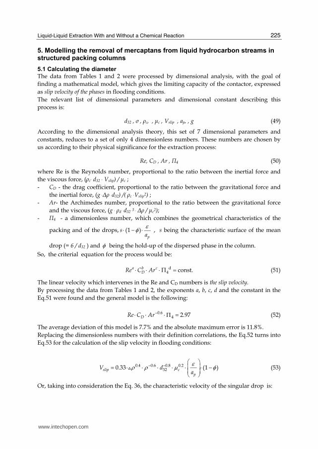
5.1 Calculating the diameter
The data from Tables 1 and 2 were processed by dimensional analysis, with the goal of
finding a mathematical model, which gives the limiting capacity of the contactor, expressed
as slip velocity of the phases in flooding conditions.
The relevant list of dimensional parameters and dimensional constant describing this
process is:
d32 , ┫ , ρc, , ┤c , Vslip , ap, , g (49)
According to the dimensional analysis theory, this set of 7 dimensional parameters and
constants, reduces to a set of only 4 dimensionless numbers. These numbers are chosen by
us according to their physical significance for the extraction process:
Re, CD , Ar , Π4 (50)
where Re is the Reynolds number, proportional to the ratio between the inertial force and
the viscous force, (ρc. d32 . Vslip) / ┤c ;
- CD - the drag coefficient, proportional to the ratio between the gravitational force and
the inertial force, (g .Δρ .d32) /( ρc .Vslip2) ;
- Ar- the Archimedes number, proportional to the ratio between the gravitational force
and the viscous force, (g . ρd .d32 3 . Δρ / ┤c2);
- Π4 - a dimensionless number, which combines the geometrical characteristics of the
packing and of the drops, (1 )p
sa
εφ⋅ − ⋅ , s being the characteristic surface of the mean
drop (= 6 / d32 ) and φ being the hold-up of the dispersed phase in the column.
So, the criterial equation for the process would be:
d4Π const.a b c
DRe C Ar⋅ ⋅ ⋅ = (51)
The linear velocity which intervenes in the Re and CD numbers is the slip velocity.
By processing the data from Tables 1 and 2, the exponents a, b, c, d and the constant in the
Eq.51 were found and the general model is the following:
0.64 2.97DRe C Ar−⋅ Π =⋅ ⋅ (52)
The average deviation of this model is 7.7% and the absolute maximum error is 11.8%.
Replacing the dimensionless numbers with their definition correlations, the Eq.52 turns into
Eq.53 for the calculation of the slip velocity in flooding conditions:
0.4 0.6 0.8 0.2320.33 (1 )slip c
p
V da
ερ ρ μ φ− −⋅ ⋅ ⋅ ⎛ ⎞⎜ ⎟= ⋅ ⋅ −⎜ ⎟⋅ ⎝ ⎠J (53)
Or, taking into consideration the Eq. 36, the characteristic velocity of the singular drop is:
www.intechopen.com

Mass Transfer in Multiphase Systems and its Applications
226
0.4 0.6 0.8 0.2320.33K c
p
V da
ερ ρ μ− − ⎛ ⎞⎜ ⎟= ⋅ ⎜ ⎟⎝⋅ ⋅ ⋅ ⎠⋅J (54)
The new model can serve for dimensioning the liquid- liquid countercurrent contactor
equipped with packing: random or ordered. The steps of the dimensioning are:
- the calculation of the characteristic velocity (Eq.54);
- the choice of the desired ratio of the phases (Vd/Vc);
- the calculation of the dispersed phase holdup by trial- error method (Eq.48);
- the calculation of slip velocity (Eq.53 applied to the flooding conditions, fφ );
- the prediction of the throughputs limit (Vdf and Vcf), knowing their ratio
( d c df cfV / V V / V= ;
- the calculation of the diameter with Eq. 30, where max df cfB V V= + .
5.2 Calculating the active height of the column
The extraction of mercaptans with alkaline solution is accompanied by a second- order
instantaneous reaction. As explained in Section 2.2, in this case, the mass transfer
coefficients can be calculated as for the physical extraction, since the mass transfer is much
slower than the reaction rate.
The calculation of the active height of the column is performed with Eq.38-41. The main
difficulty consists of calculating the integrals (Eq.39 and 40) because one should know the
concentrations profiles along the column. For systems following the Nernst law (Eq.3) and
for very high values of the extraction factor (defined by Eq.56), the number of the transfer
units NTUod can be calculated from the number of theoretical stages NTT, with the Eq.55:
11
od
NTT ENTU lnE
−= (55)
NTT can be found graphically in a McCabe-Thiele- type construction. The extraction factor E is defined by the Eq.56:
S
E mA
= ⋅ (56)
where S/A is the solvent- to- feed gravimetric ratio.
As seen in Eq.56, the phase ratio refers to the solvent and feed and not to dispersed and
continuous, as in diameter calculation. In mass transfer, the direction of the transfer is very
important. Always, the direction is from the feed to the solvent, whatever the dispersed
phase is.
The data used in modelling the extraction of the buthanethiol, propanethiol and ethanethiol
are given in Table 3.
A model of the same type for all the data in Table 3 was developed, taking into account the
factors determining the mass transfer rate: c- the concentration of NaOH solution (%wt), the
geometrical characteristics of the packing (ε, ap), the dispersed phase (the feed) superficial
velocity and the acidity of the mercaptans:
www.intechopen.com

Liquid-Liquid Extraction With and Without a Chemical Reaction
227
( )2133 210 0.95 10 , 1,2,3
100
AAAp
od i d
acK a V iα ε
⎛ ⎞⎛ ⎞⋅ = + =⎜ ⎟⎜ ⎟ ⎜ ⎟⎝ ⎠ ⎠ ⋅⎝⋅ (57)
In Eq.57, the coefficients α1, α2, α3 correspond to different mercaptans, respectively buthanethiol, propanethiol and ethanethiol. The inferior limit value for ap in Eq.57 is 0.01 m2/m3, being assigned to the unpacked column.
Taking the logarithms in the previous formula and denoting by 3ln( 10 )odY K a ⋅⋅= ,
0 A lnα= , 1 0.95100
cX ln
⎛ ⎞= +⎜ ⎟⎝ ⎠ , 2 ln( )pa
X ε= , 23 ln(10 )dX V= ⋅ , , 1,2,3,i iC ln iα= =
the model becomes:
0 1 1 2 2 3 3 ,Y A A X A X A X ξ= + + + + (58)
where Y is the dependent variable, 1 2 3, , X X X are independent (explicative) variables and ξ is the specification error of the model. In a equivalent form, the system can be written:
y xA ξ= + . (59)
Using the least squares method, the solution of Eq.58 is:
1
2
3
1
2
3
1.442
2.048
2.867
4.119
0.091
0.837
C
C
C
A
A
A
⎛ ⎞⎜ ⎟⎜ ⎟ ⎛ ⎞⎜ ⎟ ⎜ ⎟⎜ ⎟ ⎜ ⎟⎜ ⎟ ⎜ ⎟⎜ ⎟ = ⎜ ⎟⎜ ⎟ ⎜ ⎟⎜ ⎟ ⎜ ⎟⎜ ⎟ ⎜ ⎟⎜ ⎟⎜ ⎟ ⎝ ⎠⎜ ⎟⎜ ⎟⎝ ⎠
"
"
"
"
"
"
(60)
In what follows, ˆty
is the estimated (computed) value of yt and et- the residual, i.e
t t te y y= − "
, t = 1...81.
Remark. A distinction has to be made between the specification error of the model, tξ
which is and remains unknown and the residual, which is known.
The variance of the error 2( )σ ε can be estimated by:
( )2'
0.0591
ee
n kσ ε = =− −"
, (61)
where: n = 81 is the observations number, k = 3 is the number of explicative variables and e
is the vector containing the residuals, et , t = 1...81.
Making the calculus, it can be seen that the residuals sum is zero. Since the residual variance
is closed to zero, the residuals in the model are very small.
From 60, the fitting quality is measured using the determination coefficient, R2:
www.intechopen.com

Mass Transfer in Multiphase Systems and its Applications
228
( )27 2
2 181 2
1
1 0.925tt
tt
eR
y y
==
= − =−∑
∑ (62)
and the modified determination coefficient , 2
R :
2R =1- ( )211 0.922
1
nR
n k
− − =− − (63)
Since these values are closed to 1, the fitting quality is very good.
I. Tests on the model coefficients
i. It was verified if the explicative variables have significant contributions to the explanation of the dependent variable, by testing the hypothesis:
0 : 0, 0,1,2,3,iH A i= = (64)
at the significance level 5%α = .
It has been done by a t test, that rejected the null hypothesis H0, so the model coefficients are significant.
ii. The global significance of the model has been tested by a F test , for which the null hypothesis is:
H0 : A0=A1=A2=A3=C1=C2=C3=0
The hypothesys H0 was rejected, at significance level 5%α =
From i. and ii. it results that the model coefficients are well chosen.
II. Tests on the errors
We saw that the residual sum is zero and the residual variance is 0.059. We complete the information on the errors distribution providing the results concerning their normality, homoscedasticity and correlation. i. Normality test
In order to verify the normality of the errors, the well-known Kolmogotrov-Smirnov test has been used, as well as the Jarque Bera test (Barbulescu & Koncsag, 2007). Both tests lead us to accept the normality hypothesis.
ii. Homoscedasticity test The test Bartlett is used to verify the errors homoscedasticity. The hypothesis which must be tested is:
H0: the errors have the same variance.
First, the selection values are divided in i = 3 groups, each of them containing ni =27 data, and the test statistic is calculated by the formula:
2
212
1
1 1 1
11
i jjj
i
jj
sn ln
sX
i n n
=
=
−= ⎛ ⎞⎜ ⎟+ −⎜ ⎟− ⎝ ⎠
∑∑
(65)
www.intechopen.com

Liquid-Liquid Extraction With and Without a Chemical Reaction
229
where 2 2 21 2 3, , , s s s s are respectivelly the selection variance of the groups and of the sample.
The hypothesis H0 is accepted at the significance level 5%α = since 2 20.1138 5.991 (2)X χ= < = , where 2(2)χ is the value given in the tables of the repartition 2χ with two degrees of freedom.
iii. Correlation test In order to determine if there exists a correlation of first order between the errors, the test Durbin Watson is used, for which the statistics test is defined by Barbulescu & Koncsag (2007):
81 212
81 2
1
( )1.268
t tt
tt
e eDW
e
−==
−= =∑∑
Since DW=1.268<d1 (the critical value in the Durbin- Watson tables) , it results that the errors are correlated at the first order.
6. Conclusions
The result of this work consists on a model for the calculation of the industrial scale column
serving to the extraction of mercaptans from hydrocarbon fractions with alkaline solutions.
The work is based on original experiment at laboratory and pilot scale. It is a simple, easy to
handle model composed by two equations.
The equation for the slip velocity, linked to the throughputs limit of the phases and finally
linked to the column diameter, shows the dependency of the column capacity on the
physical properties of the liquid- liquid system and the geometrical characteristics of the
packing:
0.4 0.6 0.8 0.2320.33 (1 )slip c
p
V da
ερ ρ μ φ− −⋅ ⋅ ⋅ ⎛ ⎞⎜ ⎟= ⋅ ⋅ −⎜ ⎟⋅ ⎝ ⎠J
It is recommended for the usual commercial packing having ap in range of 195-340 m2/m3 and ε in range of 0.74-0.96 and for liquid-liquid systems with interfacial tension in the range of 30-80 . 10-3 N/m. The average deviation of the model is 7.7% and the error’s maximum maximorum is 11.8%. The equation for the mass transfer coefficients at the extraction of different mercaptans is linked to the calculation of the active height of the column:
( )2133 210 0.95 10 , 1,2,3
100
AAAp
od i d
acK a V iα ε
⎛ ⎞⎛ ⎞⋅ = + =⎜ ⎟⎜ ⎟ ⎜ ⎟⎝ ⎠ ⎠ ⋅⎝⋅
where A1=4.119; A2= 0.091; A3=0.835. α has different values for buthanethiol, propanethiol
and ethanethiol respectively:1.442; 2.0867; 2.867. The residual sum is zero and the residual variance is 0.059, so the accuracy of the model is very good. The fitting quality is confirmed by the high values of the determination coefficients. The model is satisfactory also points of view of statistics, since its coefficients are significant and the errors have a normal repartition and the same dispersion. The model works for all type of packing, structured or bulk.
www.intechopen.com

Mass Transfer in Multiphase Systems and its Applications
230
7. Nomenclature
a - the interfacial area, m2/m3
ap – packing specific area, m2/m3
Ar- Archimedes number, g . ρd .d32 3 . Δρ / ┤c2 , dimensionless
A0, A1, A2, A3- constants, dimensionless
c - the concentration of NaOH solution, % wt
CD– drag coefficient, (g .Δρ .d32) /( ρc .Vslip2) , dimensionless
d32– Sauter mean diameter of drops, (Σnidi3)/(Σnidi2), m
D- diffusivity, m2/s
Dc-column diameter, m
E- extraction factor, dimensionless
g- gravitational constant, m/s2
H- active height of the column, m
HTU- height of mass transfer unit, m
k- partial mass transfer coefficient
k- reaction rate constant
K- overall mass transfer coefficient
Kod.a- overall volumetric mass transfer coefficient related to the dispersed phase, s-1
m- repartition coefficient, Nernst law
NTU- number of mass transfer units, dimensionless
Re-Reynolds number, (ρ. d32 . vslip) / ┤ , dimensionless
s- characteristic surface of the mean drop, 6 / d32
Sc-Schmidt criterion, Sc=µ/D, dimensionless
Sh-Sherwood criterion, Sh= kd. d32 /D, dimensionless
Vcf ,Vdf– superficial velocities of the continuous phase and the dispersed phase respectively,
m/s
VK- characteristic velocity of drops, m/s
Vslip – slip velocity of phases, m/s
α- coefficient, dimensionless
ε – void fraction of the packing, m3/m3
μ – viscosity, kg/m.s
ρ – density, kg/m3
Δρ– density difference of the phases, kg/m3
σ – interfacial tension, N/m
φ - holdup of the dispersed phase, m3/m3
Π4 - dimensionless number, s. (1 –φ ) . ε / ap
Subscripts:
c- continuous phase
d-dispersed phase
D- drag (coefficient)
E-extract
f- in flooding conditions
www.intechopen.com

Liquid-Liquid Extraction With and Without a Chemical Reaction
231
i– at interface
o- overall
p- packing
R-raffinate
0-single drop
Superscripts:
0-in absence of chemical reaction
8. Acknowledgement
The research was supported for the second author by the national authority CNCSIS-
UEFISCSU under research grant PNII IDEI 262/2007.
9. References
Astarita, G. (1967). Mass Transfer With Chemical Reaction, Elsevier Publishing Co, Amsterdam
Barbulescu A. & Koncsag C.(2007). A new model for estimating mass transfer coefficients
for the extraction of ethanethiol with alkaline solutions in packed columns, Appl.
Math. Modell, Elsevier, 31(11), 2515-2523, ISSN 0307-904X
Crawford, J.W. & Wilke, C.R. (1951). Limiting flows in packed extraction columns, Chem.
Eng. Prog, 47, 423-431, ISSN 0360-7275
Ermakov, S.A.; Ermakov, A.A.; Chupakhin, O.N.&Vaissov D.V.(2001). Mass transfer with
chemical reaction in conditions of spontaneous interfacial convection in processes
of liquid extraction, Chemical Engineering Journal, 84(3), 321-324, ISSN 1385-8947
Godfrey, J.C. & Slater M.J (1994). Liquid– Liquid Extraction Equipment, John Wiley &Son, ISBN
0471941565, Chichester
Hanson, C.(1971). Recent Advances in Liquid-Liquid Extraction, Pergamon-Elsevier, ISBN
9780080156828, Oxford, New York
Iacob,L. & Koncsag, C.I. (1999). Hydrodynamic Study of the Drops Formation and Motion in a
Spray Tower for the Systems Gasoline –NaOH Solutions, XIth Romanian International
Conference On Chemistry and Chemical Engineering (RICCCE XI), Section:
Chemical Engineering, Bucureşti, p.131 (on CD)
Koncsag, C.I.& Stratula, C. (2002). Extractia lichid- lichid în coloane cu umplutură
structurată.Partea I: Studiul hidrodinamic, Revista de Chimie, 53 (12), 819-823,
ISSN0034-7752
Koncsag, C.I. (2005). Models predicting the flooding capacity of the liquid- liquid extraction
columns equipped with structured packing, Proceedings of the 7th World Congress
of Chemical Engineering, Glasgow,UK, ISBN 0 85295 494 8 (CD ROM)
Koncsag, C.I. & Barbulescu,A.(2008). Modelling the removal of mercaptans from liquid
hydrocarbon streams in structured packing columns, Chemical Engineering and
Processing, 47, 1717-1725, ISSN0255-2701
Laddha, G.S.& Dagaleesan, T.E.(1976). Transport Phenomena in Liquid-Liquid Extraction, Tata-
McGraw-Hill, ISBN 0070966885, New Delhi
www.intechopen.com

Mass Transfer in Multiphase Systems and its Applications
232
Misek, T. (1994). Chapter 5. General Hydrodynamic Design Basis for Columns, în Godfrey, J.C. &
Slater M.J.Liquid– Liquid Extraction Equipment, John Wiley &Son, ISBN 0471941565
Chichester
Nemunaitis, S.R., Eckert, J.S., Foot E.H. & Rollison, L.H. (1971). Packed liquid-liquid extractors, Chem. Eng. Prog., 67(11), 60-64, ISSN 0360-7275
Pohorecki, R.(2007). Effectiveness of interfacial area for mass transfer in two-phase flow in microreactors, Chem. Eng. Sci., 62, 6495-6498, ISSN 0009-2509
Pratt, H.R.C. (1983). Interphase mass transfer, Handbook of Solvent Extraction, Wiley/Interscience, ISBN 0471041645, New York
Thornton, J.D.(1956). Spray Liquid-Liquid Extraction Column:Prediction of Limiting Holdip
and Flooding Rates, Chem. Eng. Sci., 5, 201-208, ISSN 0009-2509
Treybal, R.E. (2007). Liquid Extraction, Pierce Press, ISBN 978-1406731262, Oakland, CA
Sarkar, S., Mumford, C.J. & Phillips C.R. (1980). Liquid-liquid extraction with interpase
chemical reaction in agitated columns.1.Mathematical models., Ind. Eng. Chem.
Process Des. Dev., 19, 665-671, ISSN 0196-4305
Seibert, A.F. & Fair, J.R. (1988) Hydrodynamics and mass transfer in spray and packed
liquid-liquid extraction columns, Ind. Eng. Chem. Res., 27, 470-481, ISSN 0888-5885
Seibert, A.F. Reeves, B.E. and Fair, J.R.(1990), Performance of a Large-Scale Packed Liquid-
Liquid Extractor, Ind. Eng. Chem. Res., 29 (9), 1907-1914, ISSN 0888-5885
Watson, J.S , McNeese, L.E. ,Day, J& Corroad, P.A.(1975). Flooding rates and holdup in
packed liquid-liquid extraction columns, AIChEJ, 21(6), 1980-1986, ISSN 0001-1541
Wilke, C.R & Chang, P.(1955). Correlation of diffusion coefficients in dillute solutions,
AIChEJ,1 (2), 264-270, ISSN 0001-1541
Zhu S.L.& Luo G.S. in Proceedings of the International Solvent Extraction Conference
ISEC’96, Value Adding Through Solvent Extraction, ISBN 073251250, University of
Melbourne, p.1251-1255
www.intechopen.com

Mass Transfer in Multiphase Systems and its ApplicationsEdited by Prof. Mohamed El-Amin
ISBN 978-953-307-215-9Hard cover, 780 pagesPublisher InTechPublished online 11, February, 2011Published in print edition February, 2011
InTech EuropeUniversity Campus STeP Ri Slavka Krautzeka 83/A 51000 Rijeka, Croatia Phone: +385 (51) 770 447 Fax: +385 (51) 686 166www.intechopen.com
InTech ChinaUnit 405, Office Block, Hotel Equatorial Shanghai No.65, Yan An Road (West), Shanghai, 200040, China
Phone: +86-21-62489820 Fax: +86-21-62489821
This book covers a number of developing topics in mass transfer processes in multiphase systems for avariety of applications. The book effectively blends theoretical, numerical, modeling and experimental aspectsof mass transfer in multiphase systems that are usually encountered in many research areas such aschemical, reactor, environmental and petroleum engineering. From biological and chemical reactors to paperand wood industry and all the way to thin film, the 31 chapters of this book serve as an important reference forany researcher or engineer working in the field of mass transfer and related topics.
How to referenceIn order to correctly reference this scholarly work, feel free to copy and paste the following:
Claudia Irina Koncsag and Alina Barbulescu (2011). Liquid-Liquid Extraction with and without a ChemicalReaction, Mass Transfer in Multiphase Systems and its Applications, Prof. Mohamed El-Amin (Ed.), ISBN: 978-953-307-215-9, InTech, Available from: http://www.intechopen.com/books/mass-transfer-in-multiphase-systems-and-its-applications/liquid-liquid-extraction-with-and-without-a-chemical-reaction