HAL Id: tel-00495469https://tel.archives-ouvertes.fr/tel-00495469

Submitted on 27 Jun 2010

HAL is a multi-disciplinary open accessarchive for the deposit and dissemination of sci-entific research documents, whether they are pub-lished or not. The documents may come fromteaching and research institutions in France orabroad, or from public or private research centers.

L’archive ouverte pluridisciplinaire HAL, estdestinée au dépôt et à la diffusion de documentsscientifiques de niveau recherche, publiés ou non,émanant des établissements d’enseignement et derecherche français ou étrangers, des laboratoirespublics ou privés.

The local integration of Leibniz algebrasSimon Covez

To cite this version:Simon Covez. The local integration of Leibniz algebras. Mathematics [math]. Université de Nantes,2010. English. <tel-00495469>

UNIVERSITÉ DE NANTESFACULTÉ DES SCIENCES ET TECHNIQUES

ÉCOLE DOCTORALE SCIENCES ET TECHNOLOGIESDE L’INFORMATION ET DES MATHÉMATIQUES

Année : 2010 N B.U. :

L’INTÉGRATION LOCALE DES ALGÈBRES DE

LEIBNIZ

Thèse de Doctorat de l’Université de Nantes

Spécialité : Mathématiques et Applications

Présentée et soutenue publiquement par

Simon COVEZ

le 07 juin 2010, devant le jury ci-dessous

Président du jury : Jean-Louis LODAY DR CNRS (Université de Strasbourg)

Rapporteurs : Jean-Louis LODAY DR CNRS (Université de Strasbourg)Michael KINYON Professeur (University of Denver)

Examinateurs : Vincent FRANJOU Professeur (Université de Nantes)Jean-Louis LODAY DR CNRS (Université de Strasbourg)Jean-Claude THOMAS Professeur émérite (Université d’Angers)Friedrich WAGEMANN Maître de Conférence (Université de Nantes)Alan WEINSTEIN Professeur (University of California, Berkeley)

Directeur de thèse : Friedrich WAGEMANN Maître de Conférence (Université de Nantes)

Laboratoire : Laboratoire Jean Leray (UMR 6629 UN-CNRS-ECN)

N E.D. : 503-088

Remerciements

Cette thèse est le fruit d’un travail qui aura duré trois ans et qui n’aurait pu voir le jour sansl’aide et les encouragements des personnes qui m’ont entouré durant toutes ces années.

Je tiens tout d’abord à remercier mon directeur de thèse, Friedrich Wagemann, qui m’a faitconfiance il y a trois ans en acceptant de me prendre sous sa direction. Je le remercie ausside m’avoir proposé un sujet de recherche aussi passionnant, et de m’avoir toujours soutenu etencouragé afin de mener ce projet à bien.

Je remercie Jean-Louis Loday, Alan Weinstein, Jean-Claude Thomas et Vincent Franjou, pourm’avoir fait l’honneur d’être membres de mon jury. Plus particulièrement, je tiens à remercierles rapporteurs, Jean-Louis Loday et Michael Kinyon, pour avoir relu entièrement la premièreversion de ce manuscrit. Leurs remarques pertinentes auront permis d’améliorer sa qualité.

Je me dois de remercier les personnes qui travaillent au sein du laboratoire Jean Leray. Celaboratoire m’a acceuilli durant ces trois années et m’a permis de travailler dans un environnementpropice à la recherche. Sans hésitation, je pense que ce travail a été facilité par la bonne ambiancequotidienne qui y règne. Pour cela je remercie fortement les "anciens" thésards et assimilés quim’ont acceuilli : Alain, Antoine, Aymeric, Étienne, Fanny, Manu, Nico, Simon et Rodolphe. Jeremercie aussi ceux avec qui j’ai traversé et fini ces années : Alexandre, Andrew, Anne, Baptiste,Carl, Carlos, Céline, Hermann, Julien, Nicolas H., Rafik, Ronan et Salim.

Un grand merci à tous mes amis : Amandine, Aurélie, Jei, Marie, Rico, Rim-K, Sim, Vanessa,Yo (et tous ceux que j’ai malheureusement oublié) pour avoir été à mes côtés pendant toutes cesannées, et ne pas m’avoir pris pour un fou lors de mes délires sur la beauté des mathématiques.Une spéciale dédicace pour e-rony et PeteMul, car le souvenir de nos courses et combats acharnésdu mardi soir restera à jamais gravé dans ma mémoire.

Je pense que je ne remercierai jamais assez ma famille qui m’a accompagné et soutenu depuisle début.

Enfin, comment ne pas remercier la douce et belle Raphaëlle, elle qui m’a tellement apportéet supporté (dans tous les sens du terme) pendant toutes ces années. Toujours à mes côtés, quece soit lors des longues périodes de doutes (et il y en a eu) ou lors des moments de joie où touts’éclaircissait, c’est pour une grande part grâce à elle que ce travail est un tant soit peu ce qu’ilest, et pour cela je ne la remercierai jamais assez.

Je finirai par une pensée pour ceux qui sont partis un peu trop tôt, ce travail leur est dédié.

Contents

1 Leibniz algebras 91.1 Definitions . . . . . . . . . . . . . . . . . . . . . . . . . . . . . . . . . . . . . . . . 91.2 Representations . . . . . . . . . . . . . . . . . . . . . . . . . . . . . . . . . . . . . 10

1.2.1 Definition . . . . . . . . . . . . . . . . . . . . . . . . . . . . . . . . . . . . 101.2.2 Universal enveloping algebra of a Leibniz algebra . . . . . . . . . . . . . . 11

1.3 Cohomology of Leibniz algebras . . . . . . . . . . . . . . . . . . . . . . . . . . . . 121.3.1 The cochain complex . . . . . . . . . . . . . . . . . . . . . . . . . . . . . . 121.3.2 A morphism from Lie cohomology to Leibniz cohomology . . . . . . . . . 151.3.3 HL0, HL1 and HL2 . . . . . . . . . . . . . . . . . . . . . . . . . . . . . . 161.3.4 A link between Leibniz cohomology with coefficients in a symmetric rep-

resentation and Leibniz cohomology with coefficients in an antisymmetricrepresentation . . . . . . . . . . . . . . . . . . . . . . . . . . . . . . . . . . 21

2 Lie racks 252.1 Racks . . . . . . . . . . . . . . . . . . . . . . . . . . . . . . . . . . . . . . . . . . 25

2.1.1 Definitions . . . . . . . . . . . . . . . . . . . . . . . . . . . . . . . . . . . 252.1.2 Examples . . . . . . . . . . . . . . . . . . . . . . . . . . . . . . . . . . . . 262.1.3 Some groups associated to racks . . . . . . . . . . . . . . . . . . . . . . . 302.1.4 Pointed racks . . . . . . . . . . . . . . . . . . . . . . . . . . . . . . . . . . 322.1.5 Topological, smooth and Lie racks . . . . . . . . . . . . . . . . . . . . . . 332.1.6 Local racks . . . . . . . . . . . . . . . . . . . . . . . . . . . . . . . . . . . 332.1.7 Pointed local racks . . . . . . . . . . . . . . . . . . . . . . . . . . . . . . . 342.1.8 Topological, smooth and Lie local racks . . . . . . . . . . . . . . . . . . . 34

2.2 Rack modules . . . . . . . . . . . . . . . . . . . . . . . . . . . . . . . . . . . . . . 352.2.1 Definition . . . . . . . . . . . . . . . . . . . . . . . . . . . . . . . . . . . . 352.2.2 Examples . . . . . . . . . . . . . . . . . . . . . . . . . . . . . . . . . . . . 362.2.3 Pointed rack module . . . . . . . . . . . . . . . . . . . . . . . . . . . . . . 362.2.4 Definition . . . . . . . . . . . . . . . . . . . . . . . . . . . . . . . . . . . . 362.2.5 Examples . . . . . . . . . . . . . . . . . . . . . . . . . . . . . . . . . . . . 36

2.3 Cohomology . . . . . . . . . . . . . . . . . . . . . . . . . . . . . . . . . . . . . . . 372.3.1 Cohomology of racks . . . . . . . . . . . . . . . . . . . . . . . . . . . . . . 372.3.2 Cohomology of pointed racks . . . . . . . . . . . . . . . . . . . . . . . . . 412.3.3 Cohomology with coefficients in an As(X)-module . . . . . . . . . . . . . 432.3.4 Link with group cohomology . . . . . . . . . . . . . . . . . . . . . . . . . 462.3.5 Cohomology of Lie racks . . . . . . . . . . . . . . . . . . . . . . . . . . . . 482.3.6 Local cohomology . . . . . . . . . . . . . . . . . . . . . . . . . . . . . . . 48

1

3 Lie racks and Leibniz algebras 513.1 From Lie racks to Leibniz algebras . . . . . . . . . . . . . . . . . . . . . . . . . . 513.2 From Asp(X)-modules to Leibniz representations . . . . . . . . . . . . . . . . . . 533.3 From Lie rack cohomology to Leibniz cohomology . . . . . . . . . . . . . . . . . . 56

3.3.1 A morphism from Lie rack cohomology to Leibniz cohomology . . . . . . 563.3.2 Induced morphism from Lie cohomology to Leibniz cohomology . . . . . . 58

3.4 From Leibniz cohomology to Lie local rack cohomology . . . . . . . . . . . . . . . 613.4.1 From Leibniz 1-cocycles to Lie rack 1-cocycles . . . . . . . . . . . . . . . . 613.4.2 From Leibniz 2-cocycles to Lie local rack 2-cocycles . . . . . . . . . . . . 64

3.5 From Leibniz algebras to local Lie racks . . . . . . . . . . . . . . . . . . . . . . . 723.6 From Leibniz algebras to local augmented Lie racks . . . . . . . . . . . . . . . . . 753.7 Examples of non split Leibniz algebra integrations . . . . . . . . . . . . . . . . . 76

3.7.1 In dimension 4 . . . . . . . . . . . . . . . . . . . . . . . . . . . . . . . . . 763.7.2 In dimension 5 . . . . . . . . . . . . . . . . . . . . . . . . . . . . . . . . . 81

A Trunks 85A.1 Introduction . . . . . . . . . . . . . . . . . . . . . . . . . . . . . . . . . . . . . . . 85A.2 Definitions and examples . . . . . . . . . . . . . . . . . . . . . . . . . . . . . . . . 85A.3 The category + . . . . . . . . . . . . . . . . . . . . . . . . . . . . . . . . . . . . 88A.4 +-set . . . . . . . . . . . . . . . . . . . . . . . . . . . . . . . . . . . . . . . . . . 89A.5 The nerve of a pointed augmented rack . . . . . . . . . . . . . . . . . . . . . . . 89A.6 Relation with pointed rack cohomology . . . . . . . . . . . . . . . . . . . . . . . 93A.7 Relation with group cohomology . . . . . . . . . . . . . . . . . . . . . . . . . . . 94

B Synthèse en français 105B.1 Algèbres de Leibniz . . . . . . . . . . . . . . . . . . . . . . . . . . . . . . . . . . . 110

B.1.1 Définitions . . . . . . . . . . . . . . . . . . . . . . . . . . . . . . . . . . . 110B.1.2 Représentations de Leibniz . . . . . . . . . . . . . . . . . . . . . . . . . . 110B.1.3 Cohomologie des algèbres de Leibniz . . . . . . . . . . . . . . . . . . . . . 111

B.2 Racks de Lie . . . . . . . . . . . . . . . . . . . . . . . . . . . . . . . . . . . . . . 112B.2.1 Définitions et exemples . . . . . . . . . . . . . . . . . . . . . . . . . . . . 112B.2.2 Cohomologie de rack pointé . . . . . . . . . . . . . . . . . . . . . . . . . . 113B.2.3 Racks de Lie . . . . . . . . . . . . . . . . . . . . . . . . . . . . . . . . . . 114B.2.4 Rack local . . . . . . . . . . . . . . . . . . . . . . . . . . . . . . . . . . . . 115

B.3 Racks de Lie et algèbres de Leibniz . . . . . . . . . . . . . . . . . . . . . . . . . . 115B.3.1 Des racks de Lie aux algèbres de Leibniz . . . . . . . . . . . . . . . . . . . 116B.3.2 Des Asp(X)-modules aux représentations de Leibniz . . . . . . . . . . . . 117B.3.3 De la cohomologie de rack de Lie à la cohomologie de Leibniz . . . . . . . 120B.3.4 De la cohomologie de Leibniz vers la cohomologie de rack de Lie local . . 122B.3.5 Des algèbres de Leibniz aux racks de Lie locaux . . . . . . . . . . . . . . . 133B.3.6 Exemples d’intégration d’algèbres de Leibniz non scindées . . . . . . . . . 137

2

Introduction

The main result of this thesis is a local answer of the coquecigrue problem. By coquecigrueproblem, we talk about the problem of integrating Leibniz algebras. This question was formulatedby J.-L. Loday in [Lod93] and consists in finding a generalisation of the Lie’s third theorem forLeibniz algebras. This theorem establishes that for every Lie algebra g, there exists a Lie groupG such that its tangent space at 1 is provided with a structure of Lie algebra isomorphic to g.Leibniz algebras are generalisations of Lie algebras, they are their non-commutative analogues.Precisely, a (left) Leibniz algebra (over R) is an R-vector space g provided with a bilinear form[−,−] : g× g → g called the bracket and satisfying the (left) Leibniz identity for all x, y and z ing

[x, [y, z]] = [[x, y], z] + [y, [x, z]]

Hence, a natural question is to know if, for every Leibniz algebra, there exists a manifold providedwith an algebraic structure generalizing the group structure, and such that the tangent space ina distinguished point, called 1, can be provided with a Leibniz algebra structure isomorphic tothe given Leibniz algebra. As we want this integration to be the generalisation of the Lie algebracase, we also require that, when the Leibniz algebra is a Lie algebra, the integrating manifold isa Lie group.

The main result on this question was given by M.K. Kinyon in [Kin07]. In his article, hesolves the particular case of split Leibniz algebras, that is Leibniz algebras which are isomorphicto the demisemidirect product of a Lie algebra and a module over this Lie algebra. That is,Leibniz algebras which are isomorphic to g ⊕ a as vector space, where the bracket is given by[(x, a), (y, b)] = ([x, y], x.a). In this case, he shows that the algebraic structure which answersthe problem is the structure of a digroup. A digroup is a set with two binary operation ⊢ and ⊣,a neutral element 1 and some compatibility conditions. More precisely, he shows that a digroupstructure induces a pointed rack structure (pointed in 1), and it is this algebraic structure whichgives the tangent space at 1 a Leibniz algebra structure. Of course, not every Leibniz algebra isisomorphic to a demisemidirect product, so we have to find a more general structure to solve theproblem. One should think that the right structure is that of a pointed rack, but M.K. Kinyonshowed in [Kin07] that the second condition (Lie algebra becomes integrated into a Lie group) isnot always fulfilled. Thus we have to specify the structure inside the category of pointed racks.

In this thesis we don’t give a complete answer to the coquecigrue problem in the sense thatwe only construct a local algebraic structure and not a global one. Indeed, to define an algebraicstructure on a tangent space at a given point on a manifold, we just need an algebraic structurein a neighborhood of this point. We will show in chapter 3 that a local answer to the problemis given by the pointed augmented local racks which are abelian extensions of a Lie group by ananti-symmetric module.

Our approach to the problem is similar to one given by E. Cartan in [Car30]. The main ideacomes from the fact that we know the Lie’s third theorem on a class of Lie algebras. For example,every abelian Lie algebra or every Lie subalgebras of the Lie algebra End(V ) is integrable (using

3

the Lie’s first theorem). More precisely, let g a Lie algebra, Z(g) its center and g0 the quotientof g by Z(g). The Lie algebra Z(g) abelian and g0 is a Lie subalgebra of End(g), thus there existLie groups, respectively Z(g) and G0, which integrate these Lie algebras. As a vector space, g isisomorphic to the direct sum g0⊕Z(g), thus the tangent space at (1, 0) of the manifold G0×Z(g)is isomorphic to g. As a Lie algebra, g is isomorphic to the central extension g0 ⊕ω Z(g) whereω is a Lie 2-cocycle on g0 with coefficients in Z(g). That is, the bracket on g0 ⊕ω Z(g) is definedby

[(x, a), (y, b)] =([x, y], ω(x, y)

)(1)

where ω is an anti-symmetric bilinear form on g0 with value on Z(g) which satisfies the Liealgebra cocycle identity

ω([x, y], z) − ω(x, [y, z]) + ω(y, [x, z]) = 0

Hence we have to find a group structure on G0×Z(g) which gives this Lie algebra structure on thetangent space at (1, 0). It is clear that the bracket (1) is completely determined by the bracketin g0 and the cocycle ω. Hence, the only thing we have to understand is ω. The Lie algebra g isa central extension of g0 by Z(g), thus we can hope that the Lie group which integrates g shouldbe a central extension of G0 by Z(g). To follow this idea, we have to find a group 2-cocycle onG0 with coefficients in Z(g). In this case, the group structure on G0 × Z(g) is given by

(g, a).(h, b) =(gh, a+ b+ f(g, h)

)(2)

where f is a map from G × G → Z(g) vanishing on (1, g) and (g, 1) and satisfying the groupcocycle identity

f(h, k) − f(gh, k) + f(g, hk) − f(g, h) = 0

With such a cocycle, the conjugation in the group is given by the formula

(g, a).(h, b).(g, a)−1 =(ghg−1, a+ f(g, h) − f(ghg−1, g)

)(3)

and by imposing a smoothness condition on f in a neighborhood of 1, then we can differentiatethis formula twice, and obtain a bracket on g0 ⊕ Z(g) defined by

[(x, a), (y, b)] =([x, y], D2f(x, y)

)

where D2f(x, y) = d2f(1, 1)((x, 0), (0, y)) − d2f(1, 1)((y, 0), (0, x)). Thus, if D2f(x, y) equalsω(x, y), then we recover the bracket (1). Hence, if we associate to ω a group cocyle f satisfyingsome smoothness conditions and such that D2f = ω, then our integration problem is solved.This can be done in two steps. The first one consists in finding a local Lie group cocycle definedaround 1. Precisely, we want a map f defined on a subset of G0×G0 containing (1, 1) with valuesin Z(g) which satisfies the local group cocycle identity (cf. [Est54] for a definition of local group).We can construct explicitely such a local group cocycle. This construction is the following one(cf. Lemma 5.2 in [Nee04]) :

Let V be an open convex 0-neighborhood in g0 and φ : V → G0 a chart of G0 with φ(0) = 1and dφ(0) = idg0

. For all (g, h) ∈ φ(V ) × φ(V ) such that gh ∈ φ(V ) let’s define f(g, h) ∈ Z(g)by the formula

f(g, h) =

∫

γg,h

ωinv

where ωinv ∈ Ω2(G0, Z(g)) is the invariant differential form on G0 associated to ω and γg,h isthe smooth singular 2-chain defined by

γg,h(t, s) = φ(t(φ−1(gφ(sφ−1(h)))) + s(φ−1(gφ((1 − t)φ−1(h)))))

4

This formula defines a smooth function such that D2f(x, y) = ω(x, y). We now only have tocheck whether f satisfies the local group cocycle identity. Let (g, h, k) ∈ φ(V )3 such that gh, hkand ghk are in φ(V ). We have

f(h, k) − f(gh, k) + f(g, hk) − f(g, h) =

∫

γh,k

ωinv −

∫

γgh,k

ωinv +

∫

γg,hk

ωinv −

∫

γg,h

ωinv

=

∫

∂γg,h,k

ωinv

where γg,h,k is a smooth singular 3-chain in φ(V ) such that ∂γg,h,k = gγh,k − γgh,k + γg,hk − γg,h

(such a chain exists because φ(V ) is homeomorphic to the convex open subset V of g0). Thus

f(h, k) − f(gh, k) + f(g, hk) − f(g, h) =

∫

∂γg,h,k

ωinv

=

∫

γg,h,k

ddRωinv

= 0

because ωinv is a closed 2-form. Hence, we have associated to ω a local group 2-cocycle, smoothin a neighborhood in 1, and such that D2f(x, y) = ω(x, y). Thus we can define a local Lie groupstructure on G0 × Z(g) by setting

(g, a)(h, b) =(gh, a+ g.b+ f(g, h)

),

and the tangent space at (1, 0) of this local Lie group is isomorphic to g. If we want a globalstructure, we have to extend this local cocycle to the whole group G0. First P.A. Smith ([Smi50,Smi51]), then W.T. Van Est ([Est62]) have shown that it is precisely this enlargement whichmay meet an obstruction coming from both π2(G0) and π1(G0).

To integrate Leibniz algebras into pointed racks, we follow a similar approach. In this context,we use the fact that we know how to integrate any (finite dimensional) Lie algebra. In a similarway as the Lie algebra case, we associate to any Leibniz algebra an abelian extension of a Liealgebra g0 by an anti-symmetric representation ZL(g). As we have the theorem for Lie algebras,we can integrate g0 and ZL(g) into the Lie groups G0 and ZL(g), and, using the Lie’s secondtheorem, ZL(g) is a G0-module. Then, the main difficulty becomes the integration of the Leibnizcocycle into a local Lie rack cocycle. In chapter 3 we explain how to solve this problem. Wemake a similar construction as in the Lie algebra case, but in this context, there are severaldifficulties which appear. One of them is that our cocycle is not anti-symmetric, so we can’tconsider the equivariant form associated to it and integrate this form. To solve this problem,we will use Proposition 1.3.16 which, in particular, establishes an isomorphism from the 2-ndcohomology group of a Leibniz algebra g with coefficients in an anti-symmetric representation aa

to the 1-st cohomology group of g with coefficients in the symmetric representation Hom(g, a)s.In this way, we get a 1-form that we can now integrate. Another difficulty is to specify on whichdomain this 1-form should be integrated. In the Lie algebra case, we integrate over a 2-simplexand the cocycle identity is verified by integrating over a 3-simplex, whereas in our context wewill replace the 2-simplex by the 2-cube and the 3-simplex by a 3-cube.

Chapter 1: Leibniz algebras

This whole chapter, except the last proposition, is based on [Lod93, LP93, Lod98]. We first givethe basic definition we need about Leibniz algebra. Unlike J.-L. Loday and T. Pirashvili, who

5

work with right Leibniz algebras, we study the left Leibniz algebras. Hence, we have to translateall the definitions needed in our context. As we have seen above, we translate our integrationproblem into a cohomological problem, thus we need a cohomology theory for Leibniz algebrasand, a fortiori, a notion of representation. We take the definition of a representation over aLeibniz algebra given by J.-L. Loday and T. Pirashvili in [LP93]. In particular, they show inthis article the equivalence between the category of representations and the category of modulesover an associative algebra denoted UL(g). Always following [LP93], we define the Leibnizcochain complex of a Leibniz algebra with coefficients in a representation and describe the HL0,HL1 and HL2. In particular, we show that the HL0 corresponds to the right invariants, HL1

corresponds to the derivations modulo the inner derivations and the HL2 corresponds to theabelian extensions. Then, we give some canonical abelian extensions associated to a Leibnizalgebra (characteristic extension, extension by the left center and extension by the center). Weend this chapter by a fondamental result (Proposition 1.3.16). This proposition establishes anisomorphism of cochain complexes from CLn(g, aa) to CLn−1(g, Hom(g, a)s). The importantfact in this result is the transfer from an anti-symmetric representation to a symmetric one. Thiswill be useful when we will have to associate a local Lie rack 2-cocycle to a Leibniz 2-cocycle.

Chapter 2: Lie racks

The notion of racks comes from topology, in particular, the theory of invariants of knots and links(cf. for example [FR]). It is M.K. Kinyon in [Kin07] who was the first to link racks to Leibnizalgebras. The idea of linking these two structures comes from the Lie groups and Lie algebrascase, and particularly, from the construction of the bracket using the conjugation. Indeed, a wayto define a bracket on the tangent space at 1 of a Lie group is to differentiate the conjugationmorphism twice. Let G a Lie group, the conjugation is the group morphism c : G → Aut(G)defined by cg(h) = ghg−1. If we differentiate this expression with respect to the variable h at 1,we obtain a Lie group morphism Ad : G → Aut(g). We can still derive this morphism at 1 toobtain a linear map ad : g → End(g). Then, we are allowed to define a bracket [−,−] on g bysetting [x, y] = ad(x)(y). We can show that this bracket satisfies the left Leibniz identity, andthat this identity is induced by the equality cg(ch(k)) = ccg(h)(cg(k)). Thus, if we denote cg(h)by g⊲h, the only properties we use to define a Lie bracket on g are

1. g⊲ : G→ G is a bijection for all g ∈ G.

2. g⊲(h⊲k) = (g⊲h)⊲(g⊲k) for all g, h, k ∈ G

3. g⊲1 = 1 and 1⊲g = g for all g ∈ G.

Hence, we call (left) rack, a set provided with a binary operation ⊲ satisfying the first and thesecond condition. A rack is called pointed if there exists an element 1 which satisfies the thirdcondition. We begin this chapter by giving definitions and examples, for this we follow [FR].They work with right racks, hence, as in the Leibniz algebra case, we translate the definitions toleft racks. In particular, we give the most important example called (pointed) augmented rack(Example 2.1.13). This example presents similarities with crossed modules of groups, and in thiscase, the rack structure is induced by a group action.

As in the group case, we want to construct a pointed rack associated to a Leibniz algebra usingan abelian extension. Hence, we need a cohomology theory where the second cohomology groupcorresponds to the extension classes of a rack by a module. We take the most general definitions ofmodule and cohomology theory given by N. Jackson in [Jac, Jac07]. These definitions generalizethose given first by P. Etingof and M. Graña in [EG03] and secondly by N. Andruskiewitsch and

6

M. Graña in [AG03]. With these definitions, we translate into the left rack context, the proofgiven by N. Jackson in [Jac07] which establishes that the second cohomology group classifiesthe abelian extensions (Theorem 2.3.9). We deduce easily the pointed version of this theorem(Theorem 2.3.17).

A group being a rack, it is natural to ask ourselves whether there exists a link between groupcohomology and rack cohomology. The formula (3) reminds us that there exists a morphismbetween these cohomology theories. In Proposition 2.3.24, we give an explicit formula, whichis, to our best knowledge, new, for a morphism of cochain complex from the cochain complexcalculating the group cohomology to the cochain complex calculating the rack cohomology. Weshow in appendix A (section A.7) that this formula gives a morphism of cochain complexes usingthe trunk theory introduced by R. Fenn, C. Rourke and B. Sanderson in [FRS95].

At the end of this chapter, we give the definitions of local rack cohomology and (local) Lierack cohomology.

Chapter 3: Lie racks and Leibniz algebras

This chapter is the heart of our thesis. It gives the local solution for the coquecigrue problem.To our knowledge, all the results in this chapter are new, except Proposition 3.1.1 due to M.K.Kinyon ([Kin07]). First, we recall the link between (local) Lie racks and Leibniz algebras ex-plained by M.K. Kinyon in [Kin07] (Proposition 3.1.1). Then, we study the passage from smoothAs(X)-modules to Leibniz representations (Proposition 3.2.4) and (local) Lie rack cohomologyto Leibniz cohomology. We define a morphism from the (local) Lie rack cohomology of a rackX with coefficients in a As(X)-module As (resp. Aa) to the Leibniz cohomology of the Leibnizalgebra associated to X with coefficients in as = T0A (resp. aa) (Proposition 3.3.1). Then, in thecase of symmetric modules, we link this morphism with the morphism [D∗] defined in [Nee04]from group cohomology to Lie algebra cohomology. Precisely, we show in Proposition 3.3.6 thatthere exists a commutative diagram

H∗s (G,A)

[∆∗] //

[D∗]

HR∗s(G,A

s)

[δn]

H∗(g, a)

[i∗] // HL∗(g, as)

where [i∗] is the canonical morphism from Lie algebra cohomology to Leibniz algebra cohomologywith coefficients in a symmetric representation. The end of this chapter (section 3.4 to 3.7) is onthe integration of Leibniz algebras into local Lie racks. We use the same approach as E. Cartanfor the Lie groups case. That is, for every Leibniz algebra, we consider the abelian extension bythe left center and integrate it. This extension is caracterised by a 2-cocycle, and we construct(Proposition 3.4.9) a local Lie rack 2-cocycle integrating it by an explicit construction similar tothe one explained in the Lie group case. This construction is summarized in our main theorem(Theorem 3.5.3). We remark that the constructed 2-cocycle has more structure (Proposition3.4.13). That is, the rack cocycle identity is induced by another one. This identity permits us toprovide our constructed local Lie rack with a structure of augmented local Lie rack (Proposition3.6.3). We end this chapter with examples of the integration of non split Leibniz algebras indimension 4 and 5.

7

Appendix A: Trunks

The goal of this appendix is to define a morphism of cochain complexes from the cochain complexcalculating the group cohomology to the cochain complex calculating the pointed rack cohomol-ogy. To reach this goal, we use the trunk theory developped in [FRS95]. This theory permits usto construct by a simplical method (using inclusions of the n-simplex in the n-cube) the wantedmorphism.

A trunk is a generalisation of the notion of a category. The idea of trunks is simple: we cansee naturally a group G as a category, where the objects and the morphisms are the elements ofG, and the composition in the category comes from the product in the group. Because of theaxioms of a group, this is a category. The question which comes up naturally is: when we replacethe group structure by the rack structure, is it possible to make a similiar construction? Trunkanswers this question in the positive.

In the first half of this appendix, we follow [FRS95] to define the trunks, the morphismsbetween trunks and give some examples. Because they study right racks, they define a trunktheory different from the one we use in this appendix. Therefore our definitions and results are alittle bit different from theirs, and are just the translation in the left rack context. The authorsintroduce an important notion in this theory, namely the nerve of a trunk. This allows them tohave a cubical description of (pointed) rack cohomology with coefficients in an As(X)-module(Proposition A.6.1).

In the second half, we use this cubical description to construct the morphism from the groupcohomology to the pointed rack cohomology of a group defined in Proposition 2.3.24. To dothis, we recall a simplicial description of the group cohomology (Proposition A.7.6), and usingcanonical inclusions of the n-simplex in the n-cube (A.4), we define the wanted morphism (A.5).To our knowledge, this construction is new, and gives a very interesting link between these twocohomology theories.

8

Chapter 1

Leibniz algebras

1.1 Definitions

Definition 1.1.1. A Leibniz algebra g over K is a K-module equipped with a bilinear map,called the bracket,

[−,−] : g × g → g

satisfying the Leibniz identity

[x, [y, z]] = [[x, y], z] + [y, [x, z]] ∀x, y, z ∈ g

Remark 1.1.2. There are two definitions for Leibniz algebras, the left Leibniz algebras and theright Leibniz algebras. Here we give the definition of a left Leibniz algebra (we say left becausethe linear map [x,−] : g → g is a derivation for the bracket [−,−]). To define a right Leibnizalgebra, we ask to the bracket to satisfy the right Leibniz identity [x, [y, z]] = [[x, y], z]− [[x, z], y].In this thesis, we consider only left Leibniz algebras over R.

Definition 1.1.3. Let g be a Leibniz algebra. A Leibniz subalgebra of g is a vector subspaceh of g such that [x, y] ∈ h ∀x, y ∈ h.A left (resp. right) ideal of g is a vector subspace h such that [x, y] (resp. [y, x]) ∈ h ∀x ∈h, y ∈ g.A ideal in g is a left and right ideal in g.

Proposition 1.1.4. Let g be a Leibniz algebra, we have [[x, x], y] = 0 ∀x, y ∈ g.

Proof : This equality comes from the Leibniz identity. For x, y ∈ g, we have

[x, [x, y]] = [[x, x], y] + [x, [x, y]]

Thus [[x, x], y] = 0.

Let g be a Leibniz algebra. If we suppose that the bracket is anti-symmetric, then the Leibnizidentity is equivalent the Jacobi identity. Hence, a Lie algebra is a Leibniz algebra. On otherhand, the obstruction for a Leibniz algebra to be a Lie algebra is measured by an ideal denotedgann. By definition, gann is the right ideal generated by the set [x, x] ∈ g |x ∈ g. Because ofProposition 1.1.4, gann is a left ideal, thus gann is an ideal of g, and the quotient of g by gann isa Lie algebra denoted by gLie. We remark that if g is a Lie algebra, then gann is zero and g isequal to gLie.

9

Definition 1.1.5. Let g and h two Leibniz algebras. A morphism of Leibniz algebras f : g → h

is a linear map which respects the bracket, that is

f([x, y]) = [f(x), f(y)] ∀x, y ∈ g

Example 1.1.6. If g is a Leibniz algebra, then ad : g → End(g) is a morphism of Leibnizalgebra. Indeed, we have ∀x, y, z ∈ g, ad([x, y])(z) = [[x, y], z] = [x, [y, z]] − [y, [x, z]] = (ad(x) ad(y) − ad(y) ad(x))(z). Hence, ad([x, y]) = [ad(x), ad(y)] ∀x, y ∈ g, thus ad is a Leibnizalgebra morphism.

Proposition 1.1.7. Let f : g → h be a Leibniz algebra morphism, then Ker(f) is an ideal in g.

Proof : Let x ∈ Ker(f), y ∈ g, we have f([x, y]) = f([y, x]) = [f(x), f(y)] = 0. Hence, Ker(f)is an ideal in g.

1.2 Representations

1.2.1 Definition

Definition 1.2.1. Let g be a Leibniz algebra, a g-representation is a vector space M equippedwith two bilinear maps

[−,−]L : g ×M →M and [−,−]R : M × g →M

satisfying the following three axioms:

[x, [y,m]L]L = [[x, y],m]L + [y, [x,m]L]L (LLM)

[x, [m, y]R]L = [[x,m]L, y]R + [m, [x, y]]R (LML)

[m, [x, y]]R = [[m,x]R, y]R + [x, [m, y]R]L (MLL)

Remark 1.2.2. The axioms (LML) and (MLL) implies the relation

[[x,m]L, y]R + [[m,x]R, y]R = 0 (ZD)

Example 1.2.3. Let (g, [−,−]) be a Leibniz algebra, then g is a g-representation where [−,−]L =[−,−]R = [−,−].

Definition 1.2.4. Let g be a Leibniz algebra and let M be a g-representation. M is calledsymmetric when

[x,m]L = −[m,x]R ∀x ∈ g,m ∈M

M is called anti-symmetric when

[m,x]R = 0 ∀x ∈ g,m ∈M

M is called trivial when it is symmetric and anti-symmetric. That is,

[x,m]L = [m,x]R = 0

Remark 1.2.5. Let g be a Lie algebra and let M be a g-module (in the Lie sense). Then wecan consider M as a symmetric g-representation putting

[x,m]L = −[m,x]R = [x,m] ∀x ∈ g,m ∈M

and we can consider M as an anti-symmetric g-representation putting

[x,m]L = [x,m] and [m,x]R = 0 ∀x ∈ g,m ∈M

10

1.2.2 Universal enveloping algebra of a Leibniz algebra

Let g be a Lie algebra, a g-module can be viewed as a module over the associative and unitalalgebra U(g). In the Leibniz algebras case, we have the same kind of result.

Definition 1.2.6. Let g be a Leibniz algebra. The universal enveloping algebra of g is theassociative and unital algebra

UL(g) := T (g ⊕ g)/I

where T (g ⊕ g) is the tensor algebra ⊕n(g ⊕ g)⊗n

and I is the two-sided ideal generated by therelations

0 = ([x, y], 0) − (x, 0) ⊗ (y, 0) + (y, 0) ⊗ (x, 0) (1.1)

0 = (0, [x, y]) − (x, 0) ⊗ (0, y) + (0, y) ⊗ (x, 0) (1.2)

0 = (0, y) ⊗ (x, x) (1.3)

Theorem 1.2.7. Let g be a Leibniz algebra. The category of g-representations is isomorphic tothe category of left UL(g)-modules.

Proof : Let M be a g-representation. We have to define a morphism of unital and associativealgebras

UL(g) → End(M)

We define a linear map g ⊕ g → End(M) putting

(x, y) 7→ (m 7→ [x,m]L + [m, y]R)

This map extended in a unique way to a morphism of algebra

T (g ⊕ g) → End(M)

By the axiom (LLM) (resp (LML)), (1.1) (resp. (1.2)) is sent to zero. Moreover, in the presenceof (LML), the axiom (MLL) is equivalent to (ZD). Thus (1.3) is sent to zero, too. Hence, thereis a morphism

UL(g) → End(M)

Conversely, if we have a left UL(g)-module, we define two linear maps [−,−]L and [−,−]Rputting

[x,m]L = (x, 0).m and [m,x]R = (0, x).m ∀x ∈ g,m ∈M

The fact that these two linear maps satisfiy the axioms (LLM), (LML) and (MLL) is easilyverified.

In the first section, we have seen that there is a Lie algebra gLie associated to g and wecan consider the universal enveloping algebra U(gLie). The following proposition establishesmorphisms between UL(g) and U(gLie).

Proposition 1.2.8. Let g be a Leibniz algebra. There are algebra homomorphisms

d0, d1 : UL(g) → U(gLie) and s0 : U(gLie) → UL(g)

which satisfyd0s0 = d1s0 = id

11

Proof : Define d0, d1 : UL(g) → U(gLie) and s0 : U(gLie) → UL(g) by

d0(x, 0) = x, d0(0, x) = 0

d1(x, 0) = x, d0(0, x) = −x

ands0(x) = (x, 0)

It is clear that d0, d1 and s0 are well-defined algebra homomorphisms (since ([x, x], 0) = (0, 0)).

Remark 1.2.9. Let M be a gLie-module (in the Lie sense), then this proposition gives us twoways to define on M a structure of g-representation. Indeed, a gLie-module M is a vector spacewith a morphism of algebras U(gLie)

ρ→ End(M). To have a structure of g-representation on

M , we have to define a morphism of algebras UL(g)λ→ End(M). In our case, to define λ, we

have two canonical choices. One is to compose ρ with d0 and the other is to compose ρ with d1.The first gives to M a structure of anti-symmetric g-representation and the second a structureof symmetric g-representation. In the case where g is a Lie algebra we find the result in Remark1.2.5.

1.3 Cohomology of Leibniz algebras

1.3.1 The cochain complex

Let g be a Leibniz algebra and let M be a g-representation. We define a cochain complexCLn(g,M), dn

Ln≥0 puttingCLn(g,M) := Hom(g⊗

n

,M)

anddn

L : CLn(g,M) → CLn+1(g,M)

where

dnLω(x0, . . . , xn) =

n−1∑

i=0

(−1)i[xi, ω(x0, . . . , xi, . . . , xn)]L + (−1)n−1[ω(x0, . . . , xn−1), xn]R

+∑

0≤i<j≤n

(−1)i+1ω(x0, . . . , xj−1, [xi, xj ], xj+1, . . . , xn)

Lemma 1.3.1. dn+1L dn

L = 0

To prove this lemma, we use Cartan’s formulas. For all y ∈ g and n ∈ N, we define two linearmaps θ(y) : CLn(g,M) → CLn(g,M) and i(y) : CLn+1(g,M) → CLn(g,M) by

θ(y)(f)(x1, . . . , xn) = [y, f(x1, . . . , xn)]L −n∑

i=1

f(x1, . . . , [y, xi], . . . , xn)

andi(y)(f)(x1, . . . , xn) = f(y, x1, . . . , xn)

12

Proposition 1.3.2 (Cartan’s formulas). We have the following identities

1. dn−1L i(y) + i(y) dn

L = θ(y).

2. θ(x) θ(y) − θ(y) θ(x) = θ([x, y]) for n > 0.

3. θ(x) i(y) − i(y) θ(x) = i([x, y]) for n > 0.

4. θ(y) dnL = dn

L θ(y).

Proof of Cartan’s formulas:

1. For n = 1 we have d0L(i(y)(f))(x1) = −[f(y), x1]R and i(y)(d1

L(f))(x1) = d1L(f)(y, x1) =

[y, f(x1)]L + [f(y), x1]R − f([y, x1]). Hence, d0L i(y) + i(y) d1

L = θ(y).Now let n > 1, we have

dn−1L (i(y)(f))(x1, . . . , xn) =

n−1∑

i=1

(−1)i[xi, i(y)(f)(x1, . . . , xi, . . . , xn)]L

+ (−1)n−1[i(y)(f)(x1, . . . , xn−1), xn]R

+∑

1≤i<j≤n

(−1)ii(y)(f)(x1, . . . , [xi, xj ], . . . , xn)

=

n−1∑

i=1

(−1)i[xi, f(y, x1, . . . , xi, . . . , xn)]L

+ (−1)n−1[f(y, x1, . . . , xn−1), xn]R

+∑

1≤i<j≤n

(−1)if(y, x1, . . . , [xi, xj ], . . . , xn)

and

i(y)(dnL(f))(x1, . . . , xn) = [y, f(x1, . . . , xn)]L +

n−1∑

i=1

(−1)i−1[xi, f(y, x1, . . . , xi, . . . , xn)]L

+ (−1)n[f(y, x1, . . . , xn−1), xn]R −∑

1≤i≤n

f(x1, . . . , [y, xi], . . . , xn)

+∑

1≤i<j≤n

(−1)i−1f(y, x1, . . . , [xi, xj ], . . . , xn)

Thus dn−1L i(y) + i(y) dn

L = θ(y).

2. We have

θ(x)(θ(y)(f))(x1, . . . , xn) = [x, θ(y)(f)(x1, . . . , xn)]L −n∑

i=1

θ(y)(f)(x1, . . . , [x, xi], . . . , xn)

13

θ(x)(θ(y)(f))(x1, . . . , xn) = [x, [y, f(x1, . . . , xn)]L]L −n∑

i=1

[x, f(x1, . . . , [y, xi], . . . , xn)]L

−n∑

i=1

[y, f(x1, . . . , [x, xi], . . . , xn)]L

+

n∑

i,j=1,j 6=i

f(x1, . . . , [y, xj ], . . . , [x, xi], . . . , xn)

+

n∑

i=1

f(x1, . . . , [y, [x, xi]], . . . , xn)

Using the Leibniz identity and the axiom (LML), we obtain

(θ(x)(θ(y)(f)) − θ(y)(θ(x)(f)))(x1, . . . , xn) = [[x, y], f(x1, . . . , xn)]L −n∑

i=1

f(x1, . . . , [[x, y], xi], . . . , xn)

= θ([x, y])(f)(x1, . . . , xn)

3. We have

θ(x)(i(y)(f))(x1, . . . , xn) = [x, i(y)(f)(x1, . . . , xn)]L −n∑

i=1

i(y)(f)(x1, . . . , [x, xi], . . . , xn)

= [x, f(y, x1, . . . , xn)]L −n∑

i=1

f(y, x1, . . . , [x, xi], . . . , xn)

and

i(y)(θ(x)(f))(x1, . . . , xn) = θ(x)(f)(y, x1, . . . , xn)

= [x, f(y, x1, . . . , xn)]L − f([x, y], x1, . . . , xn)

−n∑

i=1

f(y, x1, . . . , [x, xi], . . . , xn)

Thus (θ(x) i(y) − i(y) θ(x))(f)(x1, . . . , xn) = f([x, y], x1, . . . , xn). That is θ(x) i(y) −i(y) θ(x) = i([x, y]).

4. We proceed by induction on n. For n = 0, we have

θ(y)(d0L(m))(x1) = [y, d0

L(m)(x1)]L − d0L(m)([y, x1])

= −[y, [m,x1]R]L + [m, [y, x1]]R

and

d0L(θ(y)(m))(x1) = [θ(y)(m), x1]R

= [[m, y]R, x1]R

and using the axiom (MLL) we have θ(y) d0L = d0

L θ(y). Now suppose that n > 0, wehave

(dnL θ(y)− θ(y) dn

L)(f)(x1, . . . , xn) = (i(x1) dnL θ(y)− i(x1) θ(y) d

nL)(f)(x2, . . . , xn)

14

Hence it is sufficient to show that

i(x) dnL θ(y) − i(x) θ(y) dn

L = 0

We have

i(x) dnL θ(y) − i(x) θ(y) dn

L = θ(x) θ(y) − dn−1L i(x) θ(y) + i([y, x]) dn

L

− θ(y) i(x) dnL

= θ(x) θ(y) − dn−1L i(x) θ(y) + θ([y, x]) − dn−1

L i([y, x])

+ θ(y) dn−1L i(x) − θ(y) θ(x)

= −dn−1L i(x) θ(y) − dn−1

L i([y, x]) + θ(y) dn−1L i(x)

= −dn−1L i(x) θ(y) − dn−1

L i([y, x]) + dn−1L θ(y) i(x)

= 0

Hence θ(y) dnL = dn

L θ(y).

Proof of the Lemma: We have in low dimension

d1L(d0

Lm)(x1, x2) = [x1, d0Lm(x2)]L + [d0

Lm(x1), x2]R − d0Lf([x1, x2])

= −[x1, [m,x2]R]L − [[m,x1]R, x2]R + [m, [x1, x2]]R

= 0 by axiom (MLL)

To prove the general case, we proceed by induction. We have

dn+1L (dn

L(f))(x1, . . . , xn+1) = (i(x1) dn+1L dn

L)(f)(x2, . . . , xn+1)

but by (1) we obtain

i(x1) dn+1L dn

L = θ(x1) dnL − dn

L i(x1) dnL

= θ(x1) dnL − dn

L θ(x1) + dnL dn

L i(x1)

= 0

Definition 1.3.3. Let g be a Leibniz algebra and let M be a g-representation. The cohomologyof g with coefficients in M is the cohomology of the cochain complex CLn(g,M), dn

Ln≥0.

HLn(g,M) := Hn(CLn(g,M), dnLn≥0) ∀n ≥ 0

1.3.2 A morphism from Lie cohomology to Leibniz cohomology

A Lie algebra g being a Leibniz algebra, it is natural to hope a link between Lie cohomology andLeibniz cohomology of g. Recall (cf. [HS97, CE56]) that the Lie cohomology of Lie algebra isdefined as the cohomology of the cochain complex Cn(g,M), dnn≥0 where

Cn(g,M) = Hom(Λng,M)

15

and

dnω(x0, . . . , xn) =

n∑

i=0

(−1)i[xi, ω(x0, . . . , xi, . . . , xn)]

+∑

0≤i<j≤n

(−1)i+1ω(x0, . . . , xj−1, [xi, xj ], xj+1, . . . , xn)

In Remark 1.2.5, we have seen that we can give to a Lie module M two stuctures of Leibnizmodule. One is symmetric and the other is antisymmetric. The following proposition establishesa morphism from the Lie cohomology of a Lie algebra g with coefficients in a Lie module M tothe Leibniz cohomolgy of g with coefficients in the Leibniz representation Ms.

Proposition 1.3.4. Let g be a Lie algebra and let M be a g-module. We have a morphism ofcochain complexes

Cn(g,M)in

→ CLn(g,Ms)

given by the canonical inclusion of Hom(Λng,M) into Hom(g⊗n,M).

Proof : The formula for the differentials is the same. Hence, the result is clear.

1.3.3 HL0, HL1 and HL2

HL0

Let g be a Leibniz algebra and let M be a g-representation. By definition, CL0(g,M) = M andd0

Lm(x) = −[m,x]R. Hence,

HL0(g,M) = ZL0(g,M) = m ∈M |[m,x]R = 0 ∀x ∈ g

It is called the submodule of the right invariants. We remark that if M is anti-symmetric, thenHL0(g,M) = M .

HL1

Let g be a Leibniz algebra and let M be a g-representation. By definition,

d1L(ω)(x, y) = [x, ω(y)]L + [ω(x), y]R − ω([x, y])

Hence,

ZL1(g,M) = ω ∈ Hom(g,M)|[x, ω(y)]L + [ω(x), y]R = ω([x, y]) ∀x, y ∈ g

An element of ZL1(g,M) is called a derivation from g to M , and the module of derivations isdenoted by Der(g,M). Moreover, we have

BL1(g,M) = ω ∈ Hom(g,M)|ω(x) = [m,x]R ∀x ∈ g

An element in BL1(g,M) is called an inner derivation and the module of inner derivations isdenoted by InnDer(g,M). Finally, we have

HL1(g,M) = Der(g,M)/InnDer(g,M)

16

HL2

Definition 1.3.5. An abelian extension of Leibniz algebras is a short exact sequence of Leibnizalgebras 0 →M → g → g → 0 such that M is an abelian Leibniz algebra ([M,M ] = 0).

Proposition 1.3.6. Let 0 →Mi→ g

p→ g → 0 be an abelian extension of Leibniz algebras, then

M is a g-representation.

Proof : We have to define two bilinear maps [−,−]L : g ×M → M and [−,−]R : M × g → Mwhich satisfy the axioms (LLM), (LML) and (MLL). We put

[x,m]L = i−1([s(x), i(m)]g) and [m,x]R = i−1([i(m), s(x)]g)

where s is a linear section of p.The first thing we have to show is that these actions don’t depend on the section.Let s′ another section of p, we have s(x) − s′(x) ∈ i(M), so [s(x) − s′(x), i(m)]g = 0 and[i(m), s(x) − s′(x)]g = 0.For the axioms (LLM), we have to show that [[x, y]g,m]L = [x, [y,m]L]L − [y, [x,m]L]L. Wehave

i([[x, y]g,m]L) = [s([x, y]g), i(m)]g

and

i([x, [y,m]L]L− [y, [x,m]L]L) = [s(x), [s(y), i(m)]g]g− [s(y), [s(x), i(m)]g]g = [[s(x), s(y)]g, i(m)]g

But s([x, y]g) − [s(x), s(y)]g ∈ i(M), so [s([x, y]g), i(m)]g = [[s(x), s(y)]g, i(m)]g. Using theLeibniz identity, we have (LLM).For the axioms (LML) and (MLL), the argument is similar.

Definition 1.3.7. Let g be a Leibniz algebra and let M be a g-representation. An abelian

extension of g by M is a short exact sequence of Leibniz algebras

0 →Mi→ g

p→ g → 0

such that M is abelian and the action of g on M induced by the extension coincides.

Definition 1.3.8. Let g be a Leibniz algebra and let M be a g-representation. We say that two

abelian extensions of g by M , 0 →Mi1→ g1

p1→ g → 0 and 0 →M

i2→ g2p2→ g → 0 are equivalent

if there exists a morphism g1φ→ g2 such that the following diagram commutes

0 // Mi1 //

id

g1p1 //

φ

g //

id

0

0 // Mi2 // g2

p2 // g // 0

Remark 1.3.9. The morphism φ is necessarily a isomorphism. Indeed, let x ∈ g1 such thatφ(x) = 0. We have p2(φ(x)) = p1(x) = 0, so there exists m ∈ M such that x = i1(m), and,because of φ(i1(m)) = i2(m) = 0 and the injectivity of i2, we have x = 0. Now, let y ∈ g2,we have y = σ2(p2(y)) + y − σ2(p2(y)) where σ2 = φ σ1 with σ1 a linear section of p1. Letx = σ1(p2(y)) and m ∈ M such that i2(m) = y − σ2(p2(y)), we have p2(φ(x + i1(m))) = p2(y)and φ(x+ i1(m))−σ2(p2(φ(x+ i1(m)))) = y−σ2(p2(y)). So φ(x+ i1(m)) = y and φ is surjective.

17

We denote by Ext(g,M) the set of equivalence classes of extensions of g by M .

Example 1.3.10. Let g be a Leibniz algebra, let M be a g-representation and ω ∈ ZL2(g,M),then we can define an abelian extension of g by M

0 →Mi→ g ⊕ω M

p→ g → 0

where the Leibniz bracket on g ⊕ω M is defined by

[(x,m), (x′,m′)] = ([x, x′], [x,m′]L + [m,x′]R + ω(x, x′))

This bracket satisfies the Leibniz identity because of the axioms (LLM), (LML), (MLL) andthe cocycle identity. Indeed, we have

[(x,m), [(x′,m′), (x′′,m′′)]] = [(x,m), ([x′, x′′], [x′,m′′]L + [m′, x′′]R + ω(x′, x′′))]

= ([x, [x′, x′′]], [x, [x′,m′′]L]L + [x, [m′, x′′]R]L

+ [x, ω(x′, x′′)]L + [m, [x′, x′′]]R + ω([x, [x′, x′′]]))

[[(x,m), (x′,m′)], (x′′,m′′)] = [([x, x′], [x,m′]L + [m,x′]R + ω(x, x′)), (x′′,m′′)]

= ([[x, x′], x′′], [[x, x′],m′′]L + [[x,m′]L, x′′]R

+ [[m,x′]R, x′′]R + [ω(x, x′), x′′]R + ω([x, x′], x′′)

[(x′,m′), [(x,m), (x′′,m′′)]] = [(x′,m′), ([x, x′′], [x,m′′]L + [m,x′′]R + ω(x, x′′))]

= ([x′, [x, x′′]], [x′, [x,m′′]L]L + [x′, [m,x′′]R]L

+ [x′, ω(x, x′′)]L + [m′, [x, x′′]]R + ω([x′, [x, x′′]]))

Now

(LLM) ⇒ [x, [x′,m′′]L]L = [[x, x′],m′′]L + [x′, [x,m′′]L]L

(LML) ⇒ [x, [m′, x′′]R]L = [[x,m′]L, x′′]R + [m′, [x, x′′]]R

(MLL) ⇒ [m, [x′, x′′]]R = [[m,x′]R, x′′]R + [x′, [m,x′′]R]L

and

ω ∈ ZL2(g,M) ⇒ [x, ω(x′, x′′)]L + ω([x, [x′, x′′]]) = [ω(x, x′), x′′]R + ω([x, x′], x′′)

+ [x′, ω(x, x′′)]L + ω([x′, [x, x′′]])

Hence the Leibniz identity is satisfied.

Proposition 1.3.11. Let g be a Leibniz algebra and let M be a g-module. Every class of abelian

extensions in Ext(g,M) can be represented by an abelian extension of the form 0 → Mi→

g ⊕ω Mp→ g → 0.

Proof : Let 0 →Mi→ g

p→ g → 0 an abelian extension of g by M and σ a linear section of this

short exact sequence. We define a linear map ω : g ⊗ g →M putting

ω(x, x′) = i−1([σ(x), σ(x′)] − σ([x, x′]))

18

We have

dLω(x, x′, x′′) = [x, ω(x′, x′′)]L + ω([x, [x′, x′′]]) − [ω(x, x′), x′′]R

− ω([x, x′], x′′) − [x′, ω(x, x′′)]L − ω([x′, [x, x′′]])

= i−1([σ(x), i(ω(x′, x′′))]) + ω([x, [x′, x′′]]) − i−1([i(ω(x, x′)), σ(x′′)])

− ω([x, x′], x′′) − i−1([σ(x′), i(ω(x, x′′))]) − ω([x′, [x, x′′]])

= i−1([σ(x), [σ(x′), σ(x′′)] − σ([x′, x′′])]) + i−1([σ(x), σ([x′, x′′])] − σ([x, [x′, x′′]]))

− i−1([[σ(x), σ(x′)] + σ([x, x′]), σ(x′′)]) − i−1([σ([x, x′]), σ(x′′)] + σ([[x, x′], x′′])))

− i−1([σ(x′), [σ(x), σ(x′′)] + σ([x, x′′])] − i−1([σ(x′), σ([x, x′′])] + σ([x′, [x, x′′]]))

= i−1([σ(x), [σ(x′), σ(x′′)]] − [σ(x), σ([x′, x′′])] + [σ(x), σ([x′, x′′])] − σ([x, [x′, x′′]])

− [[σ(x), σ(x′)], σ(x′′)] + [σ([x, x′]), σ(x′′)] − [σ([x, x′]), σ(x′′)] + σ([[x, x′], x′′])

− [σ(x′), [σ(x), σ(x′′)]] + [σ(x′), σ([x, x′′])] − [σ(x′), σ([x, x′′])] + σ([x′, [x, x′′]]))

= i−1(0)

= 0

Thus ω ∈ ZL2(g,M), and we can consider the abelian extension 0 →Mi→ g ⊕ω M

p→ g → 0.

Now, we want to show that this extension is equivalent to 0 → Mi→ g

p→ g → 0, that is, we

have to find a morphism g ⊕ω Mφ→ g such that the following diagram commutes

0 // M //

id

g ⊕ω M //

φ

g //

id

0

0 // Mi // g

p // g // 0

We takeφ(x,m) = i(m) + σ(x)

Clearly this diagram commutes. Moreover, we have

φ([(x,m), (x′,m′)]) = φ([x, x′], [x,m′] + [m,x′] + ω(x, x′))

= i([x,m′]) + i([m,x′]) + i(ω(x, x′)) + σ([x, x′])

= [σ(x), i(m′)] + [i(m), σ(x′)] + [σ(x), σ(x′)] − σ([x, x′]) + σ([x, x′])

= [i(m) + σ(x), i(m′) + σ(x′)]

= [φ(x,m), φ(x′,m′)]

Hence φ is a morphism of Leibniz algebra and the two extensions are equivalents.

Proposition 1.3.12. Two abelian extensions 0 → M → g⊕ω → g → 0 and 0 → M → g⊕ω′ →g → 0 are equivalent if and only if ω and ω′ are cohomologous.

Proof : Suppose there exists a morphism φ : g⊕ωM → g⊕ω′M such that the following diagramcommutes

0 // M //

id

g ⊕ω M //

φ

g //

id

0

0 // Mi // g ⊕ω′ M

p // g // 0

19

φ is necessarily of the form φ(x,m) = (x,m + α(x)) where α is a linear map from g to M .Moreover, we have

φ([(x,m), (x′,m′)]) = φ([x, x′], [x,m′]L + [m,x′]R + ω(x, x′))

= ([x, x′], [x,m′]L + [m,x′]R + ω(x, x′) + α([x, x′]))

and

[φ(x,m), φ(x′,m′)] = [(x,m+ α(x)), (x′,m′ + α(x′))]

= ([x, x′], [x,m′]L + [x, α(x′)]L + [m,x′]R + [α(x), x′]R + ω′(x, x′))

Thus the fact that φ is a morphism of Leibniz algebra involves

ω(x, x′) − ω′(x, x′) = [x, α(x′)]L + [α(x), x′]R − α([x, x′])

that is ω − ω′ = dLα. Hence ω and ω′ are cohomologous.

Conversely, if we suppose that ω and ω′ are cohomologous, then there exists α such thatω− ω′ = dLα. If we define φ : g⊕ω M → g⊕ω′ M by the formula φ(x,m) = (x,m+ α(x)), thenφ is a morphism of Leibniz algebra which makes the diagram commutative.

Hence we have the following theorem which links the set Ext(g,M) of equivalence classes ofabelian extensions of g by M and the cohomology space HL2(g,M).

Theorem 1.3.13. Let g be a Leibniz algebra and let M be a g-module. Then there exists abijection

Ext(g,M) ≃ HL2(g,M)

The characteristic abelian extension of a Leibniz algebra

Let g be a Leibniz algebra, previously we have defined a Lie algebra gLie canonically associatedto g. We defined gLie as the quotient of g by the left ideal gann generated by [x, x], x ∈ g. Thisideal is precisely the obstruction for g to be a Lie algebra.

Proposition 1.3.14. [x, y] = 0 ∀x ∈ gann, y ∈ g. In particular gann is abelian.

Proof : This follows directly from Proposition 1.1.4.

Hence we have an abelian extension

ganni→ g

p։ gLie

This extension is called the characteristic abelian extension of the Leibniz algebra g.Because of Proposition 1.3.14, the induced structure of gLie-module on gann is anti-symmetric.

Thanks to Theorem 1.3.13, the class of this extension corresponds to a class of cohomology inHL2(gLie, gann). We call this element, the characteristic element of the Leibniz algebra g.

The abelian extension by the left center of a Leibniz algebra

20

Let g be a Leibniz algebra, the left center ZL(g) is the kernel of the map ad : g → End(g).That is,

ZL(g) = x ∈ g | [x, y] = 0∀y ∈ g

This is the kernel of a Leibniz algebra morphism, so it is an ideal of g. Hence, the quotient of g

by ZL(g) is a Leibniz algebra. Moreover, because of Proposition 1.3.14, we have gann ⊆ ZL(g),thus the quotient of g by ZL(g) is a Lie algebra. We denoted this quotient by g0, this is a Liesubalgebra of End(g). ZL(g) is an abelian Leibniz algebra, hence we have an abelian extension

ZL(g)i→ g

p։ g0

This extension provides ZL(g) with a structure of g0-representation. By definition of ZL(g), thisis an anti-symmetric representation. This extension will be used in the integration of a Leibnizalgebra.

The abelian extension by the center of a Leibniz algebra

Let g be a Leibniz algebra, the center Z(g) is the subspace of g defined by

Z(g) = x ∈ g | [x, y] = [y, x] = 0∀y ∈ g

Il is clearly an ideal of g, hence the quotient of g by Z(g) is a Leibniz algebra. In this case, gann

is not necessarily included in Z(g), so the quotient gZ is not, a priori, a Lie algebra. The Leibnizalgebra Z(g) is abelian, hence we have an abelian extension

Z(g)i→ g

p։ gZ

This extension provides Z(g) with a structure of gZ-representation. By definition of Z(g), thisis a trivial representation.

1.3.4 A link between Leibniz cohomology with coefficients in a sym-

metric representation and Leibniz cohomology with coefficients

in an antisymmetric representation

Let g be a Leibniz algebra and let M be a vector space with a linear map [−,−] : g ⊗M → Mwhich satisfies the axiom (LLM). We establish for all n ∈ N an isomorphism from the n-thcohomology group HLn(g,Ma) to the (n− 1)-th cohomology group HLn−1(g, Hom(g,M)s).

First, we have to define a structure of a symmetric g-representation on Hom(g,M).

Proposition 1.3.15. Let g be a Leibniz algebra and let M be a vector space with a linearmap [−,−] : g ⊗ M → M which satisfies the axiom (LLM). Then the linear map −,− :g ⊗Hom(g,M) →M defined by

x, σ(y) = [x, σ(y)] − σ([x, y])

satisfies (LLM).

Proof : Let x, y, z ∈ g, we have

[x, y], σ(z) = [[x, y], σ(z)] − σ([[x, y], z])

= [x, [y, σ(z)]] − [y, [x, σ(z)]] − σ([x, [y, z]]) + σ([y, [x, z]])

21

and

x, y, σ(z) − y, x, σ(z) = [x, y, σ(z)] − y, σ([x, z]) − [y, x, σ(z)] + x, σ([y, z])

= [x, [y, σ(z)]] − [x, σ([y, z])] − [y, σ([x, z])] + σ([y, [x, z]])

− [y, [x, σ(z)]] + [y, σ([x, z])] + [x, σ([y, z])] − σ([x, [y, z]])

= [x, [y, σ(z)]] + σ([y, [x, z]]) − [y, [x, σ(z)]] − σ([x, [y, z]])

Hence [x, y], σ = x, y, σ − y, x, σ and (LLM) is satisfied.

If we have a vector space M with a bracket [−,−] which satisfies (LLM) we may define twostructures of g-representations on it. One is symmetric taking [−,−]L = −[−,−]R = [−,−], andthe other is anti-symmetric taking [−,−]L = [−,−], [−,−]R = 0. We will denote the symmetricstructure by Ms and the anti-symmetric by Ma.

The following proposition links the cohomology of g with coefficients in Ma and the coho-mology of g with coefficients in Hom(g,M)s.

Proposition 1.3.16. Let g be a Leibniz algebra and let M be a vector space with a linear map[−,−] : g ⊗M →M which satisfies (LLM).We have an isomorphism of cochain complexes

CLn(g,Ma)τn

→ CLn−1(g, Hom(g,M)s)

given by ω 7→ τn(ω) where

τn(ω)(x1, . . . , xn−1)(xn) = ω(x1, . . . , xn)

Proof : This morphism is clearly an isomorphism ∀n ≥ 0. Moreover, we have

dLτn(ω)(x0, . . . , xn−1)(xn) =

n−2∑

i=0

(−1)i[xi, τn(ω)(x0, . . . , xi, . . . , xn−1)](xn)

+(−1)n−1[xn−1, τn(ω)(x0, . . . , xn−2)](xn)

+∑

0≤i<j≤n−1

(−1)i+1τn(ω)(x0, . . . , xj−1, [xi, xj ], xj+1, . . . , xn−1)(xn)

=n−1∑

i=0

(−1)i([xi, ω(x0, . . . , xi, . . . , xn−1, xn)] − ω(x0, . . . , xi, . . . , xn−1, [xi, xn]))

+∑

0≤i<j≤n−1

(−1)i+1ω(x0, . . . , xj−1, [xi, xj ], xj+1, . . . , xn−1, xn)

=

n−1∑

i=0

(−1)i[xi, ω(x0, . . . , xi, . . . , xn−1, xn)]

+∑

0≤i<j≤n

(−1)i+1ω(x0, . . . , xj−1, [xi, xj ], xj+1, . . . , xn−1, xn)

= dLω(x0, . . . , xn−1, xn)= τn+1(dLω)(x0, . . . , xn−1)(xn)

Hence τnn≥0 is a morphism of cochain complexes.

22

Remark 1.3.17. This proposition is a generalisation of a remark given by T. Pirashvili in section2 - Proposition 2.1 of his article [Pir94]. This is also a particular case of the Corollary 2.21 inthe Master’s thesis of Benoît Jubin [Jub06].

23

24

Chapter 2

Lie racks

2.1 Racks

2.1.1 Definitions

Definition 2.1.1. A rack is a set X with a product ⊲ : X ×X → X such that x⊲− : X → Xis a bijection for all x ∈ X and which satisfies the rack identity

x⊲(y⊲z) = (x⊲y)⊲(x⊲z) ∀x, y, z ∈ X

Sometimes we denote the map x⊲− : X → X by cx. The rack identity becomes

cx cy = ccx(y) cx

and because of the invertibility of cx, we can rewrite the rack identity

cx cy c−1x = ccx(y)

In other word the map c : X → Bij(X) sends the product ⊲ in X to the conjugation in thegroup Bij(X). Because of this fact, we call the product ⊲ the conjugation.

Remark 2.1.2. The conjugation in a rack X is non associative, so we have to be careful withthe position of the parentheses in an expression x1⊲ . . .⊲xn. In the sequel, the expressionx1⊲ . . .⊲xn is equal to x1⊲(x2⊲(. . .⊲(xn−1⊲xn) . . . )), that is (cx1 cx2 · · · cxn−1)(xn).

Remark 2.1.3. Let X be a rack, then we deduce directly from the axioms that (x⊲x)⊲y = x⊲yfor all x, y ∈ X, but we do not have necessarily x⊲x = x for all x ∈ X. A rack satisfying thiscondition is called a quandle.

Definition 2.1.4. A morphism of racks is a function f : X → Y such that for all x, y ∈ X

f(x⊲y) = f(x)⊲f(y)

Observe that the rack identity is equivalent to the condition that cx is an automorphism ofracks for all x ∈ X.

25

2.1.2 Examples

Example 2.1.5 (Group). A group G is a rack by taking the conjugation as the product ⊲

g⊲h := ghg−1

The axioms are satisfied because g⊲− : G→ G is a bijection with inverse g−1⊲− and we have

g⊲(h⊲k) = ghkh−1g−1 = ghg−1gkg−1gh−1g−1 = (g⊲h)⊲(g⊲k)

We denote this rack by Conj(G), Gconj or G if there is no ambiguity. Moreover a group morphismgives rise to a rack morphism, hence we can define a faithfull functor Conj from the category ofgroups to the category of racks.

Example 2.1.6 (Digroup). The notion of digroup is a generalisation of the notion of group.This structure was suggested by the work of J.-L. Loday on dialgebras (cf. [Lod97] or [Lod01]).This structure comes naturaly when we try to generalize the functors linking the categories ofgroups, Lie algebras and associative algebras.

GroupZ[−] //

As(−)∗

ooLie //

LieU

oo

In the same way, we have functors linking the categories of digroups, Leibniz algebras ans dial-gebras.

DigroupZ[−] //

Dias(−)∗

ooLeib //

LeibUd

oo

Moreover, we have commutative diagrams of categories

AsLie //

inc

Lie

inc

Dias

Leib // Leib

and

GroupZ[−] //

inc

As

inc

Digroup

Z[−] // Dias

Digroups were introduced and studied by several people at the same time (M.K. Kinyon[Kin07], K. Liu [Liu] and R. Felipe [Fel]). Here we give the definition, a brief summary of theproperties of a digroup and the link with racks.

Definition 2.1.7. A digroup is a set X with two associative products ⊢,⊣: X ×X → X and adistinguished element 1 ∈ X which satisfy

1.

(x ⊢ y) ⊢ z = (x ⊣ y) ⊢ z

x ⊣ (y ⊣ z) = x ⊣ (y ⊢ z)

(x ⊢ y) ⊣ z = x ⊢ (y ⊣ z)

26

2. for all x ∈ X, 1 ⊢ x = x ⊣ 1 = x.

3. for all x ∈ X there exists an element y ∈ X such that x ⊢ y = y ⊣ x = 1.

Example :

1. A group is an example of a digroup where ⊢=⊣= ·, the group multiplication.

2. Let G be a group and A a G-set with a fixed point 0, then there is a digroup structure onthe cartesian product G×A putting

(g, a) ⊢ (h, b) = (gh, g.b)

(g, a) ⊣ (h, b) = (gh, a)

(g, a)−1 = (g−1, 0)

1 = (1, 0)

Remark 2.1.8. An element which verifies the third axiom is necessarily unique. Indeed, supposethat there exist y, z ∈ X such that y ⊣ x = x ⊢ y = z ⊣ x = x ⊢ z = 1. We have

z = 1 ⊢ z

= (y ⊣ x) ⊢ z

= (y ⊢ x) ⊢ z

= y ⊢ (x ⊢ z)

= y ⊢ 1

If we exchange the roles of y and z, we find y = z ⊢ 1, hence y = z ⊢ 1 = y ⊢ 1 ⊢ 1 = y ⊢ 1 andz = y. We denote this element by x−1.

Proposition 2.1.9. Let X be a digroup, we have

1. x−1 ⊢ 1 = 1 ⊣ x−1 = x−1

2. x ⊢ 1 = 1 ⊣ x = (x−1)−1

3. (x ⊢ y)−1 = y−1 ⊢ x−1 = y−1 ⊣ x−1.

Proof :

1. This is clear, because of the remark above.

2. x−1 ⊢ (x ⊢ 1) = (x−1 ⊢ x) ⊢ 1 = (x−1 ⊣ x) ⊢ 1 = 1 ⊢ 1 = 1 and (x ⊢ 1) ⊣ x−1 = x ⊢ (1 ⊣x−1) = x ⊢ x−1 = 1.

3. (a) (x ⊢ y) ⊢ (y−1 ⊢ x−1) = ((x ⊢ y) ⊢ y−1) ⊢ x−1 = (x ⊢ 1) ⊢ x−1 = 1

(b) (y−1 ⊢ x−1) ⊣ (x ⊢ y) = (y−1 ⊢ x−1) ⊣ (x ⊣ y) = y−1 ⊢ (x−1 ⊣ (x ⊣ y)) = y−1 ⊢ (1 ⊣y) = (y−1 ⊢ 1) ⊣ y = y−1 ⊣ y = 1

(c) (x ⊢ y) ⊢ (y−1 ⊣ x−1) = ((x ⊢ y) ⊢ y−1) ⊣ x−1 = (x ⊢ 1) ⊣ x−1 = x ⊢ (1 ⊣ x−1) =x ⊢ x−1 = 1

(d) (y−1 ⊣ x−1) ⊣ (x ⊢ y) = (y−1 ⊣ x−1) ⊣ (x ⊣ y) = y−1 ⊣ (x−1 ⊣ (x ⊣ y)) = y−1 ⊣ (1 ⊣y) = (y−1 ⊣ 1) ⊣ y = y−1 ⊣ y = 1

27

Let X be a digroup, then there are two remarkable subsets of X denoted by I(X) and E(X),defined by

I(X) = x−1 ∈ X |x ∈ X

andE(X) = e ∈ X | e ⊢ x = x ⊣ e = x ∀x ∈ X

Proposition 2.1.10. Let X be a digroup, we have

1. I(X) is a group.

2. E(X) = x−1 ⊢ x ∈ X |x ∈ X = x ⊣ x−1 ∈ X |x ∈ X.

3. I(X) acts on E(X).

4. for all x ∈ X, there exists a unique couple (y−1, e) ∈ I(X) × E(X) such that x = y−1 ⊢ e.

Proof :

1. Let x−1, y−1 ∈ I(X), we put

x−1 · y−1 = x−1 ⊢ y−1(= x−1 ⊣ y−1)

We have 1 = 1−1 so 1 ∈ I(X). Moreover 1 · x−1 = x−1 · 1 = x−1 and (x−1)−1 · x−1 =x−1 · (x−1)−1 = 1, because of the preceding results.Hence I(X) is a group.

2. Let x ∈ X, we show first that x−1 ⊢ x ∈ E(X).Let y ∈ X, we have (x−1 ⊢ x) ⊢ y = (x−1 ⊣ x) ⊢ y = 1 ⊢ y = y and y ⊣ (x−1 ⊢ x) = y ⊣(x−1 ⊣ x) = y ⊣ 1 = y.Hence x−1 ⊢ x ∈ E(X).Now let e ∈ E(X), we have e ⊢ 1 = 1 ⊣ e = 1 so e−1 = 1.So e = e−1 ⊢ e and E(X) = x1 ⊢ x ∈ X/x ∈ X.In the same way, one shows that E(X) = x ⊣ x−1 ∈ X |x ∈ X.

3. We define an action of I(X) on E(X) putting

x−1.(y−1 ⊢ y) = x−1 ⊢ (y−1 ⊢ y) ⊣ (x−1)−1

We have x−1.(y−1 ⊢ y) ∈ E(X) because (x−1.(y−1 ⊢ y)) ⊢ z = (x−1 ⊢ (y−1 ⊢ y) ⊣(x−1)−1) ⊢ z = (x−1 ⊢ (y−1 ⊢ y) ⊢ (x−1)−1) ⊢ z = z and z ⊣ (x−1.(y−1 ⊢ y)) = z ⊣ (x−1 ⊢(y−1 ⊢ y) ⊣ (x−1)−1) = z ⊣ (x−1 ⊣ (y−1 ⊢ y) ⊣ (x−1)−1) = z. A routine calculation showsthat x−1.(y−1.(z−1 ⊢ z)) = (x−1y−1).(z−1 ⊢ z).

4. Let x ∈ X, we have x = (x−1)−1 ⊢ (x−1 ⊢ x). Hence there exist y−1 ∈ I(X) and e ∈ E(X)such that x = y−1 ⊢ e. Moreover, if we suppose that there exists a couple (y−1, e) suchthat x = y−1 ⊢ e, then x−1 = (y−1 ⊢ e)−1 = e−1 ⊢ (y−1)−1 = (y−1)−1, so (x−1)−1 = y−1.On the other hand, we have x−1 ⊢ x = (y−1)−1 ⊢ (y−1 ⊢ e) = e. Hence the couple(y−1, e) ∈ I(X) × E(X) which verifies x = y−1 ⊢ e is necessarily unique.

Corollary 2.1.11. The product x⊲y := x ⊢ y ⊣ x−1 satisfies the rack identity.

28

Proof : We have

(x⊲y)⊲(x⊲z) = (((x ⊢ y) ⊣ x−1) ⊢ (x ⊢ (z ⊣ x−1))) ⊣ (x ⊢ (y ⊣ x−1))−1

= (((x ⊢ y) ⊢ x−1) ⊢ (x ⊢ (z ⊣ x−1))) ⊣ (x ⊢ (y−1 ⊣ x−1))

= ((((x ⊢ y) ⊢ x−1) ⊢ x) ⊢ (z ⊣ x−1)) ⊣ (x ⊢ (y−1 ⊣ x−1))

= ((((x ⊢ y) ⊢ x−1) ⊢ x) ⊢ (z ⊣ x−1)) ⊣ (x ⊢ (y−1 ⊣ x−1))

= (((x ⊢ y) ⊢ (x−1 ⊣ x)) ⊢ (z ⊣ x−1)) ⊣ (x ⊢ (y−1 ⊣ x−1))

= (((x ⊢ y) ⊢ 1) ⊢ (z ⊣ x−1)) ⊣ (x ⊢ (y−1 ⊣ x−1))

= ((x ⊢ y) ⊢ (1 ⊢ (z ⊣ x−1))) ⊣ (x ⊢ (y−1 ⊣ x−1))

= ((x ⊢ y) ⊢ (z ⊣ x−1)) ⊣ (x ⊢ (y−1 ⊣ x−1))

= (x ⊢ y) ⊢ ((z ⊣ x−1) ⊣ (x ⊢ (y−1 ⊣ x−1)))

= (x ⊢ y) ⊢ ((z ⊣ x−1) ⊣ (x ⊢ (y−1 ⊣ x−1)))

= (x ⊢ y) ⊢ (((z ⊣ x−1) ⊣ x) ⊢ (y−1 ⊣ x−1))

= (x ⊢ y) ⊢ ((z ⊣ (x−1 ⊣ x)) ⊢ (y−1 ⊣ x−1))

= (x ⊢ y) ⊢ ((z ⊣ 1) ⊢ (y−1 ⊣ x−1))

= (x ⊢ y) ⊢ (z ⊢ (y−1 ⊣ x−1))

= x ⊢ (y ⊢ (z ⊢ y−1)) ⊣ x−1

= x⊲(y⊲z)

Corollary 2.1.12. If (X,⊢,⊣, 1) is a digroup, then (X,⊲) is a rack.

Example 2.1.13 (Augmented rack). This is maybe the most important example of rack. In-deed, any rack might be provided with the structure of an augmented rack. In this example, therack structure comes from a group action on a set, and an augmented rack is not so far from acrossed module (see [FR, FRS95]).

Let G be a group, let X be a G-set and a function Xp→ G satisfying the augmentation

identity, that is for all g ∈ G and x ∈ X

p(g.x) = gp(x)g−1.

If we consider G acting on itself by conjugation and on X, this condition is just the equivarianceof p with respect to these actions. Then we can define a rack structure on X putting

x⊲y := p(x).y

For all x ∈ X, the map x⊲− : X → X is a bijection, because this map is defined by the actionof G on X. Moreover, the rack identity is true because of the augmentation identity. Indeed, for

29

all x, y, z ∈ X we have

x⊲(y⊲z) = p(x).(p(y).z)

= (p(x)p(y)).z

= (p(x)p(y)p(x)−1p(x)).z

= (p(x)p(y)p(x)−1).(p(x).z)

= p(p(x).y).(p(x).z)

= (x⊲y)⊲(x⊲z)

We call Xp→ G an augmented rack.

Example :

1. A group G can be viewed as the augmented rack Gid→ G, where G acts on itself by

conjugation.

2. Let X be a digroup, then Xi→ I(X) is an example of an augmented rack. Indeed, I(X) is

a group and it acts on X by

x−1.y = x−1 ⊢ y ⊣ (x−1)−1

We have i(x−1.y) = i(x−1 ⊢ y ⊣ (x−1)−1) = x−1 ⊢ y−1 ⊢ (x−1)−1 = x−1⊲i(y), thus i isequivariant.

Definition 2.1.14. Let Xp→ G and Y

q→ H two augmented racks. A morphism of augmented

racks f : (Xp→ G) → (Y

q→ H) is a pair of maps (fu, fd) where

1. The map fd : G→ H is a morphism of groups.

2. fu : X → Y satisfies fu(g.x) = fd(g).fu(x) for all g ∈ G and x ∈ X.

3. The following diagram commutes

X

p

fu // Y

q

G

fd // H

Proposition 2.1.15. Let f : (Xp→ G) → (Y

q→ H) be a morphism of augmented racks, then

fu : X → Y is a morphism of racks.

2.1.3 Some groups associated to racks

Free group: Let X be a rack, then the free group generated by the set X, F (X), acts on X by

(x1 . . . xn).x = (cx1 · · · cxn)(x)

Bijection group: Let X be a rack, then the group of bijections of X, Bij(X), acts on X by

φ.x = φ(x)

30

Automorphism group: Let X be a rack, then the group of automorphims of X, Aut(X), is asubgroup of Bij(X) and so acts on X.

Proposition 2.1.16. Xc→ Aut(X) is an augmented rack.

Proof : Aut(X) is a group and acts on X, so the only thing that we have to verify is theequivariance of c, that is cφ(x) = φ cx φ−1. We have

cφ(x)(φ(y)) = φ(x)⊲φ(y)

= φ(x⊲y)

= (φ cx)(y)

Hence cφ(x) φ = φ cx, that is, c is equivariant.

Operator group: Let X be a rack, the operator group of X, Op(X), is the subgroup of Aut(X)generated by the image of c : X → Bij(X). Op(X) is a subgroup of Aut(X), so it acts onX and X

c→ Op(X) is an augmented rack.

Associated group: Let X be a rack, the associated group of X (or universal enveloping group),As(X), is the quotient of the free group F (X) by the normal subgroup generated by theset (xy−1x−1)(x⊲y) |x, y ∈ X.

Proposition 2.1.17. The action of F (X) on X induces an action of As(X) on X, and

the natural map Xµ→ As(X) is an augmented rack.

Proof : As(X) is a group and acts on X, so the only thing that we have to verify is theequivariance of µ, that is µ(w.x) = wµ(x)w−1. Let x1 . . . xn a representative of the classw. We have

µ(w.x) = µ((cx1 · · · cxn

)(x))

= µ(x1)µ((cx2 · · · cxn)(x))µ(x1

−1)

= . . .

= µ(x1) . . . µ(xn)µ(x)µ(xn−1) . . . µ(x1

−1)

= (x1 . . . xn)µ(x)(xn−1 . . . x1

−1)

Hence µ is equivariant.

The importance of As(X) comes from the fact that this group satisfies the following uni-versal property.

31

Proposition 2.1.18. Let X be a rack and let G be a group. Given any morphism of racksf : X → Conj(G), there exists a unique morphism of groups f : As(X) → G which makesthe following diagram commute

X

f

// As(X)

f

Conj(G)

id// G

Moreover, any group with the same universal property is isomorphic to As(X).

Proof : Let f : X → Conj(G) be a morphism of racks, then there exists a unique groupmorphism ϕ : F (X) → G. Moreover, the fact that f is a morphism of racks implies thatϕ((x⊲y)xy−1x−1) = 1 for all x, y ∈ X. Hence the morphism ϕ factors to a morphismf : As(X) → G, and the commutativity of the diagram is clear. The uniqueness of As(X)follows by the usual universal property argument.

The following corollary is an easy consequence of this proposition.

Corollary 2.1.19. As is left adjoint to Conj.

Finally, we have seen that an augmented rack Xp→ G induces a rack structure on X.

Conversely, any rack X might be seen as an augmented rack with structure group As(X).That is, we have a forgetful functor AugmentedRack → Rack, which has a left adjointRack → AugmentedRack.

2.1.4 Pointed racks

In the case of groups, the neutral element 1 has certain properties which play an important rolefor the link between Lie groups and Lie algebras. Indeed, to define a Lie algebra structure onthe tangent space at 1 of a Lie group, we use the property g⊲1 = 1 forall g ∈ G in order todefine the morphism Ad. Likewise, we use the property 1⊲g = g,∀g ∈ G in order to define themorphism ad. Hence, our goal being to extract the necessary and sufficient properties of the Liegroup structure which permit us to associate a Lie algebra to it, we have to take into accountthose properties. These properties lead us to the concept of pointed rack.

Definition 2.1.20. A rack is called pointed, if there exists an element 1 ∈ X such that

1⊲x = x and x⊲1 = 1 ∀x ∈ X

Definition 2.1.21. If X and Y are pointed, a morphism of pointed racks is a morphism of rackssuch that f(1) = 1.

Example 2.1.22 (Group). We have seen that a group G is a rack with the conjugation asproduct. This rack is pointed by 1 ∈ G. Indeed, we have

1⊲g = g and g⊲1 = 1 ∀g ∈ G

32

Example 2.1.23 (Digroup). We have seen that a digroup (X,⊢,⊣) is a rack with the product

x⊲y = x ⊢ y ⊣ x−1

This rack is pointed by the neutral element of the products ⊢ and ⊣. Indeed, we have

1⊲x = 1 ⊢ x ⊣ 1 = x and x⊲1 = x ⊢ 1 ⊣ x−1 = (x−1)−1 ⊢ x−1 = 1 ∀x ∈ X

Example 2.1.24 (Pointed augmented rack). We have seen in Example 2.1.13 that, given anaugmented rack X

p→ G, we have a rack structure on X given by

x⊲y = p(x).y

If there exists an element 1 ∈ X such that p(1) = 1 and g.1 = 1 ∀g ∈ G, then the augmentedrack X

p→ G is pointed.

Remark 2.1.25. We have seen in section 2.1.3 that there is a functor Conj : Group → Rackwith left adjoint As : Rack → Group. Actually, for G a group, Conj(G) is a pointed rack,and we have a functor Conjp : Group → PointedRack. This functor has a left adjoint Asp :PointedRack → Group defined on the objects by Asp(X) = As(X)/ < [1] >, where < [1] >is the subgroup generated by [1].

2.1.5 Topological, smooth and Lie racks

To generalize Lie groups, we need pointed racks with a differentiable structure compatible withthe algebraic structure. This is the notion of Lie racks. We will see in Proposition 3.1.1 thata Lie rack provides the tangent space at the neutral element with the structure of a Leibnizalgebra.

Topological racks

Definition 2.1.26. A topological rack is a topological space X with a rack structure such that

1. The product ⊲ : X ×X → X is continuous.

2. ∀x ∈ X, cx is a homeomorphism.

A topological rack X is pointed if X is a pointed rack.

Smooth and Lie racks

Definition 2.1.27. A smooth rack is a smooth manifold X with a rack structure such that

1. The product ⊲ : X ×X → X is smooth.

2. ∀x ∈ X, cx is a diffeomorphism.

A Lie rack is a pointed smooth rack.

2.1.6 Local racks

A Lie rack structure on a set is a global structure, i.e. defined on the whole set. In fact, todefine a Leibniz algebra structure on the tangent space at a point, we only need a local Lie rackstructure in a neighborhood of this point. This leads us to the concept of local racks. We will seein Proposition 3.1.5 that the tangent space at the neutral element of a local Lie rack is providedwith the structure of a Leibniz algebra. The main result of our thesis is that conversely, to everyLeibniz algebra, there exists a local Lie rack which integrates it.

33

Definitions

Definition 2.1.28. A local rack is a set X with a product ⊲ defined on a subset Ω of X ×Xwith values in X such that the following axioms are satisfied:

1. If (x, y), (x, z), (y, z), (x, y⊲z), (x⊲y, x⊲z) ∈ Ω, then x⊲(y⊲z) = (x⊲y)⊲(x⊲z).

2. If (x, y), (x, z) ∈ Ω and x⊲y = x⊲z, then y = z.

Definition 2.1.29. Let X and Y two local racks, a morphism of local racks is a map f :X → Y such that if x⊲y is defined in X, then f(x)⊲f(y) is defined and equal to f(x⊲y).

Examples

Example 2.1.30. Let X a rack, then every subset U of X is a local rack.

Example 2.1.31 (Local group). (see W.T. Van Est[Est62] or N. Bourbaki [Bou72])

Definition 2.1.32. A local group is a set G with a product m, defined on a subset Ω of G×Gand with values in G, and a map i : G→ G such that the following axioms are satisfied

1. If (g, h), (h, k), (m(g, h), k), (g,m(h, k)) ∈ Ω then m(m(g, h), k) = m(g,m(h, k)).

2. ∀g ∈ G, (1, g), (g, 1) ∈ Ω and m(1, g) = m(g, 1) = g.

3. ∀g ∈ G, (i(g), g), (g, i(g)) ∈ Ω and m(i(g), g) = m(g, i(g)) = 1.

Let G a local group, then G is a local rack putting x⊲y = xyx−1 whenever this expression isdefined.

2.1.7 Pointed local racks

Definition

Definition 2.1.33. A local rack is called pointed, if there exists a distinguished element 1 ∈ Xsuch that 1⊲x and x⊲1 are defined for all x ∈ X and are respectively equal to x and 1. Thiselement is called the neutral element.

Examples

Example 2.1.34. Let X a rack, then we have stated that every subset U of X is a local rack.Moreover, if we suppose that X is pointed and 1 ∈ U , then U is a pointed local rack.

Example 2.1.35 (Local group). We have seen that a local group G is a local rack. This is alsoa pointed local rack with neutral element 1 ∈ G.

2.1.8 Topological, smooth and Lie local racks

Definition 2.1.36. A topological local rack is a topological space X with the stucture of alocal rack with respect to a subset Ω ∈ X ×X such that

1. Ω is an open subset of X ×X.

2. ⊲ : Ω → X is continuous.

A topological local rack X is pointed, if X is pointed.

34

Definition 2.1.37. A smooth local rack is a smooth manifold X with a structure of local rackwith respect to a subset Ω ∈ X ×X such that

1. Ω is an open subset of X ×X.

2. ⊲ : Ω → X is smooth.

A local Lie rack is a pointed smooth local rack.

2.2 Rack modules

To define a cohomology theory for (pointed) racks, we first have to find the right definitionof a (pointed) rack module. Here we take the definition given by N. Jackson [Jac07] whichgeneralizes the definitions given by P. Etingof and M. Graña [EG03] and the more general onegiven by Andruskiewitsch and Graña [AG03].

2.2.1 Definition

Definition 2.2.1. Let X be a rack, an X-module A = (A, φ, ψ) is a family of abelian groupsAxx∈X with two families of homomorphisms of abelian groups φx,y : Ay → Ax⊲y and ψx,y :Ax → Ax⊲y such that for all x, y, z ∈ X:

(M0) φx,y is an isomorphism.

(M1) φx,y⊲z φy,z = φx⊲y,x⊲z φx,z

(M2) φx,y⊲z ψy,z = ψx⊲y,x⊲z φx,y

(M3) ψx,y⊲z = φx⊲y,x⊲z ψx,z + ψx⊲y,x⊲z ψx,y

The X-modules where all the Ax are isomorphic, are called homogeneous, and those where thisis not the case, are called heterogeneous. A homogeneous X-module where Ax = A, φx,y = idand ψx,y = 0 for all x, y ∈ X is said to be trivial.

Remark 2.2.2. Let G be a group, a G-module is the same as a functor A : C(G) → Ab, whereC(G) is the category associated to G with one object and one morphism for each element of G.Given a rack X, we can define an X-module in the same way. In this case, the constructiondoes not yield a category, but a so-called trunk. We gather more information about trunks inappendix A.

Let X be a rack, we define a trunk T (X) by setting

Objects: x ∈ X

Morphisms: for all x, y ∈ X, two morphisms αx,y : Ay → Ax⊲y and βx,y : Ax → Ax⊲y

Prefered squares:

zαy,z //

αx,z

y⊲z

αx,y⊲z

yβy,z //

αx,y

y⊲z

αx,y⊲z

x⊲z

αx⊲y,x⊲z

// x⊲y⊲z x⊲yβx⊲y,x⊲z

// x⊲y⊲z

We easily see that an X-module A is a trunk map A : T (X) → Ab such that the axioms (M0)and (M3) are satisfied (see Appendix A for the definition of trunks).

35

2.2.2 Examples

Example 2.2.3. Let X be a rack and let A be an abelian group, then A is canonically ahomogeneous trivial X-module.

Example 2.2.4. Let X be a rack and let A be an abelian group equipped with an action ofAs(X). We define a homogeneous X-module putting for all x, y ∈ X

Ax = A

φx,y(a) = x.a

ψx,y(a) = a− (x⊲y).a

We call this X-module the symmetric X-module on A and denote it by As.

Example 2.2.5. Let X be a rack and let A be an abelian group equipped with an action ofAs(X). We define a homogeneous X-module putting for all x, y ∈ X

Ax = A

φx,y(a) = x.a

ψx,y(a) = 0

We call this X-module the anti-symmetric X-module on A and denote it by Aa.

Remark 2.2.6. The trivial module A, denoted by Atr, is an example of a symmetric andanti-symmetric module. In this case, the action of As(X) is trivial.

2.2.3 Pointed rack module

2.2.4 Definition

Definition 2.2.7. Let X be a pointed rack, an X-pointed module A = (A, φ, ψ) is an X-modulewhich satisfies the following axiom

(M4) φ1,y = idAy∀y ∈ X and ψx,1 = 0 ∀x ∈ X

2.2.5 Examples

Example 2.2.8. Let X be a pointed rack and let A be an abelian group, then A is canonicallya homogeneous trivial X-pointed module.

Example 2.2.9. Let X be a pointed rack and let A be an abelian group equipped with an actionof As(X). We have seen that As is an X-module. In fact, As is a pointed X-module, becausewe have

φ1,y(a) = 1.a = a and ψx,1(a) = a− (x⊲1).a = a− 1.a = 0

Example 2.2.10. Let X be a pointed rack and let A be an abelian group equipped with anaction of As(X). We have seen that Aa is an X-module. In fact, in the same way as in thepreceding example, Aa is a pointed X-module, because we have

φ1,y(a) = 1.a = a and ψx,1(a) = 0

Remark 2.2.11. The trivial module is an example of a symmetric and anti-symmetric pointedmodule, where the action of As(X) is trivial. We denote a pointed module A with a trivialstructure still by Atr.

36

2.3 Cohomology

It is natural to ask if, like for many algebraic structures (groups, Lie algebras, associative alge-bras), there exists a cohomology theory associated to (pointed) racks. In this section, we exposethe definition given by N. Jackson in [Jac] which generalizes the definition given first by P.Etingof and M. Graña [EG03] and secondly by N. Andruskiewitsch and M. Graña [AG03]. Thenwe show that the second cohomology group is in bijection with the set of equivalence classes ofabelian extensions.

A cohomology theory being defined for (pointed) racks and a group being a (pointed) rack,another natural question is whether there exists a link between the cohomology of groups andthe cohomology of racks. The explicit link is explained in Proposition 2.3.24.

We finish this section with the definition of smooth and local cohomology for racks. The linkbetween rack cohomology and Leibniz cohomology will be given in the next section.

2.3.1 Cohomology of racks

Definition

LetX be a rack and let A = (A, φ, ψ) be anX-module. We define a cochain complex CRn(X,A), dnRn≥0

puttingCRn(X,A) = fx1,...,xn

∈ Ax1⊲...⊲xn(x1,...,xn)∈Xn

anddn

R : CRn(X,A) → CRn+1(X,A)

where

(dnRf)x1,...,xn+1

=

n∑

i=1

(−1)i−1(φx1⊲...⊲xi,x1⊲...⊲ bxi⊲...⊲xn+1(fx1,..., bxi,...,xn+1

) − fx1,...,xi⊲xi+1,...,xi⊲xn+1)

+(−1)nψx1⊲...⊲xn,x1⊲...⊲xn−1⊲xn+1(fx1,...,xn

)

Remark 2.3.1. This expression is well-defined using the Lemma 2.3.20.

Lemma 2.3.2. dn+1R dn

R = 0

Proof : We decompose dnR =

n+1∑

i=1

(−1)i−1dni , where for i ≤ n,

dni f(x1, . . . , xn+1) = φx1⊲...⊲xi,x1⊲...⊲ bxi⊲...⊲xn+1

((fx1,..., bxi,...,xn+1) − fx1,...,xi⊲xi+1,...,xi⊲xn+1

)

and for i = n+ 1,

dnn+1f(x1, . . . , xn+1) = −ψx1⊲...⊲xn,x1⊲...⊲xn−1⊲xn+1(fx1,...,xn

)

Then, it is straightforward to verify that for 1 ≤ i < j ≤ n+ 1

dn+1j dn

i = dn+1i dn

j−1

and thus dn+1R dn

R = 0.

Definition 2.3.3. Let X be a rack and let A be an X-module. The cohomology of X withcoefficients in A is the cohomology of the cochain complex CRn(X,A), dn

Rn≥0.

HRn(X,A) := Hn(CRn(X,A), dnRn≥0) ∀n ≥ 0

37

HR2(X,A) and abelian extensions of racks

Definition 2.3.4. An (abelian) extension of the rack X by an X-module A = (A, φ, ψ) is arack epimorphism

Ep։ X

which satisfies the following axioms.

(E0) for all x ∈ X, there is a simply transitively right action of Ax on p−1(x).

(E1) for all u ∈ p−1(x), a ∈ Ax, v ∈ p−1(y), we have (u.a)⊲v = (u⊲v).ψx,y(a).

(E2) for all u ∈ p−1(x), v ∈ p−1(y), a ∈ Ay, we have u⊲(v.a) = (u⊲v).φx,y(a).

Definition 2.3.5. Two extensions E1

p1

։ X and E2

p2

։ X of a rack X by an X-module A =(A, φ, ψ) are called equivalent, if there exists a rack isomorphism

E1θ→ E2

which satisfies the following axioms

1. p2 θ = p1.

2. ∀x ∈ X,u ∈ (E1)x, a ∈ Ax we have θ(u.a) = θ(u).a.

We denote by Ext(X,A) the set of equivalences classes of X by A.

Example 2.3.6. Let X be a rack, let A = (A, φ, ψ) be an X-module and f ∈ ZR2(X,A). Thenwe define an abelian extension of X by A

E(A, f)p։ X,

byE(A, f) = (x, a) | a ∈ Ax, x ∈ X,

with rack operation(x, a)⊲(y, b) = (x⊲y, φx,y(b) + ψx,y(a) + fx,y),

where p is the projection onto the first factor. The action of Ax on p−1(x) is defined by (x, a).b =(x, a+ b). It is clear that this action satisfies the axiom (E0).This product satisfies the rack identity, because of the axioms (M1), (M2), (M3) and the cocycleidentity. Indeed, we have

(x, a)⊲((y, b)⊲(z, c)) = (x, a)⊲(y⊲z, φy,z(c) + ψy,z(b) + fy,z)

= (x⊲(y⊲z), φx,y⊲z(φy,z(c) + ψy,z(b) + fy,z) + ψx,y⊲z(a) + fx,y⊲z)

= (x⊲(y⊲z), (φx,y⊲z φy,z)(c) + (φx,y⊲z ψy,z)(b) + φx,y⊲z(fy,z)

+ ψx,y⊲z(a) + fx,y⊲z)

38

((x, a)⊲(y, b))⊲((x, a)⊲(z, c)) = (x⊲y, φx,y(b) + ψx,y(a) + fx,y)⊲(x⊲z, φx,z(c) + ψx,z(a) + fx,z)

= ((x⊲y)⊲(x⊲z), φx⊲y,x⊲z(φx,z(c) + ψx,z(a) + fx,z)

+ ψx⊲y,x⊲z(φx,y(b) + ψx,y(a) + fx,y) + fx⊲y,x⊲z)

= ((x⊲y)⊲(x⊲z), (φx⊲y,x⊲z φx,z)(c) + (φx⊲y,x⊲z ψx,z)(a)

+ φx⊲y,x⊲z(fx,z) + (ψx⊲y,x⊲z φx,y)(b) + (ψx⊲y,x⊲z ψx,y)(a)

+ ψx⊲y,x⊲z(fx,y) + fx⊲y,x⊲z)

By the axioms of a module, we have

(M1) ⇒ φx,y⊲z φy,z = φx⊲y,x⊲z φx,z

(M2) ⇒ φx,y⊲z ψy,z = ψx⊲y,x⊲z φx,y

(M3) ⇒ ψx,y⊲z = φx⊲y,x⊲z ψx,z + ψx⊲y,x⊲z ψx,y

and by the cocycle identity, we have

φx,y⊲z(fy,z) + fx,y⊲z = φx⊲y,x⊲z(fx,z) + fx⊲y,x⊲z + ψx⊲y,x⊲z(fx,y)

Hence the rack identity is satisfied.Moreover, we have

((x, a).b)⊲(y, c) = (x, a+ b)⊲(y, c)

= (x⊲y, φx,y(c) + ψx,y(a+ b) + fx,y)

= (x⊲y, φx,y(c) + ψx,y(a) + ψx,y(b) + fx,y)

= (x⊲y, φx,y(c) + ψx,y(a) + fx,y).ψx,y(b)

= ((x, a)⊲(y, c)).ψx,y(b)

and

(x, a)⊲((y, b).c)) = (x, a)⊲(y, b+ c)

= (x⊲y, φx,y(b+ c) + ψx,y(a) + fx,y)

= (x⊲y, φx,y(b) + φx,y(c) + ψx,y(a) + fx,y)

= (x⊲y, φx,y(b) + ψx,y(a) + fx,y).φx,y(c)

= ((x, a)⊲(y, b)).φx,y(c)

Thus the axioms (E1) and (E2) are satisfied, and E(A, f)p։ X is an abelian extension of X by

A.

Proposition 2.3.7. Let X be a rack and let A be an X-module. Every equivalence class of abelian

extensions in Ext(X,A) can be represented by an abelian extension of the form E(A, f)p։ X.

Proof : Let Eπ։ X be an abelian extension of X by A and let s be a section of π. We have for

all x ∈ X s(x) ∈ π−1(x), because of (πs)(x) = x, so by the axiom (E1), for all u ∈ Ex = π−1(x),there exists a unique a ∈ Ax such that u = s(x).a.Since π is a homomorphism, s(x)⊲s(y) ∈ π−1(x⊲y), and there exists a unique fx,y ∈ Ax⊲y suchthat s(x)⊲s(y) = s(x⊲y).fx,y.

39

We have

s(x)⊲(s(y)⊲s(z)) = s(x)⊲(s(y⊲z).fy,z)

= (s(x)⊲s(y⊲z)).φx,y⊲z(fy,z)

= (s(x⊲(y⊲z)).fx,y⊲z).φx,y⊲z(fy,z)

= s(x⊲(y⊲z)).(fx,y⊲z) + φx,y⊲z(fy,z)

and

(s(x)⊲s(y))⊲(s(x)⊲s(z)) = (s(x⊲y).fx,y)⊲(s(x⊲z).fx,z)

= (s(x⊲y)⊲(s(x⊲z).fx,z)).ψx⊲y,x⊲z(fx,y)

= ((s(x⊲y)⊲s(x⊲z)).φx⊲y,x⊲z(fx,z)).ψx⊲y,x⊲z(fx,y)

= ((s((x⊲y)⊲(x⊲z)).fx⊲y,x⊲z).φx⊲y,x⊲z(fx,z)).ψx⊲y,x⊲z(fx,y)

= (s(x⊲(y⊲z))).(fx⊲y,x⊲z) + φx⊲y,x⊲z(fx,z)) + ψx⊲y,x⊲z(fx,y)

Moreover, by the axiom (E0), we have

fx,y⊲z + φx,y⊲z(fy,z) = fx⊲y,x⊲z + φx⊲y,x⊲z(fx,z)) + ψx⊲y,x⊲z(fx,y)

and this is exactly the cocycle identity. Hence f ∈ ZR2(X,A).

Now we want to show that this extension is equivalent to E(A, f)p։ X, that is, we have to find

an isomorphism E(A, f)θ→ E such that

π θ = p

θ((x, a).b) = θ(x, a).b

We takeθ(x, a) = s(x).a

θ is clearly an isomorphism with inverse θ−1(u) = (π(u), a), where a is the unique element inAπ(u) such that u = s(π(u)).a.Moreover, we have

π(θ(x, a)) = π(s(x).a) = x = p(x)

andθ((x, a).b) = θ(x, a+ b) = s(x).(a+ b) = (s(x).a).b = (θ(x, a)).b

Hence E(A, f)θ→ E is an equivalence.

Proposition 2.3.8. Two abelian extensions E(A, f1)p1

։ X and E(A, f2)p2

։ X are equivalent ifand only if f1 and f2 are cohomologous.

Proof : Suppose there exists an isomorphism E(A, f1)θ→ E(A, f2) such that

p2 θ = p1

θ((x, a).b) = θ(x, a).b,

then for all x ∈ X, there exists σx ∈ Ax such that θ(x, 0) = (x, σx). Moreover, we have

θ(x, a) = θ((x, 0).a) = θ(x, 0).a = (x, σx).a = (x, σx + a)

40

for all a ∈ Ax, since θ preserves the right actions of Ax.Furthermore

θ((x, a)⊲(y, b)) = θ(x⊲y, φx,y(b) +ψx,y(a) + (f1)x,y) = (x⊲y, φx,y(b) +ψx,y(a) + (f1)x,y + σx⊲y)

and

θ(x, a)⊲θ(y, b) = (x, σx +a)⊲(y, σy +b) = (x⊲y, φx,y(b)+φx,y(σy)+ψx,y(a)+ψx,y(σx)+(f2)x,y)

are equal, because θ is a rack isomorphism, and so

(f1)x,y − (f2)x,y = φx,y(σy) − σx⊲y + ψx,y(σx)

Hence f1 and f2 are cohomologous.

Conversely, if we suppose that f1 and f2 are cohomologous, then there exists σ such thatf1 − f2 = dRσ, and if we define θ : E(A, f1) → E(A, f2) by the formula θ(x, a) = (x, a + σx),then θ is a isomorphism of racks. This shows that the two extensions are equivalent.

Because of the preceding propositions, we have the following theorem which relates the set ofequivalence classes Ext(X,A) and HR2(X,A).

Theorem 2.3.9. Let X be a rack and let A be an X-module. Then there exists a bijection

Ext(X,A) ≃ HR2(X,A)

2.3.2 Cohomology of pointed racks

Definition

Let X be a pointed rack and let A = (A, φ, ψ) be an X-pointed module. We define a cochaincomplex CRn

p (X,A), dnRn≥0 putting

CRnp (X,A) = fx1,...,xn

∈ Ax1⊲...⊲xn(x1,...,xn)∈Xn | fx1,...,1,...,xn

= 0

anddn

R : CRn(X,A) → CRn+1(X,A)

where

(dnRf)x1,...,xn+1

=n∑

i=1

(−1)i−1(φx1⊲...⊲xi,x1⊲...⊲ bxi⊲...⊲xn+1(fx1,..., bxi,...,xn+1

) − fx1,...,xi⊲xi+1,...,xi⊲xn+1)

+(−1)nψx1⊲...⊲xn,x1⊲...⊲xn−1⊲xn+1(fx1,...,xn

)

Lemma 2.3.10. dn+1R dn

R = 0

Proof : Same as in Lemma 2.3.2

Definition 2.3.11. Let X be a pointed rack and let A be an X-pointed module. The cohomologyof X with coefficients in A is the cohomology of the cochain complex CRn

p (X,A), dnRn≥0.

HRnp (X,A) := Hn(CRn

p (X,A), dnRn≥0) ∀n ≥ 0

41

HR2p(X,A) and abelian extensions of pointed racks

Definition 2.3.12. An extension of the pointed rack X by an X-pointed module A = (A, φ, ψ)is an extension of the rack X by the X-module A

Ep։ X

such that p is a morphism of pointed racks.

Definition 2.3.13. Two extensions E1

p1

։ X and E2

p2

։ X of a pointed rack X by an X-pointedmodule A = (A, φ, ψ) are equivalent if there exist an isomorphism of pointed rack

E1θ→ E2

We denote by Extp(X,A) the set of equivalences classes of X by M .

Example 2.3.14. Let X be a pointed rack, let A = (A, φ, ψ) be an X-pointed module andf ∈ ZR2

p(X,A). Then we define an abelian extension of X by A

Ep(A, f)p։ X

whereEp(A, f) = (x, a) | a ∈ Ax, x ∈ X,

with rack operation(x, a)⊲(y, b) = (x⊲y, φx,y(b) + ψx,y(a) + fx,y),

neutral element (1, 0) and p the projection on the first factor. The action of Ax on p−1(x) isdefined by (x, a).b = (x, a+ b). It is clear that this action satisfied the axiom (E0).We just have to verify that (1, 0) is a neutral element and p is a pointed rack morphism, for therest, this is the same raisonnement as before.The map p is clearly a pointed rack momorphism, and because of (M4) and fx,1 = 0, f1,x = 0,we have

(1, 0)⊲(y, b) = (1⊲y, φ1,y(b) + ψ1,y(0) + f1,y) = (y, b)

(x, a)⊲(1, 0) = (x⊲1, φx,1(0) + ψx,1(a) + fx,1) = (x, a)

Proposition 2.3.15. Let X be a pointed rack and let A be an X-pointed module. Every classof abelian extensions in Extp(X,A) can be represented by an abelian extension of the form

Ep(A, f)p։ X.

Proof : Let Eπ։ X be an abelian extension of X by A and let s be a section of π such

that s(1) = 1. We construct the cocycle f in the same way as in (2.3.7). Furthermore s(y) =s(1)⊲s(y) = s(1⊲y).f1,y = s(y).f1,y and 1 = s(x)⊲s(1) = s(x⊲1).fx,1 = 1.fx,1 so f1,y = 0 andfx,1 = 0. Hence f ∈ ZR2

p(X,A).Moreover, we construct an equivalence between Ep(A, f) and E using exactly the same proof as(2.3.7).

42

Proposition 2.3.16. Two abelian extensions Ep(A, f1)p1

։ X and Ep(A, f2)p2

։ X are equivalentif and only if f1 and f2 are cohomologous.

Proof : This is the same proof as before. We just have to verify that σ satisfies σ1 = 1. Sinceθ(1, 0) = (1, σ1) = (1, 0), we have σ1 = 1.

Because of the preceding propositions, we have the following theorem which links the set ofequivalence classes Extp(X,A) and HR2

p(X,A).

Theorem 2.3.17. Let X be a rack and let A be an X-module. Then there exists a bijection

Extp(X,A) ≃ HR2p(X,A)

2.3.3 Cohomology with coefficients in an As(X)-module

This is our most important example. In this part, we link the cohomology of a rack in a symmet-ric module to the cohomology of a rack in an anti-symmetric module. This result is the analoguein the category of racks of Proposition 1.3.16 in the category of Leibniz algebras.

Let X be a (pointed) rack and let A be an abelian group with the structure of an As(X)-module. We recall that we can put on A two structures of an X-(pointed) rack module. Thefirst structure is symmetric, denoted As, and given by

Asx = A

φx,y(a) = x.a

ψx,y(a) = a− (x⊲y).a

for all x, y ∈ X, a ∈ A.The second is anti-symmetric, denoted Aa, and given by

Aax = A

φx,y(a) = x.a

ψx,y(a) = 0

for all x, y ∈ X, a ∈ A.In Proposition 1.3.15 , we have shown that if M is a module over a Leibniz algebra g, thenHom(g,M) is a g-module too. The following proposition is the analoguous result for modulesover a rack.

Proposition 2.3.18. Let X be a rack and let A be an As(X)-module, then C1(X,A) = Map(X,A)is an As(X)-module.

Proof : A is an As(X)-module, i.e. there exists a map φ : X → Bij(A) such that for allx, y ∈ X

φx⊲y φx = φx φy

We define a map Φ : X → Bij(C1(X,A)) by putting ∀x ∈ X, f ∈ C1(X,A)

Φx(f) = φx f c−1x

43

It is clear that Φx is a bijection with inverse Φ−1x defined by

Φ−1x (f) = φ−1

x f cx

Now let x, y ∈ X and f ∈ C1(X,M), we have

Φx⊲y(Φx(f)) = φx⊲y Φx(f) c−1x

= φx⊲y φx f c−1x c−1

x⊲y

= φx φy f c−1y c−1

x

= Φx(Φy(f))

Hence Φ satisfies the identity Φx(Φy(f)) = Φx⊲y(Φx(f)).

The following proposition establishes, like in the Leibniz algebra case, an isomorphism betweenthe n-th cohomology group of a rack with coefficients in a symmetric module As and the (n−1)-thcohomology group of a rack in the antisymmetric module C1(X,A)a.

Proposition 2.3.19. Let X be a rack and let A be an As(X)-module. We have an isomorphismof cochain complexes

CRn(X,As)σn−→ CRn−1(X,C1(X,A)a)

given byσn(f)(x1, . . . , xn−1)(xn) = f(x1, . . . , xn−1, (c

−1xn−1

· · · c−1x1

)(xn))

To prove this proposition, we need some computational lemma.

Lemma 2.3.20. Let X be a rack. We have the following identity

(x1⊲ . . .⊲xi)⊲(x1⊲ . . .⊲xi⊲ . . .⊲xn⊲x) = x1⊲ . . .⊲xn⊲x

where xi denotes the omission of the factor xi in the product.

Proof : We have

(x1⊲ . . .⊲xi)⊲(x1⊲ . . .⊲xi⊲ . . .⊲xn⊲x) = x1⊲((x2⊲ . . .⊲xi)⊲(x2⊲ . . .⊲xi⊲ . . .⊲xn⊲x)

= x1⊲x2⊲((x3⊲ . . .⊲xi)⊲(x3⊲ . . .⊲xi⊲ . . .⊲xn⊲x)

= x1⊲ . . .⊲xi−1⊲(xi⊲(xi+1⊲ . . .⊲xn⊲x))

= x1⊲ . . .⊲xn⊲x

Lemma 2.3.21. Let X be a rack. We have the following identity

x1⊲ . . .⊲xi−1⊲(xi⊲xi+1)⊲ . . .⊲(xi⊲xn)⊲(xi⊲x) = x1⊲ . . .⊲xn⊲x

Proof : We have

x1⊲ . . .⊲xi−1⊲(xi⊲xi+1)⊲ . . .⊲(xi⊲xn)⊲(xi⊲x) = x1⊲ . . .⊲xi−1⊲(xi⊲xi+1)⊲ . . .⊲(xi⊲xn⊲x)

= x1⊲ . . .⊲xi−1⊲(xi⊲xi+1)⊲ . . .⊲(xi⊲xn−1⊲xn⊲x)

= x1⊲ . . .⊲xi−1⊲(xi⊲xi+1⊲ . . .⊲xn⊲x)

= x1⊲ . . .⊲xn⊲x

44

Proof of the proposition: It is clear that σn is a bijection for all n ∈ N with inverse σ−1n

defined byσ−1

n (f)(x1, . . . , xn) = f(x1, . . . , xn−1, (cx1 · · · cxn−1)(xn))

Now let f ∈ CRn(X,M) and x1, . . . , xn+1 ∈ X. By definition,

dRσn(f)(x1, . . . , xn)(xn+1) =

n∑

i=1

(−1)i−1(Φx1⊲...⊲xi

(σn(f)(x1, . . . , xi, . . . , xn))(xn+1)

− σn(f)(x1, . . . , xi⊲xi+1, . . . , xi⊲xn)(xn+1)).

We have

Φx1⊲...⊲xi(σn(f)(x1, . . . , xi, . . . , xn)) = φx1⊲...⊲xi

σn(f)(x1, . . . , xi, . . . , xn) c−1x1⊲...⊲xi

and

σn(f)(x1, . . . , xi, . . . , xn) c−1x1⊲...⊲xi

= f(x1, . . . , xi, . . . , xn, (c−1xn

. . . c−1xi · · · c−1

x1) (c−1

x1⊲...⊲xi)(−)).

Because of Lemma 2.3.20, we have

cx1⊲...⊲xi cx1 · · · cxi

· · · cxn= cx1 · · · cxn

,

so(c−1

xn . . . c−1

xi · · · c−1x1

) c−1x1⊲...⊲xi

= (cx1 · · · cxn

)−1 = c−1xn

· · · c−1x1,

hence we have

(σn(f)(x1, . . . , xi, . . . , xn) c−1x1⊲...⊲xi

)(xn+1) = f(x1, . . . , xi, . . . , xn, (c−1xn

· · · c−1x1

)(xn+1)),

and

Φx1⊲...⊲xi(σn(f)(x1, . . . , xi, . . . , xn))(xn+1) = φx1⊲...⊲xi

(f(x1, . . . , xi, . . . , xn, (c−1xn

· · ·c−1x1

)(xn+1)).

Moreover,

σn(f)(x1, . . . , xi⊲xi+1, . . . , xi⊲xn) = f(x1, . . . , xi⊲xi+1, . . . , xi⊲xn, c−1xi⊲xn

· · ·c−1xi⊲xi+1

· · ·c−1x1

).

Because of Lemma 2.3.21, we have

cx1 · · · cxi⊲xi+1 · · · cxi⊲xn= cx1 · · · cxn

c−1xi,

soc−1xi⊲xn

· · · c−1xi⊲xi+1

· · · c−1x1

= cxi c−1

xn · · · c−1

x1.

Hence, we deduce

σn(f)(x1, . . . , xi⊲xi+1, . . . , xi⊲xn)(xn+1) = f(x1, . . . , xi⊲xi+1, . . . , xi⊲xn, (cxic−1

xn· · ·c−1

x1)(xn+1)).

On the other hand, we have

σn+1(dRf)(x1, . . . , xn)(xn+1) = dRf(x1, . . . , xn, (c−1xn

· · · c−1x1

)(xn+1))

=n∑

i=1

(−1)i−1(φx1⊲...⊲xi(f(x1, . . . , xi, . . . , (c

−1xn

· · · c−1x1

)(xn+1))

− f(x1, . . . , xi⊲xi+1, . . . , xi⊲xn, (cxi c−1

xn · · · c−1

x1)(xn+1))).

45

Hence, we getdR σn = σn+1 dR,

and σnn∈N is a morphism of cochains complexes.

2.3.4 Link with group cohomology

The structure of a pointed rack on a group G comes from the group structure on G, so it is naturalto hope for a morphism between the group cohomology and the pointed rack cohomology of G.We show here that there exists such a morphism. We will see in Proposition 3.3.6 that thismorphism derives to the morphism defined in Proposition 1.3.4 between the Lie cohomology andthe Leibniz cohomology of a Lie algebra.

Cohomology of groups

First we recall the definition of group cohomology (cf [CE56],[HS97], [Mac95]). Let G be a groupand let A be a G-module, we define a cochain complex putting

Cn(G,A) = f : Gn → A/f(g1, . . . , 1, . . . , gn) = 0

anddn : Cn(X,A) → Cn+1(X,A)

where

(dnf)(g1, . . . , gn+1) = g1.f(g2, . . . , gn+1) +

n∑

i=1

(−1)if(g1, . . . , gigi+1, . . . , gn+1) + (−1)n+1f(g1, . . . , gn)

Definition 2.3.22. Let G be a group and let A be a G-module. The group cohomology of G withcoefficients in A is the cohomology of the cochain complex

Hn(G,A) := Hn(Cn(G,A), dnn≥0)

Group module and rack module

Next, to compare the two cohomologies, we have to compare the structures of modules in thetwo cases.

Proposition 2.3.23. Let G be a group and let A be a G-module, then A is an As(Conj(G))-module.

Proof : This is clear by adjointness. Indeed, that As is left adjoint to Conj means that thereexists a natural bijection

HomRack(X,Conj(G)) ≃ HomGroup(As(X), G)

A group morphism G → Bij(A) induces a morphism of racks Conj(G) → Conj(Bij(A)), andby adjointness, there exists a unique group morphism As(Conj(G)) → Bij(A).

46

A morphism from group cohomology to rack cohomology

Proposition 2.3.24. Let G be a group and A a G-module. We have a morphism of cochaincomplexes

Cn(G,A)∆n

→ CRnp (G,As)

defined recursively by∆0 = id

∆n(f)(g1, . . . , gn) =

n∑

i=1

(−1)i−1∆n−1(f(g1⊲ . . .⊲gi))(g1, . . . , gi, . . . , gn)

where f(h1)(h2, . . . , hn) = f(h1, . . . , hn).

An explicit formula for ∆n is given by

∆n(f)(g1, . . . , gn) =∑

σ∈Sn

(−1)sign(σ)f(hσ1 , . . . , h

σn)

where hσk = gj1⊲ . . .⊲gjl

⊲gσ(k) with j1 < · · · < jl < σ(k) and ji /∈ σ(1), . . . , σ(k).

Proof : This proposition will be shown in Proposition A.7.9 using the simplicial description ofthese cohomology theories.

n = 0 : We have

C0(G,A) = CR0p(G,A

s) = A

d0(a)(g) = d0R(a)(g) = g.a

∆0 = id

Hence H0(G,A) ≃ HR0p(G,A

s).

Remark 2.3.25. This morphism differentiates to an isomorphism H0(g, A) ≃ HL0(g, As) for g

a Lie algebra.

n = 1 : We have

C1(G,A) = CR1p(G,A

s)

d1(f)(g1, g2) = g1.f(g2) − f(g1g2) + f(g1)

d1R(f)(g1, g2) = g1.f(g2) − f(g1⊲g2) − (g1⊲g2).f(g1) + f(g1)

∆1 = id

Hence H1(G,A)∆1→ HR1

p(G,As).

Remark 2.3.26. This morphism differentiates to an isomorphism H1(g, A) ≃ HL1(g, As) for g

a Lie algebra.

47

n = 2 : We have

C2(G,A) = CR2p(G,A

s)

d2(f)(g1, g2, g3) = g1.f(g2, g3) − f(g1g2, g3) + f(g1, g2g3) − f(g1, g2)

d2R(f)(g1, g2, g3) = g1.f(g2, g3) − f(g1⊲g2, g1⊲g3) − (g1⊲g2).f(g1, g3) + f(g1, g2⊲g3)

+ (g1⊲g2⊲g3).f(g1, g2) − f(g1, g2)

∆2(f)(g1, g2) = f(g1, g2) − f(g1⊲g2, g1)

Hence H2(G,A)∆2

→ HR2(G,As).

Remark 2.3.27. The map ∆2 appears naturally when we write down the conjugation in anabelian extension of a group G by a module A. Indeed, Let G be a group, let A be a G-moduleand f an element of Z2(G,A). We put a group structure on G ×f A by setting (g, a).(h, b) =(gh, a + g.b + f(g, h)). We have (g, a)−1 = (g−1,−g−1.a − f(g, g−1)), and the formula for theconjugation is (cf. [Nee04])

(g, a)⊲(h, b) = (g⊲h, a+ g.b− (g⊲h).a+ f(g, h) − f(g⊲h, g))

Hence G×∆2(f) As is a rack, that is, ∆2(f) ∈ ZR2(G,As).

2.3.5 Cohomology of Lie racks

Definition 2.3.28. Let X be a Lie rack, a smooth X-module is a homogeneous X-pointedmodule (A, φ, ψ) such that

1. A is an abelian Lie group.

2. φ : X ×X ×A→ A is smooth.

3. ψ : X ×X ×A→ A is smooth.

Let X be a Lie rack and let A be a smooth X-module. We define a cochain complexCRn

p (X,A)s, dnRn≥0 by taking for CRn

p (X,A)s the subset of pointed rack cochains in CRnp (X,A)

which are smooth in a neighborhood of (1, . . . , 1), regarded as functions from Xn → A. For thecoboundary operator dn

R, we take the same formula as in Definition 2.3.11.

Definition 2.3.29. Let X be a Lie rack and let A be a smooth X-module. Then the Lie rack coho-mology of X with coefficients in A is the cohomology of the cochain complex CRn

p (X,A)s, dnRn≥0.

HRns (X,A) := Hn(CRn

p (X,A)s, dnRn≥0) ∀n ≥ 0

2.3.6 Local cohomology

Definition 2.3.30. Let U be a subset of a pointed rack X which contains 1, and let A be anX-pointed module such that ψ 6= 0. A U-local n-tuple is a n-tuple (x1, . . . , xn) ∈ X × Un−1

such that the products xi1⊲ . . .⊲xijare in U, forall i1 < · · · < ij , 2 ≤ j ≤ n.

If ψ = 0, then a U-local n-tuple is a n-tuple (x1, . . . , xn) ∈ Xn−1 × U such that the productsxi1⊲ . . .⊲xij

⊲xn are in U, forall i1 < · · · < ij < n, 1 ≤ j ≤ n− 1.We denote by Un−loc the set of U -local n-tuples.

48

Definition 2.3.31. Let U be a subset of a pointed rack X and let A be an X-module. A U-local

n-cochain is a familyfx1,...,xn

∈ Ax1⊲...⊲xn(x1,...,xn)∈Un−loc

such that fx1,...,1,...,xn= 0.

We denote by CRnp (U,A) the set of U -local n-cochains.

Let X be a pointed rack, let U be a subset of X which contains 1 and let A a X-pointedmodule. We define a cochain complex CRn

p (U,A), dnRn≥0 putting

(dnRf)x1,...,xn+1

=

n∑

i=1

(−1)i−1(φx1⊲...⊲xi,x1⊲...⊲ bxi⊲...⊲xn+1(fx1,..., bxi,...,xn+1

) − fx1,...,xi⊲xi+1,...,xi⊲xn+1)

+(−1)nψx1⊲...⊲xn,x1⊲...⊲xn−1⊲xn+1(fx1,...,xn

)

Lemma 2.3.32. dn+1R dn

R = 0

Proof : Same as in Lemma 2.3.2.

Definition 2.3.33. Let X be a pointed rack, let U be a subset of X which contains 1, and let Abe an X-pointed module. The U -local cohomology of X with coefficients in A is the cohomologyof the cochain complex CRn

p (U,A), dnRn≥0.

HRnp (U,A) := Hn(CRn

p (U,A), dnRn≥0) ∀n ≥ 0

Remark 2.3.34. Let X be a pointed rack. If we take U = X, we get the ordinary cohomologygroups of X with coefficients in A.

49

50

Chapter 3

Lie racks and Leibniz algebras

3.1 From Lie racks to Leibniz algebras

In this section we construct a functor from the category of Lie racks to the category of Leibnizalgebras. The following proposition is in [Kin07].

Proposition 3.1.1. Let X be a Lie rack, then T1X is a Leibniz algebra.

Proof : Let X be a Lie rack, we denote by x the tangent space of X at 1. Recall that theconjugation ⊲ induces for all x ∈ X an automorphism of Lie racks cx (cf. Definition 2.1.1). Wedefine for all x ∈ X

Adx = T1cx ∈ GL(x)

and because of cx⊲y = cx cy c−1x (cf. Definition 2.1.1) and c1 = id (cf. Definition 2.1.20), it

gives us a morphism of Lie racksAd : X → GL(x).

We can differentiate Ad at 1 and we obtain a linear map

ad : x → gl(x).

Then we define a bracket [−,−] on x = T1X by setting

[u, v] = ad(u)(v).

Now, we have to verify that this bracket satisfies the Leibniz identity, that is

[u, [v, w]] = [[u, v], w] + [v, [u,w]].

To show this identity, we use the rack identity

x⊲(y⊲z) = (x⊲y)⊲(x⊲z).

Let u, v, w ∈ x and γu (resp. γv and γw) be a smooth path in X, such that γu(0) = 1 and∂

∂s

∣∣∣∣s=0

γu(s) = u (resp. γv(0) = γw(0) = 1,∂

∂s

∣∣∣∣s=0

γv(s) = v and∂

∂s

∣∣∣∣s=0

γw(s) = w). We have

∂

∂t

∣∣∣∣t=0

(γu(r)⊲(γv(s)⊲γw(t))) =∂

∂t

∣∣∣∣t=0

((cγu(r) cγv(s))(γw(t))

= (Adγu(r) Adγv(s))(w)

51

and

∂

∂t

∣∣∣∣t=0

((γu(r)⊲γv(s))⊲(γu(r)⊲γw(t))) =∂

∂t

∣∣∣∣t=0

((cγu(r)⊲γv(s) cγu(r))(γw(t))

= (Adγu(r)⊲γv(s) Adγu(r))(w)

= (Adcγu(r)(γv(s)) Adγu(r))(w).

Moreover, if we differentiate with respect to the variable s

∂

∂s

∣∣∣∣s=0

((Adγu(r) Adγv(s))(w)) = (Adγu(r) ad(v))(w)

and∂

∂s

∣∣∣∣s=0

(Adcγu(r)(γv(s)) Adγu(r))(w) = (ad(Adγu(r)(v)) Adγu(r))(w).

And if we differentiate with respect to the variable r, we obtain

∂

∂r

∣∣∣∣r=0

(Adγu(r) ad(v))(w) = ad(u)(ad(v)(w))

and∂

∂r

∣∣∣∣r=0

(ad(Adγu(r)(v)) Adγu(r))(w) = ad(ad(u)(v))(w) + ad(v)(ad(u)(w))

Hence, by identification, we have the Leibniz identity.

Proposition 3.1.2. Let f : X → Y be a morphism of Lie racks, then T1f : T1X → T1Y is amorphism of Leibniz algebras.

Proof : The fact that f is a morphism of Lie rack implies that f(1) = 1 and f(x⊲y) = f(x)⊲f(y)for all x, y ∈ X. Let u, v ∈ x and γu (resp. γv) be a smooth path in X pointed at 1 such that∂

∂s

∣∣∣∣s=0

γu(s) = u (resp.∂

∂s

∣∣∣∣s=0

γv(s) = v). We have

∂

∂t

∣∣∣∣t=0

(f(γu(s)⊲γv(t))) = T1f(Adγu(s)(v))

and∂

∂t

∣∣∣∣t=0

(f(γu(s))⊲f(γv(t))) = Adf(γu(s))(T1f(v)).

Now, if we differentiate with respect to the variable s, we have

∂

∂s

∣∣∣∣s=0

(T1f(Adγu(s)(v))) = T1f([u, v])

and∂

∂s

∣∣∣∣s=0

(Adf(γu(s))(T1f(v))) = [T1f(u), T1f(v)].

That means T1f is a morphism of Leibniz algebras.

52

Example 3.1.3 (Group). Let G be a Lie group, then we get in this way the canonical Liealgebra structure on T1G.

Example 3.1.4 (Augmented rack). Let Xp→ G be an augmented Lie rack, then T1X

T1p→ T1G

is a Lie algebra in the category of linear maps (see [LP98]). This structure induces a Leibnizalgebra structure on T1X which is isomorphic to the one induces by the Lie rack structure on X.

We remark that a local smooth structure around 1 is sufficient to provide T1X with a Leibnizalgebra structure.

Proposition 3.1.5. Let X be a Lie local rack, then T1X is a Leibniz algebra.

3.2 From Asp(X)-modules to Leibniz representations

Let X be a rack. An Asp(X)-module is an abelian group A provided with a morphism of groupsφ : Asp(X) → Aut(A). By adjointness, this is the same thing as a morphism of pointed racksφ : X → Conj(Aut(A)).

Definition 3.2.1. Let X be a Lie rack, a smooth As(X)-module is an Asp(X)module A suchthat

1. A is an abelian Lie group.

2. φ : X ×A→ A is smooth.

Recall that, given a Leibniz algebra g, a g-representation a is a vector space provided withtwo linear maps

[−,−]L : g ⊗ a → a

and[−,−]R : a ⊗ g → a,

satisfying the axioms (LLM), (LML) and (MLL) (cf. Definition 1.2.1).There are two particular classes of modules. The first, that we called symmetric, are the

modules where [−,−]L = −[−,−]R. The second, that we called anti-symmetric, are the moduleswhere [−,−]R = 0. In Remark 1.2.5 we have seen that, given a Leibniz algebra g and a a vectorspace equipped with a morphism of Leibniz algebra φ : g → End(a), we can put two structuresof g-representation on a. One is symmetric and defined by

[x, a]L = φx(a) and [a, x]R = −φx(a), ∀x ∈ g, a ∈ a,

and the other is anti-symmetric and defined by

[x, a]L = φx(a) and [a, x]R = 0, ∀x ∈ g, a ∈ a.

Moreover, in Example 2.2.4 and Example 2.2.5, we have seen that, given a rack X and A a(smooth) As(X)-module, we can put two structures of (smooth) X-module on A. One is calledsymmetric and defined by

φx,y(a) = φx(a) and ψx,y(a) = a− φx⊲y(a), ∀x, y ∈ X, a ∈ A,

and the other is called anti-symmetric and defined by

φx,y(a) = φx(a) and ψx,y(a) = 0, ∀x, y ∈ X, a ∈ A.

53

These constructions are similar to each other because one is the infinitesimal version of theother. Indeed, let (A, φ, ψ) be a smooth symmetric X-module. We have by definition two smoothmaps

φ : X ×X ×A→ A and ψ : X ×X ×A→ A

with φ1,1 = id, ψ1,1 = 0. Thus the differentials of these maps at (1, 1) gives us two maps

ǫ : X ×X → Aut(a); ǫ(x, y) = T1φx,y

andχ : X ×X → End(a);χ(x, y) = T1ψx,y.

These maps are smooth, so we can differentiate them at (1, 1) to obtain

T(1,1)ǫ : x ⊕ x → End(a)

andT(1,1)χ : x ⊕ x → End(a).

Then we put[−,−]L : g ⊗ a → a; [u,m]L = T(1,1)ǫ(u, 0)(m)

and[−,−]R : a ⊗ g → a; [m,u]R = T(1,1)χ(0, u)(m).

Lemma 3.2.2. The linear map [−,−]L satisfies the axiom (LLM).

Proof : We want to show that for all u, v ∈ x,m ∈ a

[u, [v,m]L]L = [[u, v],m]L + [v, [u,m]L]L.

By hypothesis, φ satisfies the following relation for all x, y, z ∈ X

φx,y⊲z φy,z = φx⊲y,x⊲z φx,z,

and if we take z = 1, we obtain

φx,1 φy,1 = φx⊲y,1 φx,1,

and soT1φx,1 T1φy,1 = T1φx⊲y,1 T1φx,1,

that isǫ(x, 1) ǫ(y, 1) = ǫ(x⊲y, 1) ǫ(x, 1).

Let u, v ∈ x and γu (resp. γv) be a smooth path in X pointed at 1 such that∂

∂s

∣∣∣∣s=0

γu(s) = u

(resp.∂

∂s

∣∣∣∣s=0

γv(s) = v). We have

∂

∂t

∣∣∣∣t=0

(ǫ(γu(s), 1) ǫ(γv(t), 1)) = ǫ(γu(s), 1) ∂

∂t

∣∣∣∣t=0

ǫ(γv(t), 1)

= ǫ(γu(s), 1) [v,−]L

54

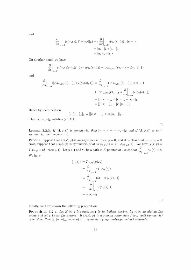
and

∂

∂s

∣∣∣∣s=0

(ǫ(γu(s), 1) [v, 0]L) = (∂

∂s

∣∣∣∣s=0

ǫ(γu(s), 1)) [v,−]L

= [u,−]L [v,−]L

= [u, [v,−]L]L.

On another hand, we have

∂

∂t

∣∣∣∣t=0

(ǫ(γu(s)⊲γv(t), 1) ǫ(γu(s), 1)) = [Adγu(s)(v),−]L ǫ(γu(s), 1)

and

∂

∂s

∣∣∣∣s=0

([Adγu(s)(v),−]L ǫ(γu(s), 1)) =∂

∂s

∣∣∣∣s=0

([Adγu(s)(v),−]L) ǫ(1, 1)

+ [Adγu(0)(v),−]L ∂

∂s

∣∣∣∣s=0

(ǫ(γu(s), 1))

= [[u, v],−]L + [v,−]L [u,−]L

= [[u, v],−]L + [v, [u,−]]L.

Hence by identification[u, [v,−]L]L = [[u, v],−]L + [v, [u,−]]L.

That is, [−,−]L satisfies (LLM).

Lemma 3.2.3. If (A, φ, ψ) is symmetric, then [−,−]L = −[−,−]R and if (A, φ, ψ) is anti-symmetric, then [−,−]R = 0.

Proof : Suppose that (A, φ, ψ) is anti-symmetric, then ψ = 0, and it is clear that [−,−]R = 0.Now, suppose that (A, φ, ψ) is symmetric, that is ψx,y(a) = a − φx⊲y,1(a). We have χ(x, y) =

T1ψx,y = id−ǫ(x⊲y, 1). Let u ∈ x and γu be a path in X pointed at 1 such that∂

∂s

∣∣∣∣s=0

γu(s) = u.

We have

[−, u]R = T(1,1)χ(0, u)

=∂

∂s

∣∣∣∣s=0

χ(1, γu(s))

=∂

∂s

∣∣∣∣s=0

(id− ǫ(γu(s), 1))

= −∂

∂s

∣∣∣∣s=0

ǫ(γu(s), 1)

= −[u,−]L.

Finally, we have shown the following proposition:

Proposition 3.2.4. Let X be a Lie rack, let x be its Leibniz algebra, let A be an abelian Liegroup and let a be its Lie algebra. If (A, φ, ψ) is a smooth symmetric (resp. anti-symmetric)X-module, then (a, [−,−]L, [−,−]R) is a symmetric (resp. anti-symmetric) x-module.

55

3.3 From Lie rack cohomology to Leibniz cohomology

3.3.1 A morphism from Lie rack cohomology to Leibniz cohomology

Proposition 3.3.1. Let X be a Lie rack and let A be a smooth As(X)-module. We havemorphisms of cochains complexes

CRnp (X,As)s

δn

→ CLn(x, as)

andCRn

p (X,Aa)sδn

→ CLn(x, aa),

given by δn(f)(a1, . . . , an) = dnf(1, . . . , 1)((a1, 0, . . . , 0), . . . , (0, . . . , 0, an)) (where dnf is the n-thdifferential of f).

Proof : Let f ∈ CRnp (X,As) and (x0, . . . , xn) ∈ Xn+1. We have

dRf(x0, . . . , xn) =

n+1∑

i=1

(−1)i−1φx1⊲...⊲xi(f(x1, . . . , xi, . . . , xn+1))−f(x1, . . . , xi⊲xi+1, . . . , xi⊲xn+1)

(Here φx1⊲...⊲xi= φx1⊲...⊲xi,x1⊲...⊲cx1⊲...⊲xn+1

cf. section 3.2)Let (γ0(t0), . . . , γn(tn)) be a family of paths γi :] − ǫi,+ǫi[→ V such that

γi(0) = 1 and∂

∂s s=0γi(s) = xi.

We want to show thatδn+1(dn

Rf) = dnL(δn(f)).

We have by definition

δn+1(dnRf)(a0, . . . , an) =

∂n+1

∂t0 . . . ∂tn

∣∣∣∣ti=0

df(γ0(t0), . . . , γn(tn)).

Lemma 3.3.2. ∀i ∈ 1, . . . , n

∂n+1

∂t0 . . . ∂tn

∣∣∣∣|ti=0

φγ0(t0)⊲...⊲γi(ti)(f(γ0(t0), . . . , γi−1(ti−1), γi+1(ti+1), . . . , γn(tn))) = ai.dn(f)(a0, . . . , ai, . . . , an)

Proof :Notation:

(t0, . . . , ti) 7→ φγ0(t0)⊲...⊲γi(ti)

will be denoted by(t0, . . . , ti) 7→ A(t0, . . . , ti)

and(t0, . . . , ti, . . . , tn) 7→ f(γ0(t0), . . . , γi−1(ti−1), γi+1(ti+1), . . . , γn(tn))

will be denoted by(t0, . . . , ti, . . . , tn) 7→ m(t0, . . . , ti, . . . , tn)

56

We have

∂n+1

∂t0 . . . ∂tn

∣∣∣∣tk=0

A(t0, . . . , ti)(m(t0, . . . , tn)) =∂n

∂t0 . . . ∂tn−1

∣∣∣∣tk=0

(∂

∂tn tn=0

A(t0, . . . , ti)(m(t0, . . . , 0))

+∂n

∂t0 . . . ∂tn−1

∣∣∣∣tk=0

(A(t0, . . . , ti)(∂

∂tn

∣∣∣∣tn=0

m(t0, . . . , tn)))

=∂n

∂t0 . . . ∂tn−1

∣∣∣∣tk=0

(A(t0, . . . , ti)(∂

∂tn tn=0

m(t0, . . . , tn)))

because f(x0, . . . , 1, . . . , xn) = 0 (cf. Definition 2.3.11).So by the same argument we have

∂n+1

∂t0 . . . ∂tn

∣∣∣∣tk=0

A(t0, . . . , ti)(m(t0, . . . , tn)) =∂

∂ti

∣∣∣∣ti=0

A(0, . . . , 0, ti)(∂n

∂t0 . . . ∂tn

∣∣∣∣tk=0

m(t0, . . . , tn))

Hence∂n+1

∂t0 . . . ∂tn

∣∣∣∣ti=0

A(t0, . . . , tn)(m(t0, . . . , tn)) = xi.dn(f)(x0, . . . , xi, . . . , xn)

Lemma 3.3.3. ∀i ∈ 1, . . . , n

∂n+1

∂t0 . . . ∂tn

∣∣∣∣ti=0

f(γ0(t0), . . . , γi(ti)⊲γi+1(ti+1), . . . , γi(ti)⊲γn(tn)) =n∑

k=i+1

δnf(a0, . . . , [ai, ak], . . . , an)

Proof : We have∂n+1

∂t0 . . . ∂tn

∣∣∣∣ti=0

f(γ0(t0), . . . , γi(ti)⊲γi+1(ti+1), . . . , γi(ti)⊲γn(tn)) which is

equal to

∂

∂ti

∣∣∣∣ti=0

dnf(1, . . . , 1)((a0, 0, . . . , 0), . . . , (0, . . . , Adγi(ti)(ai+1), . . . , 0), . . . , (0, . . . , 0, Adγi(ti)(an))

Moreover, this is equal to

n∑

k=i+1

dnf(1, . . . , 1)((a0, 0, . . . , 0), . . . , (0, . . . , [ai, ak], . . . , 0), . . . , (0, . . . , 0, an))

and this expression is equal ton∑

k=i+1

δnf(a0, . . . , [ai, ak], . . . , an).

So

δn+1(dnRf)(a0, . . . , an) =

n∑

i=0

(−1)i(ai.δ

n(f)(a0, . . . , ai, . . . , an) −n∑

k=i+1

δnf(a0, . . . , [ai, ak], . . . , an))

=

n∑

i=0

(−1)iai.δn(f)(a0, . . . , ai, . . . , an) +

∑

0≤i<k≤n

(−1)i+1δnf(a0, . . . , [ai, ak], . . . , an)

that isδn+1(dn

Rf) = dnL(δn(f))

This is exactly the same proof as for the case where A is anti-symmetric.

57

We remark that we only need a local cocyle identity around 1. Thus we have

Proposition 3.3.4. Let X be a Lie rack, let U be a 1-neighborhood in X and let A be a smoothAs(X)-module. We have morphisms of cochain complexes

CRnp (U,As)

δn

→ CLn(x, as)

andCRn

p (U,Aa)δn

→ CLn(x, aa),

given by δn(f)(a0, . . . , an) = dnf(1, . . . , 1)((a1, 0, . . . , 0), . . . , (0, . . . , 0, an)).

3.3.2 Induced morphism from Lie cohomology to Leibniz cohomology

Let G be a Lie group and A a smooth G-module. We have stated in Proposition 2.3.24 that

there are maps Hn(G,A)∆n

→ HRn(G,As) for all n ∈ N. These maps still exist when the cocycles

are smooth, that is we have maps Hn(G,A)s∆n

→ HRn(G,As)s for all n ∈ N. On the other hand,

we have shown that for g a Lie algebra and a a g-module, there are maps Hn(g, a)in→ HLn(g, as)

for all n ∈ N. K.H. Neeb defines in [Nee04], maps Hn(G,A)sDn

→ Hn(g, a) for all n ∈ N, and we

have defined maps HRn(G,As)δn

→ HLn(g, as) for all n ∈ N. It is natural to believe that there isa link between those maps. The Proposition 3.3.6 confirms this belief.

First of all, recall the maps Dnn∈N defined in [Nee04] (Theorem B.6).

Proposition 3.3.5 (Van Est). Let G be a Lie group and let A be a smooth G-module. We havemorphisms of cochain complexes

Cns (G,A)

Dn

→ Cn(g, a)

given by Dn(f)(a1, . . . , an) =∑

σ∈σn

(−1)sign(σ)dnf(1, . . . , 1)((aσ(1), 0, . . . , 0), . . . , (0, . . . , 0, aσ(n))).

Proof : It is the content of Theorem B.6 in [Nee04].

Proposition 3.3.6. Let G be a Lie group and let A be a smooth G-module. The diagram

Cn(G,A)s, dnn∈N

∆nn∈N //

Dnn∈N

CRnp (G,As)s, d

nRn∈N

δnn∈N

Cn(g, a), dnn∈N

inn∈N

// CLn(g, as), dnLn∈N

is a commutative diagram of morphisms of cochain complexes.

To prove this result, we need the following lemma.

58

Lemma 3.3.7. Let 1 ≤ k ≤ n, f ∈ Cn(G,A)s, (g1, . . . , gn) ∈ Gn and (v1, . . . , vk) ∈ (gn)k suchthat

gi1 = · · · = gik+1= 1

for 1 ≤ i1 < · · · < ik+1 ≤ n, and

vj = (0, . . . , 0, xij, 0, . . . , 0)

for xij∈ g.

We havedkf(g1, . . . , gn)(v1, . . . , vk) = 0.

Proof : Let γijbe a path in G such that γij

(0) = 1 and∂

∂t

∣∣∣∣t=0

γij(t) = xij

. We have f ∈

Cn(G,A)s, thusf(g1, . . . , γi1(t1), . . . , γik

(tk), . . . , 1, . . . , gn) = 0.

Moreover, we have

∂k

∂t1 . . . ∂tk

∣∣∣∣t1...tk=0

f(g1, . . . , γi1(t1), . . . , γik(tk), . . . , 1, . . . , gn) = dkf(g1, . . . , gn)(v1, . . . , vk).

Hence,dkf(g1, . . . , gn)(v1, . . . , vk) = 0.

Proof of the Proposition : We have to show that for all n ∈ N,

δn ∆n = in Dn.

Let f ∈ Cn(G,A), x1, . . . , xn ∈ g and γ1, . . . , γn paths inG, such that γi(0) = 1 and∂

∂t

∣∣∣∣t=0

γi(t) =

xi. We have

δn(∆n(f))(x1, . . . , xn) =∂n

∂t1 . . . ∂tn

∣∣∣∣t1...tn=0

∆n(f)(γ1(t1), . . . , γn(tn))

=∑

σ∈Sn

(−1)sign(σ) ∂n

∂t1 . . . ∂tn

∣∣∣∣t1...tn=0

f(γσ1 (t1, . . . , tn), . . . , γσ

n(t1, . . . , tn))

whereγσ

k (t1, . . . , tn) = γj1(tj1)⊲ . . .⊲γjl(tjl

)⊲γσ(k)(tσ(k))

with j1 < · · · < jl < σ(k) and ji /∈ σ(1), . . . , σ(k).

Let 1 ≤ k ≤ n, suppose that the following formula is true

∂n−k+1

∂tk . . . ∂tn

∣∣∣∣tk...tn=0

f(γσ1 (t1, . . . , tn), . . . , γσ

n(t1, . . . , tn)) = dn−k+1f(g1, . . . , gn)(v1, . . . , vn−k+1)

where

gi =

1 if i ∈ σ−1(k), . . . , σ−1(n)γσ

i (t1, . . . , tk) else if

59

and vi = (v1i , . . . , v

ni ) with

vji =

0 if j 6= σ−1(k − 1 + i)∂

∂tj

∣∣∣∣tj=0

γσσ−1(j)(t1, . . . , tk−1, 1, . . . , 1, tj) else if

We have

∂n−k+2

∂tk−1 . . . ∂tn

∣∣∣∣tk−1...tn=0

f(γσ1 (t1, . . . , tn), . . . , γσ

n(t1, . . . , tn)) =∂

∂tk−1

∣∣∣∣tk−1=0

(dn−k+1f(g1, . . . , gn)(v1, . . . , vn−k+1))

and

∂

∂tk−1

∣∣∣∣tk−1=0

(dn−k+1f(g1, . . . , gn)(v1, . . . , vn−k+1)) = dn−k+2f(h1, . . . , hn)(w1, . . . , wn−k+2)

+k∑

i=1

dn−k+1f(h1, . . . , hn)(v1(t1, . . . , tk−2, 1), . . . ,∂

∂tk−1

∣∣∣∣tk−1=0

vi(t1, . . . , tk−1), . . . , vk(t1, . . . , tk−2, 1))

where

hi =

1 if i ∈ σ−1(k − 1), . . . , σ−1(n)γσ

i (t1, . . . , tk−1) else if

and w1 = (w11, . . . , w

n1 ) with

wj1 =

0 if j 6= σ−1(k − 1)∂

∂tk−1

∣∣∣∣tk−1=0

γσσ−1(k−1)(t1, . . . , tk−1) else if

and wji (t1, . . . , tk−2) = vj

i−1(t1, . . . , tk−2, 1).

By Lemma 3.3.7, the term

k∑

i=1

dn−k+1f(h1, . . . , hn)(v1(t1, . . . , tk−2, 1), . . . ,∂

∂tk−1

∣∣∣∣tk−1=0

vi(t1, . . . , tk−1), . . . , vk(t1, . . . , tk−2, 1))

is equal to zero. Thus, if the formula (3.3.2) is true, then we have

∂n−k+2

∂tk−1 . . . ∂tn

∣∣∣∣tk−1...tn=0

f(γσ1 (t1, . . . , tn), . . . , γσ

n(t1, . . . , tn)) = dn−k+2f(g1, . . . , gn)(v1, . . . , vn−k+1).

As this formula is true for k = n, by induction this formula is true for k = 1. That is,

∂n

∂t1 . . . ∂tn

∣∣∣∣t1...tn=0

f(γσ1 (t1, . . . , tn), . . . , γσ

n(t1, . . . , tn)) = dnf(g1, . . . , gn)(v1, . . . , vn).

Hence,

δn(∆n(f))(x1, . . . , xn) =∑

σ∈Sn

(−1)sign(σ)dnf(1, . . . , 1)(v1, . . . , vn)

= in(Dn(f))(x1, . . . , xn).

Thusδn ∆n = in Dn.

60

Hence we have for all n ∈ N a commutative diagram

Hn(G,A)s

[∆n] //

[Dn]

HRns (G,As)

[δn]

Hn(g, a)

[in]// HLn(g, as)

In [Nee04], K.H. Neeb shows in particular that, if the Lie group G is simply connected, thenD2 is an isomorphism and its inverse is given by

ι2(ω)(g, h) =

∫

γg,h

ωeq

where γg,h is a smooth singular 2-chain in G such that ∂γg,h = γg − γgh + gγh and γg (resp. γh)a smooth path in G from 1 to g (resp. h).

3.4 From Leibniz cohomology to Lie local rack cohomology

In this section, we study two cases of Leibniz cocyles integration. This section will be used inthe following section to integrate a Leibniz algebra into a local augmented Lie rack.First, we study the integration of a 1-cocycle in ZL1(g, as) into a Lie rack 1-cocycle in ZR1

p(G, as)s,

where G is a simply connected Lie group with Lie algebra g and a a representation of G.Secondly, we use the result of the first part to study the integration of a 2-cocycle in ZL2(g, aa)into a local Lie rack 2-cocycle in ZR2

p(U, aa)s, where U is a 1-neighborhood in a simply connected

Lie group G with Lie algebra g, and a a representation of G. It is this second part that we willuse to integrate Leibniz algebras.

3.4.1 From Leibniz 1-cocycles to Lie rack 1-cocycles

Let G be a simply connected Lie group and a a representation of G. We want to define amorphism I1 from ZL1(g, as) to ZR1

p(G, as)s which sends BL1(g, as) into BR1

p(G, as)s. For this,

we put

I1(ω)(g) =

∫

γg

ωeq,

where ω ∈ ZL1(g, as), γ : G× [0, 1] → G is a smooth map such that γg is a path from 1 to g, γ1

is the constant path equal to 1, and ωeq is the closed left equivariant differential form in Ω1(G, a)defined by

ωeq(g)(m) = g.(ω(TgLg−1(m))).

By definition, it is clear that I1(ω)(1) = 0.For the moment, I1(ω) depends on γ, but because ω is a cocycle, the dependance with respect

to γ disappears.

Proposition 3.4.1. I1 does not depend on γ.

61

Proof : Let γ, γ′ : G × [0, 1] → G such that γg(0) = γ′g(0) = 1 and γg(1) = γ′g(1) = g. We aregoing to show that

∫

γg

ωeq =

∫

γ′g

ωeq.

We have∫

γgωeq −

∫γ′

gωeq =

∫γg−γ′

gωeq. As H1(G) = 0 and ∂(γg − γ′g) = 0, there exists

σg : [0, 1]2 → G such that γg − γ′g = ∂σg. So

∫

γg

ωeq −

∫

γ′g

ωeq =

∫

γg−γ′g

ωeq

=

∫

∂σg

ωeq

=

∫

σg

ddRωeq

= 0.

Hence I1 does not depend on γ.

Proposition 3.4.2. I1 sends cocycles to cocycles and coboundaries to coboundaries.

Proof : First, let ω ∈ ZL1(g, as), we have

dRI(ω)(g, h) = g.I(ω)(h) − I(ω)(g⊲h) − (g⊲h).I(ω)(g) + I(ω)(g)

= g.

∫

γh

ωeq −

∫

γg⊲h

ωeq − (g⊲h).

∫

γg

ωeq +

∫

γg

ωeq

=

∫

γh

g.ωeq −

∫

γg⊲h

ωeq −

∫

γg

(g⊲h).ωeq +

∫

γg

ωeq

=

∫

gγh

ωeq −

∫

γg⊲h

ωeq −

∫

(g⊲h)γg

ωeq +

∫

γg

ωeq

=

∫

gγh−γg⊲h−(g⊲h)γg+γg

ωeq.

As H1(G) = 0 and ∂(gγh − γg⊲h − (g⊲h)γg + γg) = 0, there exists γg,h : [0, 1]2 → G such that∂γg,h = gγh − γg⊲h − (g⊲h)γg + γg. Hence, we have

dRI(ω)(g, h) =

∫

∂γg,h

ωeq

=

∫

γg,h

ddRωeq

= 0.

Hence ZL1(g, as) is sent to ZR1p(G, a

s)s.

62

Secondly, let ω ∈ BL1(g, as). There exists β ∈ a such that ω(m) = m.β. We have

I(ω)(g) =

∫

γg

ωeq

=

∫

γg

(dLβ)eq

=

∫

γg

ddRβeq

= βeq(g) − βeq(1)

= g.β − β

= dRβ(g).

Hence BL1(g, as) is sent to BR1p(G, a

s)s.

Proposition 3.4.3. I1 is a left inverse for δ1.

Proof : Let ω ∈ ZL1(g, as). Let ϕ : U → g be a local chart around 1 such that ϕ(1) = 0 anddϕ−1(0) = id.We define for x ∈ g the smooth map αx :] − ǫ,+ǫ[→ U by setting

αx(s) = ϕ−1(sx),

and we define for all s ∈] − ǫ,+ǫ[, the smooth map γαx(s) : [0, 1] → U by setting

γαx(s)(t) = ϕ−1(tsx).

We have

δ1(I1(ω))(x) =∂

∂s

∣∣∣∣s=0

I1(ω)(αx(s))

=∂

∂s

∣∣∣∣s=0

∫

γαx(s)

ωeq

=∂

∂s

∣∣∣∣s=0

∫

[0,1]

γ∗αx(s)ωeq

=∂

∂s

∣∣∣∣s=0

∫

[0,1]

ωeq(γαx(s)(t))(∂

∂t

∣∣∣∣t=0

γαx(s)(t))dt.

63

Moreover,∂

∂t

∣∣∣∣t=0

γαx(s)(t) =∂

∂t

∣∣∣∣t=0

ϕ−1(stx) = sx, thus

δ1(I1(ω))(x) =∂

∂s

∣∣∣∣s=0

∫

[0,1]

ωeq(γαx(s)(t))(sx)dt

=

∫

[0,1]

∂

∂s

∣∣∣∣s=0

ωeq(γαx(s)(t))(sx)dt

=

∫

[0,1]

∂

∂s

∣∣∣∣s=0

ωeq(ϕ−1(tsx))(sx)dt

=

∫

[0,1]

∂

∂s

∣∣∣∣s=0

(ϕ−1)∗ωeq(tsx)(sx)dt

=

∫

[0,1]

∂

∂s

∣∣∣∣s=0

s(ϕ−1)∗ωeq(tsx)(x)dt

=

∫

[0,1]

(ϕ−1)∗ωeq(0)(x)dt

= ω(x)

∫

[0,1]

dt

= ω(x).

Hence δ1 I1 = id.

Remark 3.4.4. The morphism H1(g, a)D1

→ H1s (G, a) is an isomorphism (cf. for example

[Nee04]). We can remark that I1 is the same map as the one defined in [Nee04] to provethe surjectivity. In fact, to prove the Proposition 3.4.2, we just compose the map D1 and themap ∆1 defined in Proposition 2.3.24 (Precisely, we use the remark below this proposition which

states that H1s (G, a)s

∆1

→ HR1s(G, a

s) is an injection).

3.4.2 From Leibniz 2-cocycles to Lie local rack 2-cocycles

Let G be a simply connected Lie group, let U be a 1-neigbourhood in G such that log is definedon U and let a be a representation of G. In Proposition 3.3.4 we have defined for all n ∈ N themaps

HRns (U, aa)

[δn]−→ HLn(g, aa).

In the next section, we will see that a Leibniz algebra can be integrated into a local Lie racksince the morphism [δ2] is surjective. More precisely, if we can construct a left inverse for [δ2],then it gives us an explicit method to construct the local Lie rack which integrates the Leibnizalgebra.

In this section, we define a morphism [I2] from HL2(g, aa) to HR2s(U, a

a), and we show thatit is a left inverse for [δ2]. To construct the map [I2], we adapt an integration method of Liealgebra cocycles into Lie group cocycles by integration over simplex. This method is due to W.T.Van Est ([Est54]) and used by K.H. Neeb ([Nee02, Nee04]) for the infinite dimensional case.

64

Definition of I2

We want to define a map from ZL2(g, aa) to ZR2p(U, a

a)s such that BL2(g, aa) is sent toBR2

p(U, aa)s. In the previous section, we have integrated a Leibniz 1-cocycle on a Lie alge-

bra g with coefficients in a symmetric module as. In Proposition 1.3.16, we have shown thatthere is an isomorphism between CL2(g, aa) and CL1(g, Hom(g, a)s), which sends ZL2(g, aa) toZL1(g, Hom(g, a)s) and BL2(g, aa) to BL1(g, Hom(g, a)s). Hence, we can define a map

I : ZL2(g, aa) → ZR1p(G,Hom(g, a)s)s,

which sends BL2(g, aa) into BR1p(G,Hom(g, a)s)s. This is the composition

ZL2(g, aa)τ2

→ ZL1(g, Hom(g, a)s)I1

→ ZR1p(G,Hom(g, a)s)s.

Now, we want to define a map from ZR1p(G,Hom(g, a)s)s to ZR2

p(U, aa). Let β ∈ CR1

p(G,Hom(g, a)s)s,β has values in the representation Hom(g, a), so for all g ∈ G, we can consider the equivariantdifferential form β(g)eq ∈ Ω1(G, a) defined by

β(g)eq(h)(m) := h.(β(g)(ThLh−1(m))).

Then we define an element in CR2p(U, a

a) by setting

f(g, h) =

∫

γg⊲h

(β(g))eq,

where γ : G× [0, 1] → G is a smooth map such that for all g ∈ G, γg is a path from 1 to g in Gand γ1 = 1.For the moment, an element of ZR1

p(G,Hom(g, a)s)s is not necessarily sent to an element ofZR2

p(U, aa)s. To reach our objective, we have to specify the map γ, and we define it by setting

γg(s) = exp(s log(g)).

Then, we define I2 : ZL2(g, aa) → CR2p(U, a

a)s by setting for all (g, h) ∈ U2−loc

I2(ω)(g, h) =

∫

γg⊲h

(I(ω)(g))eq.

By definition, it is clear that I2(ω)(g, 1) = I2(ω)(1, g) = 0.

Properties of I2

Proposition 3.4.5. I2 sends ZL2(g, aa) into ZR2p(U, a

a)s.

To prove this proposition we need some lemmas.

Lemma 3.4.6. For all (g, h) ∈ U2−loc, we have γg⊲h = g⊲γh.

Proof : Let (g, h) ∈ U2−loc, by definition we have

γg⊲h(s) = exp(s(log(g⊲h))).

By naturality of the exponential, and a fortiori of the logarithm, we have

exp(s(log(g⊲h))) = exp(sAdg(log(h)))

= exp(Adg(s log(h)))

= cg(exp(s log(h)))

= cg(γh(s)).

Hence γg⊲h = g⊲γh.

65

Lemma 3.4.7. Let G be a Lie group, let a be a representation of G and ω ∈ Hom(g, a). Wehave for all g ∈ G

g.(ωeq) = c∗g((g.ω)eq).

Proof : Let g, h ∈ G and x ∈ ThG, we have:

(c∗g((g.ω)eq))(h)(x) = (g.ω)eq(g⊲h)(dhcg(x))

= (g⊲h).(g.ω)(dg⊲hLg⊲h−1(dhcg(x)))

= (g⊲h).(g.ω)(dh(cg Lh−1)(x))

= (g⊲h).(g.(ω(Ad(g−1)(dh(cg Lh−1)(x)))))

= gh.(ω(dh(cg−1 cg Lh−1)(x)))

= g.(h.(ω(dhLh−1(x))))

= g.(ωeq(h)(x)).

Hence c∗g((g.ω)eq) = g.(ω)eq.

Proof of proposition : Let ω ∈ ZL2(g, aa) and (g, h, k) ∈ U3−loc. We have

dR(I2(ω))(g, h, k) = g.I2(ω)(h, k) − I2(ω)(g⊲h, g⊲k) − (g⊲h).I2(ω)(g, k) + I2(ω)(g, h⊲k)

= g.

∫

γh⊲k

(I(ω)(h))eq −

∫

γg⊲(h⊲k)

(I(ω)(g⊲h))eq − (g⊲h).

∫

γg⊲k

(I(ω)(g))eq

+

∫

γg⊲(h⊲k)

(I(ω)(g))eq

=

∫

γh⊲k

g.((I(ω)(h))eq) −

∫

γg⊲(h⊲k)

(I(ω)(g⊲h))eq −

∫

γg⊲k

(g⊲h).((I(ω)(g))eq)

+

∫

γg⊲(h⊲k)

(I(ω)(g))eq.

Because of Lemma 3.4.7, we have

dR(I2(ω))(g, h, k) =

∫

γh⊲k

c∗g((g.I(ω)(h))eq) −

∫

γg⊲(h⊲k)

I(ω)(g⊲h)eq −

∫

γg⊲k

c∗g⊲h(((g⊲h).I(ω)(g))eq)

+

∫

γg⊲(h⊲k)

I(ω)(g)eq

=

∫

cgγh⊲k

(g.I(ω)(h)eq −

∫

γg⊲(h⊲k)

I(ω)(g⊲h)eq −

∫

cg⊲hγg⊲k

((g⊲h).I(ω)(g))eq

+

∫

γg⊲(h⊲k)

I(ω)(g)eq,

66

and because of Lemma 3.4.6, we have

dR(I2(ω))(g, h, k) =

∫

γg⊲(h⊲k)

(g.I(ω)(h))eq −

∫

γg⊲(h⊲k)

I(ω)(g⊲h)eq −

∫

γg⊲(h⊲k

((g⊲h).I(ω)(g))eq

+

∫

γg⊲(h⊲k)

I(ω)(g)eq

=

∫

γg⊲(h⊲k)

(g.I(ω)(h))eq − I(ω)(g⊲h)eq − ((g⊲h).I(ω)(g))eq + I(ω)(g)eq

=

∫

γg⊲(h⊲k)

(g.I(ω)(h) − I(ω((g⊲h) − (g⊲h).I(ω)(g) + I(ω)(g))eq

=

∫

γg⊲(h⊲k)

dR(I(ω))(g, h)

= 0.

Hence ZL2(g, aa) is sent to ZR2p(U, a

a)s.

Proposition 3.4.8. I2 sends BL2(g, aa) into BR2p(U, a

a)s.

Proof : Let ω ∈ BL2(g, aa), there exists an element β ∈ CL1(g, aa) such that ω = dLβ. Wehave

I(ω)(g) = I1(τ2(ω))(g)

=

∫

γg

(τ2(ω))eq

=

∫

γg

(τ2(dLβ))eq.

The fact that τnn∈N is a morphism of cochain complexes implies that

I(ω)(g) =

∫

γg

(d(τ1(β)))eq

=

∫

γg

ddR((τ1(β))eq)

=

∫

∂γg

(τ1(β))eq

= g.β − β.

67

Hence for (g, h) ∈ U2−loc we have using Lemma 3.4.7

I2(ω)(g, h) =

∫

γg⊲h

(I(ω)(g))eq

=

∫

γg⊲h

((g.β) − β)eq

=

∫

γg⊲h

(g.β)eq −

∫

γg⊲h

βeq

=

∫

γg⊲h

(c∗g−1(g.(βeq))) −

∫

γg⊲h

βeq

=

∫

cg−1γg⊲h

g.(βeq) −

∫

γg⊲h

βeq

= g.

∫

cg−1γg⊲h

βeq −

∫

γg⊲h

βeq

= g.

∫

γh

βeq −

∫

γg⊲h

βeq

= dR(I1(β))(g, h).

Hence BL2(g, aa) is sent to BR2p(U, a)s.

Proposition 3.4.9. I2 is a left inverse for δ2.

Proof : Let x, y ∈ g, and Ix (resp Iy) be an interval in R such that ǫx(s) = exp(sx) (respǫy(s) = exp(sy)) be defined for all s ∈ Ix (resp for all s ∈ Iy). The map ǫx⊲ǫy : Ix × Iy → G iscontinuous, thus there exists W an open subset of Ix × Iy such that (ǫx⊲ǫy)(W ) ⊆ U . Hence,there exists an interval J ⊆ Ix ∩ Iy such that ǫx(s)⊲ǫy(t) ∈ U for all (s, t) ∈ J × J .

We have to showδ2 I2 = id.

Let ω ∈ ZL2(g, aa). By definition, we have

δ2(I2(ω))(x, y) =∂2

∂s∂t

∣∣∣∣|s,t=0

I2(ω)(ǫx(s), ǫy(s))

=∂2

∂s∂t

∣∣∣∣|s,t=0

∫

γǫx(s)⊲ǫy(t)

(I(ω)(ǫx(s)))eq

=∂

∂s

∣∣∣∣|s=0

(∂

∂t

∣∣∣∣|t=0

∫

γǫy(t)

c∗ǫx(s)(I(ω)(ǫx(s)))eq).

First, we compute∂

∂t

∣∣∣∣|t=0

∫

γǫy(t)

c∗ǫx(s)(I(ω)(ǫx(s)))eq

68

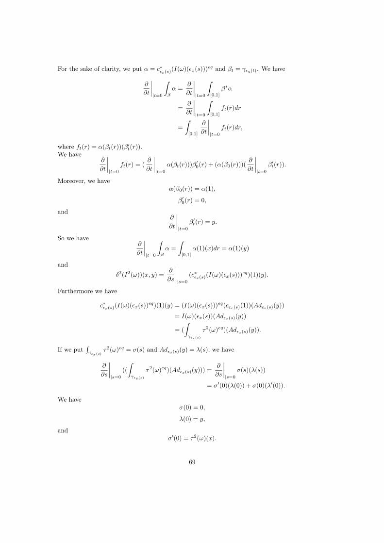
For the sake of clarity, we put α = c∗ǫx(s)(I(ω)(ǫx(s)))eq and βt = γǫy(t). We have

∂

∂t

∣∣∣∣|t=0

∫

β

α =∂

∂t

∣∣∣∣|t=0

∫

[0,1]

β∗α

=∂

∂t

∣∣∣∣|t=0

∫

[0,1]

ft(r)dr

=

∫

[0,1]

∂

∂t

∣∣∣∣|t=0

ft(r)dr,

where ft(r) = α(βt(r))(β′t(r)).

We have∂

∂t

∣∣∣∣|t=0

ft(r) = (∂

∂t

∣∣∣∣|t=0

α(βt(r)))β′0(r) + (α(β0(r)))(

∂

∂t

∣∣∣∣|t=0

β′t(r)).

Moreover, we haveα(β0(r)) = α(1),

β′0(r) = 0,

and∂

∂t

∣∣∣∣|t=0

β′t(r) = y.

So we have∂

∂t

∣∣∣∣|t=0

∫

β

α =

∫

[0,1]

α(1)(x)dr = α(1)(y)

and

δ2(I2(ω))(x, y) =∂

∂s

∣∣∣∣|s=0

(c∗ǫx(s)(I(ω)(ǫx(s)))eq)(1)(y).

Furthermore we have

c∗ǫx(s)(I(ω)(ǫx(s))eq)(1)(y) = (I(ω)(ǫx(s)))eq(cǫx(s)(1))(Adǫx(s)(y))

= I(ω)(ǫx(s))(Adǫx(s)(y))

= (

∫

γǫx(s)

τ2(ω)eq)(Adǫx(s)(y)).

If we put∫

γǫx(s)τ2(ω)eq = σ(s) and Adǫx(s)(y) = λ(s), we have

∂

∂s

∣∣∣∣|s=0

((

∫

γǫx(s)

τ2(ω)eq)(Adǫx(s)(y))) =∂

∂s

∣∣∣∣|s=0

σ(s)(λ(s))

= σ′(0)(λ(0)) + σ(0)(λ′(0)).

We haveσ(0) = 0,

λ(0) = y,

andσ′(0) = τ2(ω)(x).

69

Thus∂

∂s

∣∣∣∣|s=0

((

∫

γǫx(s)

τ2(ω)eq)(Adǫx(s)(y))) = τ2(ω)(x)(y).

Hence δ2(I2(ω))(x, y) = ω(x, y).

Remark 3.4.10. Suppose that we have a Leibniz 2-cocycle ω which is also a Lie 2-cocycle. Inthis case, we can integrate ω into a local Lie rack cocycle, but also into a local Lie group cocycle.Then it is natural to ask if the two constructions are related to each other.

Proposition 3.4.11. Let G be a Lie group, let g be its Lie algebra, let a be a representation ofG, ω ∈ Λ2(g, a) and γ1, γ2 smooth paths in G pointed in 1. Then

∫

γ1

( ∫

γ2

(τ2(ω))eq)eq

=

∫

γ1γ2

ωeq

where γ1γ2 : [0, 1]2 → G; (s, t) 7→ γ1(t)γ2(s).

Proof : On the hand, we have∫

γ1γ2

ωeq =

∫

[0,1]2(γ1γ2)

∗ωeq

=

∫

[0,1]2ωeq(γ1γ2)(

∂

∂sγ1(t)γ2(s),

∂

∂tγ1(t)γ2(s))dsdt,

and this expression is equal to∫

[0,1]2γ1(t)γ2(s).ω

(dγ2(s)Lγ2(s)−1(

∂

∂sγ2(s)), Adγ2(s)−1(dγ1(t)Lγ1(t)−1(

∂

∂tγ1(t)))

). (3.1)

On the other hand, we have∫

γ1

( ∫

γ2

(τ2(ω))eq)eq

=

∫

[0,1]

γ∗1 (

∫

γ2

(τ2(ω)eq)eq)

=

∫

[0,1]

(

∫

γ2

(τ2(ω))eq)eq(γ1(t))(∂

∂tγ1(t))dt

=

∫

[0,1]

γ1(t).(

∫

γ2

(τ2(ω))eq)(dγ1(t)Lγ1(t)−1(∂

∂tγ1(t)))dt

=

∫

[0,1]

γ1(t).(

∫

[0,1]

(τ2(ω))eq(γ2(s))(∂

∂sγ2(s)))(dγ1(t)Lγ1(t)−1(

∂

∂tγ1(t)))dt.

This expression is equal to∫

[0,1]

γ1(t).(

∫

[0,1]

γ2(s).(τ2(ω))(dγ2(s)Lγ2(s)−1(

∂

∂sγ2(s)))ds)(dγ1(t)Lγ1(t)−1(

∂

∂tγ1(t)))dt,

which is equal to∫

[0,1]

γ1(t).(

∫

[0,1]

γ2(s).ω(dγ2(s)Lγ2(s)−1(∂

∂sγ2(s)), Adγ2(s)−1(·))ds)(dγ1(t)Lγ1(t)−1(

∂

∂tγ1(t)))dt.

Using the Fubini theorem, we show that this expression is equal to (3.1).

70

If we apply this result to the case where γ1(s) = γg⊲h(s) = exp(s log(g⊲h)) and γ2(s) = γg(s) =exp(s log(g)) for (g, h) ∈ U2−loc, then we obtain

Corollary 3.4.12. If ω ∈ ZL2(g, aa) ∩ Z2(g, a), then I2(ω) = ∆2(ι2(ω)).

We can remark that I2 is more than a local Lie rack cocycle. Precisely, if ω is in ZL2(g, aa)then the local rack cocycle identity satisfied by I2(ω), comes from another identity satisfied byI2(ω). Indeed, I2 is defined using I, and to verify that I2 sends Leibniz cocycles into local rackcocycles, we have used Proposition 3.4.2. This proposition establishes that I1 sends Lie cocyclesinto rack cocycle. But, we have remarked in Proposition 3.4.4 that the rack cocycle identitysatisfied by I1(ω), comes from the group cocycle identity. Hence, we can think that we forgotstructure on I2(ω). The following proposition identifies the identity satisfied by I2(ω) whichinduced the local rack identity.

Proposition 3.4.13. If ω ∈ ZL2(g, aa), then I2(ω) satisfies the identity

g.I2(ω)(h, k) − I2(ω)(gh, k) + I2(ω)(g, h⊲k) = 0, ∀(g, h, k) ∈ U3−loc.

Moreover, this identity induces the local rack cocycle identity.

Proof : Let ω ∈ ZL2(g, aa) and (g, h, k) ∈ U3−loc we have:

g.I2(ω)(h, k) − I2(ω)(gh, k) + I2(ω)(g, h⊲k) = g.

∫

γh⊲k

(I(ω)(h))eq −

∫

γ(gh)⊲k

(I(ω)(gh))eq

+

∫

γg⊲(h⊲k)

(I(ω)(g))eq

=

∫

γh⊲k

g.((I(ω)(h))eq) −

∫

γg⊲(h⊲k)

(I(ω)(gh))eq

+

∫

γg⊲(h⊲k)

(I(ω)(g))eq

=

∫

γh⊲k

c∗g((g.I(ω)(h))eq) −

∫

γg⊲(h⊲k)

(I(ω)(gh))eq

+

∫

γg⊲(h⊲k)

(I(ω)(g))eq

71

g.I2(ω)(h, k) − I2(ω)(gh, k) + I2(ω)(g, h⊲k) =

∫

cgγh⊲k

(g.I(ω)(h))eq −

∫

γg⊲(h⊲k)

(I(ω)(gh))eq

+

∫

γg⊲(h⊲k)

(I(ω)(g))eq

=

∫

γg⊲(h⊲k)

(g.I(ω)(h))eq −

∫

γg⊲(h⊲k)

(I(ω)(gh))eq

+

∫

γg⊲(h⊲k)

(I(ω)(g))eq

=

∫

γg⊲(h⊲k)

(g.I(ω)(h))eq − (I(ω)(gh))eq + I(ω)(g)eq

=

∫

γg⊲(h⊲k)

(g.I(ω)(h) − I(ω)(gh) + I(ω)(g))eq

=

∫

γg⊲(h⊲k)

d(I(ω))(g, h)

= 0.

Hence I2(ω) satisfies the wanted identity.Moreover, let (g, h, k) ∈ U3−loc, we have

dR(I2(ω))(g, h, k) = g.(I2(ω)(h, k)) − I2(ω)(g⊲h, g⊲k) − (g⊲h).I2(ω)(g, k) + I2(ω)(g, h⊲k)

= g.(I2(ω)(h, k)) − I2(ω)(g⊲h, g⊲k) − (g⊲h).I2(ω)(g, k) + I2(ω)(g, h⊲k)

− I2(ω)(gh, k) + I2(ω)(gh, k)

=(g.(I2(ω)(h, k)) − I2(ω)(gh, k) + I2(ω)(g, h⊲k)

)

−((g⊲h).I2(ω)(g, k) − I2(ω)(gh, k) + I2(ω)(g⊲h, g⊲k)

)

= 0 − 0

= 0.

Hence I2(ω) is a local Lie rack cocycle.

We will see in the next section that this identity make it possible to integrate a Leibniz algebrainto a local augmented Lie rack.

3.5 From Leibniz algebras to local Lie racks

In this section, we present the main theorem of our thesis. In Proposition 3.1.1 we have seenthat the tangent space at 1 of a (local) Lie rack is provided with a Leibniz algebra structure.Conversely, we now show that every Leibniz algebra can be integrated into an augmented localLie rack. Our construction is explicit, and by this construction, a Lie algebra is integrated intoa Lie group. Conversely, we show that an augmented local Lie rack whose tangent space at 1 isa Lie algebra is necessarily a (local) Lie group. That is, there is a structure of Lie group on thisaugmented local Lie rack, and the conjugation on the augmented local Lie rack is the conjugationin the group.

72

The idea of the proof is simple and uses the knowledge of the Lie’s third theorem. Let g be aLeibniz algebra. First, we decompose the vector space g into a direct sum of Leibniz algebras g0

and a that we know how to integrate. As we know the theorem for Lie algebras, this is the case ifg is an abelian extension of a Lie algebra g0 by a g0-representation a. Hence, g is isomorphic toa ⊕ω g0. The Leibniz algebra a is abelian, so becomes integrated into a, and g0 is a Lie algebra,so becomes integrated into a simply connected Lie group G0. Now, we have to understand howto patch a and G0. That is, we have to understand how the gluing data ω becomes integratedinto a gluing data f between a and G0. It is the local Lie rack cocycle I2(ω), constructed in thepreceding section, which answers to this question. Hence, we showed that a Leibniz algebra g

becomes integrated into a local Lie rack of the form a ×f G0.

Let g be a Leibniz algebra, there are several ways to see g as an abelian extension of a Liealgebra g0 by a g0-representation a. Here, we take the abelian extension associated to the (left)center of g. By definition (see the end of section 1.3.3), the left center is

ZL(g) = x ∈ g | [x, y] = 0 ∀y ∈ g.

The left center ZL(g) is an ideal in g and we can consider the quotient of g by ZL(g). It is aLeibniz algebra, and more precisely, a Lie algebra because gann is included in ZL(g). We denotethis quotient by g0. Hence, to a Leibniz algebra g there is a canonical abelian extension given by

ZL(g)i→ g

p։ g0.

This extension gives a structure of g0-representation to ZL(g), and by definition of ZL(g), thisrepresentation is anti-symmetric. The equivalence class of this extension is caracterised by acohomology class in HL2(g0, ZL(g)). Hence by Theorem 1.3.13, there is ω ∈ ZL2(g0, ZL(g))

such that the abelian extension ZL(g)i→ g

p։ g0 is equivalent to

ZL(g)i→ g0 ⊕ω ZL(g)

π։ g0.

Here g0 is a Lie algebra, so becomes integrated into a simply connected Lie group G0, and ZL(g) isan abelian Lie algebra, so becomes integrated into itself. ZL(g) is a g0-representation (in the senseof Lie algebra) and G0 is simply connected, thus by the Lie’s second theorem, ZL(g) is a smoothG0-module (in the Lie group sense). Because of Proposition 2.3.23 and Example 2.2.5, ZL(g) isprovided with an anti-symmetric smooth G0-module structure. The cocycle ω ∈ ZL2(g, ZL(g))becomes integrated into the local Lie rack cocycle I2(ω) ∈ ZR2

p(G0, ZL(g))s, and we can put onthe cartesian product G0 × ZL(g) a structure of local Lie rack by setting

(g, a)⊲(h, b) = (g⊲h, φg,h(b) + ψg,h(a) + I2(ω)(g, h)),

where φg,h(b) = g.b and ψg,h(a) = 0. That is we have

(g, a)⊲(h, b) = (g⊲h, g.b+ I2(ω)(g, h))).

It is clear by construction that this local Lie rack has its tangent space at 1 provided with aLeibniz algebra structure isomorphic to g. Finally, we showed the following theorem

73

Theorem 3.5.1. Every Leibniz algebra g can be integrated to a local Lie rack of the form

G0 ×I2(ω) aa,

with conjugation

(g, a)⊲(h, b) = (g⊲h, g.b+ I2(ω)(g, h)), (3.2)

and neutral element (1, 0), where G0 is a Lie group, a a G0-module and ω ∈ ZL2(g0, aa). Con-

versely, every local Lie rack of this form has its tangent space at 1 provides with a Leibniz algebrastructure.

Remark 3.5.2. Actually, we don’t need the Lie’s third theorem, we just need the Lie’s firsttheorem and Lie’s second theorem. Indeed, we use the Lie’s third theorem to integrate g0, butg0 is isomorphic (by its adjoint representation) to a Lie subalgebra of End(g0). Hence, by theLie’s first theorem, there exists a Lie subgroup of GL(g0) which integrates g0.

We ask more in our original problem. Indeed, we ask that a Lie algebra becomes integratedinto a Lie group. That is, we have to show that when g is a Lie algebra, then G0 × ZL(g) isprovided with a Lie group structure, and the conjugation on G0 ×I2(ω) ZL(g) is induced by therack product in Conj(G0 × ZL(g)).

Let g be a Lie algebra, the left center ZL(g) is equal to the center Z(g). The abelian

extension ZL(g)i→ g

p։ g0 provides ZL(g) with an anti-symmetric structure but also a symmetric

structure, so a trivial structure. This extension becomes a central extension and the cocycleω ∈ ZL2(g0, Z(g)) is also in Z2(g0, Z(g)). On the hand, with ω we can construct a local Lie rackcocycle I2(ω), and on the other hand, we can construct a Lie group cocycle ι2(ω). In Corollary3.4.12, we showed that I2(ω) = ∆2(ι2(ω))|U . Hence, the conjugation in G0 ×I2(ω) Z(g) can bewritten

(g, a)⊲(h, b) = (g⊲h, I2(ω)(g, h)) = (g⊲h,∆2(ι2(ω))|U (g, h)),

and we have seen in Remark 2.3.27 that this is the formula for the conjugation in the groupG0 ×ι2(ω) Z(g), where the product is defined by

(g, a)(h, b) = (gh, ι2(g, h)).

Conversely, suppose that a local Lie rack of the form G0 ×I2(ω) aa has its tangent space at1, g0 ⊕ω aa, provided with a Lie algebra structure. Necessarily, a is a trivial g0-representationand ω ∈ Z2(g0, a). Hence, as before, I2(ω) = ∆2(ι2(ω))|U and the conjugation defined by theformula (3.2) is induced by the conjugation coming from the group structure on G0 ×ι2(ω) a.Finally, we have the following theorem

Theorem 3.5.3. Every Leibniz algebra g becomes integrated into a local Lie rack of the form

G0 ×I2(ω) aa,

with conjugation

(g, a)⊲(h, b) = (g⊲h, g.b+ I2(ω)(g, h)), (3.3)

and neutral element (1, 0), where G0 is a Lie group, a a representation of G0 and ω ∈ ZL2(g0, aa).

Conversely, every local Lie rack of this form has its tangent space at 1 provided with a Leibnizalgebra structure.

74

Moreover, in the special case where g is a Lie algebra, the above construction providesG0 ×I2(ω) aa with a rack product coming from the conjugation in a Lie group. Conversely, ifthe tangent space at 1 of G0 ×I2(ω) aa is a Lie algebra, then G0 ×I2(ω) aa can be provided with aLie group structure, and the conjugation induced by the Lie group structure is the one defined by(3.3).

3.6 From Leibniz algebras to local augmented Lie racks

Let g0 be a Lie algebra, a a g-representation and ω ∈ ZL2(g0, aa). In Proposition 3.4.5, we

showed that I2(ω) is a local Lie rack cocycle. We showed also that it satisfies the identity

g.I2(ω)(h, k) − I2(ω)(gh, k) + I2(ω)(g, h⊲k) = 0 (3.4)

for all (g, h, k) ∈ U3−loc.The natural question is : What is the algebraic structure on G0×I2(ω)a

a encoded by this identity?

Definition 3.6.1. Let G be a group. A local G-set is a set X provides with a map ρ definedon a subset Ω of G×X with values in X such that the followings axioms are satisfied

1. If (h, x), (gh, x), (g, ρ(h, x)) ∈ Ω, then ρ(g, ρ(h, x)) = ρ(gh, x).

2. For all x ∈ X, we have (1, x) ∈ Ω and ρ(1, x) = x.

A local topological (resp.(smooth)) G-set is a topological set (resp. smooth manifold) X witha structure of a local G-set such that

1. Ω is an open subset of X.

2. ρ : Ω → X is continuous (resp. smooth).

A fixed point is an element x0 ∈ X such that for all g ∈ G, (g, x0) ∈ Ω and ρ(g, x0) = x0.

In the following proposition, we show that the identity (3.4) provides G0 ×I2(ω) aa with astructure of a local G0-set.

Proposition 3.6.2. G0 ×I2(ω) aa is a local smooth G0-set, and (1, 0) is a fixed point.

Proof : We define an open subset Ω and a smooth map ρ by

1. Ω = (g, (h, b)) ∈ G0 × (G0 ×I2(ω) aa)|(g, h) ∈ U2−loc.

2. ρ(g, (h, b)) = (g⊲h, g.b+ I2(ω)(g, h)).

Let (h, (k, z)), (gh, (k, z)), (g, ρ(h, (k, z))) ∈ Ω. This is equivalent to the condition (h, k), (gh, k), (g, h⊲k) ∈U2−loc, that is (g, h, k) ∈ U3−loc. We have

ρ(g, ρ(h, (k, z))) = ρ(g, (h⊲k, h.z + I2(ω)(h, k)))

= (g⊲(h⊲k), g.(h.z) + g.I2(ω)(h, k) + I2(ω)(g, h⊲k)).

Using the identities (2) and (gh)⊲k = g⊲(h⊲k), we have

ρ(g, ρ(h, (k, z))) = ((gh)⊲k, (gh).z + I2(ω)(gh, k))

= ρ(gh, ρ(k, z)).

Thus ρ(g, ρ(h, (k, z))) = ρ(gh, ρ(k, z)).Moreover, we have ρ(1, (k, z)) = (1⊲k, 1.z + I2(ω)(1, k)) = (k, z) and ρ(g, (1, 0)) = (g⊲1, g.0 +I2(ω)(g, 1)) = (1, 0). Hence G0 ×I2(ω) aa is a local smooth G0-set and (1, 0) is a fixed point forthis local action.

75

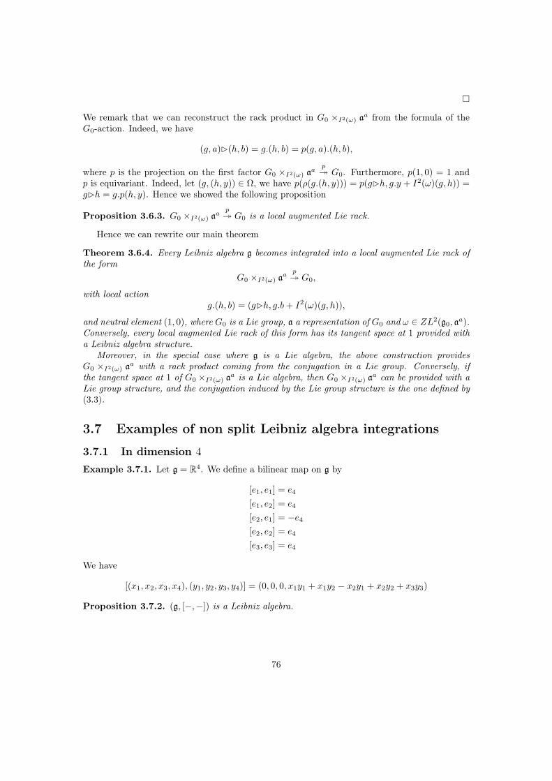
We remark that we can reconstruct the rack product in G0 ×I2(ω) aa from the formula of theG0-action. Indeed, we have

(g, a)⊲(h, b) = g.(h, b) = p(g, a).(h, b),

where p is the projection on the first factor G0 ×I2(ω) aap։ G0. Furthermore, p(1, 0) = 1 and

p is equivariant. Indeed, let (g, (h, y)) ∈ Ω, we have p(ρ(g.(h, y))) = p(g⊲h, g.y + I2(ω)(g, h)) =g⊲h = g.p(h, y). Hence we showed the following proposition

Proposition 3.6.3. G0 ×I2(ω) aap։ G0 is a local augmented Lie rack.

Hence we can rewrite our main theorem

Theorem 3.6.4. Every Leibniz algebra g becomes integrated into a local augmented Lie rack ofthe form

G0 ×I2(ω) aap։ G0,

with local actiong.(h, b) = (g⊲h, g.b+ I2(ω)(g, h)),

and neutral element (1, 0), where G0 is a Lie group, a a representation of G0 and ω ∈ ZL2(g0, aa).

Conversely, every local augmented Lie rack of this form has its tangent space at 1 provided witha Leibniz algebra structure.

Moreover, in the special case where g is a Lie algebra, the above construction providesG0 ×I2(ω) aa with a rack product coming from the conjugation in a Lie group. Conversely, ifthe tangent space at 1 of G0 ×I2(ω) aa is a Lie algebra, then G0 ×I2(ω) aa can be provided with aLie group structure, and the conjugation induced by the Lie group structure is the one defined by(3.3).

3.7 Examples of non split Leibniz algebra integrations

3.7.1 In dimension 4

Example 3.7.1. Let g = R4. We define a bilinear map on g by

[e1, e1] = e4

[e1, e2] = e4

[e2, e1] = −e4

[e2, e2] = e4

[e3, e3] = e4

We have

[(x1, x2, x3, x4), (y1, y2, y3, y4)] = (0, 0, 0, x1y1 + x1y2 − x2y1 + x2y2 + x3y3)

Proposition 3.7.2. (g, [−,−]) is a Leibniz algebra.

76

Proof : We have

[(x1, x2, x3, x4), [(y1, y2, y3, y4), (z1, z2, z3, z4)]] = (0, 0, 0, 0),

and[(y1, y2, y3, y4), [(x1, x2, x3, x4), (z1, z2, z3, z4)]] = (0, 0, 0, 0),

and[[(x1, x2, x3, x4), (y1, y2, y3, y4)], (z1, z2, z3, z4)] = (0, 0, 0, 0).

Hence the bracket [−,−] satisfies the Leibniz identity.

To follow the method explained above, we have to determine the left center ZL(g), the quotientg0 of g by ZL(g) denoted g0, the action of g0 on ZL(g) and the Leibniz 2-cocycle describing theabelian extension ZL(g) → g ։ g0.

Let x ∈ ZL(g), for y = (1, 0, 0, 0), y = (0, 1, 0, 0) or y = (0, 0, 1, 0) in g, we have [x, y] = 0. Thisimplies that x1 = x2 = x3 = 0. Conversely, every element in g with the first three coordinatesequal to 0 is in ZL(g). Hence ZL(g) =< e4 > and g0 ≃< e1, e2, e3 >. The bracket on g0 is equalto zero, hence g0 is an abelian Lie algebra. The action of g0 on ZL(g) is given by

ρx(y) = [(x1, x2, x3, 0), (0, 0, 0, y4)] = (0, 0, 0, 0),

and the Leibniz 2-cocycle is given by

ω(x, y) = [(x1, x2, x3, 0), (y1, y2, y3, 0)] = (0, 0, 0, x1y1 + x1y2 − x2y1 + x2y2 + x3y3).

Now, we have to determine the Lie group G0 associated to g0, the action of G0 on ZL(g) in-tegrating ρ : g0 → End(ZL(g)) (the action of g0 on ZL(g)), and the Lie rack cocycle integrating ω.

The Lie algebra g0 is abelian, thus a Lie group integrating g0 is G0 = g0. Moreover, ρ is nullhence the Lie group action of G0 on ZL(g) which integrates ρ is the trivial action. The facts that ρis zero and g0 abelian, imply that d1

L : CL1(g0, ZL(g)) → CL2(g0, ZL(g)) is zero. Hence, becausegann = ZL(g), g is non split. That is, g is not isomorphic to the direct sum of a Lie algebra h

and a Lie representation V over h provided with the bracket [(x, v), (y, w)] = ([x, y], x.w) (seethe introduction). What remains to be done is the integration of the cocycle ω. A formula forf , a Lie rack cocycle integrating ω, is

f(a, b) =

∫

γb

(

∫

γa

τ2(ω)eq)eq,

where γa(s) = sa and γb(t) = tb. Let a ∈ G0 and x, y ∈ g0. We have∫

γa

τ2(ω)eq =

∫

[0,1]

τ2(ω)eq(γa(s))(∂

∂s

∣∣∣∣s=0

γa(s))ds

=

∫

[0,1]

Φγa(s)(τ2(ω)(a))ds

=

∫

[0,1]

τ2(ω)(a)ds

= τ2(ω)(a).

77

Thus

f(a, b) =

∫

γb

(τ2(ω)(a))eq

=

∫

[0,1]

γ∗b (τ2(ω)(a))eq

=

∫

[0,1]

τ2(ω)(a))eq(γb(t))(∂

∂t

∣∣∣∣t=0

γb(t))dt

=

∫

[0,1]

τ2(ω)(a))(b)dt

= τ2(ω)(a)(b)

= ω(a, b).

Hence, the conjugation in G0 ×f ZL(g) = R4 is given by

(a1, a2, a3, a4)⊲(b1, b2, b3, b4) = (b1, b2, b3, a1b1 + a2b2 + a3b3 + a1b2 − a2b1 + b4).

We have

∂2

∂s∂t |s,t=0(sa1, sa2, sa3, sa4)⊲(tb1, tb2, tb3, tb4) =

∂2

∂s∂t |s,t=0(tb1, tb2, tb3, st(a1b1 + a2b2 + a3b3 + a1b2 − a2b1), tb4)

= (0, 0, 0, a1b1 + a2b2 + a3b3 + a1b2 − a2b1)

= [(a1, a2, a3, a4), (b1, b2, b3, b4)].

Thus (R4,⊲) integrates (R4, [−,−]).

Example 3.7.3. Let g = R4. We define a bilinear map on g by

[e1, e1] = e2

[e1, e2] = e3

[e1, e3] = e4

We have[(x1, x2, x3, x4), (y1, y2, y3, y4)] = (0, x1y1, x1y2, x1y3)

Proposition 3.7.4. (g, [−,−]) is a Leibniz algebra.

Proof : We have

[(x1, x2, x3, x4), [(y1, y2, y3, y4), (z1, z2, z3, z4)]] = [(x1, x2, x3, x4), (0, y1z1, y1z2, y1z3)]

= (0, 0, x1y1z2, x1y1z3),

and[(y1, y2, y3, y4), [(x1, x2, x3, x4), (z1, z2, z3, z4)]] = (0, 0, x1y1z2, x1y1z3),

and[[(x1, x2, x3, x4), (y1, y2, y3, y4)], (z1, z2, z3, z4)] = 0.

Hence the bracket [−,−] satisfies the Leibniz identity.

78

To follow the method explained above, we have to determine the left center ZL(g), the quotientg0 of g by ZL(g) denoted g0, the action of g0 on ZL(g) and the Leibniz 2-cocycle describing theabelian extension ZL(g) → g ։ g0.

Let x ∈ ZL(g), for y = (1, 0, 0, 0), y = (0, 1, 0, 0) or y = (0, 0, 1, 0) in g, we have [x, y] = 0.This implies that x1 = 0. Conversely, every element in g with the first coordinate equals to 0is in ZL(g). Hence ZL(g) =< e2, e3, e4 > and g0 ≃< e1 >. The bracket on g0 is equal to zero,hence g0 is an abelian Lie algebra. The action of g0 on ZL(g) is given by

ρx(y) = [(x1, 0, 0, 0), (0, y2, y3, y4)] = (0, 0, x1y2, x1y3),

and the Leibniz 2-cocycle is given by

ω(x, y) = [(x1, 0, 0, 0), (y1, 0, 0, 0)] = (0, x1y1, 0, 0).

Moreover, we have [x, x] = (0, x21, x1x2, x1x3), hence gann = ZL(g). This Leibniz algebra

is not split because for α ∈ Hom(g0,R) and x, y ∈ g0, we have dLα(x, y) = ρx(α(y)) =(0, 0, x1α(y)2, x1α(y)3).

Now, we have to determine the Lie group G0 associated to g0, the action of G0 on ZL(g) in-tegrating ρ : g0 → End(ZL(g)) (the action of g0 on ZL(g)), and the Lie rack cocycle integrating ω.

The Lie algebra g0 is abelian, thus a Lie group integrating g0 is G0 = g0. Moreover, a simplecalculation shows that the Lie group action of G0 on ZL(gg) defined by

φx(y) = y + ρx(y),

integrates ρ. What remains to be done is the integration of the cocycle ω. A formula for f , aLie rack cocycle integrating ω, is

f(a, b) =

∫

γb

(

∫

γa

τ2(ω)eq)eq,

79

where γa(s) = sa and γb(t) = tb. Let a ∈ G0 and x, y ∈ g0. We have∫

γa

τ2(ω)eq =

∫

[0,1]

τ2(ω)eq(γa(s))(∂

∂s

∣∣∣∣s=0

γa(s))ds

=

∫

[0,1]

Φγa(s)(τ2(ω)(a))ds

=

∫

[0,1]

φγa(s) τ2(ω)(a)ds

=

∫

[0,1]

0asa2

0

ds

=

0a00

+

1

2

00a2

0

=

0a

12a

2

0

.

Thus

f(a, b) =

∫

γb

(

0a

12a

2

0

)eq

=

∫

[0,1]

γ∗b (

0a

12a

2

0

)eq.

f(a, b) =

∫

[0,1]

0a

12a

2

0

eq

(γb(t))(∂

∂t

∣∣∣∣t=0

γb(t))dt

=

∫

[0,1]

φγb(t)(

0a

12a

2

0

(b))dt

=

∫

[0,1]

abe2 + (tab2 +1

2a2b)e3 +

1

2ta2b2e4dt

= abe2 +1

2(ab2 + a2b)e3 +

1

4a2b2e4.

Hence, the conjugation in G0 ×f ZL(g) = R4 is given by

(a1, a2, a3, a4)⊲(b1, b2, b3, b4) = (b1, a1b1, a1b2 +1

2(a1b

21 + a2

1b1), a1b3 +1

4a21b

21).

80

We have

∂2

∂s∂t |s,t=0(sa1, sa2, sa3, sa4)⊲(tb1, tb2, tb3, tb4) =

∂2

∂s∂t |s,t=0(tb1, sta1b1, sta1b2 +

1

2(st2a1b

21 + s2ta2

1b1),

sta1b3 + s2t21

4a21b

21)

= (0, a1b1, a1b2, a1b3)

= [(a1, a2, a3, a4), (b1, b2, b3, b4)].

Thus (R4,⊲) integrates (R4, [−,−]).

3.7.2 In dimension 5

Example 3.7.5. Let g = R5. We define a bilinear map on g by

[e1, e1] = [e1, e2] = e3

[e2, e1] = [e2, e2] = [e1, e3] = e4

[e1, e4] = [e2, e3] = e5

We have

[(x1, x2, x3, x4), (y1, y2, y3, y4)] = (0, 0, x1(y1 + y2), x2(y1 + y2) + x1y3, x1y4 + x2y3).

Proposition 3.7.6. (g, [−,−]) is a Leibniz algebra.

Proof : We have

[(x1, x2, x3, x4), [(y1, y2, y3, y4), (z1, z2, z3, z4)]] = (0, 0, 0, x1y1(z1+z2), x1(y2(z1+z2)+y1z3)+x2y1(z1+z2)),

and

[(y1, y2, y3, y4), [(x1, x2, x3, x4), (z1, z2, z3, z4)]] = (0, 0, 0, x1y1(z1+z2), x1(y2(z1+z2)+y1z3)+x2y1(z1+z2)),

and[[(x1, x2, x3, x4), (y1, y2, y3, y4)], (z1, z2, z3, z4)] = (0, 0, 0, 0).

Hence the bracket [−,−] satisfies the Leibniz identity.

To follow the method explained above, we have to determine the left center ZL(g), the quotientof g by ZL(g) denoted g0, the action of g0 on ZL(g) and the Leibniz 2-cocycle describing theabelian extension ZL(g) → g ։ g0.

Let x ∈ ZL(g), for y = (0, 0, 1, 0, 0) in g, we have [x, y] = 0. This implies that x1 = x2 = 0.Conversely, every element in g with the first two coordinates equal to 0 is in ZL(g). HenceZL(g) =< e3, e4, e5 > and g0 ≃< e1, e2 >. The bracket on g0 is equal to zero, hence g0 is anabelian Lie algebra. The action of g0 on ZL(g) is given by

ρx(y) = [(x1, x2, 0, 0, 0), (0, 0, y3, y4, y5)] = (0, 0, 0, x1y3, x1y4 + x2y3),

and the Leibniz 2-cocycle is given by

ω(x, y) = [(x1, x2, 0, 0, 0), (y1, y2, 0, 0, 0)] = (0, 0, x1(y1 + y2), x2(y1 + y2), 0).

81

Moreover, we have [x, x] = (0, 0, x1(x1 + x2), x2(x1 + x2) + x1x3, x1x4 + x2x3), hence takingx = (1, 0, 0, 0, 0), (0, 1, 0, 0, 0) and (0, 1, 1, 0, 0), we see easily that gann = ZL(g). This Leibniz al-gebra is not split because for α ∈ Hom(g, ZL(g)) and x, y ∈ g0, we have dLα(x, y) = ρx(α(y)) =(0, 0, 0x1α(y)3, x1α(y)4 + x2α(y)3).

Now, we have to determine the Lie group G0 associated to g0, the action of G0 on ZL(g) in-tegrating ρ : g0 → End(ZL(g)) (the action of g0 on ZL(g)), and the Lie rack cocycle integrating ω.

The Lie algebra g0 is abelian, thus a Lie group integrating g0 is G0 = g0. To integrate theaction ρ, we use the exponential exp : End(ZL(g)) → Aut(ZL(g)). Indeed, for all x ∈ g0, wehave

ρx =

0 0 0x1 0 0x2 x1 0

.

Hence, we define a Lie group morphism φ : G0 → Aut(ZL(g)) by setting

φx = exp(ρx) =

1 0 0x1 1 0

x2 + 12x

21 x1 0

.

It is easy to see that d1φ = ρ. What remains to be done is the integration of the cocycle ω. Aformula for f , a Lie rack cocycle integrating ω, is

f(a, b) =

∫

γb

(

∫

γa

τ2(ω)eq)eq,

where γa(s) = sa and γb(t) = tb. Let a ∈ G0 and x, y ∈ g0. We have

∫

γa

τ2(ω)eq =

∫

[0,1]

τ2(ω)eq(γa(s))(∂

∂s

∣∣∣∣s=0

γa(s))ds

=

∫

[0,1]

Φγa(s)(τ2(ω)(a))ds

=

∫

[0,1]

φγa(s) τ2(ω)(a)ds

=

∫

[0,1]

1 0 0sa1 1 0

sa2 + 12 (sa1)

2 sa1 0

a1 a1

a2 a2

0 0

ds

=

∫

[0,1]

a1 a1

sa21 + a2 sa2

1 + a2

2sa1a2 + 12s

2a31 2sa1a2 + 1

2s2a3

1

ds.

Thus∫

γa

τ2(ω)eq =

a1 a112a

21 + a2

12a

21 + a2

a1a2 + 16a

31 a1a2 + 1

6a31

.

82

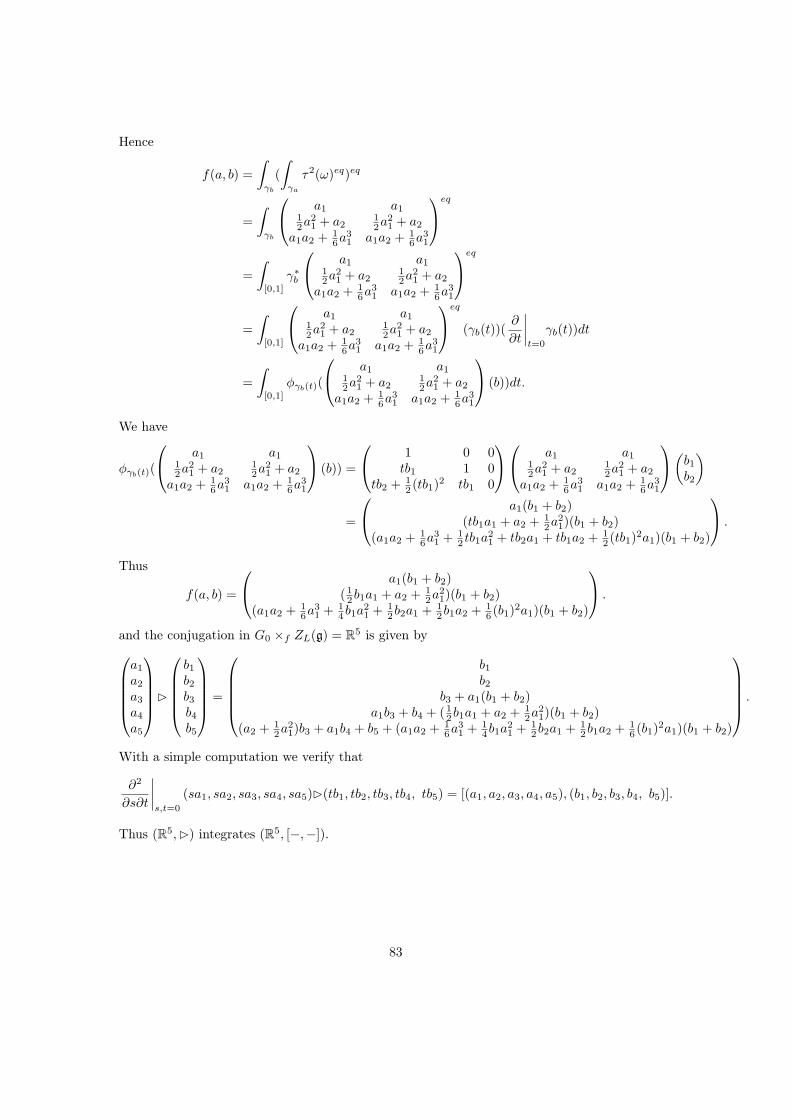
Hence

f(a, b) =

∫

γb

(

∫

γa

τ2(ω)eq)eq

=

∫

γb

a1 a112a

21 + a2

12a

21 + a2

a1a2 + 16a

31 a1a2 + 1

6a31

eq

=

∫

[0,1]

γ∗b

a1 a112a

21 + a2

12a

21 + a2

a1a2 + 16a

31 a1a2 + 1

6a31

eq

=

∫

[0,1]

a1 a112a

21 + a2

12a

21 + a2

a1a2 + 16a

31 a1a2 + 1

6a31

eq

(γb(t))(∂

∂t

∣∣∣∣t=0

γb(t))dt

=

∫

[0,1]

φγb(t)(

a1 a112a

21 + a2

12a

21 + a2

a1a2 + 16a

31 a1a2 + 1

6a31

(b))dt.

We have

φγb(t)(

a1 a112a

21 + a2

12a

21 + a2

a1a2 + 16a

31 a1a2 + 1

6a31

(b)) =

1 0 0tb1 1 0

tb2 + 12 (tb1)

2 tb1 0

a1 a112a

21 + a2

12a

21 + a2

a1a2 + 16a

31 a1a2 + 1

6a31

(b1b2

)

=

a1(b1 + b2)(tb1a1 + a2 + 1

2a21)(b1 + b2)

(a1a2 + 16a

31 + 1

2 tb1a21 + tb2a1 + tb1a2 + 1

2 (tb1)2a1)(b1 + b2)

.

Thus

f(a, b) =

a1(b1 + b2)( 12b1a1 + a2 + 1

2a21)(b1 + b2)

(a1a2 + 16a

31 + 1

4b1a21 + 1

2b2a1 + 12b1a2 + 1

6 (b1)2a1)(b1 + b2)

.

and the conjugation in G0 ×f ZL(g) = R5 is given by

a1

a2

a3

a4

a5

⊲

b1b2b3b4b5

=

b1b2

b3 + a1(b1 + b2)a1b3 + b4 + ( 1

2b1a1 + a2 + 12a

21)(b1 + b2)

(a2 + 12a

21)b3 + a1b4 + b5 + (a1a2 + 1

6a31 + 1

4b1a21 + 1

2b2a1 + 12b1a2 + 1

6 (b1)2a1)(b1 + b2)

.

With a simple computation we verify that

∂2

∂s∂t

∣∣∣∣s,t=0

(sa1, sa2, sa3, sa4, sa5)⊲(tb1, tb2, tb3, tb4, tb5) = [(a1, a2, a3, a4, a5), (b1, b2, b3, b4, b5)].

Thus (R5,⊲) integrates (R5, [−,−]).

83

84

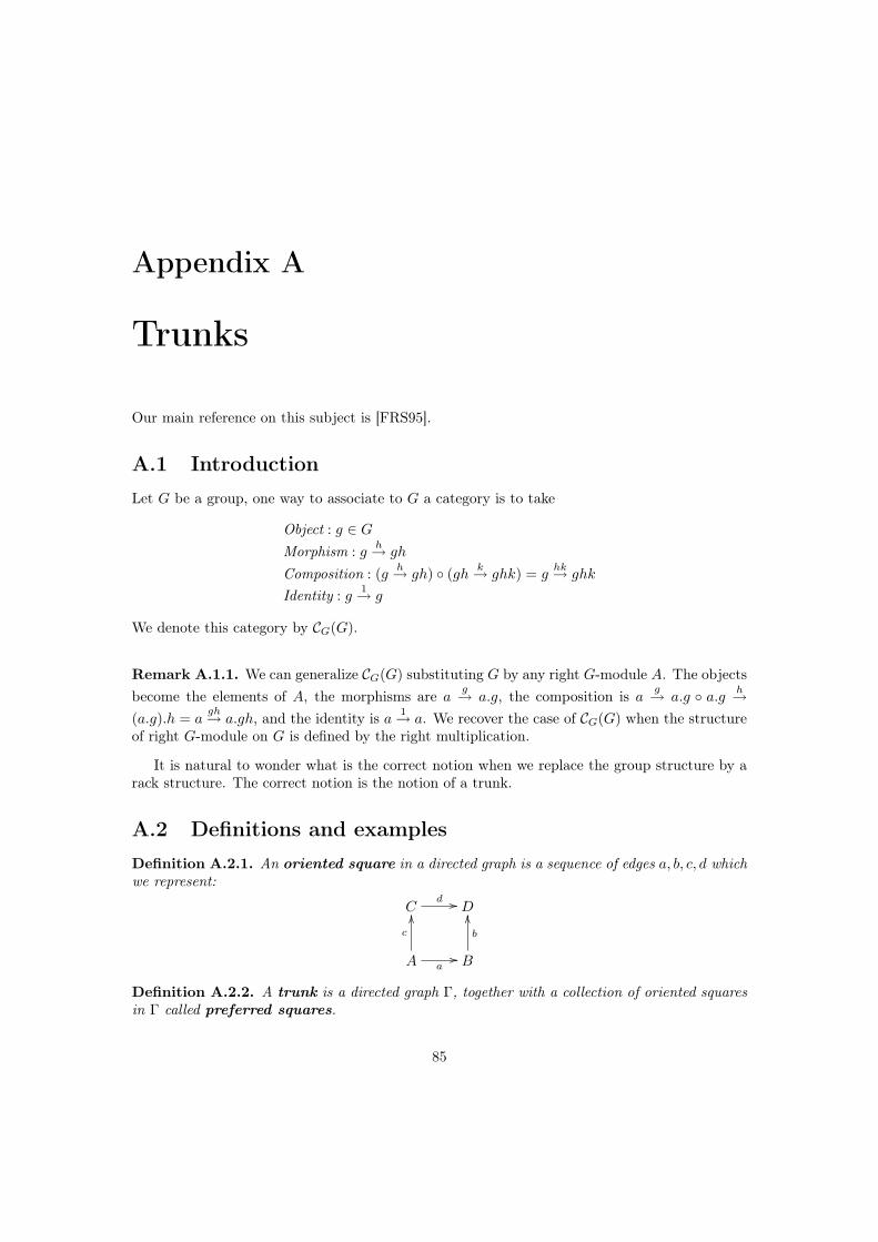
Appendix A

Trunks

Our main reference on this subject is [FRS95].

A.1 Introduction

Let G be a group, one way to associate to G a category is to take

Object : g ∈ G

Morphism : gh→ gh

Composition : (gh→ gh) (gh

k→ ghk) = g

hk→ ghk

Identity : g1→ g

We denote this category by CG(G).

Remark A.1.1. We can generalize CG(G) substituting G by any right G-module A. The objects

become the elements of A, the morphisms are ag→ a.g, the composition is a

g→ a.g a.g

h→

(a.g).h = agh→ a.gh, and the identity is a

1→ a. We recover the case of CG(G) when the structure

of right G-module on G is defined by the right multiplication.

It is natural to wonder what is the correct notion when we replace the group structure by arack structure. The correct notion is the notion of a trunk.

A.2 Definitions and examples

Definition A.2.1. An oriented square in a directed graph is a sequence of edges a, b, c, d whichwe represent:

Cd // D

A a//

c

OO

B

b

OO

Definition A.2.2. A trunk is a directed graph Γ, together with a collection of oriented squaresin Γ called preferred squares.

85

Definition A.2.3. A pointed trunk is a trunk together with a chosen edge eA : A → A foreach vertex A, and with the following preferred squares for each edge a : A→ B.

Aa // B B

eB // B

A a//

eA

OO

B

eB

OO

A

a

OO

eA

// A

a

OO

The edges eA are called the identities.

Definition A.2.4. A corner trunk is a trunk which satisfies the following two corner axioms:

(C1) Given edges a : A → B and b : B → D, there are unique edges a⊲b : A → C anda⊳ b : C → D such that the following square is preferred

Ca⊳b // D

A

a⊲b

OO

a// B

b

OO

(C2) In the following diagram, if the squares (ABCD), (BDY T ) and (CDZT ) are preferred,then the diagram can be completed as shown so that the squares (ABXY ), (ACXZ) and(XY ZT ) are preferred.

Z // T

X //

>>

Y

>>~

~~

~~

~~

C //

OO

D

c

OO

A a//

>>~

~~

~~

~~

OO

B

b

>>~

~~

~~

~~

OO

Given (C1), an equivalent statement is that the edges a, b and c determine the entire dia-gram of preferred squares.

Proposition A.2.5. In a corner trunk, the binary operations ⊲ and ⊳ satisfy:

1. a⊲(b⊲c) = (a⊲b)⊲((a⊳ b)⊲c)

2. (a⊳ b) ⊳ c) = (a⊳ (b⊲c)) ⊳ (b⊳ c)

3. (a⊳ (b⊲c))⊲(b⊳ c) = (a⊲b) ⊳ ((a⊳ b)⊲c)

Definition A.2.6. Let S and T two trunks. A trunk map between T and S maps verticeson vertices, edges on edges and preferred squares on preferred squares. If S and T are pointedtrunks, then a pointed trunk map between T and S is a trunk map from T to S which takesidentities to identities.

86

Example A.2.7 (Category). Let C be a category. We define a directed graph Γ(C) using C bytaking the objects as vertices, and the morphisms as edges. Hence, we define a trunk Trunk(C)by taking the commutative squares in C as preferred squares. Moreover, this trunk is a pointedtrunk using the identity morphisms in C.

This construction gives a functor between the category of categories and the category of(pointed) trunks. Conversely, we can define a functor from the category of (pointed) trunks tothe category of categories. We take as objects the vertices, and the morphisms are generatedby the edges of the trunk with the relations which follows from insisting that preferred squarescommute (and identifying the identities in the trunk with identites in the category for the pointedversion). Then, this functor, denoted Cat, is left adjoint to the functor Trunk.

Example A.2.8 (The rack trunk). This is the key example. Let X be a rack, we define a cornertrunk T (X) by setting

Vertices: ∗

Edges: for all x ∈ X, ∗x→ ∗

Preferred squares: for all x, y ∈ X,

∗x // ∗

∗

x⊲y

OO

x// ∗

y

OO

The corner trunk axioms are satisfied because of the axioms defining a rack. Indeed, by defini-tion of this trunk, the axiom (C1) is clear, and, because of the rack identity, the axiom (C2) issatisfied. Moreover, if we suppose that X is a pointed rack, then T (X) is a pointed corner trunkwith identity 1.

Example A.2.9 (The augmented rack trunk). Let Xp→ G be an augmented rack, we define a

corner trunk TG(X) by setting

Vertices: g ∈ G

Edges: for all g ∈ G, x ∈ X, gx→ gp(x)

Preferred squares: for all g ∈ G, x, y ∈ X,

gp(x⊲y)x // gp(x)p(y)

g

x⊲y

OO

x// gp(x)

y

OO

Moreover, if we suppose that this augmented rack is pointed, then TG(X) is a pointed cornertrunk with identity 1.

Example A.2.10 (the n-cube). We define for all n ∈ N a corner trunk, called n-cube anddenoted n, by setting

87

Vertices: subsets of 1, . . . , n

Edges: Vi→ V ∪ i where i /∈ V

Preferred squares: for all i < j

V ∪ ji // V ∪ i ∪ j

V

j

OO

i // V ∪ i

j

OO

Another description of this trunk is

Vertices: n-uplets (ǫ1, . . . , ǫn) where ǫi ∈ 0, 1

Edges: for all i ∈ 1, . . . , n, (ǫ1, . . . , ǫi−1, ǫi, ǫi+1, . . . , ǫn)i→ (ǫ1, . . . , ǫi−1, ǫ

′i, ǫi+1, . . . , ǫn) where

ǫ′i = 1.

Preferred squares: for all i < j

(ǫ1, . . . , ǫ′′j , . . . , ǫn) i // (ǫ1, . . . , ǫ′i, . . . , ǫ

′′j , . . . , ǫn)

(ǫ1, . . . , ǫn)

j

OO

i // (ǫ1, . . . , ǫ′i, . . . , ǫn)

j

OO

Moreover, we define for all n ∈ N a pointed corner trunk +n by deleting the hypothesis i /∈ V in

the first definition of the vertices. Hence, the identities are Vid→ V .

A.3 The category +

Objects: We take as objects the trunks +n defined above.

Morphisms: To define the morphisms in this category, we have to define two kinds of maps,the face maps and the degeneracies.

Face maps: a (n− 1)-face is a map ǫi,α : +n → +

n given by

ǫi,α(ǫ1, . . . , ǫn−1) = (ǫ1, . . . , ǫi−1, α, ǫi, . . . , ǫn−1)

A composition of such (n− 1)-faces is called a face map.Example: For i = 1, α = 1, we can represent ǫ1,1 by

∗ ∗

∗ ∗ ∗ ∗

ǫ1,1 // ∗ ∗

∗ ∗ ∗ ∗

88

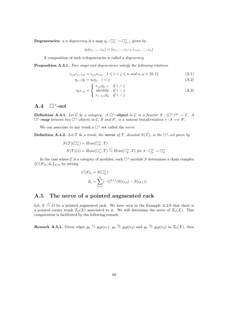
Degeneracies: a n-degeneracy is a map ηi : +n →

+n−1 given by

ηi(ǫ1, . . . , ǫn) = (ǫ1, . . . , ǫi−1, ǫi+1, . . . , ǫn)

A composition of such n-degeneracies is called a degeneracy.

Proposition A.3.1. Face maps and degeneracies satisfy the following relations

ǫi,αǫj−1,ω = ǫj,ωǫi,α, 1 6 i < j 6 n and α, ω ∈ 0, 1 (A.1)

ηj−1ηi = ηiηj , i < j (A.2)

ηjǫi,α =

ǫi,αηj−1 if i < jidentity if i = jǫi−1,αηj if i > j

(A.3)

A.4 +-set

Definition A.4.1. Let C be a category. A +-object in C is a functor S : (+)op → C. A+-map between two +-objects in C, S and S′, is a natural transformation τ : S =⇒ S′.

We can associate to any trunk a +-set called the nerve.

Definition A.4.2. Let T be a trunk, the nerve of T , denoted N(T ), is the +-set given by

N(T )(+n ) = Hom(+

n , T )

N(T )(λ) = Hom(+n , T )

λ∗

→ Hom(+p , T ) for λ :

+p →

+n

In the case where C is a category of modules, each +-module S determines a chain complexC(S)n, dnn≥0 by setting

C(S)n = S(+n )

∂n =n∑

k=1

(−1)k+1(S(ǫk,0) − S(ǫk,1))

A.5 The nerve of a pointed augmented rack

Let Xp→ G be a pointed augmented rack. We have seen in the Example A.2.9 that there is

a pointed corner trunk TG(X) associated to it. We will determine the nerve of TG(X). Thiscomputation is facilitated by the following remark.

Remark A.5.1. Given edges g0x1→ g0p(x1), g0

x2→ g0p(x2) and g0x3→ g0p(x3) in TG(X), then

89

there exists a unique way to complete the diagram

∗ // ∗

g0p(x3) //

99

∗

;;

g0p(x2) //

OO

∗

OO

g0x1 //

x3

OO

x2

99t

tt

tt

tt

tt

tt

g0p(x1)

OO

<<

into a diagram of preferred squares. An equivalent statement is to say that we have the identity

c−1x1

c−1x2

= c−1

c−1x1

(x2) c−1

x1

Proposition A.5.2. Let Xp→ G be a pointed corner trunk. We have a bijection

N(TG(X))(+n )

tn→ G×Xn,∀n ∈ N

and

N(TG(X))(ǫi,0)(g0, x1, . . . , xn) = (g0, x1, . . . , xi⊲xi+1, . . . , xi⊲xn)

N(TG(X))(ǫi,1)(g0, x1 . . . , xn) =(g0p(x1⊲ . . .⊲xi), x1, . . . , xi, . . . , xn

)

N(TG(X))(ηi)(g0, x1, . . . , xn) = (g0, x1, . . . , xi−1, 1, xi, . . . , xn)

Proof : Let F ∈ N(TG(X))(+n ), we define an element (g0, x1, . . . , xn) ∈ G × Xn by setting

g0 = F (∅) and

xk = F (1, . . . , k − 1)i→ F (1, . . . , k)

Conversely, let (g0, x1, . . . , xn), we define an element F on the subsets 1, . . . , k of 1, . . . , nby setting

F (1, . . . , k = g0p(x1) . . . p(xk)

these data allow us to define F on the subsets k. Indeed, we have the following diagram ofpreferred square in +

n

k1 // 1, k

2 // 1, 2, k // // 1, . . . , k − 2, kk−1 // 1, . . . , k

∅1 //

k

OO

12 //

k

OO

1, 2

k

OO

// // 1, . . . , k − 2k−1 //

k

OO

1, . . . , k − 1

k

OO

Hence, by the corner axiom (C1), if we want F to be a trunk map, we have a unique choice forF (k). Thus, F is determined on k for all 1 ≤ k ≤ n.Now we can construct F by induction on the cardinality of the subsets of 1, . . . , n. Suppose

90

that F is known on the subset of 1, . . . , n of cardinal lower than l. Let A be a subset of1, . . . , n of cardinal l, i /∈ A and B ⊂ A of cardinal l − 1. The square

Ai // A ∪ i

B

OO

i // B ∪ i

OO

is preferred in +n . We want that F sends preferred squares to preferred squares, hence by using

the remark above, we have a unique choice to define the edge F (A) → F (A ∪ i). To showthat this is well defined, we have to show that our construction does not depend on the chosensubset B. Suppose that A = B1 ∪ j = B2 ∪ k and let B = B1 ∩ B2 so that A = B ∪ j, kand suppose, without loss of generality, that j < k. We have the following diagram of preferredsquares in +

n

B ∪ i, k // A ∪ i

B ∪ k //

88r

rr

rr

rr

rr

r

A

88r

rr

rr

rr

rr

rr

r

B ∪ i //

OO

B ∪ i, j

OO

B //

OO

88

B ∪ j

OO

88r

rr

rr

rr

rr

r

By induction, F is defined on the three edges originating at B. Hence if we want F to be a trunkmap, by using the remark above F (A) → F (A ∪ i) is well defined.

Let (g0, x1, . . . , xn) ∈ G × Xn and let F be the element of N(TG(X)) associated to this(n + 1)-tuple. We have for all 1 ≤ k ≤ n, ǫi,0(1, . . . , k) = 1, . . . , i − 1, i + 1, . . . , k + 1. Wehave the following diagram of preferred squares in +

n

1, . . . , i− 1 //

1, . . . , i− 1, i+ 1

1, . . . , i− 1, i+ 1, . . . , k //

1, . . . , i− 1, i+ 1, . . . k + 1

1, . . . , i // 1, . . . , i+ 1 1, . . . , k // 1, . . . , k + 1

F is a trunk map, thus it sends this diagram to the following diagram of preferred squares inTG(X)

g0p(x1) . . . p(xi−1) //

xi

F (ǫi,0(1, . . . , i))

xi

F (ǫi,0(1, . . . , k − 1)) //

xi

F (ǫi,0(1, . . . , k))

xi

g0p(x1) . . . p(xi)

xi+1 // g0p(x1) . . . p(xi+1) g0p(x1) . . . p(xk)xk // g0p(x1) . . . p(xk+1)

Thus F (ǫi,0(1, . . . , k − 1)) → F (ǫi,0(1, . . . , k)) is equal to xi⊲xk if i ≤ k and xi if i > k.Hence

N(TG(X))(ǫi,0)(g0, x1, . . . , xn) = (g0, x1, . . . , xi⊲xi+1, . . . , xi⊲xn)

91

Moreover, we have for all 1 ≤ k ≤ n, ǫi,1(1, . . . , k) = 1, . . . , k+1 if i ≤ k and ǫi,1(1, . . . , k) =1, . . . , k, i if i > k. Thus F (ǫi,1(1, . . . , k− 1)) → F (ǫi,1(1, . . . , k)) is equal to xk+1 if i ≤ k.For i > k, we have the following preferred square

1, . . . , k − 1, i // 1, . . . , k, i

1, . . . , k − 1

OO

// 1, . . . , k

OO

Thus F (ǫi,1(1, . . . , k − 1)) → F (ǫi,1(1, . . . , k) = F (1, . . . , k − 1) → F (1, . . . , k) = xk. Itremains to determine F (ǫi,1(∅)). We have ǫi,1(∅) = i and the following diagram is a diagramof preferred squares in TG(X).

F (i)x1 // F (1, i)

x2 // // F (1, . . . , i− 2, i)xi−1 // F (1, . . . , i)

F (∅)x1 //

x1⊲...⊲xi

OO

F (1)x2 //

x2⊲...⊲xi

OO

// F (1, . . . , i− 2)xi−1 //

xi−1⊲xi

OO

F (1, . . . , i− 1)

xi

OO

Thus by the corner axiom (C1), F (ǫi,1(∅)) = g0p(x1⊲ . . .⊲xi) and

N(TG(X))(ǫi,1)(g0, x1 . . . , xn) =(g0p(x1⊲ . . .⊲xi), x1, . . . , xi, . . . , xn

)

Furthermore, we have for all 1 ≤ k ≤ n, ηi(1, . . . , k) = 1, . . . , k−1 if i ≤ k and ηi(1, . . . , k) =1, . . . , k if i > k. Thus F (ηi(1, . . . , k − 1)) → F (ηi(1, . . . , k)) is equal to xk−1 if i > kand is equal to xk if i < k. For i = k, we have F (ηk(1, . . . , k − 1)) → F (ηk(1, . . . , k)) =F (1, . . . , k − 1) → F (1, . . . , k − 1) = 1. Hence

N(TG(X))(ηi)(g0, x1, . . . , xn) = (g0, x1, . . . , xi−1, 1, xi, . . . , xn).

We denote N(TG(X))(+n ) by Γn

G(X), N(TG(X))(ǫi,α) by ∂i,α and N(TG(X))(ηi) by σi.

Proposition A.5.3. For all n ∈ N, we define an action of G on ΓG(X) by setting

g.(g0, x1, . . . , xn) = (gg0, x1, . . . , xn).

Moreover, the action preserves the maps ∂i,α and σi, that is for all γ ∈ ΓG(X)

g.∂i,α(γ) = ∂i,α(g.γ),

andg.σi(γ) = σi(g.γ).

Let A be a G-module. We denote by En(ΓG(X), A) the set of functions from ΓnG(X) to A

which are equivariant for the action of G, and such that f σi = 0, for all 1 ≤ i ≤ n. We definea cochain complex En(ΓG(X), A), dn

Γn∈N by setting

dnΓf =

n∑

i=1

(−1)i+1(di,1Γ f − di,0

Γ f),

where di,αΓ f = f ∂i,α.

Lemma A.5.4. dn+1Γ dn

Γ = 0.

Proof : This is clear using the identities (A.1).

92

A.6 Relation with pointed rack cohomology

Let X be a pointed rack. We have seen in Example 2.1.24 that there is a canonical pointedaugmented rack associated to X, it is X

µ→ Asp(X). Recall that on an Asp(X)-module

A, we can define the structure of symmetric X-pointed module. The following propositionestablishes an isomorphism between the cochain complexes En(ΓAsp(X)(X), A), dn

Γn∈N andCRn

p (X,As), dnRn∈N.

Proposition A.6.1. Let X be a pointed rack and let A be an Asp(X)-module. We have anisomorphism of cochain complexes

En(ΓAsp(X)(X), A)νn

→ CRnp (X,As),

given byνn(f)(x1, . . . , xn) = f([1], x1, . . . , xn),

with inverse given by

(νn)−1(f)([w], x1, . . . , xn) = [w].f(x1, . . . , xn).

Proof : Let f ∈ En(ΓAsp(X)(X), A) and (x1, . . . , xn) ∈ Xn. We have

dnRν

n(f)(x1, . . . , xn+1) =

n∑

i=1

(−1)n+1(φx1⊲...,⊲xi

(νn(f)(x1, . . . , xi, . . . , xn+1)

− νn(f)(x1, . . . , xi−1, xi⊲xi+1, . . . , xi⊲xn+1))

=n∑

i=1

(−1)n+1(φx1⊲...,⊲xi

(f([1], x1, . . . , xi, . . . , xn+1)

− f([1], x1, . . . , xi−1, xi⊲xi+1, . . . , xi⊲xn+1))

=n∑

i=1

(−1)n+1((f([x1⊲ . . . ,⊲xi], x1, . . . , xi, . . . , xn+1)

− f([1], x1, . . . , xi−1, xi⊲xi+1, . . . , xi⊲xn+1)),

and

νn+1(dnΓf)(x1, . . . , xn+1) = dn

Γf([1], x1, . . . , xn+1)

=

n∑

i=1

(−1)i+1(di,1Γ f − di,0

Γ f)([1], x1, . . . , xn+1)

=

n∑

i=1

(−1)i+1(f ǫi,1 − f ǫ0,α)([1], x1, . . . , xn+1)

=

n∑

i=1

(−1)i+1(f([x1⊲ . . . ,⊲xi], x1, . . . , xi, . . . , xn+1)

− f([1], x1, . . . , xi−1, xi⊲xi+1, . . . , xi⊲xn+1)).

Thus νnn∈N is an isomorphism of cochain complexes.

93

A.7 Relation with group cohomology

Let G be a group, Proposition 2.3.24 establishes that there is a morphism from the group coho-mology of G to the pointed rack cohomology of Conj(G). Here we give a proof of this theoremusing trunk theory.

The +-complex associated to a group

We can see a group as the pointed augmented rack Conj(G)id→ G, thus if we have a G-module

A, we can talk about En(ΓG(Conj(G)), A), dnΓn∈N.

Proposition A.7.1. We have an isomorphism of cochain complexes

En(ΓG(G), A)tn

→ En(ΓAs(Conj(G)(Conj(G)), A),

given bytn(f)([w], g1, . . . , gn) = [w].f(1, g1, . . . , gn),

with inverse given by

(tn)−1(f)(g0, g1, . . . , gn) = f([g0], g1, . . . , gn).

Hence, by combining Proposition A.6.1 and Proposition A.7.1, we have the following result

Proposition A.7.2. We have an isomorphism of cochain complexes

En(ΓG(G), A)θn

→ CRnp (G,As),

given byθn(f)(g1, . . . , gn) = f(1, g1, . . . , gn),

with inverse given by(θn)−1(f)(g0, . . . , gn) = g0.f(g1, . . . , gn).

The ∆-complex associated to a group

In the introduction we have associated a category to a group G. We can use this constructionto associate to G a simplicial complex with an action of the group G. By taking the equivariantmap from this simplical complex to a G-module A, we construct a cochain complex and we canshow that there exists an isomorphism between this complex and the complex defining the groupcohomology of G.

Let G be a group. Recall the description of the category CG(G)

Objects: g ∈ G

Morphisms: gh→ gh

Composition: gh→ gh gh

k→ ghk = g

ghk→ ghk

Identity: g1→ g

94

The nerve of the category CG(G) is the simplicial set N(CG(G)) defined by

N(CG(G))(∆n) = Hom(∆n, CG(G))

N(CG(G))(λ) = Hom(∆n, CG(G))λ∗

→ Hom(∆p, CG(G)) for λ : ∆p → ∆n

Proposition A.7.3. Let G be a group. We have a bijection

N(CG(G))(∆n)tn∆→ Gn+1,∀n ∈ N,

and under this isomorphism

N(CG(G))(ǫi)(g0, . . . , gn) =

(g1, . . . , gn) if i = 0(g0, . . . , gigi+1, . . . , gn) if 1 ≤ i ≤ n− 1(g0, . . . , gn−1) if i = n

N(CG(G))(ηi)(g0, . . . , gn) = (g0, . . . , 1, . . . , gn)

Proof : For all F ∈ N(CG(G)), we define tn∆(F ) = (g0, g1, . . . , gn) by setting g0 = F (0) and

gi = F (i− 1) → F (i).

Conversely, given a (n+1)-tuple in Gn+1, we define an element ((tn∆)−1)(g0, . . . , gn) in N(CG(G))by setting

((tn∆)−1)(g0, . . . , gn))(i) = g0. . . . .gi.

Hence N(CG(G)) and Gn+1 are in bijection.Moreover, let (g0, . . . , gn) ∈ Gn+1, we have

(N(CG(G)

)(ǫ0)

((tn∆)−1)(g0, . . . , gn)

)(i) = ((tn∆)−1)(g0, . . . , gn))(ǫ0(i))

= ((tn∆)−1)(g0, . . . , gn))(i+ 1).

Thus(tn−1∆ N(CG(G))(ǫ0) (tn∆)−1

)(g0, . . . , gn) = (g1, . . . , gn).

We have(N(CG(G)

)(ǫn)

((tn∆)−1)(g0, . . . , gn)

)(i) = ((tn∆)−1)(g0, . . . , gn))(ǫn(i))

= ((tn∆)−1)(g0, . . . , gn))(i).

Thus(tn−1∆ N(CG(G))(ǫn) (tn∆)−1

)(g0, . . . , gn) = (g0, . . . , gn−1).

Furthermore, for 1 ≤ k ≤ n− 1, we have

(N(CG(G)

)(ǫk)

((tn∆)−1)(g0, . . . , gn)

)(i) =

((tn∆)−1)(g0, . . . , gn)

)(i) if i < k

((tn∆)−1)(g0, . . . , gn))(i+ 1) if i ≥ k

Thus(tn−1∆ N(CG(G))(ǫk) (tn∆)−1

)(g0, . . . , gn) = (g0, . . . , gkgk+1, . . . , gn−1).

To finish, let 1 ≤ k ≤ n, we have

(N(CG(G)

)(ηk)

((tn∆)−1)(g0, . . . , gn)

)(i) =

((tn∆)−1)(g0, . . . , gn)

)(i) if i ≤ k

((tn∆)−1)(g0, . . . , gn))(i− 1) if i > k

Thus(tn−1∆ N(CG(G))(ηk) (tn∆)−1

)(g0, . . . , gn) = (g0, . . . , 1, . . . , gn−1).

95

We denote N(CG(G))(∆n) by ΣnG(G), N(CG(G))(ǫi) by ∂i and N(CG(G))(ηi) by σi.

Proposition A.7.4. For all n ∈ N, we define an action of G on ΣG(G) by setting

g.(g0, g1, . . . , gn) = (gg0, g1, . . . , gn).

Moreover, the action preserves the maps ∂i and σi, that is, for all γ ∈ ΣG(G)

g.∂i(γ) = ∂i(g.γ),

andg.σi(γ) = σi(g.γ).

Let A be a G-module. We denote by En(ΣG(G), A) the set of functions from ΣnG(G) to A

which are equivariant for the action of G, and such that f σi = 0, for all 1 ≤ i ≤ n. We definea cochain complex En(ΣG(G), A), dn

Σn∈N by setting

dnΣf =

n+1∑

i=0

(−1)i+1diΣf,

where diΣf = f ∂i.

Lemma A.7.5. dn+1Σ dn

Σ = 0.

Proof : This is clear because En(ΣG(G), A)n∈N is a cosimplicial module.

Proposition A.7.6. Let G be a group and let A be a G-module. We have an isomorphism ofcochain complexes

En(ΣG(G), A)ζn

→ Cn(G,A),

given byζn(f)(g1, . . . , gn) = f(1, g1, . . . , gn),

with inverse given by(ζn)−1(f)(g0, g1, . . . , gn) = g0.f(g1, . . . , gn).

Proof : Let f ∈ En(ΣG(G), A) and (g1, . . . , gn+1) ∈ Gn+1. We have

dnζn(f)(g1, . . . , gn+1) = g1.ζn(f)(g2, . . . , gn+1) +

n∑

i=1

(−1)iζ(f)(g1, . . . , gigi+1, . . . , gn+1)

+ (−1)n+1ζn(f)(g1, . . . , gn)

= g1.f(1, g2, . . . , gn+1) +

n∑

i=1

(−1)if(1, g1, . . . , gigi+1, . . . , gn+1) + (−1)n+1f(1, g1, . . . , gn)

= f(g1, g2, . . . , gn+1) +

n∑

i=1

(−1)if(1, g1, . . . , gigi+1, . . . , gn+1) + (−1)n+1f(1, g1, . . . , gn),

96

and

ζn+1(dnΣf)(g1, . . . , gn+1) = dn

Σf(1, g1, . . . , gn+1)

=

n+1∑

i=0

(−1)idiΣf(1, g1, . . . , gn+1)

= f(g1, . . . , gn+1) +

n∑

i=1

(−1)if(1, . . . , gigi+1, . . . , gn+1) + (−1)n+1f(1, g1, . . . , gn).

Hence ζnn∈N is an isomorphism of cochain complexes.

A morphism from En(ΣG(G), A) to En(ΓG(G), A)

In this part we construct a morphism of cochain complexes from En(ΣG(G), A), dnΣn∈N to

En(ΓG(G), A), dnΓn∈N, and we show that under the isomorphisms given in Proposition A.7.2

and Proposition A.7.6, this morphism is equal to ∆nn∈N defined in Proposition 2.3.24.To construct this morphism, we define for all n ∈ N a finite family of maps (n! exactly) from

ΓnG(G) to Σn

G(G) which commute with ∂i,α and ∂i. By definition, these complexes are the setsof pointed trunk-maps from + to TG(G) and the set of functors from ∆ to CG(G). Hence, wewant to define for all n ∈ N, a finite family of maps

HomTrunk(+n , TG(G)) −→ HomCat(∆n, CG(G))

Every map in this family is the composition of three maps

HomTrunk(+n , TG(G)) //

HomCat(∆n, CG(G))

HomTrunk(+n , T runk(CG(G))) // HomCat(Cat(

+n ), CG(G))

OO

where the map

HomTrunk(+n , TG(G)) → HomTrunk(+

n , T runk(CG(G))),

is induced by the canonical map TG(G) → Trunk(CG(G)). The map

HomTrunk(+n , T runk(CG(G))) → HomCat(Cat(

+n ), CG(G))

is the bijection defined using the adjointness between the functors Trunk and Cat, and the map

HomCat(Cat(+n ), CG(G)) → HomCat(∆n, CG(G))

is induced by an injection of ∆n in Cat(+n ). It is the last application which gives us n! choices

of maps.

We want to define a map from HomTrunk(+n , TG(G)) to HomTrunk(+

n , T runk(CG(G))).We have a canonical pointed trunk-map from TG(G) to Trunk(CG(G)) given by the identityon the vertices and on the edges. Hence, the composition by this pointed trunk-map gives thewanted map.

97

To define the map from HomTrunk(+n , T runk(CG(G))) to HomCat(Cat(

n), CG(G)), weuse the adjointness property between the functors Trunk and Cat. It gives us a bijective mapfrom HomTrunk(+

n , T runk(CG(G))) to HomCat(Cat(n), CG(G)).

It remains to define the maps from HomCat(Cat(+n ), CG(G)) to HomCat(∆n, CG(G)). For

this, we use canonical injections from ∆n to Cat(+n ). The injections that we consider are the

followings; we define them recursively by

0 7→ (0, . . . , 0)

andk 7→ (αk

1 , . . . , αkn)

such that αkl = 1 if αk−1

l = 1, and such that there exists a unique i ∈ 1, . . . , n with αk−1i 6= 1

and αki = 1. There are exactly n! different maps defined in this way. Indeed, if the image of

[k−1] is fixed, we have n−k choices for [k]. Hence, we have n! choices. If we use the descriptionof Cat(+

n ) in term of subsets of 1, . . . , n, these functors are defined by

0 7→ ∅

andk 7→ Vk = Vk−1 ∪ i

where i /∈ Vk−1. It is better to have explicit formulas for these maps. Let (i1, . . . , in) be a n-tuplein 1, . . . , n, we denote by λi1,...,in

the functor

k 7→ (αk1 , . . . , α

kn)

where αki = 1 if and only if i ∈ (i1, . . . , ik). Another way to define them is to index by the

elements of the symmetric group Sn. Let σ ∈ Sn, we denote by λσ the functor

k 7→ (αk1 , . . . , α

kn) (A.4)

where αki = 1 if and only if i ∈ (σ(1), . . . , σ(k)). We will use this formulation in the sequel.

Composing these four maps, for all n ∈ N we obtain a family of maps from ΓnG(G)

Λnσ→ Σn

G(G)indexed on the symmetric group Sn defined by

Λnσ(F ) = F λn

σ.

Using this family, we define for all n ∈ N a map En(ΣG(G), A)Λn

−→ En(ΓG(G), A) by setting

Λn(f) =∑

σ∈Sn

(−1)sign(σ)f Λnσ. (A.5)

Proposition A.7.7. Let G be a group and let A be a G-module, then

En(ΣG(G), A), dnΣn∈N

Λnn∈N // En(ΓG(G), A), dnΓn∈N

is a morphism of cochain complexes.

To prove this proposition we need a lemma linking λσ, ǫi,α and ǫi.

98

Lemma A.7.8. Let σ ∈ Sn and i ∈ 1, . . . , n. We have the following relations

λσ ǫk = λσ(k k+1) ǫk for 1 ≤ k ≤ n− 1 (A.6)

ǫi,0 λσ = λτ0σ,i

ǫn (A.7)

ǫi,1 λσ = λτ1σ,i

ǫ0 (A.8)

where τ0σ,i and τ1

σ,i are defined by

τ0σ,i(k) =

σ(k) if σ(k) < iσ(k) + 1 if i ≤ σ(k) ≤ n− 1

τ0σ,i(n) 6= i

and

τ1σ,i(k) =

σ(k − 1) if σ(k − 1) < iσ(k − 1) + 1 if i ≤ σ(k − 1)

τ1σ,i(1) = i

Proof : Let σ ∈ Sn, we show first the relation λσ ǫk = λσ(k k+1) ǫk for 1 ≤ k ≤ n− 1.Let 1 ≤ k ≤ n− 1 and l ∈ [n]. We have

(λσ(k k+1) ǫk)(l) =

λσ(k k+1)(l) if l < kλσ(k k+1)(l + 1) if k ≤ l

If l < k, then λσ(k k+1)(l) = (αl1, . . . , α

ln) with αl

i = 1 if and only if i ∈ (σ(k k+1))(1), . . . , (σ(k k + 1))(l) = σ(1), . . . , σ(l). Thus, λσ(l) = λσ(k k+1)(l).If l = k, then λσ(k k+1)(k + 1) = (αk+1

1 , . . . , αk+1n ) with αk+1

i = 1 if and only if i ∈ (σ (k k +1))(1), . . . , (σ (k k + 1))(k + 1) = σ(1), . . . , σ(k + 1). Thus, λσ(k + 1) = λσ(k k+1)(k + 1).If l > k, then λσ(k k+1)(l + 1) = (αl+1

1 , . . . , αl+1n ) with αl+1

i = 1 if and only if i ∈ (σ (k k +1))(1), . . . , (σ (k k + 1))(l + 1) = σ(1), . . . , σ(l). Thus, λσ(l + 1) = λσ(k k+1)(l + 1).

Let k ∈ 0, . . . , n, we want to show that (ǫi,1 λσ)(k) = (λτ1σ,i

ǫ0)(k). We have

(ǫi,1 λσ)(k) = ǫi,1(αk1 , . . . , α

kn) = (γ1, . . . , γn+1)

where

γj =

αkj if j < i

1 if i = jαk

j−1 if j > i

and(λτ1

σ,i ǫ0)(k) = λτ1

σ,i(k + 1) = (βk+1

1 , . . . , βk+1n+1)

where βk+1j = 1 if and only if j ∈ τ1

σ,i(1), . . . , τ1σ,i(k + 1). Then βk+1

j = 1 if and only if thereexists l ∈ 1, . . . , k + 1 such that j = (τ1

σ,i)(l).

If j < i, then βk+1j = 1 if and only if there exists l ∈ 2, . . . , k + 1 such that j = σ(l− 1). That

is, βk+1j = 1 if and only if there exists l ∈ 1, . . . , k such that j = σ(l).

If j = i, then βk+1i = 1 because τ1

σ,i(1) = i.

If j > i, then βk+1j = 1 if and only if there exists l ∈ 2, . . . , k + 1 such that j = σ(l − 1) + 1.

99

That is, βk+1j = 1 if and only if there exists l ∈ 1, . . . , k such that j = σ(l) + 1.

Hence for all j, γj = βk+1j , thus ǫi,1 λσ = λτ1

σ,i ǫ0.

Let k ∈ 0, . . . , n, we want to show that (ǫi,0 λσ)(k) = (λτ0σ,i

ǫn)(k). We have

(ǫi,0 λσ)(k) = ǫi,0(αk1 , . . . , α

kn) = (γ1, . . . , γn+1)

where

γj =

αkj if j < i

0 if i = jαk

j−1 if j > i

and(λτ0

σ,i ǫn+1)(k) = λτ0

σ,i(k) = (βk

1 , . . . , βkn+1)

where βkj = 1 if and only if j ∈ τ0

σ,i(1), . . . , τ0σ,i(k). Then βk

j = 1 if and only if there existsl ∈ 1, . . . , k such that j = (τ0

σ,i)(l).If j < i, then βk

j = 1 if and only if there exists l ∈ 1, . . . , k such that j = σ(l).If j = i, then βk

i = 0 because it does not exist l ∈ 1, . . . , k such that τ0σ,i(l) = i.

If j > i, then βkj = 1 if and only if there exists l ∈ 1, . . . , k such that j = σ(l) + 1.

Hence for all j, γj = βk+1j , thus ǫi,0 λσ = λτ0

σ,i ǫn+1.

Proof of the proposition: Let n ∈ N, we want to show that the following diagram commutes

En(ΣG(G), A)Λn

//

dnΣ

En(ΓG(G), A)

dnΓ

En+1(ΣG(G), A)

Λn+1// En+1(ΓG(G), A)

Let f ∈ En(ΣG(G), A) and F ∈ ΣnG(G), we have

dnΓ(Λn(f))(F ) =

n∑

i=1

(−1)i+1(di,1Γ Λn(f) − di,0

Γ Λn(f))(F )

=n∑

i=1

(−1)i+1(Λn(f) ∂i,1 − Λn(f) ∂i,0)(F )

=

n∑

i=1

(−1)i+1( ∑

σ∈Sn

(−1)sign(σ)(f Λnσ ∂i,1)(F ) −

∑

σ∈Sn

(−1)sign(σ)(f Λnσ ∂i,0)(F )

)

=

n∑

i=1

(−1)i+1( ∑

σ∈Sn

(−1)sign(σ)(f Λnσ)(F ǫi,1) −

∑

σ∈Sn

(−1)sign(σ)(f Λnσ)(F ǫi,0)

)

=

n∑

i=1

(−1)i+1( ∑

σ∈Sn

(−1)sign(σ)f(F ǫi,1 λnσ) −

∑

σ∈Sn

(−1)sign(σ)f(F ǫi,0 λnσ)

).

100

On the other hand, we have

Λn+1(dnΣ(f))(F ) =

∑

σ∈Sn+1

(−1)sign(σ)(dnΣ(f) Λn+1

σ )(F )

=∑

σ∈Sn+1

(−1)sign(σ)dnΣ(f)(F λn+1

σ )

=∑

σ∈Sn+1

(−1)sign(σ)( n∑

i=0

(−1)idiΣf(F λn+1

σ ))

=∑

σ∈Sn+1

(−1)sign(σ)( n∑

i=0

(−1)i(f ∂i)(F λn+1σ )

)

=∑

σ∈Sn+1

(−1)sign(σ)( n∑

i=0

(−1)if(F λn+1σ ǫi)

)

=∑

σ∈Sn+1

(−1)sign(σ)(f(F λn+1

σ ǫ0) +

n−1∑

i=1

(−1)if(F λn+1σ ǫi)

+ (−1)nf(F λn+1σ ǫn)

).

First, we show that

∑

σ∈Sn+1

(−1)sign(σ)n−1∑

i=1

(−1)if(F λn+1σ ǫi) = 0.

We have

∑

σ∈Sn+1

(−1)sign(σ)f(F λn+1σ ǫi) =

∑

σ(k)<σ(k+1)

(−1)sign(σ)f(F λn+1σ ǫi)

+∑

σ(k)>σ(k+1)

(−1)sign(σ)f(F λn+1σ ǫi)

=∑

σ(k)<σ(k+1)

(−1)sign(σ)f(F λn+1σ ǫi)

+∑

σ(k)<σ(k+1)

(−1)sign(σ)+1f(F λn+1σ(k k+1) ǫi).

We have shown in the preceding lemma that λn+1σ ǫk = λn+1

σ(k k+1) ǫk, for all 1 ≤ k ≤ n − 1.Thus, we have

∑

σ∈Sn+1

(−1)sign(σ)n−1∑

i=1

(−1)if(F λn+1σ ǫi) = 0.

Hence, we have

Λn+1(dnΣ(f))(F ) =

∑

σ∈Sn+1

(−1)sign(σ)(f(F λn+1

σ ǫ0) + (−1)nf(F λn+1σ ǫn)

).

101

Now we have to show that

∑

σ∈Sn+1

(−1)sign(σ)(f(F λn+1

σ ǫ0) =

n∑

i=1

(−1)i+1∑

σ∈Sn

(−1)sign(σ)f(F ǫi,1 λnσ),

and

∑

σ∈Sn+1

(−1)sign(σ)(−1)nf(F λn+1σ ǫn) =

n∑

i=1

(−1)i∑

σ∈Sn

(−1)sign(σ)f(F ǫi,0 λnσ).

We have shown in the preceding lemma that ǫi,1λnσ = λn+1

τ1σ,i

ǫ0. We remark that for all σ ∈ Sn+1,

there exists a unique pair (β, i) ∈ Sn×1, . . . , n such that τ1β,i = σ and sign(β)+i+1 = sign(σ).

Hence we have

∑

σ∈Sn+1

(−1)sign(σ)(f(F λn+1

σ ǫ0) =∑

β∈Sn,1≤i≤n

(−1)sign(β)+i+1(f(F λn+1

τ1β,i

ǫ0)

=

n∑

i=1

(−1)i+1∑

β∈Sn

(−1)sign(β)f(F ǫi,1 λnσ).

By the same argument, we show the second equality. Thus, Λnn∈N is a morphism of cochaincomplexes.

The following proposition is one of the goals of this appendix. It establishes that the morphismsconstructed above between En(ΣG(G), A) and En(ΓG(G), A), are the same as these defined inProposition 2.3.24.

Proposition A.7.9. For all n ∈ N, tn∆ Λn ((tn

)−1) = ∆n.

The proof is clear when we have shown the following lemma.

Lemma A.7.10. Let (g0, . . . , gn) ∈ Gn+1 and σ ∈ Sn. We have (tn∆ Λnσ (tn

)−1)(g0, . . . , gn)

is equal to (hσ0 , . . . , h

σn), where hσ

0 = g0 and hσk = gj1⊲ . . .⊲gjl

⊲gσ(k) with j1 < · · · < jl < σk

and ji /∈ σ(1), . . . , σ(k).

Proof : Let (g0, . . . , gn) ∈ Gn+1 and F = (tn

)−1(g0, . . . , gn), the functor from +n from TG(G)

corresponding to this (n+ 1)-tuple. By definition of the bijection tn∆ between ΣnG(G) and Gn+1,

we have hσ0 = Λn

σ(F )(0) = F (∅) = g0 and hσk = Λn

σ(F )((k − 1) → k). We are going to show theresult by induction on k.

First, we have to initialisate the induction. We have hσ1 = Λn

σ(F )(0 → 1) = F (∅) →F (λσ(1)) = g0 → F (ασ

1 , . . . , ασn) where there exists a unique ασ

k equal to 1. If we use thesubset description of the trunk +

n , all the squares in the following diagram are preferred

k1 // 1, k

2 // 1, 2, k // // 1, . . . , k − 2, kk−1 // 1, . . . , k

∅1 //

k

OO

12 //

k

OO

1, 2

k

OO

// // 1, . . . , k − 2k−1 //

k

OO

1, . . . , k − 1

k

OO

102

Hence, we apply the trunk map F , we obtain

F (k)g1 // F (1, k)

g2 // F (1, 2, k) // // F (1, . . . , k − 2, k)gk−1 // F (1, . . . , k)

g0g1 //

hσ1

OO

F (1)g2 //

F (k)

OO

F (1, 2)

F (k)

OO

// // F (1, . . . , k − 2)gk−1 //

F (k)

OO

F (1, . . . , k − 1)

gk

OO

and by definition of the trunk TG(G), we have

hσ1 = g1⊲g2⊲ . . .⊲gk−1⊲gk.

Secondly, suppose that the result is true for k, that is hσk = gj1⊲ . . .⊲gjl

⊲gσ(k) with j1 <· · · < jl < σk and ji /∈ σ(1), . . . , σ(k). Is it always true for k + 1?Suppose first that σ(k) > σ(k + 1). We denote V σ

k the set of indexes i ∈ 1, . . . , n such thatαk

i ∈ λnσ(k) is equal to 1. Then, using the subset description of +

n , the following square ispreferred in +

n

V σk

σ(k+1) // V σk+1

V σk−1

σ(k)

OO

σ(k+1)// V σk−1 ∪ σ(k + 1)

σ(k)

OO

and the image of this preferred square by F is

F (V σk )

hσk+1 // F (V σ

k+1)

F (V σk−1)

F (σ(k+1))//

hσk

OO

F (V σk−1 ∪ σ(k + 1))

F (σ(k))

OO

Because of F is a trunk map, this square is preferred in TG(G), thus, by definition of the trunkTG(G), we have hσ

k+1 = F (σ(k + 1)) : F (V σk−1) → F (V σ

k−1 ∪ σ(k + 1)). We remark that

V σk−1

σ(k+1)−→ V σ

k−1 ∪ σ(k + 1) is equal to V σ(k k+1)k−1

σ(k k+1)−→ V

σ(k k+1)k . Thus,

hσk+1 = h

σ(k k+1)k .

By induction hypothesis, we have hσ(k k+1)k = gj1⊲ . . .⊲gjl

⊲gσ(k+1) with j1 < · · · < jl < σ(k+1)and ji /∈ σ(1), . . . , σ(k + 1). Hence, we have shown the result when σ(k) > σ(k + 1).Suppose now that σ(k) < σ(k + 1). The following square is preferred in +

n

V σk−1 ∪ σ(k + 1)

σ(k) // V σk+1

V σk−1

σ(k+1)

OO

σ(k) // V σk

σ(k+1)

OO

and the image of this square by F is the preferred square

F (V σk−1 ∪ σ(k + 1))

F (σ(k)) // F (V σk+1)

F (V σk−1)

hσk //

F (σ(k+1))

OO

F (V σk )

hσk+1

OO

103

Hence, by the definition of the trunk TG(G), we have hσk+1 = (hσ

k)−1⊲F (σ(k + 1)). Like in the

precedent case, we have F (σ(k + 1)) = hσ(k k+1)k , thus

hσk+1 = (hσ

k)−1⊲h

σ(k k+1)k .

By induction hypothesis, we have hσ(k k+1)k = gj1⊲ . . .⊲gjl

⊲gσ(k+1) with j1 < · · · < jl < σ(k+1)and ji /∈ σ(1), . . . , σ(k − 1), σ(k + 1). That is,

hσ(k k+1)k = gj1⊲ . . .⊲gjl

⊲gσ(k)⊲gσ(k+1),

and so

hσk = (hσ

k)−1 hσ(k k+1)k

= (gj1⊲ . . .⊲gjl⊲gσ(k))

−1⊲(gj1⊲ . . .⊲gjl

⊲gσ(k)⊲gσ(k+1))

= (gj1⊲ . . .⊲gjl⊲(gσ(k))

−1)⊲(gj1⊲ . . .⊲gjl⊲gσ(k)⊲gσ(k+1))

= gj1⊲ . . .⊲gjl⊲((gσ(k))

−1⊲(gσ(k)⊲gσ(k+1)))

= gj1⊲ . . .⊲gjl⊲gσ(k+1).

with j1 < · · · < jl < σ(k+1) and ji /∈ σ(1), . . . , σ(k− 1), σ(k), σ(k+1). Hence we have shownthe lemma.

104

Appendix B

Synthèse en français

Introduction

Le résultat principal de cette thèse est une solution locale du problème des coquecigrues. Parproblème des coquecigrues, nous parlons du problème d’intégration des algèbres de Leibniz. Cettequestion a été posé par J.-L. Loday dans [Lod93] et consiste à généraliser le troisième théorèmede Lie aux algèbres de Leibniz. Ce théorème établit que pour toutes algèbres de Lie g, il existeun groupe de Lie G tel que son espace tangent en 1 soit muni d’une structure d’algèbre de Lieisomorphe à g. Les algèbres de Leibniz sont des généralisations des algèbres de Lie, ce sontleurs analogues non-commutatifs. Précisemment, une algèbre de Leibniz (à gauche) (sur R) estun R-espace vectoriel g muni d’une forme bilinéaire [−,−] : g × g → g appelée le crochet etsatisfaisant l’identité de Leibniz (à gauche) pour tout x, y et z appartenant à g

[x, [y, z]] = [[x, y], z] + [y, [x, z]].

Ainsi, une question naturelle est de savoir si pour toutes algèbres de Leibniz, il existe une variétélisse munie d’une structure algébrique généralisant la structure de groupe, et telle que l’espacetangent en un point donné, appelé élément neutre et noté 1, peut être muni d’une structured’algèbre de Leibniz isomorphe à l’algèbre de Leibniz donnée. Comme nous voulons que cetteintégration soit une généralisation du cas des algèbres de Lie, nous devons aussi demander que,quand l’algèbre de Leibniz est une algèbre de Lie, la variété intégrante soit un groupe de Lie.

Le résultat principal concernant ce problème a été donné par M.K. Kinyon dans [Kin07].Dans cette article, il résout le cas des algèbres de Leibniz scindées, c’est à dire les algèbres deLeibniz qui sont produits demisemidirectes d’une algèbre de Lie et d’une représentation sur cettealgèbre de Lie. C’est à dire, les algèbres de Leibniz qui sont isomorphe à g⊕ a en tant qu’espacevectoriel, et où le crochet est donné par [(x, a), (y, b)] = ([x, y], x.a). Dans ce cas, il montre quela structure algébrique répondant au problème est la structure de digroupe. Un digroupe estun ensemble muni de deux produits binaires ⊢ et ⊣, un élément neutre 1 et des relations decompatibilités. Plus précisemment, il montre qu’une structure de digroupe induit une structurede rack pointé (pointé en 1), et c’est cette structure algébrique qui munit l’espace tangent en1 d’une structure d’algèbre de Leibniz. Bien sûr, toutes les algèbres de Leibniz ne sont pasisomorphe à un produit demisemidirecte, donc nous devons trouver une structure plus généralepour résoudre ce problème. Nous pouvons penser que la bonne structure est celle de rack pointé,mais M.K. Kinyon a montré dans [Kin07] que la seconde condition (une algèbre de Lie s’intègreen un groupe de Lie) n’est pas toujours remplie. Donc nous devons spécifier la structure dans lacatégorie des racks pointés.

105

Dans cette thèse nous ne donnons pas une réponse complète au problème des coquecigrues,dans le sens où nous construisons seulement une structure algébrique locale et non pas globale.En effet, pour définir une structure algébrique sur l’espace tangent en un point donné, nousavons juste besoin d’une structure algébrique au voisinage de ce point. Nous montrerons dansla section B.3 que la solution locale à ce problème est donnée par les racks de Lie augmentéslocaux.

Notre approche du problème est similaire à celle donnée par E. Cartan dans [Car30]. L’idéeprincipale est que nous connaissons le troisième théorème de Lie pour certaines classes d’algèbresde Lie. Par exemple, une algèbre de Lie abélienne s’intégre en elle même, et en utilisant lepremier théorème de Lie, une sous algèbre de Lie de l’algèbre de Lie End(V ) s’intègre en un sousgroupe de Lie de Gl(V ). Soit g une algèbre de Lie, Z(g) son centre et g0 le quotient de g parZ(g). L’algèbre de Lie Z(g) est abélienne et g0 est une sous algèbre de Lie de End(g), donc ilexiste des groupes de Lie, respectivement Z(g) et G0, qui intègrent ces algèbres de Lie. Commeespace vectoriel, g est isomorphe à la somme directe g0 ⊕ Z(g), donc l’espace tangent en (1, 0)de la variété G0 ×Z(g) est isomorphe à g. Comme algèbre de Lie, g est isomorphe à l’extensioncentrale g0 ⊕ω Z(g) où ω est un 2-cocycle de Lie sur g0 à coefficients dans Z(g). C’est à dire, lecrochet sur g0 ⊕ω Z(g) est défini par

[(x, a), (y, b)] =([x, y], ω(x, y)

), (B.1)

où ω est une forme bilinéaire antisymétrique g0 à valeurs dans Z(g) qui satisfait l’identité decocycle d’algèbre de Lie

ω([x, y], z) − ω(x, [y, z]) + ω(y, [x, z]) = 0.

Ainsi nous devons trouver une structure de groupe sur G0 × Z(g) qui donne cette structured’algèbre de Lie sur l’espace tangent en (1, 0). Il est clair que le crochet (B.1) est complètementdéterminé par le crochet sur g0 et le cocycle ω. Ainsi, la seule chose que nous avons à comprendreest ω. L’algèbre de Lie g est une extension centrale de g0 par Z(g), donc nous pouvons espérerque le groupe de Lie intégrant g soit une extension central de G0 par Z(g). Pour suivre cetteidée, nous devons trouver un 2-cocycle de groupe sur G0 à coefficients dans Z(g). Dans ce cas,la structure de groupe sur G0 × Z(g) est donnée par

(g, a).(h, b) =(gh, a+ b+ f(g, h)

), (B.2)

où f est une application de G×G vers Z(g) s’annulant en (1, g) et (g, 1) et satisfaisant l’identitéde cocycle de groupe

f(h, k) − f(gh, k) + f(g, hk) − f(g, h) = 0.

Avec un tel cocycle, la conjugaison dans le groupe est donnée par

(g, a).(h, b).(g, a)−1 =(ghg−1, a+ f(g, h) − f(ghg−1, g)

), (B.3)

et en imposant une condition de différentiabilité sur f dans un voisinage de 1, alors nous pouvonsdériver cette formule deux fois, et obtenir un crochet sur g0 ⊕ Z(g) défini par

[(x, a), (y, b)] =([x, y], D2f(x, y)

),

où D2f(x, y) = d2f(1, 1)((x, 0), (0, y)) − d2f(1, 1)((y, 0), (0, x)). Donc, si D2f(x, y) est égal àω(x, y), alors nous retrouvons le crochet (B.1). Ainsi, si nous associons à ω un cocycle degroupe f satisfaisant des hypothèses de différentiabilité et tel que D2f = ω, alors notre problèmed’intégration est résolu. Ceci peut être fait en deux étapes. La première consiste à trouver

106

un cocycle de groupe de Lie local défini au voisinage de 1. Précisemment, nous voulons uneapplication f défini sur un sous ensemble de G0 × G0 contenant (1, 1) à valeurs dans Z(g) quisatisfait l’identité de cocycle de groupe local (cf. [Est54] pour la définition d’un groupe local).Nous pouvons construire explicitement un tel cocycle de groupe local. Cette construction est lasuivante (cf. Lemma 5.2 dans [Nee04]).

Soit V un voisinage ouvert convexe de 0 dans g, et φ : V → G0 une carte de G0 avec φ(0) = 1et dφ(0) = idg0 . Pour tout (g, h) ∈ φ(V ) × φ(V ) tel que gh ∈ φ(V ), définissons f(g, h) ∈ Z(g)par la formule

f(g, h) =

∫

γg,h

ωinv

où ωinv ∈ Ω2(G0, Z(g)) est la forme différentielle invariante sur G0 associée à ω et γg,h est la2-chaine singulière lisse définie par

γg,h(t, s) = φ(t(φ−1(gφ(sφ−1(h)))) + s(gφ((1 − t)φ−1(h)))).

Cette formule définit une fonction lisse vérifiant D2f(x, y) = ω(x, y). Nous devons maintenantvérifier que f satisfait l’identité de cocycle de groupe local. Soit (g, h, k) ∈ φ(V )3 tel que gh, hkand ghk sont dans φ(V ). Nous avons

f(h, k) − f(gh, k) + f(g, hk) − f(g, h) =

∫

γh,k

ωinv −

∫

γgh,k

ωinv +

∫

γg,hk

ωinv −

∫

γg,h

ωinv

=

∫

∂γg,h,k

ωinv

où γg,h,k est une 3-chaine singulière lisse à valeurs dans φ(V ) vérifiant ∂γg,h,k = gγh,k − γgh,k +γg,hk +γg,h (une telle chaine existe car φ(V ) est homéomorphe à un sous ensemble ouvert convexeV de g0). Donc

f(h, k) − f(gh, k) + f(g, hk) − f(g, h) =

∫

∂γg,h,k

ωinv

=

∫

γg,h,k

ddRωinv

= 0

car ωinv est une 2-forme fermée. Ainsi, nous avons associé à ω un 2-cocycle de groupe local, lissedans un voisinage de 1, et tel que D2f(x, y) = ω(x, y). Donc nous définissons une structure degroupe de Lie local sur G0 × Z(g) en posant

(g, a).(h, b) =(gh, a+ g.b+ f(g, h)

),

et l’espace tangent en (1, 0) de ce groupe de Lie local est isomorphe à g. Si nous voulons unestructure globale, nous devons étendre ce cocycle local au groupe G0 en entier. Tout d’abordP.A. Smith ([Smi50, Smi51]), puis W.T. Van Est ([Est62]) ont montré que c’est précisemmentcette globalisation qui rencontre une obstruction venant à la fois du π2(G0) et π1(G0).

Pour intégrer les algèbres de Leibniz en rack de Lie pointé, nous suivons une approche sim-ilaire. Dans ce contexte, nous utilisons le fait que nous savons intégrer les algèbres de Lie dedimension finie. Comme dans le cas des algèbres de Lie, nous associons à toutes algèbres deLeibniz une extension abélienne d’une algèbre de Lie g0 par une représentation antisymétriqueZL(g). Comme nous avons le théorème pour les algèbres de Lie, nous pouvons intégrer g0 et

107

ZL(g) en les groupes de Lie G0 et ZL(g). En utilisant le second théorème de Lie, on montreque ZL(g) est un G0-module. Ainsi, la difficulté principale devient l’intégration du cocycle deLeibniz en cocycle de rack de Lie local. Dans la section B.3 nous expliquons comment résoudrece problème. Nous effectuons une construction similaire au cas des algèbres de Lie, mais dans cecontexte, il y a plusieurs difficultés qui apparaissent. Une d’entre elles est que notre cocycle deLeibniz n’est pas antisymétrique, donc nous ne pouvons considérer la forme différentielle équiv-ariante associée et l’intégrer. Pour résoudre ce problème, nous utiliserons la Proposition B.1.1,qui en particulier établit un isomorphisme entre le second groupe de cohomologie d’une algèbrede Leibniz g à coefficients dans une représentation antisymétrique aa et le premier groupe decohomologie de g à coefficients dans la représentation symétrique Hom(g, a)s. De cette façon,nous obtenons une 1-forme que nous pouvons maintentant intégrer. Une autre difficulté est despécifier sur quelle domaine cette 1-forme doit être intégrer. Dans le cas des algèbres de Lie, nousintégrons sur un 2-simplexe et l’identité de cocycle est vérifiée en intégrant sur un 3-simplexe,tandis que dans notre contexte nous remplacerons le 2-simplexe par un 2-cube et le 3-simplexepar un 3-cube.

Section 1: Algèbres de Leibniz

Ce chapitre entier, excepté la derniere proposition, est basé sur [Lod93, LP93, Lod98]. Nousdonnons tout d’abord les définitions basiques dont nous avons besoin sur les algèbres de Leib-niz. Contrairement à J.-L. Loday et T. Pirashvili, qui travaillent avec des algèbres de Leibnizà droite, nous étudions les algèbres de Leibniz à gauche. Ainsi, nous devons traduire toutesles définitions dont nous avons besoin dans notre contexte. Comme nous l’avons vu ci-dessus,nous traduisons notre problème d’intégration en un problème cohomologique, donc nous avonsbesoin d’une théorie de cohomologie pour les algèbres de Leibniz et, a fortiori, une notion dereprésentation. Nous prenons la définition d’une représentation d’une algèbre de Leibniz donnépar J.-L. Loday et T. Pirashvili dans [LP93]. En particulier, ils montrent dans cette articlel’équivalence entre la catégorie des représentations d’une algèbre de Leibniz et la catégorie desmodules sur une algèbre associative notée UL(g). Toujours en suivant [LP93], nous définissonsle complexe de cochaînes de Leibniz d’une algèbre de Leibniz à coefficients dans une représenta-tion et nous décrivons HL0, HL1 et HL2. En particulier, nous montrons que HL0 correspondaux invariants à droite, HL1 correspond aux dérivations modulo les dérivations intérieurs etHL2 correspond aux extensions abéliennes. Ensuite, nous donnons des exemples d’extensionsabéliennes associées à une algèbre de Leibniz (extension caractéristique, extension par le centreà gauche et extension par le centre). Nous finissons par une proposition fondamentale (Propo-sition B.1.1), établissant un isomorphisme du complexe de cochaînes de CL∗(g, aa), d∗Ln∈N

vers CLn−1(g, Hom(g, a)s)n∈N. Ce qui est important dans ce résultat est le passage d’unereprésentation antisymétrique à une représentation symétrique. Ceci nous permettra d’associerun 2-cocycle de rack de Lie local à un 2-cocycle de Leibniz.

Section 2: Racks de Lie

La notion de racks vient de la topologie, en particulier de la théorie des invariants des noeudset des entrelacs (cf. par exemple [FR]). C’est M.K. Kinyon dans [Kin07] qui a été le premierà relier les racks et les algèbres de Leibniz. L’idée de relier ces deux structures vient de lathéorie des groupes et algèbres de Lie, en particulier de la construction du crochet en utilisant laconjugaison. En effet, une façon de définir un crochet sur l’espace tangent en 1 d’un groupe de Lieest de dériver deux fois le morphisme de conjugaison. Soit G un groupe de Lie, la conjugaisonest le morphisme de groupe c : G → Aut(G) défini par cg(h) = ghg−1. Si l’on dérive cette

108

expression par rapport à la variable h en 1, nous obtenons un morphisme de groupes de LieAd : G→ Aut(g). Nous pouvons encore dériver ce morphisme en 1 pour obtenir une applicationlinéaire ad : g → End(g). Alors, nous sommes en mesure de définir un crochet [−,−] sur g enposant [x, y] = ad(x)(y). Nous pouvons montrer que ce crochet satisfait l’identité de Leibniz àgauche, et que cette identité est induite par l’égalité cg(ch(k)) = ccg(h)(cg(k)). Donc, si nousnotons cg(h) par g⊲h, les seules propriétés que nous utilisons pour définir un crochet de Lie surg sont

1. g⊲ : G→ G est une bijection pour tout g ∈ G.

2. g⊲(h⊲k) = (g⊲h)⊲(g⊲k) pour tout g, h, k ∈ G

3. g⊲1 = 1 et 1⊲g = g pour tout g ∈ G.

Ainsi, nous appelons rack (à gauche), un ensemble muni d’une opération binaire ⊲ satisfaisantla première et seconde condition. Un rack est dit pointé si il existe un élément 1 qui satisfaitla troisième condition. Nous commencons ce chapitre en donnant des définitions et exemples,pour ceci nous suivons [FR]. Ils travaillent avec des racks à droite, ainsi comme dans le casdes algèbres de Leibniz, nous traduisons les définitions dans le contexte des racks à gauche. Enparticulier, nous donnons le plus important exemple de rack appelé rack augmenté (pointé) (cf.section B.2.1). Cet exemple présente des similarités avec les modules croisés de groupe, et dansce cas la structure de rack est induite par une action de groupe.

Comme dans le cas des groupes, nous voulons construire le rack pointé associé à une algèbrede Leibniz en utilisant une extension abélienne. Ainsi, nous avons besoin d’une théorie decohomologie où le second groupe de cohomologie correspond aux classes d’extensions du rackpar un module. Dans [Jac07], N. Jackson donne des définitions très générales de module etde cohomologie qui généralisent celles données tout d’abord par P. Etingof et M. Graña dans[EG03], puis par N. Andruskiewitsch et M. Graña dans [AG03]. Nous n’avons pas besoin d’untel degré de généralité, et nous prenons comme définitions celles données dans [AG03]. Avecces définitions et en traduisant dans le contexte des racks à gauche une preuve donnée par N.Jackson dans [Jac07], on peut alors montrer que le second groupe de cohomologie classifie lesclasses d’équivalences d’extensions abéliennes. La version pointé de ce théorème s’en déduit alorsfacilement.

Nous finissons ce chapitre en donnant les définitions de cohomologie de rack local et coho-mologie de rack de Lie (local).

Section 3: Racks de Lie et algèbres de Leibniz

Ce chapitre est le coeur de notre thèse. Il donne une solution locale au problème des coquecigrues.À notre connaissance, tous les résultats de ce chapitre sont nouveau excepté la Proposition B.3.1due à M.K. Kinyon ([Kin07]). Tout d’abord, nous rappelons le lien entre racks de Lie (local)et algèbres de Leibniz expliqué par M.K. Kinyon dans [Kin07] (Proposition B.3.1). Ensuite,nous étudions le passage des Asp(X)-modules lisses aux représentations de Leibniz (PropositionB.3.6) et le passage de la cohomologie de rack de Lie (local) à la cohomologie de Leibniz. Nousdéfinissons un morphisme de la cohomologie de la cohomologie de rack de Lie (local) d’un rackX à coefficients dans un Asp(X)-module As (resp. Aa) vers vers la cohomologie de Leibniz del’algèbre de Leibniz associée à X à coefficients dans as = T0A (resp. aa) (Proposition B.3.7). Lafin de ce chapitre (sections B.3.4 et B.3.5) est sur l’intégration des algèbres de Leibniz en rackde Lie local. Nous utilisons la même approche que celle d’E. Cartan dans le cas des groupes .C’est à dire, pour toutes algèbres de Leibniz nous considérons l’extension abélienne par le centre àgauche et nous l’intégrons. Cette extension est caractérisée par un 2-cocycle, et nous construisons

109

(Proposition B.3.19) un 2-cocycle de rack de Lie local l’intégrant par une construcition explicitesimilaire à celle expliquée dans le cas des groupes de Lie au début de cette introduction. Cetteconstruction est résumée dans notre principale théorème (Théorème B.3.25). Nous remarquonsque le 2-cocycle construit a plus de structure (Proposition B.3.23). C’est à dire, l’identité decocycle de rack est induite par une autre. Cette identité nous permet de munir notre rack de Lielocal construit, d’une structure de rack de Lie augmenté local (Proposition B.3.28). Nous finissonsce chapitre avec des examples d’intégration d’algèbres de Leibniz non scindées en dimensions 4et 5.

B.1 Algèbres de Leibniz

B.1.1 Définitions

Comme il est écrit dans l’introduction, nous travaillons avec des algèbres de Leibniz à gaucheà la place d’algèbres de Leibniz à droite. La raison principale vient du fait que M.K. Kinyontravaille dans ce contexte dans son article [Kin07], et cet article est notre point de départ pourle problème d’intégration des algèbres de Leibniz. Ainsi, nous avons choisi de travailler dans cecontexte.Une algèbre de Leibniz (à gauche) (sur R) est un espace vectoriel g (sur R) muni d’un crochet[−,−] : g ⊗ g → g, qui satisfait l’identité de Leibniz à gauche:

[x, [y, z]] = [[x, y], z] + [y, [x, z]]

Remarquons qu’une façon équivalente de définir les algèbres de Leibniz à gauche est de dire que,pour tout x ∈ g, [x,−] est une dérivation pour le crochet [−,−]. Le premier exemple d’algèbre deLeibniz est une algèbre de Lie. En effet, si le crochet est antisymétrique, alors l’identité de Leibnizest équivalente à l’identité de Jacobi. Ainsi, nous avons un foncteur inc : Lie→ Leib. Ce foncteura un adjoint à gauche (−)Lie : Leib → Lie qui est défini sur les objets par gLie = g/ < [x, x] >,où < [x, x] > est l’idéal bilatère de g engendré par l’ensemble [x, x] ∈ g |x ∈ g. On peutremarquer qu’il y a d’autres façons de construire une algèbre de Lie à partir d’une algèbre deLeibniz. Une possibilité est de quotienter g par le centre à gauche ZL(g) = x ∈ g | [x,−] = 0,mais cette construction n’est plus fonctoriel.

B.1.2 Représentations de Leibniz

Pour définir une théorie de cohomologie pour les algèbres de Leibniz, nous avons besoin d’unenotion de représentation d’une telle structure algébrique. Comme nous travaillons avec desalgèbres de Leibniz à gauche, nous devons traduire la définition donnée par J.-L. Loday andT. Pirashvili dans leur article [LP93]. Dans notre contexte, une représentation d’une algèbre deLeibniz g, devient un espace vectorielM muni de deux applications linéaires [−,−]L : g⊗M →Mand [−,−]R : M ⊗ g → g, satisfaisant les trois axiomes suivants

[x, [y,m]L]L = [[x, y],m]L + [y, [x,m]L]L (LLM)

[x, [m, y]R]L = [[x,m]L, y]R + [m, [x, y]]R (LML)

[m, [x, y]]R = [[m,x]R, y]R + [x, [m, y]R]L (MLL)

Rappelons que pour une algèbre de Lie g, une représentation de g est un espace vectoriel M munid’une application linéaire [−,−] : g ⊗M → M satisfaisant [[x, y],m] = [x, [y,m]] − [y, [x,m]].Une algèbre de Lie est une algèbre de Leibniz, ainsi nous voulons qu’une représentation de Lie

110

M d’une algèbre de Lie g, soit une représentation de Leibniz sur g. Nous avons deux choixcanoniques pour définir une structure de représentation de Leibniz sur M . Une possibilité est deposer [−,−]L = [−,−] et [−,−]R = −[−,−], et une seconde est de poser [−,−]L = [−,−] and[−,−]R = 0. Ces représentations de Leibniz sont des exemples particuliers de représentationsde Leibniz. La première est un exemple de représentation symetrique, et la deuxième est unexemple de représentation antisymetrique. Une représentation symétrique est une représentationde Leibniz où [−,−]L = −[−,−]R et une représentation antisymétrique est une représentationde Leibniz où [−,−]R = 0. Une représentation de Leibniz qui est symétrique et antisymétriqueest dite triviale.

B.1.3 Cohomologie des algèbres de Leibniz

Maintenant, nous sommes prêts pour définir une théorie de cohomologie pour les algèbres deLeibniz. L’existence d’une théorie de cohomologie (et d’homologie) pour ces algèbres est laprincipale motivation de leur étude, car restreinte aux algèbres de Lie, cette théorie nous donnede nouveaux invariants (cf. [Lod93]). Pour g une algèbre de Leibniz et M une représentation deg, nous définissons un complexe de cochaîne CLn(g,M), dn

Ln∈N en posant

CLn(g,M) = Hom(g⊗n,M)

et

dnLω(x0, . . . , xn) =

n−1∑

i=0

(−1)i[xi, ω(x0, . . . , xi, . . . , xn)]L + (−1)n−1[ω(x0, . . . , xn−1), xn]R

+∑

0≤i<j≤n

(−1)i+1ω(x0, . . . , xj−1, [xi, xj ], xj+1, . . . , xn)

Pour prouver que dn+1L dn

L = 0, nous utilisons les formules de Cartan. Ces formules sont décritesdans [LP93] dans le contexte des algèbres de Leibniz à droite, mais nous pouvons facilement lesadapter dans notre contexte.

Comme dans la plupart des structures algébriques, le second groupe de cohomologie d’unealgèbre de Leibniz g à coefficient dans une représentation M est en bijection avec l’ensembledes classes d’équivalences d’extensions abéliennes de g par M (cf. [LP93]). Une extension

abélienne d’une algèbre de Leibniz g par M est une algèbre de Leibniz g, telle que Mi→ g

p։ g

est une suite exacte courte d’algèbres de Leibniz (où M est considérée comme une algèbre deLeibniz abélienne), et la structure de représentation de M est compatible avec la structure dereprésentation induite par cette suite exacte courte. C’est à dire, [m,x]R = i−1[i(m), s(x)] and[x,m]L = i−1[s(x), i(m)] où s est une section de p et le crochet est celui de g (bien sûr, nousdevons justifier que cette structure de représentation sur g de M induite par la suite exactecourte ne dépend pas de s, mais nous le déduisons facilement du fait que la différence de dauxsections de p est dans i(M)).Il y a des extensions abéliennes canoniques associées à une algèbre de Leibniz. Celle que nousutiliserons pour intégrer les algèbres de Leibniz est l’extension abélienne par le centre à gauche

ZL(g)i→ g

p։ g0

où g0 := g/ZL(g). C’est une extension d’une algèbre de Lie par une représentation anti-symétrique. En un sens, une représentation symétrique est plus proche d’une représentationde Lie qu’une représentation antisymétrique. Ainsi, il est pratique de pouvoir passer d’unereprésentation symétrique à une représentation antisymétrique. Soit g une algèbre de Lie et M

111

une représentation de Lie de g, alors nous définissons une structure de représentation de Lie surHom(g,M) en posant

(x.α)(y) := x.(α(y)) − α([x, y])

pour tout x, y ∈ g et α ∈ Hom(g,M). La proposition suivante établit un isomorphisme deHLn(g,Ma) vers HLn−1(g, Hom(g,M)s).

Proposition B.1.1. Soient g une algèbre de Lie et M une représentation de Lie de g.Nous avons un isomorphisme de complexes de cochaines

CLn(g,Ma)τn

→ CLn−1(g, Hom(g,M)s)

donné par ω 7→ τn(ω) où

τn(ω)(x1, . . . , xn−1)(xn) = ω(x1, . . . , xn)

Preuve : Ce morphisme est clairement un isomorphisme ∀n ≥ 0. De plus, nous avons

dLτn(ω)(x0, . . . , xn−1)(xn) =

n−2∑

i=0

(−1)i[xi, τn(ω)(x0, . . . , xi, . . . , xn−1)](xn)

+(−1)n−1[xn−1, τn(ω)(x0, . . . , xn−2)](xn)

+∑

0≤i<j≤n−1

(−1)i+1τn(ω)(x0, . . . , xj−1, [xi, xj ], xj+1, . . . , xn−1)(xn)

=n−1∑

i=0

(−1)i([xi, ω(x0, . . . , xi, . . . , xn−1, xn)] − ω(x0, . . . , xi, . . . , xn−1, [xi, xn]))

+∑

0≤i<j≤n−1

(−1)i+1ω(x0, . . . , xj−1, [xi, xj ], xj+1, . . . , xn−1, xn)

=n−1∑

i=0

(−1)i[xi, ω(x0, . . . , xi, . . . , xn−1, xn)]

+∑

0≤i<j≤n

(−1)i+1ω(x0, . . . , xj−1, [xi, xj ], xj+1, . . . , xn−1, xn)

= dLω(x0, . . . , xn−1, xn)= τn+1(dLω)(x0, . . . , xn−1)(xn)

Ainsi τnn≥0 est un morphisme de complexes de cochaines.

Remark B.1.2. Cette proposition est une généralisation d’une remarque faite par T. Pirashvilidans son article [Pir94] (section 2 - Proposition 2.1). Cette proposition est aussi un cas particulierd’un résultat présent dans le mémoire de Master de B. Jubin (Corollaire 2.21 dans [Jub06]).

B.2 Racks de Lie

B.2.1 Définitions et exemples

Comme dans le cas des algèbres de Leibniz, on peut définir les racks à gauche et les racks àdroite. Étant donné que nous avons choisi de travailler avec des algèbres de Leibniz à gauche,

112

nous prenons la définition de racks à gauche. Un rack (à gauche) est un ensemble X muni d’unproduit ⊲ : X×X → X, qui satisfait l’identité de rack à gauche, c’est à dire pour tout x, y, z ∈ X

x⊲(y⊲z) = (x⊲y)⊲(x⊲z),

et tel que cx := x⊲− : X → X est une bijection pour tout x ∈ X. Un rack est dit pointé si ilexiste un élément 1 ∈ X, appelé l’élément neutre, qui satisfait 1⊲x = x et x⊲1 = 1 pour toutx ∈ X. Un morphisme de rack est une application f : X → Y satisfaisant f(x⊲y) = f(x)⊲f(y),et un morphisme de rack pointé est un morphisme de rack f tel que f(1) = 1.

Le premier exemple de rack est celui de groupe. En effet, soit G un groupe, nous définissonsun produit de rack ⊲ sur G en posant g⊲h = ghg−1 pour tout g, h ∈ G. Clairement, g⊲− estune bijection avec inverse g−1⊲−, et un calcul facile montre que l’identité de rack est satisfaite.Ainsi, nous avons un foncteur Conj : Group → Rack. Ce foncteur a un adjoint à gaucheAs : Rack → Group défini sur les objets par As(X) = F (X)/ < xyx−1(x⊲y) |x, y ∈ X > oùF (X) est le groupe libre engendré par X, et < xyx−1(x⊲y) |x, y ∈ X > est le sous groupenormal engendré par xyx−1(x⊲y) |x, y ∈ X. Nous pouvons remarquer que Conj(G) est unrack pointé. En effet, nous avons 1⊲g = g et g⊲1 = 1 pour tout g ∈ G, où 1 est l’élémentneutre pour le produit de groupe. Ainsi, Conj est un foncteur de Group vers PointedRack.Ce foncteur a un adjoint à gauche Asp : PointedRack → Group, défini sur les objets parAsp(X) = As(X)/ < [1] >, où < [1] > est le sous groupe de As(X) engendré par la classe[1] ∈ As(X).

Un second exemple, et peut être le plus important, est celui de rack augmenté. Un rack

augmenté est la donnée d’un groupe G, un G-ensemble X, et une application Xp→ G satisfaisant

l’identité d’augmentation, c’est à dire pour tout g ∈ G et x ∈ X :

p(g.x) = gp(x)g−1.

Alors nous définissons une structure de rack sur X en posant x⊲y = p(x).y. Si il existe unélément 1 ∈ X tel que p(1) = 1 et g.1 = 1 pour tout g ∈ G, alors le rack augmenté X

p→ G est

dit pointé, et le rack associé (X,⊲) est pointé.

B.2.2 Cohomologie de rack pointé

Pour définir une théorie de cohomologie pour les racks, nous avons besoin d’une bonne notionde module de rack pointé. Dans cette article, nous prenons la définition donnée par N. An-druskiewitsch et M. Graña dans [AG03]. Soit X un rack pointé, un X-module est un groupeabélien A muni de deux familles d’homomorphismes (φx,y)x,y∈X et (ψx,y)x,y∈X satisfaisant lesaxiomes sivants:

(M0) φx,y est un isomorphisme.

(M1) φx,y⊲z φy,z = φx⊲y,x⊲z φx,z

(M2) φx,y⊲z ψy,z = ψx⊲y,x⊲z φx,y

(M3) ψx,y⊲z = φx⊲y,x⊲z ψx,z + ψx⊲y,x⊲z ψx,y

(M4) φ1,y = idA ∀y ∈ X et ψx,1 = 0 ∀x ∈ X

Remarque B.2.1. Il existe une définition plus générale de module de rack (pointé) donné par N.Jackson dans [Jac07], mais nous n’avons pas besoin d’un tel degré de généralité. Cette définitionde module de rack pointé coincide avec la définition de module de rack pointé homogène donnédans [Jac07].

113

Par exemple, il existe deux structures canoniques de X-module sur un Asp(X)-module. Eneffet, soit A un Asp(X)-module, c’est à dire un groupe abélien muni d’un morphisme de groupeρ : Asp(X) → Aut(A), la première structure deX-module, appelée symétrique, que nous pouvonsdéfinir sur A est donné pour tout x, y ∈ X par

φx,y(a) = ρx(a)

ψx,y(a) = a− ρx⊲y(a).

La seconde, appelée antisymétrique, est donné pour tout x, y ∈ X par

φx,y(a) = ρx(a)

ψx,y(a) = 0.

Avec cette définition de module, N. Andruskiewitsch et M. Graña définissent une théorie decohomologie pour les racks pointés. Pour X un rack pointé et A un X-module, ils définissent uncomplexe de cochaine CRn(X,A), dn

Rn∈N en posant

CRn(X,A) = f : Xn → A | f(x1, . . . , 1, . . . , xn) = 0

and

dnRf(x1, . . . , xn+1) =n∑

i=1

(−1)i−1(φx1⊲...⊲xi,x1⊲...⊲ bxi⊲...⊲xn+1

(f(x1, . . . , xi, . . . , xn+1)) − f(x1, . . . , xi⊲xi+1, . . . , xi⊲xn+1))

+(−1)nψx1⊲...⊲xn,x1⊲...⊲xn−1⊲xn+1(f(x1, . . . , xn))

Ce complexe est le même que celui défini dans [Jac07], mais dans le contexte des racks à gauche.En adaptant la preuve donnée par N. Jackson dans [Jac07], nous montrons que second groupe decohomologie HR2(X,A) est en bijection avec l’ensemble des classes d’équivalences d’extensionsabéliennes d’un rack pointé X par un X-module A. Une extension abélienne d’un rack pointé X

par un X-module A étant un morphisme de rack pointé surjectif Ep։ X qui satisfait les axiomes

suivants

(E0) pour tout x ∈ X, il existe une action à droite qui est libre et transitive de A sur p−1(x).

(E1) pour tout u ∈ p−1(x), v ∈ p−1(y), a ∈ A, nous avons (u.a)⊲v = (u⊲v).ψx,y(a).

(E2) pour tout u ∈ p−1(x), v ∈ p−1(y), a ∈ A, nous avons u⊲(v.a) = (u⊲v).φx,y(a).

et deux extensions E1

p1

։ X , E2

p2

։ X sont dites equivalentes, si il existe un isomorphisme de

rack pointé E1θ→ E2 qui satisfait les axiomes suivants

1. p2 θ = p1.

2. pour tout x ∈ X,u ∈ p−1(x), a ∈ A, nous avons θ(u.a) = θ(u).a.

B.2.3 Racks de Lie

Pour généraliser les groupes de Lie, nous avons besoin de racks pointés munis d’une structuredifférentiable compatible avec la structure algébrique, c’est la notion de racks de Lie. Un rackde Lie est une variété differentiable X avec une structure de rack pointé telle que le produit ⊲

soit lisse, et telle que pour tout x ∈ X, cx soit un diffeomorphisme. Nous verrons que l’espace

114

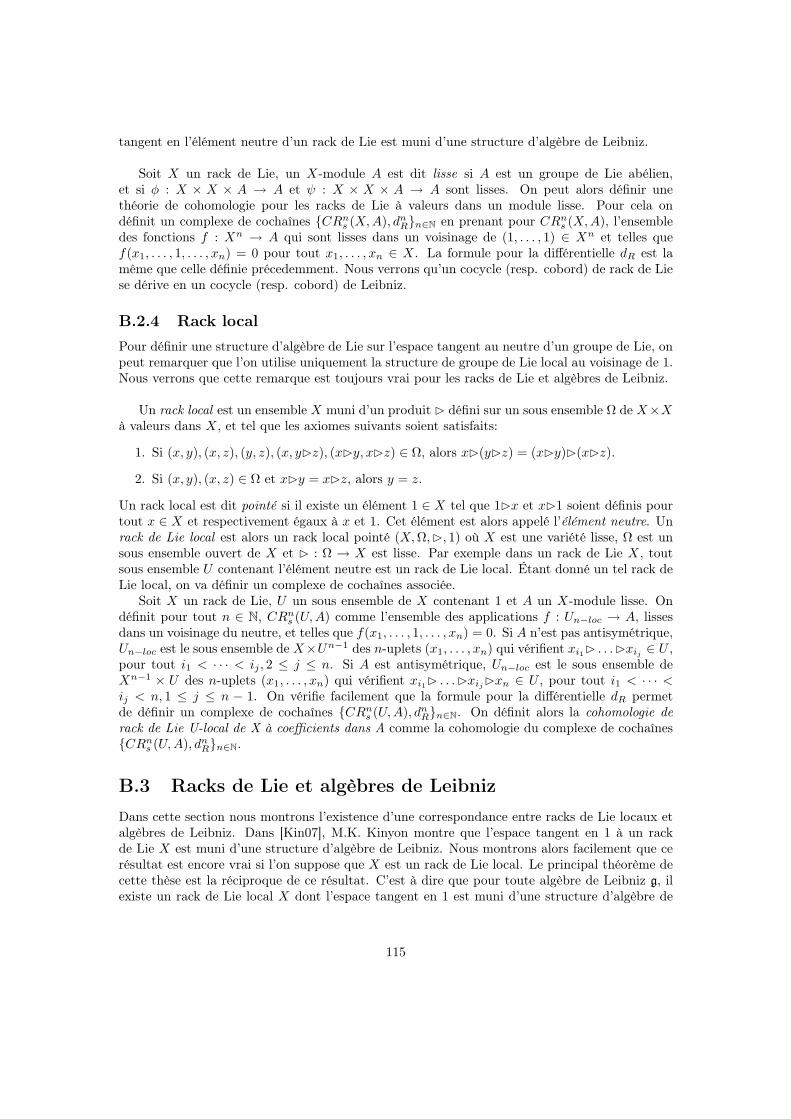
tangent en l’élément neutre d’un rack de Lie est muni d’une structure d’algèbre de Leibniz.

Soit X un rack de Lie, un X-module A est dit lisse si A est un groupe de Lie abélien,et si φ : X × X × A → A et ψ : X × X × A → A sont lisses. On peut alors définir unethéorie de cohomologie pour les racks de Lie à valeurs dans un module lisse. Pour cela ondéfinit un complexe de cochaînes CRn

s (X,A), dnRn∈N en prenant pour CRn

s (X,A), l’ensembledes fonctions f : Xn → A qui sont lisses dans un voisinage de (1, . . . , 1) ∈ Xn et telles quef(x1, . . . , 1, . . . , xn) = 0 pour tout x1, . . . , xn ∈ X. La formule pour la différentielle dR est lamême que celle définie précedemment. Nous verrons qu’un cocycle (resp. cobord) de rack de Liese dérive en un cocycle (resp. cobord) de Leibniz.

B.2.4 Rack local

Pour définir une structure d’algèbre de Lie sur l’espace tangent au neutre d’un groupe de Lie, onpeut remarquer que l’on utilise uniquement la structure de groupe de Lie local au voisinage de 1.Nous verrons que cette remarque est toujours vrai pour les racks de Lie et algèbres de Leibniz.

Un rack local est un ensemble X muni d’un produit ⊲ défini sur un sous ensemble Ω de X×Xà valeurs dans X, et tel que les axiomes suivants soient satisfaits:

1. Si (x, y), (x, z), (y, z), (x, y⊲z), (x⊲y, x⊲z) ∈ Ω, alors x⊲(y⊲z) = (x⊲y)⊲(x⊲z).

2. Si (x, y), (x, z) ∈ Ω et x⊲y = x⊲z, alors y = z.

Un rack local est dit pointé si il existe un élément 1 ∈ X tel que 1⊲x et x⊲1 soient définis pourtout x ∈ X et respectivement égaux à x et 1. Cet élément est alors appelé l’élément neutre. Unrack de Lie local est alors un rack local pointé (X,Ω,⊲, 1) où X est une variété lisse, Ω est unsous ensemble ouvert de X et ⊲ : Ω → X est lisse. Par exemple dans un rack de Lie X, toutsous ensemble U contenant l’élément neutre est un rack de Lie local. Étant donné un tel rack deLie local, on va définir un complexe de cochaînes associée.

Soit X un rack de Lie, U un sous ensemble de X contenant 1 et A un X-module lisse. Ondéfinit pour tout n ∈ N, CRn

s (U,A) comme l’ensemble des applications f : Un−loc → A, lissesdans un voisinage du neutre, et telles que f(x1, . . . , 1, . . . , xn) = 0. Si A n’est pas antisymétrique,Un−loc est le sous ensemble de X×Un−1 des n-uplets (x1, . . . , xn) qui vérifient xi1⊲ . . .⊲xij

∈ U ,pour tout i1 < · · · < ij , 2 ≤ j ≤ n. Si A est antisymétrique, Un−loc est le sous ensemble deXn−1 × U des n-uplets (x1, . . . , xn) qui vérifient xi1⊲ . . .⊲xij

⊲xn ∈ U , pour tout i1 < · · · <ij < n, 1 ≤ j ≤ n − 1. On vérifie facilement que la formule pour la différentielle dR permetde définir un complexe de cochaînes CRn

s (U,A), dnRn∈N. On définit alors la cohomologie de

rack de Lie U-local de X à coefficients dans A comme la cohomologie du complexe de cochaînesCRn

s (U,A), dnRn∈N.

B.3 Racks de Lie et algèbres de Leibniz

Dans cette section nous montrons l’existence d’une correspondance entre racks de Lie locaux etalgèbres de Leibniz. Dans [Kin07], M.K. Kinyon montre que l’espace tangent en 1 à un rackde Lie X est muni d’une structure d’algèbre de Leibniz. Nous montrons alors facilement que cerésultat est encore vrai si l’on suppose que X est un rack de Lie local. Le principal théorème decette thèse est la réciproque de ce résultat. C’est à dire que pour toute algèbre de Leibniz g, ilexiste un rack de Lie local X dont l’espace tangent en 1 est muni d’une structure d’algèbre de

115

Leibniz isomorphe à g. En fait nous montrons que le rack de Lie local intégrant g est un rack deLie local augmenté.

B.3.1 Des racks de Lie aux algèbres de Leibniz

Proposition B.3.1. Soit X un rack de Lie, alors T1X est une algebre de Leibniz.

Preuve : Soit X un rack de Lie, on note par x l’espace tangent de X en 1. La conjugaisoninduit ∀x ∈ X un automorphisme de rack de Lie cx. nous définissons ∀x ∈ X

Adx = T1cx ∈ GL(x)

et grâce à cx⊲y = cx cy c−1x et c1 = id (cf. Définition B.2.1), ceci nous donne un morphisme

de racks de LieAd : X → GL(x)

Nous pouvons différentier Ad, et nous obtenons une application linéaire

ad : X → gl(x)

Alors nous définissons un crochet [−,−] sur x = T1X en posant

[u, v] = ad(u)(v)

Maintenant, nous devons vérifier que ce crochet vérifit l’identité de Leibniz, c’est à dire

[u, [v, w]] = [[u, v], w] + [v, [u,w]]

Pour montrer cette identité, nous utilisons l’identité de rack

x⊲(y⊲z) = (x⊲y)⊲(x⊲z)

Soit u, v, w ∈ x et γu (resp. γv and γw) un chemin lisse dansX, pointé en 1, tel que∂

∂s

∣∣∣∣s=0

γu(s) =

u (resp.∂

∂s

∣∣∣∣s=0

γv(s) = v et∂

∂s

∣∣∣∣s=0

γw(s) = w). Nous avons

∂

∂t

∣∣∣∣t=0

(γu(r)⊲(γv(s)⊲γw(t))) =∂

∂t

∣∣∣∣t=0

((cγu(r) cγv(s))(γw(t))

= (Adγu(r) Adγv(s))(w)

et

∂

∂t

∣∣∣∣t=0

((γu(r)⊲γv(s))⊲(γu(r)⊲γw(t))) =∂

∂t

∣∣∣∣t=0

((cγu(r)⊲γv(s) cγu(r))(γw(t))

= (Adγu(r)⊲γv(s) Adγu(r))(w)

= (Adcγu(r)(γv(s)) Adγu(r))(w)

De plus, si nous différentions par rapport à la variable s

∂

∂s

∣∣∣∣s=0

((Adγu(r) Adγv(s))(w)) = (Adγu(r) ad(v))(w)

116

et∂

∂s

∣∣∣∣s=0

(Adcγu(r)(γv(s)) Adγu(r))(w) = (ad(Adγu(r)(v)) Adγu(r))(w)

Et si nous différentions par rapport à la variable r, nous obtenons

∂

∂t

∣∣∣∣t=0

(Adγu(r) ad(v))(w) = ad(u)(ad(v)(w))

et∂

∂r

∣∣∣∣r=0

(ad(Adγu(r)(v)) Adγu(r))(w) = ad(ad(u)(v))(w) + ad(v)(ad(u)(w))

Ainsi, par identification, nous avons l’identité de Leibniz.

Par exemple, si G est un groupe de Lie nous obtenons la structure d’algèbre de Lie canonique

sur T1G. Si Xp→ G est un rack de Lie augmenté, alors T1X

T1p→ T1G est une algèbre de Lie dans

la catégorie des applications linéaires (cf. [LP98]). Cette structure induit alors une structured’algèbre de Leibniz sur T1X.

Nous pouvons remarquer qu’une structure lisse locale au voisinage de 1 est suffisante pourmunir T1X d’une structure d’algèbre de Leibniz.

Proposition B.3.2. Soit X un rack de Lie local, alors T1X est une algèbre de Leibniz.

B.3.2 Des Asp(X)-modules aux représentations de Leibniz

Soit X un rack pointé. Un Asp(X)-module est un groupe abélien A muni d’un morphisme degroupes φ : Asp(X) → Aut(A). Par adjonction, ceci est équivalent à la donnée d’un morphismede rack pointé φ : X → Conj(Aut(A)).

Définition B.3.3. Soit X un rack de Lie, un Asp(X)-module lisse est un Asp(X)-module Atel que

1. A est un groupe de Lie abélien.

2. φ : X ×A→ A est lisse.

Rappellons que, étant donné une algèbre de Leibniz g, une g-représentation a est un espacevectoriel muni de deux applications linéaires

[−,−]L : g ⊗ a → a

et[−,−]R : a ⊗ g → a

satisfaisants les axiomes (LLM), (LML) and (MLL). (cf. la sous section B.1.2).Il y a deux classes particulières de représentations de Leibniz. La première, que nous avons

appelé symétrique, est constituée des représentations où [−,−]L = −[−,−]R. la seconde, quenous avons appelé antisymétrique, est constituée des représentations où [−,−]R = 0. Étantdonnée une algèbre de Leibniz g et a un espace vectoriel muni d’un morphisme d’algèbres de

117

Leibniz φ : g → End(a), nous pouvons définir deux structures de g-representation de Leibniz sura. Une est symétrique et définie par

[x, a]L = φx(a) and [a, x]R = −φx(a), ∀x ∈ g, a ∈ a.

et l’autre est antisymétrique et définie par

[x, a]L = φx(a) and [a, x]R = 0, ∀x ∈ g, a ∈ a.

De plus, dans la sous section B.2.2 nous avons vu que étant donné un rack (de Lie) X et Aun Asp(X)-module lisse, nous pouvons définir deux structures de X-modules (lisses) sur A. Uneest appelée symétrique et définie par

φx,y(a) = φx(a) and ψx,y(a) = a− φx⊲y(a), ∀x, y ∈ X, a ∈ A.

et l’autre est appelé antisymétrique et définie par

φx,y(a) = φx(a) and ψx,y(a) = 0, ∀x, y ∈ X, a ∈ A.

Ces deux constructions, l’une dans le monde des algèbres de Leibniz et l’autre dans le mondedes racks de Lie, sont similaires car la première est la version infinitésimale de l’autre. En effet,soit (A, φ, ψ) un X-module symétrique lisse, nous avons par définition deux applications lisses

φ : X ×X ×A→ A and ψ : X ×X ×A→ A

avec φ1,1 = id, ψ1,1 = 0. Ainsi les differentielles des deux applications au point (1, 1) nousdonnent deux applications

ǫ : X ×X → Aut(a); ǫ(x, y) = T1φx,y

etχ : X ×X → End(a);χ(x, y) = T1ψx,y

Ces applications sont lisses, donc nous pouvons les dériver au point (1, 1). Nous obtenons alorsdeux applications

T(1,1)ǫ : x ⊕ x → End(a)

etT(1,1)χ : x ⊕ x → End(a)

On pose alors[−,−]L : g ⊗ a → a; [u,m]L = T(1,1)ǫ(u, 0)(m)

et[−,−]R : a ⊗ g → a; [m,u]R = T(1,1)χ(0, u)(m)

Lemma B.3.4. L’application linéaire [−,−]L satisfait l’axiome (LLM).

Preuve : nous voulons montrer que ∀u, v ∈ x,m ∈ a

[u, [v,m]L]L = [[u, v],m]L + [v, [u,m]L]L

par hypothèse, φ satisfait la relation suivante ∀x, y, z ∈ X

φx,y⊲z φy,z = φx⊲y,x⊲z φx,z

118

et si on prend z = 1, nous obtenons

φx,1 φy,1 = φx⊲y,1 φx,1

ainsiT1φx,1 T1φy,1 = T1φx⊲y,1 T1φx,1

c’est à direǫ(x, 1) ǫ(y, 1) = ǫ(x⊲y, 1) ǫ(x, 1)

Soit u, v ∈ x and γu (resp. γv) un chemin dans X pointé en 1 tel que∂

∂s

∣∣∣∣s=0

γu(s) = u (resp.

∂

∂s

∣∣∣∣s=0

γv(s) = v). Nous avons

∂

∂t

∣∣∣∣t=0

(ǫ(γu(s), 1) ǫ(γv(t), 1)) = ǫ(γu(s), 1) ∂

∂t

∣∣∣∣t=0

ǫ(γv(t), 1)

= ǫ(γu(s), 1) [v,−]L

et

∂

∂s

∣∣∣∣s=0

(ǫ(γu(s), 1) [v, 0]L) = (∂

∂s

∣∣∣∣s=0

ǫ(γu(s), 1)) [v,−]L

= [u,−]L [v,−]L

= [u, [v,−]L]L

D’un autre côté, nous avons

∂

∂t

∣∣∣∣t=0

(ǫ(γu(s)⊲γv(t), 1) ǫ(γu(s), 1)) = [Adγu(s)(v),−]L ǫ(γu(s), 1)

et

∂

∂s

∣∣∣∣s=0

([Adγu(s)(v),−]L ǫ(γu(s), 1)) =∂

∂s

∣∣∣∣s=0

([Adγu(s)(v),−]L) ǫ(1, 1)

+ [Adγu(0)(v),−]L ∂

∂s

∣∣∣∣s=0

(ǫ(γu(s), 1))

= [[u, v],−]L + [v,−]L [u,−]L

= [[u, v],−]L + [v, [u,−]]L

Ainsi par identification[u, [v,−]L]L = [[u, v],−]L + [v, [u,−]]L

C’est à dire, [−,−]L satisfait (LLM).

Lemma B.3.5. Si (A, φ, ψ) est symétrique, alors [−,−]L = −[−,−]R et si (A, φ, ψ) est anti-symétrique, alors [−,−]R = 0.

119

Preuve : Supposons que (A, φ, ψ) est antisymétrique, alors ψ = 0, et il est clair que [−,−]R = 0.Maintenant, supposons que (A, φ, ψ) est symétrique, c’est à dire ψx,y(a) = a− φx⊲y,1(a). Nousavons χ(x, y) = T1ψx,y = id− ǫ(x⊲y, 1). Soit u ∈ x et γu un chemin dans X pointé en 1 tel que∂

∂s

∣∣∣∣s=0

γu(s) = u. Nous avons

[−, u]R = T(1,1)χ(0, u)

=∂

∂s

∣∣∣∣s=0

χ(1, γu(s))

=∂

∂s

∣∣∣∣s=0

(id− ǫ(γu(s), 1))

= −∂

∂s

∣∣∣∣s=0

ǫ(γu(s), 1)

= −[u,−]L

Finalement, nous avons montré la proposition suivante:

Proposition B.3.6. Soit X un rack de Lie, x son algebre de Leibniz, A un groupe de Lie abélienet a son algèbre de Lie. Si (A, φ, ψ) est un X-module lisse symétrique (resp. antisymétrique),alors (a, [−,−]L, [−,−]R) est un x-module symétrique (resp. antisymétrique).

B.3.3 De la cohomologie de rack de Lie à la cohomologie de Leibniz

Proposition B.3.7. Soit X un rack de Lie et A un As(X)-module lisse. Il existe des morphismesde complexes de cochaînes

CRnp (X,As)s

δn

→ CLn(x, as)

etCRn

p (X,Aa)sδn

→ CLn(x, aa)

donnés par δn(f)(a1, . . . , an) = dnf(1, . . . , 1)((a1, 0, . . . , 0), . . . , (0, . . . , 0, an)) (où dnf est la dif-férentielle n-ième de f).

Preuve : Soit f ∈ CRnp (X,As) et (x0, . . . , xn) ∈ Xn+1. Nous avons

dRf(x0, . . . , xn) =

n+1∑

i=1

(−1)i−1φx1⊲...⊲xi(f(x1, . . . , xi, . . . , xn+1))−f(x1, . . . , xi⊲xi+1, . . . , xi⊲xn+1)

(Ici φx1⊲...⊲xi= φx1⊲...⊲xi,x1⊲...⊲cx1⊲...⊲xn+1

)Soit (γ0(t0), . . . , γn(tn)) une famille de chemins γi :] − ǫi,+ǫi[→ V tels que

γi(0) = 1 et∂

∂s s=0γi(s) = xi

Nous voulons montrer queδn+1(dn

Rf) = dnL(δn(f))

Nous avons par définition

δn+1(dnRf)(a0, . . . , an) =

∂n+1

∂t0 . . . ∂tn

∣∣∣∣ti=0

df(γ0(t0), . . . , γn(tn))

120

Lemma B.3.8. ∀i ∈ 1, . . . , n

∂n+1

∂t0 . . . ∂tn

∣∣∣∣|ti=0

φγ0(t0)⊲...⊲γi(ti)(f(γ0(t0), . . . , γi−1(ti−1), γi+1(ti+1), . . . , γn(tn))) = ai.Dn(f)(a0, . . . , ai, . . . , an)

Preuve :Notation:

(t0, . . . , ti) 7→ φγ0(t0)⊲...⊲γi(ti)

sera noté par(t0, . . . , ti) 7→ A(t0, . . . , ti)

et(t0, . . . , ti, . . . , tn) 7→ f(γ0(t0), . . . , γi−1(ti−1), γi+1(ti+1), . . . , γn(tn))

sera noté par(t0, . . . , ti, . . . , tn) 7→ m(t0, . . . , ti, . . . , tn)

Nous avons

∂n+1

∂t0 . . . ∂tn

∣∣∣∣tk=0

A(t0, . . . , ti)(m(t0, . . . , tn)) =∂n

∂t0 . . . ∂tn−1

∣∣∣∣tk=0

(∂

∂tn tn=0

A(t0, . . . , ti)(m(t0, . . . , 0))

+∂n

∂t0 . . . ∂tn−1

∣∣∣∣tk=0

(A(t0, . . . , ti)(∂

∂tn

∣∣∣∣tn=0

m(t0, . . . , tn)))

=∂n

∂t0 . . . ∂tn−1

∣∣∣∣tk=0

(A(t0, . . . , ti)(∂

∂tn tn=0

m(t0, . . . , tn)))

car f(x0, . . . , 1, . . . , xn) = 0.Et par le même argument nous avons

∂n+1

∂t0 . . . ∂tn

∣∣∣∣tk=0

A(t0, . . . , ti)(m(t0, . . . , tn)) =∂

∂ti

∣∣∣∣ti=0

A(0, . . . , 0, ti)(∂n

∂t0 . . . ∂tn

∣∣∣∣tk=0

m(t0, . . . , tn))

Ainsi∂n+1

∂t0 . . . ∂tn

∣∣∣∣ti=0

A(t0, . . . , tn)(m(t0, . . . , tn)) = xi.Dn(f)(x0, . . . , xi, . . . , xn)

Lemma B.3.9. ∀i ∈ 1, . . . , n

∂n+1

∂t0 . . . ∂tn

∣∣∣∣ti=0

f(γ0(t0), . . . , γi(ti)⊲γi+1(ti+1), . . . , γi(ti)⊲γn(tn)) =

n∑

k=i+1

δnf(a0, . . . , [ai, ak], . . . , an)

Preuve : Nous avons∂n+1

∂t0 . . . ∂tn

∣∣∣∣ti=0

f(γ0(t0), . . . , γi(ti)⊲γi+1(ti+1), . . . , γi(ti)⊲γn(tn)) qui est

égal à

∂

∂ti

∣∣∣∣ti=0

dnf(1, . . . , 1)((a0, 0, . . . , 0), . . . , (0, . . . , Adγi(ti)(ai+1), . . . , 0), . . . , (0, . . . , 0, Adγi(ti)(an))

De plus, ceci est égal à

n∑

k=i+1

dnf(1, . . . , 1)((a0, 0, . . . , 0), . . . , (0, . . . , [ai, ak], . . . , 0), . . . , (0, . . . , 0, an))

121

et cette expresion est égale àn∑

k=i+1

δnf(a0, . . . , [ai, ak], . . . , an).

Donc

δn+1(dnRf)(a0, . . . , an) =

n∑

i=0

(−1)i(ai.δ

n(f)(a0, . . . , ai, . . . , an) −n∑

k=i+1

δnf(a0, . . . , [ai, ak], . . . , an))

=

n∑

i=0

(−1)iai.δn(f)(a0, . . . , ai, . . . , an) +

∑

0≤i<k≤n

(−1)i+1δnf(a0, . . . , [ai, ak], . . . , an)

c’est à direδn+1(dn

Rf) = dnL(δn(f))

La preuve est exactement la même pour le cas où A est antisymétrique.

Nous pouvons remarquer que nous n’avons besoin que d’une identité de cocycle local au voisinagede 1. Ainsi nous avons

Proposition B.3.10. Soit X un rack de Lie, U un voisinage de 1 dans X et A un As(X)-modulelisse. Nous avons des morphismes de complexes de cochaînes

CRnp (U,As)

δn

→ CLn(x, as)

etCRn

p (U,Aa)δn

→ CLn(x, aa)

donnés par δn(f)(a0, . . . , an) = dnf(1, . . . , 1)((a1, 0, . . . , 0), . . . , (0, . . . , 0, an)).

B.3.4 De la cohomologie de Leibniz vers la cohomologie de rack de Lie

local

Dans cette section, nous étudions deux cas d’intégration de cocycles de Leibniz. Cette sectionsera utilisée dans la section suivante pour intégrer toutes algèbre de Leibniz en rack de Lie localaugmenté.Premièrement, nous étudions l’intégration d’un 1-cocycle de Leibniz appartenant à ZL1(g, as) enun 1-cocycle de rack de Lie appartenant à ZR1

p(G, as)s, où G est un groupe de Lie simplement

connexe d’algèbre de Lie g et a une représentation de G.Deuxièmement, nous utilisons le résultat de la première partie pour étudier l’intégration d’un2-cocycle de Leibniz appartenant à ZL2(g, aa) en un 2-cocycle de rack de Lie local appartenant àZR2

p(U, aa)s, où U est un voisinage de 1 dans un groupe de Lie simplement connexe G d’algèbre

de Lie g, et a une représentation de G. C’est la seconde partie que nous utiliserons pour intégrerles algèbres de Leibniz.

122

Des 1-cocycles de Leibniz aux 1-cocycles de rack de Lie

Soit G un groupe de Lie simplement connexe et a une représentaiton de G. Nous voulons définirun morphisme I1 de ZL1(g, as) vers ZR1

p(G, as)s qui envoit BL1(g, as) dans BR1

p(G, as)s. Pour

ceci, nous posons

I1(ω)(g) =

∫

γg

ωeq

où ω ∈ ZL1(g, as), γ : G × [0, 1] → G est une application lisse telle que γg soit un chemin de 1à g, γ1 est le chemin constant égal à 1, et ωeq est la forme différentielle equivariante à gauchefermée appartenant à Ω1(G, a) définie par

ωeq(g)(m) = g.(ω(TgLg−1(m)))

Par définition, il est clair que I1(ω)(1) = 0.Pour le moment, I1(ω) dépend de γ, mais du fait que ω soit un cocycle, la dépendance par

rapport à γ disparait.

Proposition B.3.11. I1 ne dépend pas de γ.

Proof : Soit γ, γ′ : G× [0, 1] → G tel que γg(0) = γ′g(0) = 1 et γg(1) = γ′g(1) = g. Nous allonsmontrer que

∫

γg

ωeq =

∫

γ′g

ωeq

Nous avons∫

γgωeq −

∫γ′

gωeq =

∫γg−γ′

gωeq. Comme H1(G) = 0 et ∂(γg − γ′g) = 0, il existe

σg : [0, 1]2 → G tel que γg − γ′g = ∂σg. Donc

∫

γg

ωeq −

∫

γ′g

ωeq =

∫

γg−γ′g

ωeq

=

∫

∂σg

ωeq

=

∫

σg

ddRωeq

= 0

Ainsi I1 ne dépend pas de γ.

Proposition B.3.12. I1 envoit les cocycles sur les cocycles et les cobords sur les cobords.

123

Preuve : Premièrement, soit ω ∈ ZL1(g, as), nous avons

dRI(ω)(g, h) = g.I(ω)(h) − I(ω)(g⊲h) − (g⊲h).I(ω)(g) + I(ω)(g)

= g.

∫

γh

ωeq −

∫

γg⊲h

ωeq − (g⊲h).

∫

γg

ωeq +

∫

γg

ωeq

=

∫

γh

g.ωeq −

∫

γg⊲h

ωeq −

∫

γg

(g⊲h).ωeq +

∫

γg

ωeq

=

∫

gγh

ωeq −

∫

γg⊲h

ωeq −

∫

(g⊲h)γg

ωeq +

∫

γg

ωeq

=

∫

gγh−γg⊲h−(g⊲h)γg+γg

ωeq

Comme H1(G) = 0 et ∂(gγh − γg⊲h − (g⊲h)γg + γg) = 0, il existe γg,h : [0, 1]2 → G such that∂γg,h = gγh − γg⊲h − (g⊲h)γg + γg. Ainsi, nous avons

dRI(ω)(g, h) =

∫

∂γg,h

ωeq

=

∫

γg,h

ddRωeq

= 0

Ainsi ZL1(g, as) est envoyé dans ZR1p(G, a

s)s.

Deuxièmement, soit ω ∈ BL1(g, as). Il existe β ∈ a tel que ω(m) = m.β. Nous avons

I(ω)(g) =

∫

γg

ωeq

=

∫

γg

(dLβ)eq

=

∫

γg

ddRβeq

= βeq(g) − βeq(1)

= g.β − β

= dRβ(g)

Ainsi BL1(g, as) est envoyé dans BR1p(G, a

s)s.

Proposition B.3.13. I1 est un inverse à gauche de δ1.

Preuve : Soit ω ∈ ZL1(g, as). Soit ϕ : U → g une carte locale contenant 1 tel que ϕ(1) = 0 etdϕ−1(0) = id.Nous définissons pour x ∈ g l’application lisse αx :] − ǫ,+ǫ[→ U en posant

αx(s) = ϕ−1(sx)

124

et nous définissons, ∀s ∈] − ǫ,+ǫ[, l’application lisse γαx(s) : [0, 1] → U en posant

γαx(s)(t) = ϕ−1(tsx)

Nous avons

δ1(I1(ω))(x) =∂

∂s

∣∣∣∣s=0

I1(ω)(αx(s))

=∂

∂s

∣∣∣∣s=0

∫

γαx(s)

ωeq

=∂

∂s

∣∣∣∣s=0

∫

[0,1]

γ∗αx(s)ωeq

=∂

∂s

∣∣∣∣s=0

∫

[0,1]

ωeq(γαx(s)(t))(∂

∂t

∣∣∣∣t=0

γαx(s)(t))dt

De plus,∂

∂t

∣∣∣∣t=0

γαx(s)(t) =∂

∂t

∣∣∣∣t=0

ϕ−1(stx) = sx, donc

δ1(I1(ω))(x) =∂

∂s

∣∣∣∣s=0

∫

[0,1]

ωeq(γαx(s)(t))(sx)dt

=

∫

[0,1]

∂

∂s

∣∣∣∣s=0

ωeq(γαx(s)(t))(sx)dt

=

∫

[0,1]

∂

∂s

∣∣∣∣s=0

ωeq(ϕ−1(tsx))(sx)dt

=

∫

[0,1]

∂

∂s

∣∣∣∣s=0

(ϕ−1)∗ωeq(tsx)(sx)dt

=

∫

[0,1]

∂

∂s

∣∣∣∣s=0

s(ϕ−1)∗ωeq(tsx)(x)dt

=

∫

[0,1]

(ϕ−1)∗ωeq(0)(x)dt

= ω(x)

∫

[0,1]

dt

= ω(x)

Ainsi δ1 I1 = id

Remarque B.3.14. On peut montrer qu’il existe un isomorphisme H1(g, a)D1

→ H1s (G, a) de

la cohomologie d’algèbre de Lie vers la cohomologie de groupes de Lie (cf. [Nee04]). Nouspouvons remarquer que I1 est la même application que celle définie dans [Nee04] pour prouverla surjectivité. En fait, pour prouver la Proposition B.3.12, nous avons juste combiner le résultat

de K.H. Neeb et le fait que l’on a une injection H1s (G, a)s

id→ HR1

s(G, as).

Des 2-cocycles de Leibniz aux 2-cocycles de rack de Lie local

Soit G un groupe de Lie simplement connexe, U un voisinage de 1 dans G tel que l’applicationlog soit définie sur U et a une représentation de G. Dans la proposition (3.3.4) nous avons défini

125

pour tout n ∈ N les applications

HRns (U, aa)

[δn]−→ HLn(g, aa)

Dans la prochaine section, nous verrons qu’une algèbre de Leibniz peut être intégré en unrack de Lie local puisque [δ2] est surjectif. Plus précisemment, si nous pouvons construire uninverse à gauche pour [δ2], alors il nous donne une méthode explicite pour construire un rack deLie local qui intègre l’algèbre de Leibniz.

Dans cette section, nous définissons un morphisme [I2] de HL2(g, aa) vers HR2s(U, a

a), etnous montrons que c’est un inverse à gauche pour [δ2]. Pour construire l’application [I2], nousadaptons une méthode d’intégration des cocycles d’algèbre de Lie en cocycles de groupes de Liepar intégration sur des simplex. Cette méthode est due à W.T. Van Est ([Est54]) et utilisée parK.H. Neeb ([Nee02, Nee04]) pour le cas de la dimension infinie.

Définition de I2

Nous voulons définir une application de ZL2(g, aa) vers ZR2p(U, a

a)s telle que BL2(g, aa)soit envoyé sur BR2

p(U, aa)s. Dans la section précédente, nous avons intégré un 1-cocycle de

Leibniz sur une algebre de Lie g à coefficients dans un module symétrique as. Dans la Propo-sition (B.1.1), nous avons expliciter un morphisme entre CL2(g, aa) et CL1(g, Hom(g, a)s), quienvoit ZL2(g, aa) dans ZL1(g, Hom(g, a)s) et BL2(g, aa) dans BL1(g, Hom(g, a)s). Ainsi, nouspouvons définir une application

I : ZL2(g, aa) → ZR1p(G,Hom(g, a)s)s

qui envoit BL2(g, aa) dans BR1p(G,Hom(g, a)s)s. C’est la composée

ZL2(g, aa)τ2

→ ZL1(g, Hom(g, a)s)I1

→ ZR1p(G,Hom(g, a)s)s

Maintenant, nous voulons définir une application de ZR1p(G,Hom(g, a)s)s vers ZR2

p(U, aa). Soit

β ∈ CR1p(G,Hom(g, a)s)s, β a ces valeurs dans la représentations Hom(g, a), donc pour tout

g ∈ G, nous pouvons considérer la forme différentielle equivariante β(g)eq ∈ Ω1(G, a) définie par

β(g)eq(h)(m) := h.(β(g)(ThLh−1(m)))

Alors nous définissons un élement dans CR2p(U, a

a) en posant

f(g, h) =

∫

γg⊲h

(β(g))eq

où γ : G× [0, 1] → G est une application lisse telle que pour tout g ∈ G, γg est un chemin de 1à g dans G et γ1 = 1.Pour l’instant, un élément de ZR1

p(G,Hom(g, a)s)s n’est pas nécéssairement envoyé sur un élé-ment de ZR2

p(U, aa)s. Pour atteindre cet objectif, nous devons spécifier l’application γ, et nous

la définissons en posantγg(s) = exp(s log(g))

Alors, nous définissons I2 : ZL2(g, aa) → CR2p(U, a

a)s en posant ∀(g, h) ∈ U2−loc

I2(ω)(g, h) =

∫

γg⊲h

(I(ω)(g))eq

Par définition, il est clair que I2(ω)(g, 1) = I2(ω)(1, g) = 0.

126

Propriétés de I2

Proposition B.3.15. I2 envoit ZL2(g, aa) dans ZR2p(U, a

a)s.

Pour prouver cette proposition, nous avons besoins des lemmes suivants.

Lemma B.3.16. Pour tout (g, h) ∈ U2−loc, nous avons γg⊲h = g⊲γh.

Preuve : Soit (g, h) ∈ U2−loc, par définition nous avons

γg⊲h(s) = exp(s(log(g⊲h)))

Par naturalité de l’exponentielle, et a fortiori du logarithme, nous avons

exp(s(log(g⊲h))) = exp(sAdg(log(h)))

= exp(Adg(s log(h)))

= cg(exp(s log(h)))

= cg(γh(s))

Ainsi γg⊲h = g⊲γh.

Lemma B.3.17. Soit G un groupe de Lie, a une représentation de G et ω ∈ Hom(g, a). Nousavons ∀g ∈ G

g.(ωeq) = c∗g((g.ω)eq)

Preuve : Sot g, h ∈ G, x ∈ ThG, nous avons:

(c∗g((g.ω)eq))(h)(x) = (g.ω)eq(g⊲h)(dhcg(x))

= (g⊲h).(g.ω)(dg⊲hLg⊲h−1(dhcg(x)))

= (g⊲h).(g.ω)(dh(cg Lh−1)(x))

= (g⊲h).(g.(ω(Ad(g−1)(dh(cg Lh−1)(x)))))

= gh.(ω(dh(cg−1 cg Lh−1)(x)))

= g.(h.(ω(dhLh−1(x))))

= g.(ωeq(h)(x))

Ainsi c∗g((g.ω)eq) = g.(ω)eq.

Preuve de la proposition : Soit ω ∈ ZL2(g, aa) et (g, h, k) ∈ U3−loc. Nous avons

dR(I2(ω))(g, h, k) = g.I2(ω)(h, k) − I2(ω)(g⊲h, g⊲k) − (g⊲h).I2(ω)(g, k) + I2(ω)(g, h⊲k)

= g.

∫

γh⊲k

(I(ω)(h))eq −

∫

γg⊲(h⊲k)

(I(ω)(g⊲h))eq − (g⊲h).

∫

γg⊲k

(I(ω)(g))eq

+

∫

γg⊲(h⊲k)

(I(ω)(g))eq

=

∫

γh⊲k

g.((I(ω)(h))eq) −

∫

γg⊲(h⊲k)

(I(ω)(g⊲h))eq −

∫

γg⊲k

(g⊲h).((I(ω)(g))eq)

+

∫

γg⊲(h⊲k)

(I(ω)(g))eq

127

Grâce au Lemma B.3.17, nous avons

dR(I2(ω))(g, h, k) =

∫

γh⊲k

c∗g((g.I(ω)(h))eq) −

∫

γg⊲(h⊲k)

I(ω)(g⊲h)eq −

∫

γg⊲k

c∗g⊲h(((g⊲h).I(ω)(g))eq)

+

∫

γg⊲(h⊲k)

I(ω)(g)eq

=

∫

cgγh⊲k

(g.I(ω)(h)eq −

∫

γg⊲(h⊲k)

I(ω)(g⊲h)eq −

∫

cg⊲hγg⊲k

((g⊲h).I(ω)(g))eq

+

∫

γg⊲(h⊲k)

I(ω)(g)eq

et grâce au Lemma B.3.16, nous avons

dR(I2(ω))(g, h, k) =

∫

γg⊲(h⊲k)

(g.I(ω)(h))eq −

∫

γg⊲(h⊲k)

I(ω)(g⊲h)eq −

∫

γg⊲(h⊲k

((g⊲h).I(ω)(g))eq

+

∫

γg⊲(h⊲k)

I(ω)(g)eq

=

∫

γg⊲(h⊲k)

(g.I(ω)(h))eq − I(ω)(g⊲h)eq − ((g⊲h).I(ω)(g))eq + I(ω)(g)eq

=

∫

γg⊲(h⊲k)

(g.I(ω)(h) − I(ω((g⊲h) − (g⊲h).I(ω)(g) + I(ω)(g))eq

=

∫

γg⊲(h⊲k)

dR(I(ω))(g, h)

= 0

Ainsi ZL2(g, aa) est envoyé dans ZR2p(U, a

a)s.

Proposition B.3.18. I2 envoit BL2(g, aa) dans BR2p(U, a

a)s

Preuve : Soit ω ∈ BL2(g, aa), il existe un élément β ∈ CL1(g, aa) tel que ω = dLβ. Nous avons

I(ω)(g) = I1(τ2(ω))(g)

=

∫

γg

(τ2(ω))eq

=

∫

γg

(τ2(dLβ))eq

Le fait que τnn∈N est un morphisme de complexe de cochaînes implique que

I(ω)(g) =

∫

γg

(d(τ1(β)))eq

=

∫

γg

ddR((τ1(β))eq)

=

∫

∂γg

(τ1(β))eq

= g.β − β

128

Ainisi pour (g, h) ∈ U2−loc nous avons en utilisant le Lemma B.3.17

I2(ω)(g, h) =

∫

γg⊲h

(I(ω)(g))eq

=

∫

γg⊲h

((g.β) − β)eq

=

∫

γg⊲h

(g.β)eq −

∫

γg⊲h

βeq

=

∫

γg⊲h

(c∗g−1(g.(βeq))) −

∫

γg⊲h

βeq

=

∫

cg−1γg⊲h

g.(βeq) −

∫

γg⊲h

βeq

= g.

∫

cg−1γg⊲h

βeq −

∫

γg⊲h

βeq

= g.

∫

γh

βeq −

∫

γg⊲h

βeq

= dR(I1(β))(g, h)

Ainsi BL2(g, aa) est envoyé dans BR2p(U, a)s.

Proposition B.3.19. I2 est un inverse à gauche pour δ2.

Preuve : Soit x, y ∈ g, et Ix (resp. Iy) un intervalle dans R tel que ǫx(s) = exp(sx) (resp.ǫy(s) = exp(sy)) soit défini ∀s ∈ Ix (resp. ∀s ∈ Iy). L’application ǫx⊲ǫy : Ix × Iy → G estcontinue, donc il existe W un sous ensemble ouvert de Ix × Iy tel que (ǫx⊲ǫy)(W ) ⊆ U . Ainsi,il existe un intervalle J ⊆ Ix ∩ Iy tel que ǫx(s)⊲ǫy(t) ∈ U ∀(s, t) ∈ J × J .

Nous devons montrerδ2 I2 = id

Soit ω ∈ ZL2(g, aa). Par définition, nous avons

δ2(I2(ω))(x, y) =∂2

∂s∂t

∣∣∣∣|s,t=0

I2(ω)(ǫx(s), ǫy(s))

=∂2

∂s∂t

∣∣∣∣|s,t=0

∫

γǫx(s)⊲ǫy(t)

(I(ω)(ǫx(s)))eq

=∂

∂s

∣∣∣∣|s=0

(∂

∂t

∣∣∣∣|t=0

∫

γǫy(t)

c∗ǫx(s)(I(ω)(ǫx(s)))eq)

Premièrement, nous calculons

∂

∂t

∣∣∣∣|t=0

∫

γǫy(t)

c∗ǫx(s)(I(ω)(ǫx(s)))eq

129

Par souci de clarté, nous posons α = c∗ǫx(s)(I(ω)(ǫx(s)))eq and βt = γǫy(t). Nous avons

∂

∂t

∣∣∣∣|t=0

∫

β

α =∂

∂t

∣∣∣∣|t=0

∫

[0,1]

β∗α

=∂

∂t

∣∣∣∣|t=0

∫

[0,1]

ft(r)dr

=

∫

[0,1]

∂

∂t

∣∣∣∣|t=0

ft(r)dr

où ft(r) = α(βt(r))(β′t(r)).

Nous avons

∂

∂t

∣∣∣∣|t=0

ft(r) = (∂

∂t

∣∣∣∣|t=0

α(βt(r)))β′0(r) + (α(β0(r)))(

∂

∂t

∣∣∣∣|t=0

β′t(r))

De plus, nous avonsα(β0(r)) = α(1)

β′0(r) = 0

et∂

∂t

∣∣∣∣|t=0

β′t(r) = y

Donc nous avons∂

∂t

∣∣∣∣|t=0

∫

β

α =

∫

[0,1]

α(1)(x)dr = α(1)(y)

et

δ2(I2(ω))(x, y) =∂

∂s

∣∣∣∣|s=0

(c∗ǫx(s)(I(ω)(ǫx(s)))eq)(1)(y)

nous avons de plus

c∗ǫx(s)(I(ω)(ǫx(s))eq)(1)(y) = (I(ω)(ǫx(s)))eq(cǫx(s)(1))(Adǫx(s)(y))

= I(ω)(ǫx(s))(Adǫx(s)(y))

= (

∫

γǫx(s)

τ2(ω)eq)(Adǫx(s)(y))

Si l’on pose∫

γǫx(s)τ2(ω)eq = σ(s) and Adǫx(s)(y) = λ(s), nous avons

∂

∂s

∣∣∣∣|s=0

((

∫

γǫx(s)

τ2(ω)eq)(Adǫx(s)(y))) =∂

∂s

∣∣∣∣|s=0

σ(s)(λ(s))

= σ′(0)(λ(0)) + σ(0)(λ′(0))

Nous avonsσ(0) = 0

λ(0) = y

130

etσ′(0) = τ2(ω)(x)

Donc∂

∂s

∣∣∣∣|s=0

((

∫

γǫx(s)

τ2(ω)eq)(Adǫx(s)(y))) = τ2(ω)(x)(y)

Ainsi δ2(I2(ω))(x, y) = ω(x, y).

Remarque B.3.20. Supposons que nous ayons un 2-cocycle de Leibniz ω qui soit aussi un2-cocycle de Lie. Dans ce cas, nous pouvons intégrer ω cocycle de rack de Lie local, mais aussien un cocycle de groupe de Lie local (cf. Lemma 5.2 p.18 dans [Nee04]). Il est alors naturel dese demander si les deux constructions sont reliées l’une à l’autre.

Proposition B.3.21. Soit G un groupe de Lie, g son algèbre de Lie, a une représentation deG, ω ∈ Λ2(g, a) et γ1, γ2 des chemins lisses de G pointé en 1. Alors

∫

γ1

( ∫

γ2

(τ2(ω))eq)eq

=

∫

γ1γ2

ωeq

où γ1γ2 : [0, 1]2 → G; (s, t) 7→ γ1(t)γ2(s).

Preuve : D’une part, nous avons∫

γ1γ2

ωeq =

∫

[0,1]2(γ1γ2)

∗ωeq

=

∫

[0,1]2ωeq(γ1γ2)(

∂

∂sγ1(t)γ2(s),

∂

∂tγ1(t)γ2(s))dsdt

et cette expression est égale à∫

[0,1]2γ1(t)γ2(s).ω

(dγ2(s)Lγ2(s)−1(

∂

∂sγ2(s)), Adγ2(s)−1(dγ1(t)Lγ1(t)−1(

∂

∂tγ1(t)))

)(B.4)

D’autre part, nous avons∫

γ1

( ∫

γ2

(τ2(ω))eq)eq

=

∫

[0,1]

γ∗1 (

∫

γ2

(τ2(ω)eq)eq)

=

∫

[0,1]

(

∫

γ2

(τ2(ω))eq)eq(γ1(t))(∂

∂tγ1(t))dt

=

∫

[0,1]

γ1(t).(

∫

γ2

(τ2(ω))eq)(dγ1(t)Lγ1(t)−1(∂

∂tγ1(t)))dt

=

∫

[0,1]

γ1(t).(

∫

[0,1]

(τ2(ω))eq(γ2(s))(∂

∂sγ2(s)))(dγ1(t)Lγ1(t)−1(

∂

∂tγ1(t)))dt

Cette expression est égale à∫

[0,1]

γ1(t).(

∫

[0,1]

γ2(s).(τ2(ω))(dγ2(s)Lγ2(s)−1(

∂

∂sγ2(s)))ds)(dγ1(t)Lγ1(t)−1(

∂

∂tγ1(t)))dt

131

qui est égale à∫

[0,1]

γ1(t).(

∫

[0,1]

γ2(s).ω(dγ2(s)Lγ2(s)−1(∂

∂sγ2(s)), Adγ2(s)−1(·))ds)(dγ1(t)Lγ1(t)−1(

∂

∂tγ1(t)))dt

En utilisant le théorème de Fubini, nous montrons alors que cette expression est égale à (B.4).

Si nous appliquons ce résultat au cas où γ1(s) = γg⊲h(s) = exp(s log(g⊲h)) et γ2(s) = γg(s) =exp(s log(g)) pour (g, h) ∈ U2−loc, nous obtenons alors

Corollaire B.3.22. Si ω ∈ ZL2(g, aa)∩Z2(g, a), alors I2(ω)(g, h) = ι2(ω)(g, h)− ι2(ω)(g⊲h, g)où ι2(ω)(g, h) =

∫σg,h

ωeq est un 2-cocycle de groupe de Lie local (cf. Lemma 5.2 p.18 dans

[Nee04]).

Nous pouvons remarquer que I2 est plus qu’un cocycle de rack de Lie local. Précisement, siω est dans ZL2(g, aa) alors l’identité de cocycle de rack de Lie local satisfaite par I2(ω), provientd’une autre identité satisfaite pas I2(ω). En effet, l’application I2 est définie en utilisant I, etpour vérifier que I2 envoit les cocycles de Leibinz dans les cocycles de rack local, nous avonsutilisé la Proposition B.3.12. Cette proposition établit que I1 envoit les cocycles de Lie dans lescocycles de rack. Mais nous avons remarqué dans la Remarque B.3.14 que l’identité de cocyclede rack satisfaite par I1(ω), provient de l’identité de cocycle de groupe. Ainsi, il est naturel depenser que nous avons oublier de la structure sur I2(ω). La proposition suivante explique quelleest l’identité satisfaite par I2(ω) induisant l’identité de rack local.

Proposition B.3.23. Si ω ∈ ZL2(g, aa), alors I2(ω) satisfait l’identité

g.I2(ω)(h, k) − I2(ω)(gh, k) + I2(ω)(g, h⊲k) = 0, ∀(g, h, k) ∈ U3−loc

De plus, cette identité induit l’identité de cocycle de rack local.

Preuve : Soit ω ∈ ZL2(g, aa) et (g, h, k) ∈ U3−loc nous avons:

g.I2(ω)(h, k) − I2(ω)(gh, k) + I2(ω)(g, h⊲k) = g.

∫

γh⊲k

(I(ω)(h))eq −

∫

γ(gh)⊲k

(I(ω)(gh))eq

+

∫

γg⊲(h⊲k)

(I(ω)(g))eq

=

∫

γh⊲k

g.((I(ω)(h))eq) −

∫

γg⊲(h⊲k)

(I(ω)(gh))eq

+

∫

γg⊲(h⊲k)

(I(ω)(g))eq

=

∫

γh⊲k

c∗g((g.I(ω)(h))eq) −

∫

γg⊲(h⊲k)

(I(ω)(gh))eq

+

∫

γg⊲(h⊲k)

(I(ω)(g))eq

132

g.I2(ω)(h, k) − I2(ω)(gh, k) + I2(ω)(g, h⊲k) =

∫

cgγh⊲k

(g.I(ω)(h))eq −

∫

γg⊲(h⊲k)

(I(ω)(gh))eq

+

∫

γg⊲(h⊲k)

(I(ω)(g))eq

=

∫

γg⊲(h⊲k)

(g.I(ω)(h))eq −

∫

γg⊲(h⊲k)

(I(ω)(gh))eq

+

∫

γg⊲(h⊲k)

(I(ω)(g))eq

=

∫

γg⊲(h⊲k)

(g.I(ω)(h))eq − (I(ω)(gh))eq + I(ω)(g)eq

=

∫

γg⊲(h⊲k)

(g.I(ω)(h) − I(ω)(gh) + I(ω)(g))eq

=

∫

γg⊲(h⊲k)

d(I(ω))(g, h)

= 0

Ainsi I2(ω) satisfait l’identité voulue.De plus, soit (g, h, k) ∈ U3−loc, nous avons

dR(I2(ω))(g, h, k) = g.(I2(ω)(h, k)) − I2(ω)(g⊲h, g⊲k) − (g⊲h).I2(ω)(g, k) + I2(ω)(g, h⊲k)

= g.(I2(ω)(h, k)) − I2(ω)(g⊲h, g⊲k) − (g⊲h).I2(ω)(g, k) + I2(ω)(g, h⊲k)

− I2(ω)(gh, k) + I2(ω)(gh, k)

=(g.(I2(ω)(h, k)) − I2(ω)(gh, k) + I2(ω)(g, h⊲k)

)

−((g⊲h).I2(ω)(g, k) − I2(ω)(gh, k) + I2(ω)(g⊲h, g⊲k)

)

= 0 − 0

= 0

Ainsi I2(ω) est un cocycle de rack de Lie local.

Nous verrons dans la prochaine section que cette identité permet d’intégrer toutes algèbres deLeibniz en un rack de Lie local augmenté.

B.3.5 Des algèbres de Leibniz aux racks de Lie locaux

Dans cette section, nous exposons le théorème principale de notre thèse. Dans la PropositionB.3.1 nous avons vu que l’espace tangent en 1 d’un rack de Lie (local) est muni d’une structured’algèbre de Leibniz. Réciproquement, nous montrons que toutes algèbres de Leibniz peut êtreintégré en un rack de Lie local augmenté. Notre construction est explicite, et par cette construc-tion, une algèbre de Lie est intégré en un groupe de Lie. Réciproquement, nous montrons qu’unrack de Lie local augmenté dont l’espace tangent en 1 est une algèbre de Lie est nécéssairementun groupe de Lie (local). C’est à dire qu’il existe une structure de groupe de Lie sur le rack deLie local augmenté, et la conjugaison sur le rack de Lie local augmenté est la conjugaison dugroupe.

133

L’idée de la preuve est simple et utilise la connaissance du troisième théorème de Lie. Soit g

une algèbre de Leibniz. Tout d’abord, nous décomposons l’espace vectoriel g en la somme directed’algèbres de Leibniz g0 et a que nous savons intégrer. Comme nous connaissons le théorèmepour les algèbres de Lie, c’est le cas si g est une extension abélienne d’une algèbre de Lie g0 parune g0-representation a. Ainsi, g est isomorphe à a ⊕ω g0. l’algèbre de Leibniz a est abélienne,donc s’intègre en a, et g0 est une algèbre de Lie, donc s’intègre en un groupe de Lie simplementconnexe G0. Maintenant, nous devons comprendre comment recoller a et G0. C’est à dire, nousdevons comprendre comment la donnée du recollement ω s’intègre en en une donnée de recolle-ment f entre a et G0. C’est le cocycle de rack de Lie local I2(ω), construit dans la sectionprécédente, qui répond à cette question. Ainsi, nous avons montré qu’une algèbre de Leibniz g

s’intègre en un rack de Lie local de la forme a ×f G0.

Soit g une algèbre de Leibniz, il y a plusieurs façons de voir g comme une extension abélienned’une algèbre de Lie g0 par une g0-représentation a. Ici, nous prenons l’extension abélienneassociée au centre (à gauche) de g. Par définition, le centre (à gauche) est

ZL(g) = x ∈ g | [x, y] = 0 ∀y ∈ g

ZL(g) est un idéal de g et nous pouvons considérer le quotient de g par ZL(g). C’est une algèbrede Leibniz, et plus précisemment une algèbre de Lie car gann est inclu dans ZL(g). Nous notons cequotient par g0. Ainsi, pour une algèbre de Leibniz g, il existe une extension abélienne canoniquedonnée par

ZL(g)i→ g

p։ g0

Cette extension donne une structure de g0-représentation à ZL(g), et par définition de ZL(g),cette représentation est antisymétrique. Cette classe d’équivalence est caractérisée par une classede cohomologie dans HL2(g0, ZL(g)). Ainsi il existe un élément ω ∈ ZL2(g0, ZL(g)) tel que

l’extension ZL(g)i→ g

p։ g0 soit équivalente à

ZL(g)i→ g0 ⊕ω ZL(g)

π։ g0

g0 est une algèbre de Lie, donc s’intègre en un groupe de Lie connexe et simplement connexeG0, et ZL(g) est une algèbre de Lie abélienne, donc s’intègre en elle même. ZL(g) est uneg0-représentation de Lie et G0 est simplement connexe, donc par le second théorème de LieZL(g) est un G0-module lisse. Ainsi ZL(g) est muni d’une structure de G0-module (de rack)antisymétrique lisse. Le cocycle ω ∈ ZL2(g, ZL(g)) s’intègre en un cocycle de rack de Lie localI2(ω) ∈ ZR2

p(G0, ZL(g))s, et nous pouvons poser une structure de rack de Lie local sur le produitcartésien G0 × ZL(g) en posant

(g, a)⊲(h, b) = (g⊲h, φg,h(b) + ψg,h(a) + I2(ω)(g, h))

où φg,h(b) = g.b et ψg,h(a) = 0. C’est à dire nous avons

(g, a)⊲(h, b) = (g⊲h, g.b+ I2(ω)(g, h)))

Par construction il est clair que ce rack de Lie local a son espace tangent en 1 muni d’unestructure d’algèbre de Leibniz isomorphe à g. Finalement, nous avons montré la propositionsuivante

Théorème B.3.24. Toute algèbre de Leibniz g s’intègre en un rack de Lie local de la forme

G0 ×I2(ω) aa

134

avec pour conjugaison

(g, a)⊲(h, b) = (g⊲h, g.b+ I2(ω)(g, h)) (B.5)

et élément neutre (1, 0), où G0 est une groupe de Lie, a un G0-module et ω ∈ ZL2(g0, aa).

Réciproquement, l’espace tangent en 1 d’un rack de Lie local de cette forme est muni d’unestructure d’algèbre de Leibniz.

Nous demandons plus dans notre problème de départ. En effet, nous demandons en plusqu’une algèbre de Lie s’intègre en un groupe de Lie. Ainsi, quand g est une algèbre de Lie, nousdevons montrer que G0×ZL(g) est muni d’une structure de groupe de Lie telle que la conjugaisonsur G0 ×I2(ω) ZL(g) soit induit par le produit de rack sur Conj(G0 × ZL(g)).

Soit g une algèbre de Lie, le centre à gauche ZL(g) est égal au centre Z(g). L’extension

abélienne ZL(g)i→ g

p։ g0 munit ZL(g) avec une structure antisymétrique mais aussi une

structure symétrique, donc une structure triviale. Cette extension devient une extension centraleet le cocycle ω ∈ ZL2(g0, Z(g)) est aussi dans Z2(g0, Z(g)). D’une part, avec ω nous pouvonsconstruire un cocycle de rack de Lie local I2(ω), et d’autre part, nous pouvons construire uncocycle de groupe de Lie ι2(ω). In (3.4.12), nous avons montré que I2(ω)(g, h) = ι2(ω)(g, h) −ι2(ω)(g⊲h, g) pour tout (g, h) ∈ U2loc. Ainsi, la conjugaison dans G0×I2(ω)Z(g) peut être écrite

(g, a)⊲(h, b) = (g⊲h, I2(ω)(g, h)) = (g⊲h, ι2(ω)(g, h) − ι2(ω)(g⊲h, g)).

Cette formule est celle de la conjugaison dans le groupe G0 ×ι2(ω) Z(g), où le produit est définipar

(g, a)(h, b) = (gh, ι2(g, h))

Réciproquement, supposons qu’un rack de Lie de la forme G0 ×I2(ω) aa a son espace tangenten 1, g0⊕ωaa, muni d’une structure d’algèbre de Lie. Nécessairement, a est une g0-representationtriviale et ω ∈ Z2(g0, a). Ainsi, comme avant, I2(ω)(g, h) = ι2(ω)(g, h)−ι2(ω)(g⊲h, g) pour tout(g, h) ∈ U2−loc et la conjugaison définie par (B.5) est induite par la conjugaison venant de lastructure de groupe sur G0 ×ι2(ω) a. Finalement, nous avons le théorème suivant

Théorème B.3.25. Toute algèbre de Leibniz g s’intègre en un rack de Lie local de la forme

G0 ×I2(ω) aa

avec pour conjugaison

(g, a)⊲(h, b) = (g⊲h, g.b+ I2(ω)(g, h)) (B.6)

et élément neutre (1, 0), où G0 est un groupe de Lie, a une représentation de G0 et ω ∈ZL2(g0, a

a). Réciproquement, l’espace tangent en 1 d’un rack de Lie local de cette forme estmuni d’une structure d’algèbre de Leibniz.

De plus, dans le cas spécial où g est une algèbre de Lie, la construction ci-dessus munieG0 ×I2(ω) aa d’un produit de rack provenant de la conjugaison dans un groupe de Lie. Récipro-quement, si l’espace tangent en 1 de G0 ×I2(ω) aa est une algèbre de Lie, alors G0 ×I2(ω) aa peutêtre muni d’une structure de groupe de Lie, et la conjugaison induite par la structure de groupede Lie est celle définie par (B.6).

135

Des algèbres de Leibniz aux rack de Lie augmentés locaux

Soit g0 une algèbre de Lie, a une g-représentation et ω ∈ ZL2(g0, aa). Dans (3.4.5), nous avons

montré que I2(ω) est un cocycle de rack de Lie local. Nous avons aussi montré qu’il satisfaitl’identité

g.I2(ω)(h, k) − I2(ω)(gh, k) + I2(ω)(g, h⊲k) = 0 (B.7)

for all (g, h, k) ∈ U3−loc.

La question naturelle est alors : Quelle structure algébrique sur G0×I2(ω) aa est encodé par cetteidentité?

Définition B.3.26. Soit G un groupe. Un G-ensemble local est un ensemble X muni d’uneapplication ρ définie sur un sous ensemble Ω de G ×X à valeurs dans X telle que les axiomessuivants soient satisfaits

1. Si (h, x), (gh, x), (g, ρ(h, x)) ∈ Ω, alors ρ(g, ρ(h, x)) = ρ(gh, x).

2. ∀x ∈ X, (1, x) ∈ Ω et ρ(1, x) = x.

Un G-ensemble lisse est une variété lisse X munie d’une structure de G-ensemble local vérifiant

1. Ω est un sous ensemble ouvert de X ×X.

2. ρ : Ω → X est lisse.

Un point fixe est un élément x0 ∈ X tel que ∀g ∈ G, (g, x0) ∈ Ω et ρ(g, x0) = x0.

Dans la proposition suivante, nous montrons que l’identité (B.7) munit G0 ×I2(ω) aa d’unestructure de G0-ensemble local.

Proposition B.3.27. G0 ×I2(ω) aa est un G0-ensemble local lisse, et (1, 0) est un point fixe.

Preuve : Nous définissons un sous ensemble ouvert Ω et une application lisse ρ par

1. Ω = (g, (h, b)) ∈ G0 × (G0 ×I2(ω) aa)|(g, h) ∈ U2−loc.

2. ρ(g, (h, b)) = (g⊲h, g.b+ I2(ω)(g, h)).

Soit (h, (k, z)), (gh, (k, z)), (g, ρ(h, (k, z))) ∈ Ω. Ceci est équivalent à la condition (h, k), (gh, k), (g, h⊲k) ∈U2−loc, c’est à dire (g, h, k) ∈ U3−loc. Nous avons

ρ(g, ρ(h, (k, z))) = ρ(g, (h⊲k, h.z + I2(ω)(h, k)))

= (g⊲(h⊲k), g.(h.z) + g.I2(ω)(h, k) + I2(ω)(g, h⊲k))

En utilisant les identités (2) et (gh)⊲k = g⊲(h⊲k), nous avons

ρ(g, ρ(h, (k, z))) = ((gh)⊲k, (gh).z + I2(ω)(gh, k))

= ρ(gh, ρ(k, z))

Donc ρ(g, ρ(h, (k, z))) = ρ(gh, ρ(k, z)).De plus, nous avons ρ(1, (k, z)) = (1⊲k, 1.z + I2(ω)(1, k)) = (k, z) et ρ(g, (1, 0)) = (g⊲1, g.0 +I2(ω)(g, 1)) = (1, 0). Ainsi G0 ×I2(ω) aa est un G0-ensemble local lisse et (1, 0) est un point fixepour cette action local.

136

Nous pouvons remarquer que l’on peut reconstruire le produit de rack sur G0 ×I2(ω) aa à partirde la formule de l’action de G0. En effet, nous avons

(g, a)⊲(h, b) = g.(h, b) = p(g, a).(h, b)

où p est la projection sur le premier facteur G0 ×I2(ω) aap։ G0. De plus, p(1, 0) = 1 et p est

équivariant. En effet, soit (g, (h, y)) ∈ Ω, nous avons p(ρ(g.(h, y))) = p(g⊲h, g.y+ I2(ω)(g, h)) =g⊲h = g.p(h, y). Ainsi nous avons montré la proposition suivante

Proposition B.3.28. G0 ×I2(ω) aap։ G0 est un rack de Lie augmenté local.

Ainsi nous pouvons réécrire notre théorème principal

Théorème B.3.29. Toute algèbre de Leibniz g s’intègre en un rack de Lie augmenté local de laforme

G0 ×I2(ω) aap։ G0

avec action localg.(h, b) = (g⊲h, g.b+ I2(ω)(g, h))

et élément neutre (1, 0), où G0 est un groupe de Lie, a une représentation de G0 et ω ∈ZL2(g0, a

a). Réciproquement, l’espace tangent en 1 d’un rack de Lie augmenté local de cetteforme est muni d’une structure d’algèbre de Leibniz.

De plus, dans le cas spécial où g est une algèbre de Lie, la construction ci-dessus munieG0 ×I2(ω) aa d’un produit de rack provenant de la conjugaison dans un groupe de Lie. Récipro-quement, si l’espace tangent en 1 de G0 ×I2(ω) aa est une algèbre de Lie, alors G0 ×I2(ω) aa peutêtre muni d’une structure de groupe de Lie, et la conjugaison induite par la structure de groupede Lie est celle définie par (B.6).

B.3.6 Exemples d’intégration d’algèbres de Leibniz non scindées

En dimension 4

Exemple B.3.30. Soit g = R4. Nous définissons une application linéaire g par

[e1, e1] = e4

[e1, e2] = e4

[e2, e1] = −e4

[e2, e2] = e4

[e3, e3] = e4

et tous les crochets des autres combinaisons d’éléments de la base égaux à zéro. Nous avons

[(x1, x2, x3, x4), (y1, y2, y3, y4)] = (0, 0, 0, x1y1 + x1y2 − x2y1 + x2y2 + x3y3)

Proposition B.3.31. (g, [−,−]) est une algèbre de Leibniz.

Preuve : Nous avons

[(x1, x2, x3, x4), [(y1, y2, y3, y4), (z1, z2, z3, z4)]] = (0, 0, 0, 0)

137

et[(y1, y2, y3, y4), [(x1, x2, x3, x4), (z1, z2, z3, z4)]] = (0, 0, 0, 0)

et[[(x1, x2, x3, x4), (y1, y2, y3, y4)], (z1, z2, z3, z4)] = (0, 0, 0, 0)

Ainsi le crochet [−,−] satisfait l’identité de Leibniz.

Pour suivre la construction expliquée ci-dessus, nous devons déterminer le centre à gauche ZL(g),le quotient de g par ZL(g) noté g0, l’action de g0 sur ZL(g) et le 2-cocycle de Leibniz décrivantl’extension abélienne ZL(g) → g ։ g0.

Soit x ∈ ZL(g), pour y = (1, 0, 0, 0), y = (0, 1, 0, 0) ou y = (0, 0, 1, 0) dans g, nous avons[x, y] = 0. Ceci implique que x1 = x2 = x3 = 0. Réciproquement, tout élément dans g ayant lestrois premières coordonnées égales à 0 est dans ZL(g). Ainsi ZL(g) =< e4 > et g0 ≃< e1, e2, e3 >.Le crochet sur g0 est égal à zéro, donc g0 est une algèbre de Lie abélienne. L’action de g0 surZL(g) est donnée par

ρx(y) = [(x1, x2, x3, 0), (0, 0, 0, y4)] = (0, 0, 0, 0)

et le 2-cocycle de Leibniz est donné par

ω(x, y) = [(x1, x2, x3, 0), (y1, y2, y3, 0)] = (0, 0, 0, x1y1 + x1y2 − x2y1 + x2y2 + x3y3)

Maintenant, nous devons déterminer le groupe de Lie G0 associé à g0, l’action de G0 surZL(g) intégrant ρ et le cocycle de rack de Lie intégrant ω.

g0 est une algèbre de Lie abélienne, donc un groupe de Lie intégrant g0 est G0 = g0. De plusla représentation ρ est nulle, donc l’action de groupe de Lie de G0 sur ZL(g) qui intègre ρ estl’action triviale. Du fait que ρ soit nulle et g0 abélienne, la différentielle d1

L : CL1(g0, ZL(g)) →CL2(g0, ZL(g)) est nulle. Ainis, du fait que gann = ZL(g), g est non scindée. Ce qu’il reste àtraiter est l’intégration du cocycle ω. Une formule pour f , un cocycle de rack de Lie intégrantω, est

f(a, b) =

∫

γb

(

∫

γa

τ2(ω)eq)eq

où γa(s) = sa et γb(t) = tb. Soit a ∈ G0 and x, y ∈ g0. Nous avons

∫

γa

τ2(ω)eq =

∫

[0,1]

τ2(ω)eq(γa(s))(∂

∂s

∣∣∣∣s=0

γa(s))ds

=

∫

[0,1]

Φγa(s)(τ2(ω)(a))ds

=

∫

[0,1]

τ2(ω)(a)ds

= τ2(ω)(a)

138

Donc

f(a, b) =

∫

γb

(τ2(ω)(a))eq

=

∫

[0,1]

γ∗b (τ2(ω)(a))eq

=

∫

[0,1]

τ2(ω)(a))eq(γb(t))(∂

∂t

∣∣∣∣t=0

γb(t))dt

=

∫

[0,1]

τ2(ω)(a))(b)dt

= τ2(ω)(a)(b)

= ω(a, b)

Ainsi, la conjugaison dans G0 ×f ZL(g) = R4 est donnée par

(a1, a2, a3, a4)⊲(b1, b2, b3, b4) = (b1, b2, b3, a1b1 + a2b2 + a3b3 + a1b2 − a2b1 + b4)

nous avons

∂2

∂s∂t |s,t=0(sa1, sa2, sa3, sa4)⊲(tb1, tb2, tb3, tb4) =

∂2

∂s∂t |s,t=0(tb1, tb2, tb3, st(a1b1 + a2b2 + a3b3 + a1b2 − a2b1), tb4)

= (0, 0, 0, a1b1 + a2b2 + a3b3 + a1b2 − a2b1)

= [(a1, a2, a3, a4), (b1, b2, b3, b4)]

Donc (R4,⊲) intègre (R4, [−,−]).

Exemple B.3.32. Soit g = R4. Nous définissons une application bilinéaire sur g par

[e1, e1] = e2

[e1, e2] = e3

[e1, e3] = e4

et tous les crochets des autres combinaisons d’éléments de la base égaux à zéro. Nous avons

[(x1, x2, x3, x4), (y1, y2, y3, y4)] = (0, x1y1, x1y2, x1y3)

Proposition B.3.33. (g, [−,−]) est une algèbre de Leibniz.

Preuve : Nous avons

[(x1, x2, x3, x4), [(y1, y2, y3, y4), (z1, z2, z3, z4)]] = [(x1, x2, x3, x4), (0, y1z1, y1z2, y1z3)]

= (0, 0, x1y1z2, x1y1z3)

et[(y1, y2, y3, y4), [(x1, x2, x3, x4), (z1, z2, z3, z4)]] = (0, 0, x1y1z2, x1y1z3)

et[[(x1, x2, x3, x4), (y1, y2, y3, y4)], (z1, z2, z3, z4)] = 0

Ainsi le crochet [−,−] satisfait l’identité de Leibniz.

139

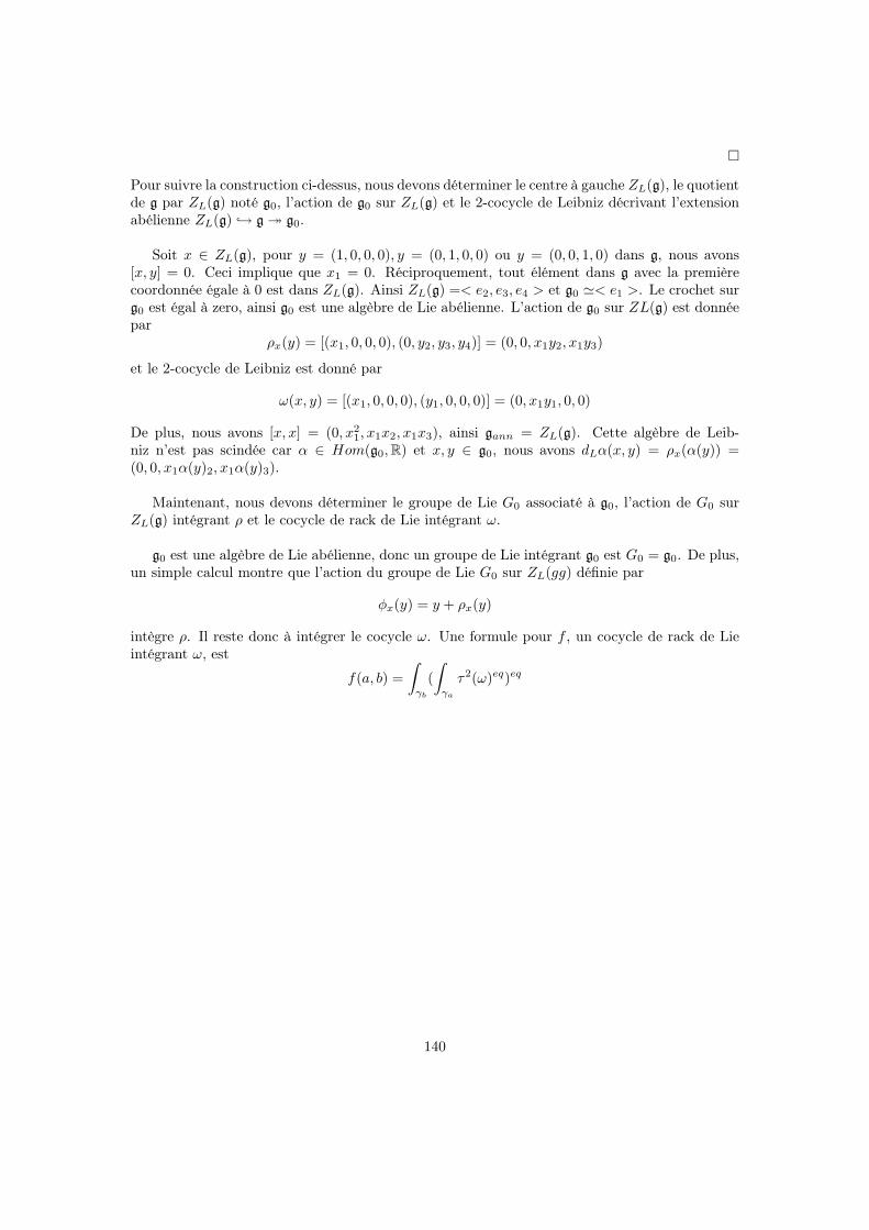
Pour suivre la construction ci-dessus, nous devons déterminer le centre à gauche ZL(g), le quotientde g par ZL(g) noté g0, l’action de g0 sur ZL(g) et le 2-cocycle de Leibniz décrivant l’extensionabélienne ZL(g) → g ։ g0.

Soit x ∈ ZL(g), pour y = (1, 0, 0, 0), y = (0, 1, 0, 0) ou y = (0, 0, 1, 0) dans g, nous avons[x, y] = 0. Ceci implique que x1 = 0. Réciproquement, tout élément dans g avec la premièrecoordonnée égale à 0 est dans ZL(g). Ainsi ZL(g) =< e2, e3, e4 > et g0 ≃< e1 >. Le crochet surg0 est égal à zero, ainsi g0 est une algèbre de Lie abélienne. L’action de g0 sur ZL(g) est donnéepar

ρx(y) = [(x1, 0, 0, 0), (0, y2, y3, y4)] = (0, 0, x1y2, x1y3)

et le 2-cocycle de Leibniz est donné par

ω(x, y) = [(x1, 0, 0, 0), (y1, 0, 0, 0)] = (0, x1y1, 0, 0)

De plus, nous avons [x, x] = (0, x21, x1x2, x1x3), ainsi gann = ZL(g). Cette algèbre de Leib-

niz n’est pas scindée car α ∈ Hom(g0,R) et x, y ∈ g0, nous avons dLα(x, y) = ρx(α(y)) =(0, 0, x1α(y)2, x1α(y)3).

Maintenant, nous devons déterminer le groupe de Lie G0 associaté à g0, l’action de G0 surZL(g) intégrant ρ et le cocycle de rack de Lie intégrant ω.

g0 est une algèbre de Lie abélienne, donc un groupe de Lie intégrant g0 est G0 = g0. De plus,un simple calcul montre que l’action du groupe de Lie G0 sur ZL(gg) définie par

φx(y) = y + ρx(y)

intègre ρ. Il reste donc à intégrer le cocycle ω. Une formule pour f , un cocycle de rack de Lieintégrant ω, est

f(a, b) =

∫

γb

(

∫

γa

τ2(ω)eq)eq

140

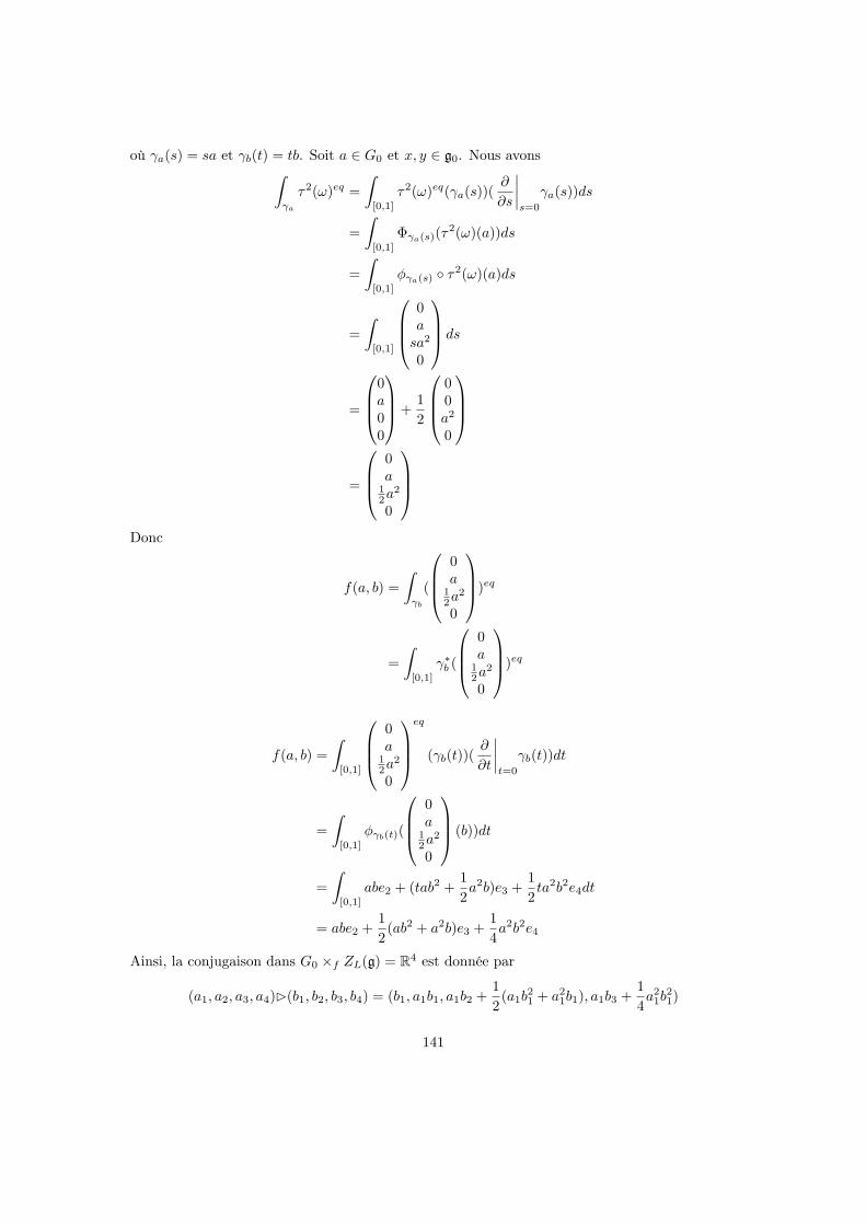
où γa(s) = sa et γb(t) = tb. Soit a ∈ G0 et x, y ∈ g0. Nous avons∫

γa

τ2(ω)eq =

∫

[0,1]

τ2(ω)eq(γa(s))(∂

∂s

∣∣∣∣s=0

γa(s))ds

=

∫

[0,1]

Φγa(s)(τ2(ω)(a))ds

=

∫

[0,1]

φγa(s) τ2(ω)(a)ds

=

∫

[0,1]

0asa2

0

ds

=

0a00

+

1

2

00a2

0

=

0a

12a

2

0

Donc

f(a, b) =

∫

γb

(

0a

12a

2

0

)eq

=

∫

[0,1]

γ∗b (

0a

12a

2

0

)eq

f(a, b) =

∫

[0,1]

0a

12a

2

0

eq

(γb(t))(∂

∂t

∣∣∣∣t=0

γb(t))dt

=

∫

[0,1]

φγb(t)(

0a

12a

2

0

(b))dt

=

∫

[0,1]

abe2 + (tab2 +1

2a2b)e3 +

1

2ta2b2e4dt

= abe2 +1

2(ab2 + a2b)e3 +

1

4a2b2e4

Ainsi, la conjugaison dans G0 ×f ZL(g) = R4 est donnée par

(a1, a2, a3, a4)⊲(b1, b2, b3, b4) = (b1, a1b1, a1b2 +1

2(a1b

21 + a2

1b1), a1b3 +1

4a21b

21)

141

Nous avons

∂2

∂s∂t |s,t=0(sa1, sa2, sa3, sa4)⊲(tb1, tb2, tb3, tb4) =

∂2

∂s∂t |s,t=0(tb1, sta1b1, sta1b2 +

1

2(st2a1b

21 + s2ta2

1b1),

sta1b3 + s2t21

4a21b

21)

= (0, a1b1, a1b2, a1b3)

= [(a1, a2, a3, a4), (b1, b2, b3, b4)]

Donc (R4,⊲) intègre (R4, [−,−]).

En dimension 5

Exemple B.3.34. Soit g = R5. Nous définissons une application bilinéaire sur g par

[e1, e1] = [e1, e2] = e3

[e2, e1] = [e2, e2] = [e1, e3] = e4

[e1, e4] = [e2, e3] = e5

et tous les crochets des autres combinaisons d’éléments de la base égaux à zéro. Nous avons

[(x1, x2, x3, x4), (y1, y2, y3, y4)] = (0, 0, x1(y1 + y2), x2(y1 + y2) + x1y3, x1y4 + x2y3)

Proposition B.3.35. (g, [−,−]) est une algèbre de Leibniz.

Preuve : Nous avons

[(x1, x2, x3, x4), [(y1, y2, y3, y4), (z1, z2, z3, z4)]] = (0, 0, 0, x1y1(z1+z2), x1(y2(z1+z2)+y1z3)+x2y1(z1+z2))

et

[(y1, y2, y3, y4), [(x1, x2, x3, x4), (z1, z2, z3, z4)]] = (0, 0, 0, x1y1(z1+z2), x1(y2(z1+z2)+y1z3)+x2y1(z1+z2))

et[[(x1, x2, x3, x4), (y1, y2, y3, y4)], (z1, z2, z3, z4)] = (0, 0, 0, 0)

Ainsi le crochet [−,−] satisfait l’identité de Leibniz.

Nous devons déterminer le centre à gauche ZL(g), le quotient de g par ZL(g) noté g0, l’actionde g0 sur ZL(g) et le 2-cocycle de Leibniz décrivant l’extension abélienne ZL(g) → g ։ g0.

Soit x ∈ ZL(g), pour y = (0, 0, 1, 0, 0) dans g, nous avons [x, y] = 0. Ceci implique quex1 = x2 = 0. Réciproquement, tout élément dans g avec les deux premières coordonnées égalesà 0 sont dans ZL(g). Ainsi ZL(g) =< e3, e4, e5 > et g0 ≃< e1, e2 >. Le crochet sur g0 est égal àzéro, ainsi g0 est une algèbre de Lie abélienne. L’action de g0 sur ZL(g) est donnée par

ρx(y) = [(x1, x2, 0, 0, 0), (0, 0, y3, y4, y5)] = (0, 0, 0, x1y3, x1y4 + x2y3)

et le 2-cocycle de Leibniz est donné par

ω(x, y) = [(x1, x2, 0, 0, 0), (y1, y2, 0, 0, 0)] = (0, 0, x1(y1 + y2), x2(y1 + y2), 0)

142

De plus, nous avons [x, x] = (0, 0, x1(x1 + x2), x2(x1 + x2) + x1x3, x1x4 + x2x3), ainsi enprenant x = (1, 0, 0, 0, 0), (0, 1, 0, 0, 0) and (0, 1, 1, 0, 0), on voit facilement que gann = ZL(g).Cette algèbre de Leibniz est non scindée car pour α ∈ Hom(g, ZL(g)) et x, y ∈ g0, nous avonsdLα(x, y) = ρx(α(y)) = (0, 0, 0x1α(y)3, x1α(y)4 + x2α(y)3).

Maintenant, nous devons déterminer le groupe de Lie G0 associé à g0, l’action de G0 surZL(g) intégrant ρ et le cocycle de rack de Lie intégrant ω.

L’algèbre de Lie g0 est abélienne, donc un groupe de Lie intégrant g0 est G0 = g0. Pourintégrer l’action ρ, nous utilisons l’exponentielle exp : End(ZL(g)) → Aut(ZL(g)). En effet, pourtout x ∈ g0, nous avons

ρx =

0 0 0x1 0 0x2 x1 0

ainsi, nous définissons un morphisme de groupe de Lie φ : G0 → Aut(ZL(g)) en posant

φx = exp(ρx) =

1 0 0x1 1 0

x2 + 12x

21 x1 0

Il est facile de voir que d1φ = ρ. Il reste donc à intégrer le cocycle ω. Une formule pour f , uncocycle de rack de Lie intégrant ω, est

f(a, b) =

∫

γb

(

∫

γa

τ2(ω)eq)eq

où γa(s) = sa et γb(t) = tb. Soit a ∈ G0 et x, y ∈ g0. Nous avons

∫

γa

τ2(ω)eq =

∫

[0,1]

τ2(ω)eq(γa(s))(∂

∂s

∣∣∣∣s=0

γa(s))ds

=

∫

[0,1]

Φγa(s)(τ2(ω)(a))ds

=

∫

[0,1]

φγa(s) τ2(ω)(a)ds

=

∫

[0,1]

1 0 0sa1 1 0

sa2 + 12 (sa1)

2 sa1 0

a1 a1

a2 a2

0 0

ds

=

∫

[0,1]

a1 a1

sa21 + a2 sa2

1 + a2

2sa1a2 + 12s

2a31 2sa1a2 + 1

2s2a3

1

ds

Donc∫

γa

τ2(ω)eq =

a1 a112a

21 + a2

12a

21 + a2

a1a2 + 16a

31 a1a2 + 1

6a31

143

Ainsi

f(a, b) =

∫

γb

(

∫

γa

τ2(ω)eq)eq

=

∫

γb

a1 a112a

21 + a2

12a

21 + a2

a1a2 + 16a

31 a1a2 + 1

6a31

eq

=

∫

[0,1]

γ∗b

a1 a112a

21 + a2

12a

21 + a2

a1a2 + 16a

31 a1a2 + 1

6a31

eq

=

∫

[0,1]

a1 a112a

21 + a2

12a

21 + a2

a1a2 + 16a

31 a1a2 + 1

6a31

eq

(γb(t))(∂

∂t

∣∣∣∣t=0

γb(t))dt

=

∫

[0,1]

φγb(t)(

a1 a112a

21 + a2

12a

21 + a2

a1a2 + 16a

31 a1a2 + 1

6a31

(b))dt

Nous avons

φγb(t)(

a1 a112a

21 + a2

12a

21 + a2

a1a2 + 16a

31 a1a2 + 1

6a31

(b)) =

1 0 0tb1 1 0

tb2 + 12 (tb1)

2 tb1 0

a1 a112a

21 + a2

12a

21 + a2

a1a2 + 16a

31 a1a2 + 1

6a31

(b1b2

)

=

a1(b1 + b2)(tb1a1 + a2 + 1

2a21)(b1 + b2)

(a1a2 + 16a

31 + 1

2 tb1a21 + tb2a1 + tb1a2 + 1

2 (tb1)2a1)(b1 + b2)

Donc

f(a, b) =

a1(b1 + b2)( 12b1a1 + a2 + 1

2a21)(b1 + b2)

(a1a2 + 16a

31 + 1

4b1a21 + 1

2b2a1 + 12b1a2 + 1

6 (b1)2a1)(b1 + b2)

et la conjugaison dans G0 ×f ZL(g) = R5 est donnée par

a1

a2

a3

a4

a5

⊲

b1b2b3b4b5

=

b1b2

b3 + a1(b1 + b2)a1b3 + b4 + ( 1

2b1a1 + a2 + 12a

21)(b1 + b2)

(a2 + 12a

21)b3 + a1b4 + b5 + (a1a2 + 1

6a31 + 1

4b1a21 + 1

2b2a1 + 12b1a2 + 1

6 (b1)2a1)(b1 + b2)

Avec un simple calcul, nous vérifions que

∂2

∂s∂t

∣∣∣∣s,t=0

(sa1, sa2, sa3, sa4, sa5)⊲(tb1, tb2, tb3, tb4, tb5) = [(a1, a2, a3, a4, a5), (b1, b2, b3, b4, b5)]

Donc (R5,⊲) intègre (R5, [−,−]).

144

Bibliography

[AG03] N. Andruskiewitsch and M. Graña. From racks to pointed hopf algebras. Adv. in Math.,178 (2):177–243, 2003.

[Bou72] N. Bourbaki. Groupes et algèbres de Lie-Parties 2 et 3. Hermann, 1972.

[Car30] E. Cartan. Le troisième théorème fondamental de Lie. C.R. Acad. Sc. t., 190:914, 1005,1930.

[CE56] H. Cartan and S. Eilenberg. Homological algebra. Princeton University Press, 1956.

[EG03] P. Etingof and M. Graña. On rack cohomology. Journal of pure and applied algebra,177:49–59, 2003.

[Est54] W.T. Van Est. A group theoretic interpretation of area in the elementary geometries.Simon Stevin, Wis. en Natuurkundig Tijdschrift, 32:29–38, 1954.

[Est62] W.T. Van Est. Local and global groups 1 and 2. Proc. Kon. Ned. Akad. v. Wet., SeriesA:391–425, 1962.

[Fel] R. Felipe. Generalized Loday algebra and digroups. preprint available athttp://www.cimat.mx/reportes/enlinea/I-04-01.pdf.

[FR] R. Fenn and C. Rourke. Racks and links in codimension two. available athttp://msp.warwick.ac.uk/ cpr/ftp/racks.ps.

[FRS95] R. Fenn, C. Rourke, and B. Sanderson. Trunks and classifying spaces. Applied categor-ical structures, 3:321–356, 1995.

[HS97] P.J. Hilton and U. Stammbach. A course in homological algebra. Springer-Verlag, 1997.Second edition.

[Jac] N. Jackson. Rack and quandle homology. available athttp://arxiv.org/pdf/math/0411055v1.

[Jac07] N. Jackson. Extensions of racks and quandles. Homology,Homotopy and applications,7 (1):151–167, 2007.

[Jub06] B. Jubin. Algebroids,cohomology and connections. 2006. Master’s thesis, unpublished.

[Kin07] M.K. Kinyon. Leibniz algebra, Lie racks and digroups. J.Lie Theory, 17:99–114, 2007.

[KW01] M.K. Kinyon and A. Weinstein. Leibniz algebras, Courant algebroïds, and multiplica-tions on reductive homogeneous spaces. American Journal of Mathematics, 123:525–550, 2001.

145

[Liu] K. Liu. A class of grouplike objects. available athttp://www.arXiv.org/math.RA/0311396.

[Lod93] J.-L. Loday. Une version non commutative des algèbres de Lie: les algèbres de Leibniz.L’Enseignement Mathématique, 39:269–293, 1993.

[Lod97] J.-L. Loday. Overview on Leibniz algebras, dialgebras and their homology. 17:91–102,1997. in Cyclic cohomology and noncommutative geometry.

[Lod98] J.-L. Loday. Cyclic Homology, volume 301. Springer, 1998. second edition.

[Lod01] J.-L. Loday. Dialgebras. Lecture Notes in Math., 1763:7–66, 2001. in Dialgebras andrelated operads.

[LP93] J.-L. Loday and T. Pirashvili. Universal envelopping algebras of Leibniz algebras and(co)homology. Math. Ann., 296:7–66, 1993.

[LP98] J.-L. Loday and T. Pirashvili. The tensor category of linear maps and Leibniz algebras.Georgian mathematical journal, 5(3):263–276, 1998.

[Mac95] S. Maclane. Homology, volume 114. Springer, 1995. second edition.

[Nee02] K.H. Neeb. Central extensions of infinite dimensional Lie groups. Ann. Inst. Fourier(Grenoble), 52 (5):1365–1442, 2002.

[Nee04] K.H. Neeb. Abelian extensions of infinite dimensional Lie groups. Travaux mathéma-tiques. Fasc. XV, Univ. Luxemb., pages 69–194, 2004.

[Pir94] T. Pirashvili. On Leibniz homology. Ann. Inst. Fourier (Grenoble), 44 (2):401–411,1994.

[Smi50] P.A. Smith. Some topological notions connected with a set of generators. ProceedingsInt. Cong., 2:436–441, 1950.

[Smi51] P.A. Smith. The complex of a group relative to a set of generators. Ann. of Math.,54:371–424, 1951.

146

147

Résumé : Le résultat principal de cette thèse est une solution locale du problème des coque-cigrues. Par problème des coquecigrues, nous parlons du problème d’intégration des algèbres deLeibniz. Cette question consiste à trouver une généralisation du troisième théorème de Lie pourles algèbres de Leibniz. Ce théorème établit que pour toute algèbre de Lie g, il existe un groupede Lie G dont l’espace tangent en 1 est muni d’une structure d’algèbre de Lie isomorphe à g. Lasructure d’algèbre de Leibniz généralise celle d’algèbre de Lie, nous cherchons donc une structurealgébrique généralisant celle de groupe et répondant à la même question. Nous résolvons ce prob-lème en intégrant localement toute algèbre de Leibniz en un rack de Lie augmenté local. Un rackde Lie étant une variété munie d’un produit satisfaisant plusieurs axiomes qui généralisent despropriétés de la conjugaison dans un groupe. En particulier, ce produit est autodistributif. Notreapproche de ce problème est basée sur une preuve donnée par E.Cartan dans le cas des groupes etalgèbres de Lie, et consiste à associer à toute algèbres de Leibniz une extension abélienne d’unealgèbre de Lie par un module antisymétrique. Cette extension est caractérisée par une classedans le second groupe de cohomologie de Leibniz, et nous associons à tous représentant de cetteclasse un cocyle de rack de Lie local qui nous permet de construire un rack de Lie augmenté localrépondant au problème. Pour construire ce cocycle, nous généralisons une méthode d’intégrationd’un cocycle d’algèbre de Lie en cocycle de groupe de Lie due à W.T.Van Est.

Summary : The main result of this thesis is a local answer to the coquecigrue problem.By coquecigrue problem, we mean the problem of integrating Leibniz algebras. This questionconsists in finding a generalization of Lie’s third theorem for Leibniz algebras. This theoremestablishes that for every Lie algebra g, there exists a Lie group G whose tangent space at 1is provided with the structure of a Lie algebra isomorphic to g. The Leibniz algebra structuregeneralizes that of a Lie algebra, so we search for an algebraic structure generalizing that of agroup and answering the same question. We answer to this problem by locally integrating everyLeibniz algebra into a local augmented Lie racks. A Lie rack being a manifold provided witha product satisfying further axioms which generalize (some properties of) the conjugation in agroup. Particularly we ask this product to be self distributive. Our approach to the problemis similar to one given by E. Cartan in the case of Lie groups and Lie algebras, and consists inassociating to every Leibniz algebra an abelian extension of a Lie algebra by an anti-symmetricmodule. This extension is caracterised by a class in the second Leibniz cohomology group, andwe associate to a representant of this class a local Lie rack cocycle which permits us to construct alocal augmented Lie rack which solves the problem. To construct this local cocycle, we generalizean integration method of a Lie algebra cocycle into a Lie group cocycle due to W.T. Van Est.

Mots clés : algèbre de Leibniz, coquecigrue, rack de Lie, cohomologie d’algèbre de Leibniz,cohomologie de rack, intégration des cocycles de Leibniz.

Discipline : Mathématiques

N :