The University of Manchester Research

Linking Continuous and Recycle Emulsication Kinetics forIn-line mixers.DOI:10.1016/j.cherd.2018.02.003

Document VersionAccepted author manuscript

Link to publication record in Manchester Research Explorer

Citation for published version (APA):Carrillo De Hert, S., & Rodgers, T. (2018). Linking Continuous and Recycle Emulsication Kinetics for In-line mixers.Chemical Engineering Research & Design, 132, 922-929. https://doi.org/10.1016/j.cherd.2018.02.003

Published in:Chemical Engineering Research & Design

Citing this paperPlease note that where the full-text provided on Manchester Research Explorer is the Author Accepted Manuscriptor Proof version this may differ from the final Published version. If citing, it is advised that you check and use thepublisher's definitive version.

General rightsCopyright and moral rights for the publications made accessible in the Research Explorer are retained by theauthors and/or other copyright owners and it is a condition of accessing publications that users recognise andabide by the legal requirements associated with these rights.

Takedown policyIf you believe that this document breaches copyright please refer to the University of Manchester’s TakedownProcedures [http://man.ac.uk/04Y6Bo] or contact uml.scholarlycommunications@manchester.ac.uk providingrelevant details, so we can investigate your claim.

Download date:27. Jun. 2019

Linking Continuous and Recycle Emulsification Kinetics

for In-line mixers.

Sergio Carrillo De Hert, Thomas L. Rodgers∗

School of Chemical Engineering and Analytical Science, The University of Manchester,Manchester M13 9PL, U.K.

Abstract

In-line high-shear mixers can be used for continuous or batch dispersion operations depend-ing on how the pipework is arranged. In our previous work (Carrillo De Hert and Rodgers,2017a) we performed a transient mass balance to establish the link in-between these twoarrangements; however this model was limited to the estimation of the mode of dispersedphases yielding simple monomodal drop size distributions. In this investigation we expandedthe previous model to account for the shape of the whole drop size distribution. The newmodel was tested by performing experiments under different processing conditions andusing two highly viscous dispersed phases which yield bimodal drop size distributions. Theresults for the continuous arrangement experiments were fit using two log-normal functionsand the results for the recycle arrangement by implementing the log-normal function in thepreviously published mass balance. The new model was capable of predicting the d32 fordifferent emulsification times with a mean absolute error of 12.32%. The model presentedhere was developed for liquid blends, however the same approach could be used for millingor de-agglomeration operations.

Keywords: Emulsification, In-line rotor-stator, In-line high-shear mixer,

Continuous emulsification, Batch emulsification, Bimodal Drop Size

Distribution

∗Corresponding author: +44 (0)161 306 8849Email addresses: sergio.carrillodehert@manchester.ac.uk (Sergio Carrillo De

Hert), tom.rodgers@manchester.ac.uk (Thomas L. Rodgers )

Preprint submitted to Chemical Engineering Research and Design January 28, 2018

Nomenclature

Latin symbolsQ flow rate [m3 s−1]dG logarithmic mean of the log-

normal distribution [m]dG,n,x logarithmic mean of the log-

normal distribution for the nthpass for:x = L large and x = ssmall drops[m]

tres,T mean residence time in the tank[s]

Ai ith fit constant [-]Bi ith fit constant [-]di diameter of the ith drop class

[meter]fv,n,x(di) frequency of the ith drop size af-

ter n passes for x = L large, x = ssmall or x = T total distribution[-]

fv,Rec(di) frequency of the ith drop sizefor the recycle arrangement [-]

Fv(di) cumulative distribution of the ithdrop size [-]

Mon mode of the distribution for npasses [m]

Mon,x mode of the distribution after npasses for: x = L large or x = ssmall drops [m]

MoRec mode of the distribution in therecycle arrangement [m]

N stirring speed [s−1]n number of passes [-]R2 coefficient of determination [-]sG logarithmic standard deviation of

the log-normal distribution [m]t time [s]VT volume of the vessel [meter3]

Greek symbolsµd viscosity of the dispersed phase

[Pa s]φn volume fraction of the material for

n-passes [-]φs,n relative volume fraction of the

small drops after n-passes [-]

Dimensionless numbersPo Power number PN−3D−5ρ−1

AbbreviationsDSD Drop size distributionRS Rotor-statorSiOil Silicon Oil

Introduction1

In-line rotor-stators (RS) are one of the most promising equipments that2

have been implemented to intensify dispersion processes. Their increase in3

popularity has been due to their capacity to generate highly-localised strong4

energy dissipation regions. In-line RS are installed in the pipework and5

two different types of operation arrangements are possible depending on the6

direction of the outflow of the RS. (1) If the outflow is directed to a secondary7

vessel or process, the RS is operated in a continuous fashion; evidently the8

2

material can be processed n number of times to cause further size reduction,9

“multi-pass processing” occurs when the material is processed n > 1 times. (2)10

On the other hand, if the outflow is directed to the feeding tank it is operated11

in a recycle arrangement and processing time and volume becomes important12

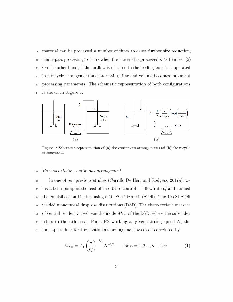
processing parameters. The schematic representation of both configurations13

is shown in Figure 1.14

(a) (b)

Figure 1: Schematic representation of (a) the continuous arrangement and (b) the recyclearrangement.

Previous study: continuous arrangement15

In one of our previous studies (Carrillo De Hert and Rodgers, 2017a), we16

installed a pump at the feed of the RS to control the flow rate Q and studied17

the emulsification kinetics using a 10 cSt silicon oil (SiOil). The 10 cSt SiOil18

yielded monomodal drop size distributions (DSD). The characteristic measure19

of central tendency used was the mode Mon of the DSD, where the sub-index20

refers to the nth pass. For a RS working at given stirring speed N , the21

multi-pass data for the continuous arrangement was well correlated by22

Mon = A1

(n

Q

)−1/5

N−6/5 for n = 1, 2, .., n− 1, n (1)

3

where (n/Q) is proportional to the residence time of the material inside the23

RS. We attribute the effect of mean residence time to the internal recirculation24

or fluid re-entrainment inside the RS, this has been reported by authors such25

as Ozcan-Taskin et al. (2011) and Mortensen et al. (2017) using particle26

image velocimetry and by Xu et al. (2014) using laser Doppler anemometry.27

Therefore the lower Q the more times the emulsions re-enters the region where28

drop breakup occurs.29

We did not do experiments at different scales, however there is strong30

evidence that the characteristic volume of the RS is its swept volume (Hall31

et al., 2013). Hall et al. (2011) did not find a correlation in-between the32

coarse emulsion (n = 0) and the one at the outlet of the RS, therefore in33

the continuous arrangement all the information of the coarse emulsion is lost34

after one pass is completed.35

In a second study (Carrillo De Hert and Rodgers, 2017b), we extended

Equation 1 to account for the effect of the viscosity of the dispersed phase µd

by doing experiments using SiOils in the 10 cSt-30 000 cSt range. We found

that SiOils thicker the 350 produced bimodal DSD. The mode of the large

Mon,L and the mode of the small Mon,s drops were used to characterise the

drop sizes of the emulsion, for the same geometry used in (Carrillo De Hert

and Rodgers, 2017a) the following correlations were obtained for the SiOil in

the 10 cSt-2760 cSt range

Mon,L =1.18× 105µ0.365d N−1.05

(n

Q

)−1/5

(2)

Mon,s =1.69× 103µ−0.365d N−1.05 (3)

4

Furthermore we correlated the DSDs using a simple mixing rule36

fv,n,T (di) = (1− φs,n) fv,n,L(di) + φs,nfv,n,s(di) (4)

where fv,n,T (di) is the total drop size distribution; fv,n,L(di) and fv,n,s(di) are37

the drop size distribution of the large and small drops respectively; and φs,n38

is the volume fraction of the small drops for the nth pass through the RS. We39

further used Generalised Gamma probability density functions for fv,n,L(di)40

and fv,n,s(di) and the power-law function below for φs,n41

φs,n = Cφ,0µCφ,µdd NCφ,N

(n

Q

)Cφ,t(5)

Previous study: recycle arrangement42

In the recycle arrangement (see Fig. 1b) a coarse emulsion (t = 0) is43

pumped through the RS and back into the its feeding vessel. For t > 0 it is44

expected to have a mixture of material that has passed n times, the fraction45

of each material φn is a function of time t, volume of the vessel VT and of Q.46

As can be expected, the DSD distribution of the coarse emulsion is important47

in this arrangement until its complete consumption.48

In Carrillo De Hert and Rodgers (2017a) we did a transient mass balance49

to obtain φn as a function of the aforementioned variables, the expression for50

φn reads51

φn =1

n!

(t

tres,T

)nexp

(− t

tres,T

)(6)

where tres,T = VT/Q is the mean residence time of the material in the tank.52

Equation 6 was tested by (1) measuring the depletion of the coarse emulsion as53

5

a function time, as the n = 0 and n > 0 materials produced two very distinct54

peaks and by (2) predicting the mode of the distribution of the mixture of the55

n > 0 drops MoRec. Provided that the continuous arrangement experiments56

showed that the DSD for n > 0 were monomodal and had the same shape, a57

mixing rule to estimate the Mo was used58

MoRec =∑n=1

φn1− φ0

Mon (7)

Substituting Equation 1 and 6 in Equation 7 lead to59

MoRec =A1Q

1/5

N 6/5

[exp

(t

tres,T

)− 1

]∑n=1

1

n1/5n!

(t

tres,T

)n(8)

Equations 8 is limited to monomodal distributions and to the calculation of the60

mode, in this study we will expand our two previous studies (Carrillo De Hert61

and Rodgers, 2017a,b) to systems yielding bimodal drop size distributions,62

which are common for highly viscous dispersed phases.63

Materials and equipment and methods64

Materials65

Two 200 Silicone Fluid (dimethyl siloxane, Dow Corning, Michigan, USA)66

of 350 cSt and 1000 cSt nominal kinematic viscosity were used as dispersed67

phases. Their relevant properties are listed in Table 1. The specific gravity s68

was taken as given by the provider and the µd were obtained using a DV2T69

Viscometer (Brookfield Viscometers, Essex, UK).70

As continuous phase 1 wt.% of sodium laureth sulfate (SLES) in water was71

6

used; SLES is the surfactant, in Texapon N701 (Cognis, Hertfordshire, UK)72

at 70wt.%. The surfactant concentration was approximately 120 times the73

critical micellar concentration found by El-Hamouz (2007) for Texapon N701.74

The interfacial tension in-between the dispersed phases and the continuous75

phase σ are also shown in Table 1; these were obtained using a K11 Mk476

Tensiometer (KRUSS, Hamburg, Germany) and a KRUSS platinum-iridium77

standard ring.78

Table 1: Relevant properties of the Silicon Oils used at 25 ◦C. These same properties havebeen previously reported in Carrillo De Hert and Rodgers (2017a,b)

SiOil [cSt] s [-] µd [Pa s] σ [N m]350 0.965 3.279× 10−1 9.129× 10−3

1000 0.970 9.474× 10−1 9.172× 10−3

Equipment79

The same L5M-A Laboratory Mixer (Silverson Machines, Chesham, UK),80

rotor, screen and peristaltic pump in Carrillo De Hert and Rodgers (2017a,b)81

were used for this study. The characteristics of the rotor and the screen are82

listed in Table 2.83

Table 2: Geometrical characteristics of the rRS.

Rotor ScreenDiameter 3.0 cm Inner diameter 3.2 cmNumber of blades 4 Outer diameter 3.4 cmHeight 1.0 cm Stator height 2.0 cmBlade thickness 0.5 cm Hole arrangement 6x40, pitchedMaximum speed (nominal) 133 s−1 Number of holes 240

7

Methods84

The coarse emulsions were prepared using an unbaffled cylindrical vessel85

with diameter of 25 cm and a 8-blade Rushton turbine with a diameter of86

6.62 cm. After dissolving the SLES completely (1.0wt%), the stirring speed87

was fixed to the desired stirring speed and the SiOil was poured (1v.%). The88

systems were stirred for 24 h to ensure that all drop break-up was due to the89

RS and not to the impeller in the vessel.90

For the continuous arrangement, the coarse emulsion was fed to the RS at91

the experimental conditions specified in Table 3. After the volume in feeding92

tank was consumed, the connecting tubes were rinsed with fresh water and93

purged. The tanks were swapped and the process was repeated for n number94

of passes. Samples were taken after the whole volume was processed while95

the tank was being stirred.96

The recycle arrangement experiments were performed at the same Q and97

N as for the continuous arrangements under the conditions specified in Table98

3. Samples were taken for different t.99

Table 3: Experimental conditions of experiments performed. The number inside parenthesisindicate the number of samples taken at different times.

350 cSt 1000 cStArrangements-Shared

Q [m3 s−1] 2.90× 10−5 9.08× 10−9

Impeller N [s−1] 11.9 11.7RS N [s−1] 50.00 166.7

Continuousn [-] 0-7 0-7

RecycleVT [m3] 13× 10−3 10× 10−3

t [s] 0-4544 (8) 0-10 000 (8)

8

Sampling was done approximately 5 cm below the liquid level. The samples100

were stored and analysed as soon as the previous sample was analysed.101

The experimental conditions listed in Table 3 were chosen to provide an102

example where the DSD for n = 0 and for n > 0 were close (350 cSt) and an103

example where these were more separated (1000 cSt) within the experimental104

range where the correlations obtained in Carrillo De Hert and Rodgers (2017b)105

have been proven.106

The DSDs were analysed using the Mastersizer 3000 (Malvern Instruments,107

Malvern, UK). The complex refractive index used was 1.399 + 0.001i and108

the details of the Standard Operation Procedure used has been previously109

detailed in Carrillo De Hert and Rodgers (2017a) and Carrillo De Hert and110

Rodgers (2017b).111

Log-normal fits for previous work in Carrillo De Hert and Rodgers112

(2017b)113

The data exported by the Mastersizer 3000 is presented as a cumulative114

frequency histogram where∑fv(di) = 100. In our previous work (Carrillo De115

Hert and Rodgers, 2017b) we normalized the DSD exported from the Master-116

sizer by making the area under the curve equal 100%, this was done in order117

to transform the cumulative frequency histogram into a probability density118

distribution. After normalizing, the DSD were fit using probability density119

functions. However, the integration and normalisation of the experimental120

data is not required if the difference between the cumulative frequency of the121

ith drop diameter Fv(di) and the one of the (i− 1)th drop diameter Fv(di−1)122

9

is used123

fv(di) = Fv(di)− Fv(di−1) (9)

The DSD were fit using a mixing rule (Eq. 4) and we used two Generalised124

Gamma functions (GGf) to fit our results in Carrillo De Hert and Rodgers125

(2017b). The GGf has three parameters: one that controls its scale, another126

that controls its broadness and a third one that affects the symmetry (low127

values yield skewed distributions, the opposite is true for large values) of the128

distribution. A large value for the latter was chosen and was kept constant129

for all our fits.130

In this investigation it was shown that log-normal distributions are also131

adequate to describe the shape of the DSD and also give a good estimation132

of the d32. The equation of the cumulative function reads133

Fv(di) =1

2+

1

2erf

(ln di − dG√

2sG

)(10)

where dG is the logarithmic mean of the DSD and sG the logarithmic standard134

deviation.135

In this section we provide the new fit parameters for the simplified fit-136

scheme based on two log-normal cumulative distributions. The fit to the DSD137

was performed using a power-law function for dG (Eq. 11 below), the indexes138

are known from the analysis of variance (ANOVA) done for the modes in139

Carrillo De Hert and Rodgers (2017b) and the only parameter for dG,L and140

dG,s obtained using the method of the least squares were the pre-exponentials141

10

CG,L and CG,s142

dG = ln

[CGµ

CG,µd NCG,N

(n

Q

)CG,t](11)

The standard deviations of the distributions (sG,L and sG,s) were also obtained143

using the method of the least squares but these were considered to be indepen-144

dent of µ and the processing conditions. The coefficient obtained using the145

least square method for Equation 11 and the standard deviations are listed in146

Table 4. If this table is compared with Equation 2 and Equation 3 it can be147

seen that the value of CG,N was changed from -1.05 to -1.2. The former value148

was obtained directly from the ANOVA in Carrillo De Hert and Rodgers149

(2017b); however changing its value to -1.2 produces no significant variation150

in the goodness of the fit (within our experimental range 50-166.67 s−1) while151

being in agreement with the well-know theory developed by Hinze (1955).152

Table 4: Constants obtained for the log-normal distributions for the large and small typeof drops for Eqs. 11 and 10.

Parameter Large SmallCG 2.10× 105 3.40× 103

CG,µ 0.365 -0.365CG,N -1.2 -1.2CG,t -0.2 0sG 0.400 0.843

Simultaneously the φs for each distribution were “freely fit”. As recognized153

in our previous work (Carrillo De Hert and Rodgers, 2017b), this is the most154

difficult parameter to obtain a correlation for. The power-law function shown155

11

below was also used to correlated the data156

φs = CφµCφ,µd NCφ,N

(n

Q

)Cφ,t(12)

The ANOVA for Equation 12 yielded Cφ,µ = 0.025 ± 85.2% and a p-value157

of 0.0223, therefore the effect of µd was considered negligible due to its low158

statistical significance. Under these considerations, the ANOVA yielded the159

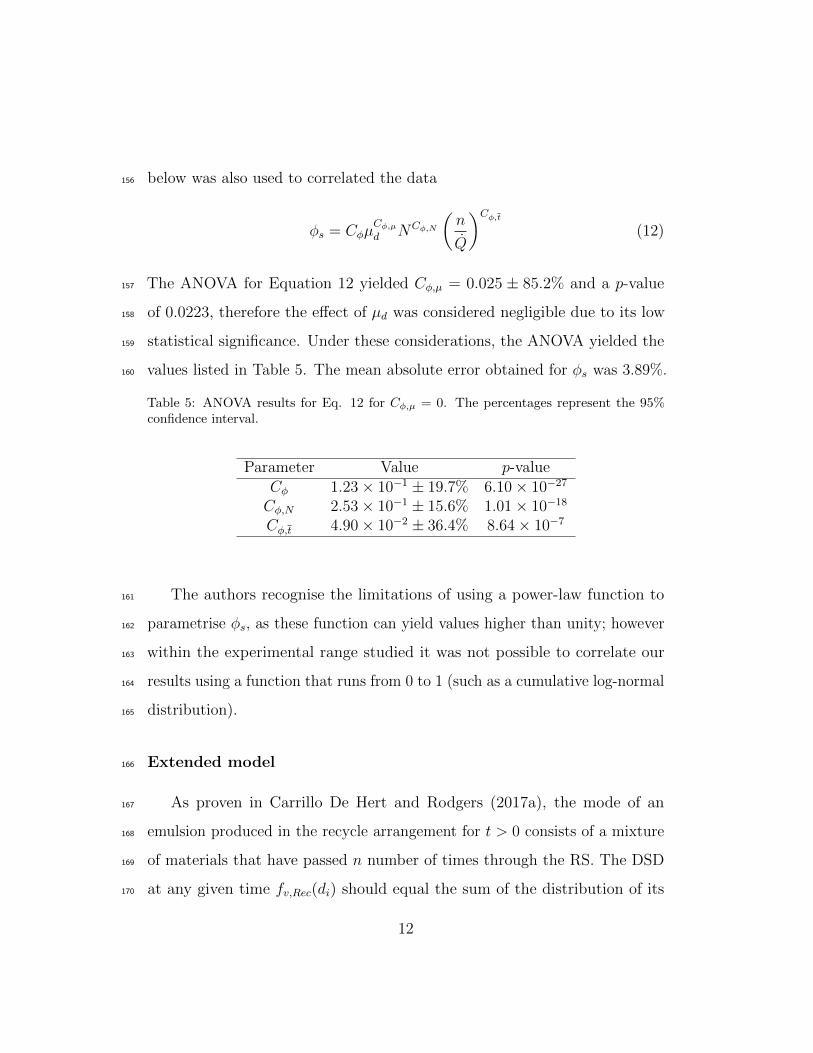
values listed in Table 5. The mean absolute error obtained for φs was 3.89%.160

Table 5: ANOVA results for Eq. 12 for Cφ,µ = 0. The percentages represent the 95%confidence interval.

Parameter Value p-valueCφ 1.23× 10−1 ± 19.7% 6.10× 10−27

Cφ,N 2.53× 10−1 ± 15.6% 1.01× 10−18

Cφ,t 4.90× 10−2 ± 36.4% 8.64× 10−7

The authors recognise the limitations of using a power-law function to161

parametrise φs, as these function can yield values higher than unity; however162

within the experimental range studied it was not possible to correlate our163

results using a function that runs from 0 to 1 (such as a cumulative log-normal164

distribution).165

Extended model166

As proven in Carrillo De Hert and Rodgers (2017a), the mode of an167

emulsion produced in the recycle arrangement for t > 0 consists of a mixture168

of materials that have passed n number of times through the RS. The DSD169

at any given time fv,Rec(di) should equal the sum of the distribution of its170

12

composing materials171

fv,Rec(di) =∑n=0

φnfv,n(di) (13)

where φn can be obtained by Equation 6 and fv,n(di) is the frequency of the172

ith drop size for the material that has passed n number of times through the173

RS.174

The examples that will be given in Section 5 consist of bimodal coarse

emulsions and bimodal DSD for any n > 0. Using the mixing rule in Equation

4, the following equation can be derived

fv,Rec(di) =φ0fv,0(di) +∑n=1

φnfv,n(di)

=φ0 [(1− φs,0) fv,0,L(di) + φs,0fv,0,s(di)] +∑n=1

φn [(1− φs,n) fv,n,L(di) + φs,nfv,n,s(di)] (14)

where φs,n is the relative volume fraction of the small drops of the material

that has passed n-times through the RS and, fv,n,L(di) and fv,n,s(di) are the

frequency of the ith drop size of the material for n-passes for the large and

small types of drops respectively. Substituting Equation 6 in 14 yields

fv,Rec(di) = exp

(− t

tres,T

){[(1− φs,0) fv,0,L(di) + φs,0fv,0,s(di)] +∑

n=1

1

n!

(t

tres,T

)n[(1− φs,n) fv,n,L(di) + φs,nfv,n,s(di)]

}(15)

As seen in Section 5, fv,n,L(di) and fv,n,s(di) can be given by cumulative175

log-normal distribution difference and φs,n by a power-law function.176

13

Results and discussion177

Continuous arrangement results178

The results obtained for both SiOil are shown in Figure 2. The same179

trends found in Carrillo De Hert and Rodgers (2017b) were observed: (1) no180

steady-state DSD was found for n = 7 and (2) the large drops are n-dependent181

while the small drops are n-independent (see Fig. 3).182

100 101 102 1030

2

4

6

8

10

12

f v(di ) [

%]

di [ m]

n [-] 0 4 1 5 2 6 3 7

(a)

100 101 102 1030

2

4

6

8

10

f v(di ) [

%]

di [ m]

n [-] 0 4 1 5 2 6 3 7

(b)

Figure 2: DSD obtained for n = 1, 2, ..., 7 passes in the continuous arrangement for the (a)350 cSt SiOil and (b) 1000 cSt SiOil.

1 2 3 4 5 6 7 82x100

2x101

2x102

101

102

MoL= 52.5n-0.2

MoL= 138n-0.2

350 cSt MoL

1000 cSt MoL Mos

Mo L ,

Mo s [

m]

n [-]

Mos= 6.71 m

Figure 3: Modes of the DSDs shown in Fig. 2 as a function of n for both SiOils.

14

The DSD were fit using the cumulative log-normal distributions. Never-183

theless, the parametrization was only done as a function of n for each set of184

experiments to prove the extended model (Sec. 4) in Section 5.2 with the185

most accurate accurate parameters.186

The fit for the coarse material was fit independently of the n > 0 distribu-187

tions, as no correlation in-between these was found in this work nor by Hall188

et al. (2011). The logarithmic mean of the large drops of the coarse emulsion189

dG,0,L, their logarithmic standard deviation sG,0,L along with these parameter190

for the small drops dG,0,s and sG,0,s and their volume fraction φs,0 are listed191

in Table 6 for the coarse emulsions obtained for both SiOils.192

For the n > 0 distributions, the large drop sizes are n-dependent and, as193

shown in Figure 3 and in Carrillo De Hert and Rodgers (2017b), these are194

well-correlated by n−0.2, the following model was proposed for the logarithmic195

mean of the large drops196

dG,n,L = ln(B1n

−1/5)

(16)

The rest of the parameters of the log-normal cumulative distribution for the197

large and small drops were considered constant and were not parametrised,198

however φs,n was, because it is n-dependent (Carrillo De Hert and Rodgers,199

2017b)200

φs,n>0 = B2nB3 (17)

The values of all the variables for the large and small drops for n > 0 are also201

displayed in Table 6, while two examples of the appearance of the fits are202

shown in Figure 4.203

15

100 101 102 1030

2

4

6

8 Experimental (1- s,4 )fv,4,L(di)

s,4 fv,4,s(di) fv,4(di)

f v(d i

) [%

]

di [ m]

(a)

100 101 102 1030

2

4

6

Experimental (1- s,2 )fv,2,L(di)

s,2 fv,2,s(di) fv,2(di)

f v(d i

) [%

]

di [ m]

(b)

Figure 4: Examples of fits: (a) 350 cSt SiOil for n = 4 and (b) 1000 cSt SiOil for n = 2.

Table 6: Fit parameters for the dual log-normal cumulative distribution fit for the 350 cStand 1000 cSt SiOils.

Parameter 350 cSt 1000 cSt

dG,0,L 5.69 6.51sG,0,L 0.432 0.443

dG,0,s 4.43 5.53sG,0,s 0.650 0.855φs,0 0.878 0.595B1 139 56.6

sG,n>0,L 0.44 0.45

dG,n>0,s 3.59 1.90sG,n>1,s 0.861 0.792

B2 0.628 0.234B3 -0.0688 -0.111

Recycle arrangement results204

Figure 5 shows the DSDs obtained using the recycle arrangement for the205

same Q and N used for the continuous arrangement for different processing206

times. Figure 5a provides an example where the DSD decreases progressively207

16

and the consumption of the coarse emulsion cannot be tracked directly. As208

will be shown later, the progressive size reduction is due to the close proximity209

in-between the DSDs obtained for n = 0 and the n > 0 (see Fig. 2a). In210

Figure 5b the consumption of the coarse emulsion is more evident because211

the DSDs of the coarse emulsion and the material that has passed through212

the rotor-stator are further apart.213

100 101 102 1030

2

4

6

8

10

12

f v(di ) [

%]

di [ m]

t [s] 0 47 129 229 358 539 850 2064 4544 10000

(a)

100 101 102 1030

2

4

6

8

10

f v(di ) [

%]

di [ m]

t [s] 0 100 2154 215 3154 464 4800 1000 10 000

(b)

Figure 5: DSDs for the recycle arrangement for different times for the conditions listed inTable 3 for (a) the 350 cSt SiOil and for (b) the 1000 cSt SiOil.

Equation 15 was combined with Equations 9, 10 and with the fit constants214

obtained for the continuous arrangement experiments listed in Table 6 to fit215

the recycle arrangement DSDs shown in Figure 5.216

Examples of the fit are shown in Figure 6. Figure 6a shows an example of217

the composition of each of the drop size distributions for t > 0. As can be218

seen in this figure, the coarse emulsion has not been completely consumed219

and the contribution of the materials that has passed n = 1, 2, 3 are the main220

responsible for the change in the shape of the DSD. On the other hand, Figure221

6b shows the total fit for three different times, it can be seen that the model222

17

is accurate in predicting even very complex DSD.223

100 101 102 1030

2

4

6

8

f v(di ) [

%]

di [ m]

Experimental 0 fv,0 (di )

1 fv,1 (di )

2 fv,2 (di )

3 fv,3 (di )

n=4 n fv,n (di )

n=0 n fv,n (di )

(a)

100 101 102 1030

2

4

6

8

10 t [s] Exp. Fit 0 464 10 000

f v(di ) [

%]

di [ m]

(b)

Figure 6: Examples of the fit using the new model. (a) Shows the contribution of thedifferent materials for the DSD obtained for t = 358 s for the 350 cSt SiOil; (b) shows thetotal fit for the 1000 cSt SiOil experiment for three different times.

The goodness of the fit was assessed by comparing the experimental and224

predicted d32. The obtained coefficient of determination R2 obtained were225

0.997 and 0.980 for the 350 cSt and 1000 cSt SiOils respectively, while the226

mean absolute error were 12.32% and 9.51%. The experimental and predicted227

d32 as a function of time in log-log scale are shown in Figure 7, where it can228

be seen that the models follow the complex trend reasonably well.229

Conclusions and recommendations for future work230

The transient mass balance derived in our previous work Carrillo De231

Hert and Rodgers (2017a) can be used to predict the evolution of the DSD232

with time by using the mixing rule in Equation 14. The mixing rule could233

be implemented to bimodal DSD. As shown in the examples presented,234

future study of multiphase systems in RSs has to be done preferably (if not235

18

101 102 103 1045

20

50

200

10

100

d 32 [

m]

t [s]

Experimental 350 cSt 1000 cSt

Fit 350 cSt 1000 cSt

Figure 7: Experimental and predicted d32 as a function of time for both SiOils.

exclusively) using the continuous arrangement to remove misleading mass236

balance features. The authors consider that the models presented in Carrillo237

De Hert and Rodgers (2017a) and in this investigation provide a strong238

fundamental basis to extrapolate continuous arrangement results to recycle239

systems, provided that the vessel is well-mixed.240

There have been multiple studies (Badyga et al. (2008); Padron et al.241

(2008); Ozcan-Taskin et al. (2009, 2016) among others), which have used the242

recycle arrangement to study the de-agglomeration of nano-particles. These243

authors have explained breakup in terms of shattering, rupture or erosion244

mechanisms. Figure 5a resembles the rupture mechanism for nanoparticles245

while Figure 5b resembles the shattering one. However, we have shown that246

the trends in these figures are due to mass balance features and by the247

proximity in-between the DSD of the coarse and processed materials. Future248

work on breakup mechanism require the separation of the break-up inside the249

rotor stator and mass balance effects. Ideally experiments with the continuous250

arrangement should be used.251

The semi-empirical model for emulsification in the continuous arrangement252

19

presented here and in our previous work (Carrillo De Hert and Rodgers,253

2017a,b) (Eqs. 1, 2 and 3) consider that the drop sizes are proportional to the254

mean residence time inside the RS which is further proportional to(n/Q

)−1/5

;255

this can be explained by the internal recycling inside the RS (reported by256

Ozcan-Taskin et al. (2011); Mortensen et al. (2017); Xu et al. (2014) among257

others). However it is unknown if the −1/5 index is universal or depends on258

the geometrical characteristics of the RSs. Hall et al. (2013) reported indexes259

of -0.148 and -0.043 for 10 cSt and 350 cSt SiOils respectively, but their260

results were correlated to the d32 and their emulsions were produced using a261

double-rotor-double-stator geometry. The lower residence time dependency262

reported by Hall et al. (2013) for the thickest oil is most likely due to the263

small daughter drops which make the d32 trend smoother because these are264

mean residence time-independent. To our knowledge there is no other work265

in literature which uses the mode or the maximum drop diameter to know266

the mean residence time dependency.267

The drop size dependency with N has more theoretical basis as its index268

is in agreement with the mechanistic models developed by Hinze (1955) and269

Shinnar and Church (1960) even though these were postulated for steady-state270

systems. Finally the study on the µd dependency in (Carrillo De Hert and271

Rodgers, 2017b) (Eqs. 2 and 3) is unique as most of the correlations found272

in literature use the d32 and do not track the individual drop size change273

nor the relative volume fraction of each type of drop produced which makes274

comparison with other work in literature virtually impossible. Future work275

should also focus on analysing the whole DSDs and not only the d32, specially276

for highly-viscous dispersed phases which tend to produce bimodal DSD.277

20

Funding and Acknowledgements278

The authors would like to express their gratitude to the Mexican Na-279

tional Council for Science and Technology (CONACYT) for supporting this280

project as part of the first author’s PhD studies through the CONACYT-The281

University of Manchester fellowship program.282

The authors would also like to thank the workshop staff of The University283

of Manchester’s School of Chemical Engineering and Analytical Science for284

their help with the modifications and maintenance of the equipment.285

Bibliography286

Badyga, J., Makowski, L., Orciuch, W., Sauter, C., Schuchmann, H. P., 2008.287

Deagglomeration processes in high-shear devices. Chemical Engineering288

Research and Design 86 (12), 1369 – 1381, international Symposium on289

Mixing in Industrial Processes (ISMIP-VI).290

URL http://www.sciencedirect.com/science/article/pii/S0263876208002542291

Carrillo De Hert, S., Rodgers, T. L., 2017a. Continuous, recycle and batch292

emulsification kinetics using a high-shear mixer. Chemical Engineering293

Science 167, 265–277.294

Carrillo De Hert, S., Rodgers, T. L., 2017b. On the effect of dispersed phase295

viscosity and mean residence time on the droplet size distribution for high-296

shear mixers. Chemical Engineering Science 172 (Supplement C), 423 – 433.297

URL http://www.sciencedirect.com/science/article/pii/S0009250917304426298

El-Hamouz, A., may 2007. Effect of surfactant concentration and operating299

21

temperature on the drop size distribution of silicon oil water dispersion.300

Journal of Dispersion Science and Technology 28 (5), 797–804.301

Hall, S., Cooke, M., El-Hamouz, A., Kowalski, A., may 2011. Droplet break-302

up by in-line silverson rotor-stator mixer. Chemical Engineering Science303

66 (10), 2068–2079.304

Hall, S., Pacek, A. W., Kowalski, A. J., Cooke, M., Rothman, D., nov 2013.305

The effect of scale and interfacial tension on liquid–liquid dispersion in306

in-line silverson rotor–stator mixers. Chemical Engineering Research and307

Design 91 (11), 2156–2168.308

URL http://dx.doi.org/10.1016/j.cherd.2013.04.021309

Hinze, J. O., sep 1955. Fundamentals of the hydrodynamic mechanism of310

splitting in dispersion processes. American Institute of Chemical Engineer-311

ing Journal 1 (3), 289–295.312

URL http://dx.doi.org/10.1002/aic.690010303313

Mortensen, H. H., Innings, F., Hakansson, A., 2017. The effect of stator314

design on flowrate and velocity fields in a rotor-stator mixeran experimental315

investigation. Chemical Engineering Research and Design 121 (Supplement316

C), 245 – 254.317

URL http://www.sciencedirect.com/science/article/pii/S0263876217301491318

Ozcan-Taskin, G., Kubicki, D., Padron, G., 2011. Power and flow charac-319

teristics of three rotor-stator heads. The Canadian Journal of Chemical320

Engineering 89 (5), 1005–1017.321

URL http://dx.doi.org/10.1002/cjce.20553322

22

Ozcan-Taskin, N. G., Padron, G., Voelkel, A., 2009. Effect of particle type323

on the mechanisms of break up of nanoscale particle clusters. Chemical324

Engineering Research and Design 87 (4), 468 – 473, 13th European325

Conference on Mixing: New developments towards more efficient and326

sustainable operations.327

URL http://www.sciencedirect.com/science/article/pii/S0263876208003523328

Ozcan-Taskin, N. G., Padron, G. A., Kubicki, D., 2016. Comparative329

performance of in-line rotor-stators for deagglomeration processes.330

Chemical Engineering Science 156 (Supplement C), 186 – 196.331

URL http://www.sciencedirect.com/science/article/pii/S0009250916305097332

Padron, G., Eagles, W. P., Ozcan-Taskin, G. N., McLeod, G., Xie, L., 2008.333

Effect of particle properties on the break up of nanoparticle clusters using334

an in-line rotor-stator. Journal of Dispersion Science and Technology 29 (4),335

580–586.336

URL http://dx.doi.org/10.1080/01932690701729237337

Shinnar, R., Church, J., mar 1960. Statistical theories of turbulence in338

predicting particle size in agitated dispersions. Industrial and engineering339

chemistry 52 (3), 253–256.340

URL http://dx.doi.org/10.1021/ie50603a036341

Xu, S., Cheng, Q., Li, W., Zhang, J., 2014. Lda measurements and cfd342

simulations of an in-line high shear mixer with ultrafine teeth. AIChE343

Journal 60 (3), 1143–1155.344

URL http://dx.doi.org/10.1002/aic.14315345

23