Linkages and Economic Development

Dominick Bartelme

UC Berkeley

Yuriy Gorodnichenko∗

UC Berkeley and NBER

June 1, 2015

Abstract

Specialization is a powerful source of productivity gains, but how productionnetworks at the industry level are related to aggregate productivity in the data isan open question. We construct a database of input-output tables covering a broadspectrum of countries and times, develop a theoretical framework to derive an econo-metric specification, and document a strong and robust relationship between thestrength of industry linkages and aggregate productivity. We then calibrate a multi-sector neoclassical model and use alternative identification assumptions to extractan industry-level measure of distortions in intermediate input choices. We com-pute the aggregate losses from these distortions for each country in our sample andfind that they are quantitatively consistent with the relationship between indus-try linkages and aggregate productivity in the data. Our estimates imply that theTFP gains from eliminating these distortions are modest but significant, averagingroughly 10% for middle and low income countries.

Keywords: productivity, input-output tables, distortionsJEL codes: O11, C67, O47

∗We are grateful to Susanto Basu, Johannes Boehm, Barry Eichengreen, Chad Jones, Eric Johnson, PeteKlenow, Andres Rodriguez-Clare, and seminar participants at UC Berkeley and the NBER Summer Insti-tute for comments. We thank Evan Plous, Johannes Wieland, and Yury Yatsynovich for excellent researchassistance. Gorodnichenko acknowledges financial support from the NSF, the Sloan Foundation, the Cen-ter for Equitable Growth, and the UC-COR. Bartelme acknowledges financial support from ISEEES at UCBerkeley.

1 Introduction

A single Honda automobile is made of 20,000 to 30,000 parts produced by hundreds of different

plants and firms.1 The maverick vision of Henry Ford, whose dream of total self-sufficiency in

the production of automobiles was embodied in the massive River Rouge plant,2 proved to be

out of step with the course of economic history. Instead, the immense productivity gains of the

past several centuries have relied on an extensive division of labor across plants which trade

specialized inputs with one another in convoluted networks. Some key unanswered questions

are how and why these networks of plants and flows of intermediates vary across countries, and

how they are related to economic development.

An early literature (e.g. Hirschman (1958)) reasoned these industry linkages were essential

for economic development and focused on how to promote the formation of robust input mar-

kets in poor countries and target investment to the industries with the strongest linkages. How-

ever, before the data and methods to test these ideas became available, one-sector models that

abstracted from intermediate goods altogether became the standard framework for studying

growth. Recent work by Ciccone (2002), Acemoglu et al. (2007), Jones (2011a) and others has

shown that distortions in input markets can in principle explain a large fraction of productiv-

ity differences between countries, but this literature has remained largely theoretical. We build

on these recent studies and analyze the empirical relationship between linkages and aggregate

productivity.

In the first step, we develop a simple neoclassical framework in the spirit of Jones (2011a)

to link the observed input-output structure of the economy to technological constraints as well

as various distortions in input and output markets. These distortions diminish the gains from

using intermediate inputs, make linkages weaker, and reduce measured productivity and other

key indicators of development and welfare. We use the framework to derive an econometric

1Source: http://world.honda.com/CSR/partner.2“Located a few miles south of Detroit at the confluence of the Rouge and Detroit Rivers, the original

Rouge complex was a mile-and-a-half wide and more than a mile long. The multiplex of 93 buildingstotaled 15,767,708 square feet of floor area crisscrossed by 120 miles of conveyors. There were ore docks,steel furnaces, coke ovens, rolling mills, glass furnaces and plate-glass rollers. Buildings included a tire-making plant, stamping plant, engine casting plant, frame and assembly plant, transmission plant, radia-tor plant, tool and die plant, and, at one time, even a paper mill. A massive power plant produced enoughelectricity to light a city the size of nearby Detroit, and a soybean conversion plant turned soybeans intoplastic auto parts. The Rouge had its own railroad with 100 miles of track and 16 locomotives. A sched-uled bus network and 15 miles of paved roads kept everything and everyone on the move. . . . In 1992 theonly car still built at the Rouge, the Ford Mustang was about to be eliminated and assembly operations inDearborn Assembly terminated.” http://www.thehenryford.org/rouge.

2

specification and a summary measure of distortions based on input-output tables, as well as

pinpoint identification challenges and potential solutions to these challenges.

A central ingredient of the framework is the input-output table. In a massive data effort, we

have constructed a novel database of input-output tables for 106 countries at different levels

of development (from Uganda to USA) and in different time periods (from 1950s to present).

For example, our database includes such rare gems as input-output tables for Peru in 1955,

Bangladesh in 1960 and Ghana in 1965. As we show in the paper, the broad time-series and

cross-sectional coverage is essential for identifying the systematic relationship between link-

ages and development. These input-output tables come from national statistical offices and

central banks, various international statistical agencies (e.g., OECD, Eurostat, United Nations),

and academic/commercial initiatives (e.g., Global Trade Analysis Project (GTAP)).

We show that the strength of linkages — measured as the average output multiplier (AOM)

from an input-output table — is strongly and positive related to measured output per worker

and total factor productivity. Linkages are quantitatively important: a one standard deviation

increase inAOM is associated with a 15% - 35% increase in output per worker depending on the

specification, most of which stems from gains in productivity rather than accumulated factors

of production. We subject this result to a battery of robustness checks. We consider additional

controls and subsamples, use methods robust to outliers, exploit the panel dimension of the

data, allow for nonlinear effects, and utilize alternative measures of linkages. Although there is

some variation in the estimated strength of the relationship, the qualitative and quantitative re-

sults largely survive these checks. As a part of this robustness analysis, we also shed new light on

why previous attempts to empirically relate linkages and productivity have been unsuccessful.

While cross-country regressions are subject to doubts about omitted variables and measure-

ment issues, we can evaluate our findings using a calibrated version of our model and a more

structural approach to identifying distortions. We use the IO data and two different identifying

assumptions to extract industry-level distortions for each country, then compute the produc-

tivity gains associated with eliminating these distortions. We find that eliminating distortions

would result in gains of roughly 6-10% for the median country in the sample, rising to 13-20%

for countries at the 75th percentile and higher for a significant number of poor countries.

These gains are broadly in line with the quantitative relationships we found in the country-

level regressions. When we regress the model-implied TFP on AOM, we estimate slope coeffi-

cients similar to those we found in the data. The results indicate that the data is both qualita-

3

tively and quantitatively consistent with the hypothesis that distortions in intermediate goods

account for a modest but tangible fraction of cross-country variation in productivity. This find-

ing challenges the view that intermediate goods linkages can be neglected when studying the

process of economic development. At the same time, our results do not support the view that

distortions in intermediate goods markets are the primary cause of low productivity in poor

countries.

Our paper contributes to the reviving literature on intermediate goods linkages and eco-

nomic development. In growth theory the seminal work of Romer (1987, 1990) and Grossman

and Helpman (1992) formalized the idea that the division of labor, modeled as an increasing

variety of intermediate products, could generate sustained economic growth. More recently,

Acemoglu et al. (2007) study how contractual incompleteness affects the range of intermediate

inputs used in production and consequently an economy’s overall productivity. They show that

a greater level of contractual incompleteness reduces the number of intermediate inputs used

in production, with greater reductions when intermediate inputs are more complementary in

production. Jones (2011a) shows how distortions that act like taxes on final output reduce in-

termediate usage and how relatively modest distortions might reduce TFP substantially through

this channel.3 Our paper focuses on quantifying the effects of the frictions identified by Ace-

moglu et al. (2007) and Jones (2011a) empirically in a general macroeconomic framework. To

the best of our knowledge, our paper is the first broad cross-country study of intermediate link-

ages and development since Chenery et al. (1986).

Our paper is also related to the large literature on the fragmentation of production and the

boundaries of the firm, much of which has been written in the context of international trade.4

Grossman and Helpman (2002) analyze the firm’s decision to vertically integrate production in

a general equilibrium model with many industries in a search and matching model with spe-

cialized intermediate suppliers. Their model features multiple equilibria with different industry

structures evolving in ex ante identical countries due to the negative externality that a firm’s

decision to vertically integrate exerts by thinning the market for intermediate inputs. Costinot

(2007), Nunn (2007) and Levchenko (2007) show that differences in contractual institutions are a

source of comparative advantage: countries with poor institutions are net importers of contract-

intensive products. Topalova and Khandelwal (2011) find that access to imported intermedi-

3For a recent theoretical contribution analyzing the endogenous formation of an input network andaggregate productivity, see Oberfield (2013).

4For a review see Antras and Rossi-Hansberg (2009)

4

ate inputs improved productivity following India’s trade liberalization. Boehm (2013) uses a

structural model of interindustry trade and a novel measure of contract enforcement costs by

industry-pair to estimate the gains from eliminating these costs for a large number of countries,

and finds them to be substantial. Acemoglu et al. (2009) study the relationship between con-

tract enforcement, financial development and vertical integration and find that high contracting

costs and high financial development are associated with high degrees of vertical integration. In

comparison to this literature our paper takes a broader view of the distortions that can affect

trade across establishments as well as firms within countries and focuses on how these distor-

tions affect aggregate productivity in a general macroeconomic framework.

Finally, our paper contributes to the literature on development accounting inaugurated by

Hall and Jones (1999) and reviewed by Caselli (2005) and Hsieh and Klenow (2010). This litera-

ture typically finds that differences in TFP account for a large fraction of differences in output

per worker across countries. A source of these TFP differences can be microeconomic distor-

tions that induce misallocation of resources across firms and sectors (Restuccia and Rogerson,

2008; Hsieh and Klenow, 2009). Restuccia et al. (2008), Vollrath (2009) and Gollin et al. (2012) find

that productivity in developing countries is much lower in agriculture than in non-agriculture,

consistent with productive factors (including intermediate inputs to agriculture) being signifi-

cantly misallocated across sectors. Our paper studies the misallocation of intermediate inputs

empirically. More broadly, our paper is also related to the literature on economic growth and

structural change (Imbs and Wacziarg, 2003; Duarte and Restuccia, 2010; Hausmann and Hi-

dalgo, 2011; Buera et al., 2011). Rather than study how the composition of output changes over

the course of development as in most of the literature, we study how the composition and struc-

ture of inputs changes as economies develop. The evolution of intermediate linkages over the

course of development appears to be a neglected aspect of structural change that also promises

to shed light on international differences in productivity.

2 Theory

Input-output (IO) tables measure the flow of intermediate products used in production between

different plants or establishments, both within and between sectors. The ijth entry of the IO

table D is the value of output from establishments in industry i that is purchased by different

establishments in industry j for use in production. The iith entry is similarly defined as the value

of industry i’ output that is purchased by different establishments within industry i and used in

5

production by industry i. Intermediate output must be traded between establishments in order

to be recorded in D. For example, if one plant produces tires and ships them to a different plant

that produces finished autos, the value of the tires would be recorded in D. If instead the same

plant produced both tires and finished autos, the value of the tires would not be recorded in

D. Even though total value added is the same in both cases, the recorded flows of intermediate

inputs are different.5

If we divide each column j of D by the gross output in industry j we obtain the technical

matrix B, which provides a summary of the linkages between different production units in the

economy. Larger entries in B indicate a greater amount of input trade between plants. In this

sense B measures the fragmentation of the production chain across different locations, or the

level of specialization across plants in the economy, for a given production process.

There are a least two channels through which the IO structure of the economy could be re-

lated to economic development. One channel, identified by Jones (2011a,b), is through a distor-

tion that acts like taxes on firms’ final output. These could be not only sales or other formal taxes

on output but also a wide range of other mechanisms such as theft, bribery, regulations, or other

types of expropriation that reduce the value the firm receives from producing a given level of

output. Jones (2011a) shows that these types of distortions are amplified by intermediate goods

linkages between firms and result in reduced intermediate usage and lower aggregate TFP.

A second connection is through distortions that specifically affect the ability of production

units to reliably source inputs from other production units in different locations and under dif-

ferent ownership. Hirschman (1958) and other early development theorists focused on this pos-

sibility, arguing that modern industry requires a network of mutually dependent suppliers in a

variety of different sectors and that coordination failures could prevent the emergence of such

a network. In addition to coordination failures, poor transportation and communication net-

works could impede the spatial fragmentation of production by increasing transportation and

monitoring costs. As emphasized by the property rights approach to the boundaries of the firm,

poor contract enforcement and other aspects of institutional environments that make transact-

5In theory, the ownership structure of the economy is irrelevant to whether transactions are counted asintermediate flows. Shipments between plants that are owned or controlled by the same organization aresupposed to be recorded in the same manner as shipments between plants under different ownership. Inpractice, however, there is likely to be a strong correlation between measured flows across establishmentsand actual flows across firms for two reasons. First, most firms operate single establishments, so trans-actions across establishments are likely to be transactions between firms as well. Second, non-markettransactions between establishments in the same firm are probably less likely to be recorded than markettransactions between firms.

6

ing across firms difficult and expensive provide incentives to keep the production chain within

the firm. These factors increase the range of tasks performed in an individual plant, which re-

duces both the size of the IO coefficients and the productivity gains from specialization across

plants. High cost or unavailability of credit could also prevent the optimal use of intermediate

goods. We model these two channel as an implicit tax on intermediate inputs.6

2.1 Basic Framework

We can use a simple model to illustrate how these forces affect the entries in the IO table. Sup-

pose the representative firm in sector j hires labor, rents capital and purchases intermediate

inputs to produce its output using the production function

Yj =(Kαj (AjLj)

1−α)1−σj

·n∏i=1

Xσijij (1)

where the Xij are the intermediate goods from sector i used by sector j and σj =∑n

i=1 σij , K

is capital, L is labor, and A is the labor augmenting technology level. The firm sells its output

to both other firms and consumers on a competitive market. However, the firm faces a “tax”

of τYj percent on each unit of output it produces. It also faces a tax τXij on each unit of inputs

that it purchases from sector i. As in Hsieh and Klenow (2009), τX and τY represent the effect

of a host of complex microeconomic distortions that could affect input and output markets.7 In

the context of our discussion above, τY captures the first connection between IO structure and

economic development and τX captures the second connection.

The firm’s maximization problem is

maxKj ,Lj ,Xij

(1− τYj )PjYj − wLj − rKj −n∑i=1

(1 + τXij )PiXij (2)

The firm’s first order condition with respect toXij can be rearranged to yield the ijth entry of the

6These two channels do not exhaust the list of possibilities. For example, input-output structure andeconomic development could be connected via the adoption of different production technologies orproducts which are more or less intermediate intensive. The direction of this effect on the IO coeffi-cients is ambiguous. On the one hand, new technologies or products may be more complex in the senseof requiring a larger range of specialized inputs, increasing the average size of the IO coefficients. On theother hand, new technologies are likely to economize on expensive primary inputs such as electricity, fueland raw materials by increasing efficiency and substituting less expensive materials.

7This specification of intersectoral trade costs is akin to the iceberg trade costs commonly used inmodels of international trade and economic geography. More explicit but stylized models of input mar-kets and linkages can be found in Acemoglu et al. (2007), Boehm (2013) and Oberfield (2013).

7

(observed) IO matrix B = {bij}

bij ≡PiXij

PjYj=σijtij

(3)

where tij ≡1+τXij1−τYj

. Distortions that act as taxes on revenue or intermediate input usage reduce

the size of the input-output coefficient.8 This makes statistics based on the IO entries poten-

tially powerful indicators of the presence of distortions in the economy. However, we cannot

distinguish between these two types of distortions based on the entries of B because they have

the same effect on the IO coefficient. Furthermore, without additional information we cannot

separate the technological factor share σij from the distortion, even in the special case of the

Cobb-Douglas production function. We will return to this point below, but first we examine how

distortions affect productivity.

2.2 Distortions and Productivity

First consider an economy with only one sector and hence only one intermediate input. Substi-

tuting the firm’s first order condition back into the production function, solving for output and

subtracting intermediate inputs gives an expression for value added or net output,

V A = Y −X = KαL1−α[A1−α

(σt

) σ1−σ

(1− σ

t

)]︸ ︷︷ ︸

TFP

(4)

where the term in brackets is measured TFP under conventional development accounting tech-

niques that ignore intermediate goods. Measured TFP has an additional component due to in-

termediate goods and the distortions, and both types of distortions have identical effects. TFP

is maximized when t = 1.9 Notice that taxes need not be zero to achieve this maximum be-

cause exactly offsetting sales and intermediate taxes will result in no change in TFP. In the long

run distortions have an additional effect on output per worker through their effect on capital

accumulation.

In a multisector generalization of this model with Cobb-Douglas production functions and

preferences and competitive input and output markets, Jones (2011b) shows that the aggregate

8This conclusion holds more generally (e.g. for CES production functions). See Appendix A for the CESformulas.

9See Appendix A and Jones (2011b) for derivations and more details.

8

(value-added) production function is Cobb-Douglas and that TFP can be written as

TFP = A · ε(T,B∗, γ, α, η) (5)

where A is an aggregate technology term, T is a matrix of sectoral distortions, B∗ is the matrix

of undistorted intermediate shares σij (that is, B∗ = {b∗ij} = {σij}), γ is a vector of value-added

shares, α is a vector of sectoral capital exponents and η is a vector of idiosyncratic sectoral pro-

ductivities. As in the one-sector case, measured TFP is log separable in an aggregate technology

term A and a term involving distortions, ε.10

There are three additional implications of this model that we want to highlight here. First,

the impact of distortions on productivity is highly non-linear: distortions become increasingly

costly as tmoves farther from 1. Second, the productivity losses from distortions are bigger when

the intermediate shares σij are larger. Third, in the multisector model increased variability of

distortions also negatively affects productivity, which is a direct consequence of the non-linear

effect of distortions on productivity.

2.3 Identification

The theory above gives simple and clear predictions for how distortions affect productivity, but

testing the theory and quantifying the presence and impact of these distortions in the data is

challenging for several reasons. One concern is that the simple linkage between distortions

and the IO coefficients in equation (3) relies on the assumptions of Cobb-Douglas technology

and competitive input markets. For example, if the elasticity of substitution between factors of

production is different than one, relative prices (which we do not observe) will also enter into

the expression for the IO coefficient. Models with a low elasticity of substitution (Jones, 2011a)

can also generate large productivity losses from relatively modest distortions, in contrast to the

Cobb-Douglas model in which the losses are smaller for the same level of distortions.11 The

10See Appendix A for the exact expression for ε.11Jones (2011a) studies a model in which the elasticity of substitution between the aggregate interme-

diate good and the other factors of production is equal to 1, but intermediate varieties combine withnon-unit elasticity of substitution. In this model, a lower elasticity of substitution magnifies the outputlosses from distortions. In Appendix A we show that a lower elasticity of substitution between the ag-gregate intermediate and the other factors of production also tends to magnify the impact of distortionsfor reasonable values of the elasticity. However, for very low elasticities of substitution the sign of thisrelationship is reversed. In the limit of a Leontieff aggregate production technology, moderate distortionscause no output losses. We thank Susanto Basu for making this last point to us.

9

exact relationship between the size of frictions, the observed IO coefficients and the impact on

productivity depend on the details of the model. However, alternative models (e.g. Grossman

and Helpman 2002; Acemoglu et al. 2007; Jones 2011a; Boehm 2013) yield similar qualitative

predictions in the sense that higher distortions lead to lower observed intermediate shares.

The other important concern is that the technological factor shares σij may vary across coun-

tries, so we might have trouble distinguishing between cross-country differences in distortions

and differences in technology when only the matrix B is observed. Variation in σij may come

from differences in product mix within industries across countries or from differences in the dis-

tribution of available ideas that generate the sectoral production technology (as in Jones (2005)).

In these cases, the same underlying forces that generate the distortions (e.g. cost of contract en-

forcement) might be correlated with factors that influence the available technology as well. In

addition, variables that determine A can also affect distortions t and vice versa. As a result, the

conceptual distinction between “technology” and “distortions” can be somewhat blurry in prac-

tice.12

In light of these constraints, our goal in this paper is modest: to explore the extent to which

the data is consistent with both the qualitative and quantitative implications of our theory. To

this end, we first measure the strength of the relationship between a measure of IO linkages and

productivity in the data. We then employ different assumptions to identify the distortions for

each country and compute their productivity impacts using the model. Finally, we compare the

relationships generating by the model (in our sample) to the same relationships in the data.

Our first approach is to run regressions based on the logarithm of productivity in equation

(5), of the form

yct = constant+ κ ·AOMct + ψ · CONTROLSct + errorc (6)

where c and t index countries and time, y is a measure of productivity (output per worker, TFP,

etc.),AOMc is a measure of IO linkages that depends on both technology and distortions, and the

controls are variables that may be correlated with both output per worker and either technology

12Recent work by Fadinger et al. (2015) identifies distortions with measured tax rates in a smaller sam-ple from the World Input Output Database (WIOD). Using a number of simplifying assumptions, theystructurally estimate the relationship between measured taxes rates, IO structure and productivity in aneoclassical framework similar to ours. They find that the model with input-output structure has sub-stantial additional predictive power for income per capita out of sample, and that imposing U.S. levels oftax rates on poor countries results in output gains of a few percent. Our paper finds significantly largergains from eliminating distortions because our methods account for unreported or implicit distortionsas well.

10

or distortions. AOM is the “Average Output Multiplier,” defined as

AOM =1

NιT (I−B)−1ι (7)

where ι is a vector of ones and N is the number of sectors. The matrix L = (I − B)−1 is the

Leontief inverse of the input-output matrix, which in an undistorted world would measure the

elasticity of output in sector j with respect to productivity in sector i as its ijth entry, taking both

direct and indirect effects into account. The AOM is then the elasticity of gross output with

respect to a change in aggregate productivity.

AOM has a number of attractive features as a summary measure of linkages and distor-

tions.13 For example, it is increasing in σij and decreasing in tij . It is sensitive to the position

of coefficients in the IO matrix as well as their magnitude because it takes both direct and in-

direct effects on output into account. Distortions in sectors that are highly connected to others

reduce AOM more than the same distortion in a sparsely connected industry, which has intu-

itive appeal as well as precise foundations in our model. Because we do not observe B∗ and

instead have to use B to calculate AOM , κ in equation (6) is not a structural parameter measur-

ing the impact of distortions. Despite this limitation, we view the regression (6) as a valuable tool

to summarize the empirical relationships that can be used as inputs for the theoretical model.14

We pursue a more structural approach in our second exercise. Specifically, we model the

technology σij directly in order to extract the distortions tij and compute the model-based pro-

ductivity gains of eliminating distortions for each country. Our first identification strategy is the

common assumption that the U.S. IO matrix represents the undistorted technology and com-

puting distortions for each country as the deviations from the U.S. shares. Our second strategy

13One potential drawback of using AOM is that it does not take the size of the sector into account. Agross output weighted version of AOM known as the weighted average output multiplier (WAOM ) canbe shown to be equal to the inverse of the share of intermediate inputs, which was suggested by Jones(2011b) as a measure of distortions. However, this and other weighted measures mix information on whatis produced with how it is produced, which will bias the estimates if sectoral output is correlated witheconomic development. For example, the correlation between output per worker and the share of outputin the service sector is 0.62 in our data, but services tend to be naturally less intermediate-intensive with amean intermediate share of 0.32 vs. 0.5 for manufacturing and 0.36 for the primary sector. Countries thatproduce relatively more services will have a lower WAOM even if they use exactly the same productiontechniques as countries that produce more agricultural and manufacturing output, biasing κ downward.Consequently we use AOM in our main specifications and WAOM as a robustness check.

14While AOM is a natural summary measure of linkages, in principle there are many other measuresthat might be used. Some of these other measures may well more or less correlated with productivity thanAOM , depending on the specification. Using alternative measure, however, yield qualitatively similarresults.

11

postulates that technology can vary with country and sector characteristics and we can use the

variation in IO tables among rich countries to predict the undistorted IO coefficients for middle-

and low-income countries. We then use the estimated model to predict the technology for poor

countries and compute the resulting distortions. We feed the distortions along with the other

country parameters into the model to compute the productivity gains of eliminating distortions

in different sectors.

In a final step we compare the model output to the data in two ways. First, we regress the

TFP generated by the model on actual AOM and compare the estimated coefficient to the one

we find using TFP computed from the data. Second, we regress TFP in the data on the model-

generated ε (calculated as in equation (5)) and compare the coefficient to the theoretical predic-

tion of 1. While each of our strategies to identify the impact of distortions on productivity has

limitations, consistent results across the various approaches provides some credibility to our

interpretation of the data.

3 Data

In our empirical work we utilize an extensive, newly assembled cross-country dataset of IO ta-

bles with coverage from the 1950s to 2005. The tables are from a wide variety of sources, from

large electronic collections such as the OECD to hard copies of old reports from national statis-

tics offices. Below we describe the data in greater detail and discuss some of their limitations

and how we handle them.

Our richest cross-section of IO tables comes from the Global Trade and Analysis 7 (GTAP7)

project, which collected consistently defined IO tables, sectoral value added and factor shares,

and sector-level trade data for a number of wealthy and developing countries in the year 2004.

The tables divide the economy into 56 sectors, of which 14 are agricultural, 3 mining, 25 man-

ufacturing, 4 utilities and construction, and 10 services.15. The detail on agricultural inputs is

especially welcome because while many IO tables aggregate agriculture into a single sector, a

large share of output is agricultural in many developing countries. However, the bulk of the

sectors are in manufacturing and services, which are broadly the sectors in which we would ex-

pect the largest gains from specialization. Table 11 in Appendix B shows the countries from the

GTAP7 database that we include in our sample along with their values for AOM and output per

15We omit the 57th sector which is imputed rent from owner-occupied housing. A list of the sectors andtheir 3-digit abbreviations can be found in Table 13 in Appendix B

12

worker in 2004.16

GTAP7’s IO tables are built from country-level IO tables submitted by specialists in the coun-

try concerned. They subject each submission to consistency checks and ensure that the tables

are “reasonable” in the sense that large deviations from standard tables can be justified. Not all

submitted tables have 56 sectors; in roughly half the cases the country-level data does not sup-

port the exact level of disaggregation that GTAP7 requires. GTAP7 disaggregates the agricultural

sector by using a separate country-specific agricultural IO table constructed using data from the

Food and Agriculture Organization (FAO) and other sources and merging this table with the user-

supplied table. For other sectors that require disaggregation, GTAP7 bases the disaggregation on

a “representative” table that is averaged from the tables that do have full information. This pro-

cedure could introduce some systematic measurement error, because poor countries may be

less likely to have as much sectoral detail as rich countries. However, this error would tend to

make the IO structure between rich and poor countries more similar, making it less likely that

we would find a relationship between aggregate productivity and IO structure.17 The resulting

collection of IO tables is consistently defined by construction and of relatively high quality.

In addition to the GTAP7 cross-section, we also assembled a novel panel of IO tables using a

wide variety of sources including GTAP, the OECD, Eurostat, the UN and individual country sta-

tistical offices. Non-electronic sources were entered and checked for accuracy and consistency,

and some tables were discarded because of apparent errors in the original sources. The panel is

unbalanced and skewed towards Western Europe and its offshoots, especially in the early years.

Nevertheless developing countries have significant representation for most time periods, and

early Western observations include countries like Italy, Spain, Greece and Portugal which were

significantly poorer than the leading Western economies at the time.

The tables in the panel are highly heterogeneous in the quality of their data collection and

the number of sectors covered, as well as their definition of what falls under each sector. Calcu-

lations of AOM based on these tables are not comparable because less aggregated tables tend

to produce larger values of AOM even if the underlying IO structure is the same. Since richer

16We eliminated Myanmar, Bulgaria and Nigeria from the sample due to large apparent errors in theirIO tables. We also excluded Botswana and Zimbabwe from the GTAP7 sample. Botswana has an excep-tionally low value of AOM for its income level due to its heavy reliance on the diamond industry. Zim-babwe has a very low level of income due to the recent deterioration of its economic environment anda medium value of AOM . Both are large outliers whose effect in the regressions tends to cancel, leavingcoefficient estimates roughly roughly the same but inflating standard errors. Our main results remainstatistically significant if we include these countries.

17See the GTAP7 website at for detailed documentation of the construction.

13

countries tend to have more detailed tables available, this would tend to bias our estimates up-

ward. To ensure comparability, for the panel analysis we aggregated the IO tables into 4 broad

sectors: agriculture, manufacturing, services and “other” (which includes mining, utilities and

construction) before computing the linkage measures.18 We also discard observations which

are missing major sectors (e.g. mining, services) or have an inconsistent treatment of trade and

transportation margins.19 Table 12 in Appendix B identifies each table, its source, whether or

not it is included in the sample and the reason for omission if applicable.

The structure of production in an economy evolves slowly, and year-on-year fluctuations in a

country’s IO table are likely to reflect measurement error (in part due to changes in sources) and

transitory factors rather than the institutional and structural changes we are trying to capture.

To address this problem we divide time into five year intervals (1960-64, 1965-69, and so on)

and average observations within these intervals. In a few cases we found that tables for the

same country and time period from different sources disagreed wildly, in which case we simply

dropped those observations. We also drop observations for which AOM changes by more than

20% over a 5 year interval.20 Table 1 shows the number of observations available for each 5 year

interval and region of the world. The long duration of our data also helps separate the noise

from the changes in fundamentals that we are interested in.

We use national accounts data from the Penn World Tables (PWT) 7.0 as well as other stan-

dard sources of cross country data on geography, institutions and technology adoption. The text

accompanying the tables describes the variables and sources when they are used.

4 Empirics

4.1 Descriptive Statistics and Correlations

We begin our empirical investigation of the IO data by studying industry-level linkages and

their correlation with productivity at various levels of aggregation. We analyze the GTAP7 cross-

section, which permits more detailed disaggregation, then turn to the panel data.

18To aggregate the IO table to x by x, we simply sum the elements of the flow matrix D in each broadcategory, i.e. agriculture to agriculture, agriculture to manufacturing, etc. Formally, let C be the x by 56matrix with C(1, i) = 1 if i is an agricultural sector and 0 otherwise, C(2, i) = 1 if i is a manufacturingsector and 0 otherwise, and so on. The new x by x aggregated matrix is Dx = CDCT .

19Standard practice is to treat trade and transportation as sectors with their own row and column in theIO table. A number of earlier tables pulled these sectors out and simply reported their total gross output.This earlier practice does not allow us to recover IO tables necessary to calculate AOM .

20Our estimates are robust alternative treatments of these observations.

14

We aggregate each country’s IO matrix from 56 to 3 industries and study the individual link-

ages between broad sectors of the economy. The industries are primary (agriculture, mining,

utilities, construction), manufacturing (secondary), and services (tertiary). Panel A of Table 2

shows the means and standard deviations of each aggregated coefficient, with columns indicat-

ing the sector using the input and rows the producing sector. The diagonal entries tend to be

the largest, a pattern that is also evident in the disaggregated data. Manufacturing and services

supply a lot of inputs to all sectors, while primary inputs form a somewhat smaller proportion of

the inputs for other sectors. Services and manufacturing also have strong linkages with one an-

other; an economy composed of just services and manufacturing would have stronger linkages

than any other sector pair. There is considerable variation across countries in all coefficients,

especially in those involving the primary sector.

Panel B of Table 2 presents the correlation of each aggregated coefficient with aggregate log

output per worker in 2004 (RGDPWOK from the PWT 7.0, henceforth y). Usage of primary

inputs in manufacturing and services tends to be strongly negatively correlated with y. Manu-

facturing and service inputs are generally positively correlated with y, with the diagonal entries

as well as agriculture’s use of these inputs being especially highly correlated.

These sectoral patterns largely hold at a more disaggregated level as well. Panel A of Figure

1 plots the correlation of y with each industry’s diagonal coefficient, while Panel B plots the cor-

relation with the column mean of the off-diagonal elements. The correlation with the diagonal

elements is low negative for most agriculture and utilities, and highly positive for most services.

Manufacturing displays the most heterogeneity, with simpler products such as vegetable oils

and fats (VOL), beverage and tobacco products (B T), leather and textiles exhibiting low corre-

lations and the bulk of more complex products like machinery (OME), metal products (FMP),

electronic equipment (ELE) and petroleum and coal products (P C) exhibiting higher correla-

tions. Correlations with off-diagonal backward linkages are high for agriculture, low negative for

manufacturing and mixed but on average positive for services. The results for manufacturing

and services reflect the strong negative relationship between the use of primary inputs and y.

The total correlation of backward linkages with y depends on the relative magnitudes of the

diagonal and off-diagonal elements and their correlation with one another as well as their pair-

wise correlations with y. Panel C of Figure 1 shows the correlation of the column mean, this

time including diagonal elements, with y. The high positive correlations for agricultural indus-

tries show that off-diagonal elements dominate, while the high positive correlations for services

15

reflect that on and off-diagonal elements largely reinforce one another. Manufacturing overall

exhibits low (but positive) correlations, with diagonal and off-diagonal elements roughly can-

celling in effect. Panel D plots results for the row means for each industry (including diagonal

elements), a measure of forward linkages. They confirm the results from Table 2 that usage of pri-

mary inputs is negatively correlated with productivity, while manufacturing and service inputs

are positively correlated. For manufacturing we once again have a generally positive relationship

between the correlation and the complexity of the product.

Rich countries use more inputs from the manufacturing and service sectors, especially from

plants within their own industry. This implies that rich countries exhibit greater specialization

at the plant level within these industries. This is consistent with the view that manufacturing

and service inputs are more complex and more subject to contract disputes that rely on good

contract enforcement mechanisms, and that rich countries have better contract enforcement

mechanisms. It is also consistent with the view that advanced technologies in services and

manufacturing require more specialized inputs from their own broad industry categories and

less primary inputs.

We turn next to the panel data, which are aggregated in the same way as in the cross-section.

Panel A of Table 3 shows the means and standard deviations of each aggregated coefficient, while

Panel B shows the correlation of each coefficient with y. Sample characteristics are similar to the

GTAP7 data, with the main difference being somewhat lower backward linkages for manufac-

turing in the panel. The correlations with y are remarkably similar across the two datasets, with

the main difference being slightly higher correlations with manufacturing linkages and slightly

lower with service linkages in the panel data.

We can also ask which IO coefficients are correlated with growth over time. Panel C of Table 3

shows the correlation between the residuals from regressing log output per worker and each IO

coefficient on country dummies. Increases in agricultural inputs are negatively correlated while

increases in service inputs are strongly positively correlated with output growth. Growth in man-

ufacturing inputs to manufacturing are somewhat negatively correlated with output growth,

which could reflect the impact of factor-saving innovation. The panel and cross-section do not

paint exactly the same picture, but as we discuss in more detail in Section 4.2.2, strong relation-

ships in the cross-section are consistent with the opposite or no relationship over time. However,

both the cross-section and the panel suggest a strong dichotomy between the relationship of y

with primary and secondary inputs. We might expect different results from specifications that

16

include primary linkages from those that exclude them.

4.2 Regression analysis

While the results for the individual industries are suggestive, they do not take into account the

correlations between the coefficients or the impact of indirect linkages between industries. Cor-

relations and simple regressions also do not consider other factors that influence y and may be

correlated with the strength of IO linkages. In this section we tackle these issues by using AOM

calculated at the country level as our dependent variable to account for all direct and indirect

linkages and by controlling for institutions, technology adoption and other determinants of ag-

gregate productivity. We use the disaggregated 56 sector tables from GTAP7 to calculate AOM in

the cross-section and aggregated 4 sector tables (agriculture, mining + utilities, manufacturing

and services) to calculate AOM in the panel analysis. In the following section we will compare

these estimates to those obtained from the model using different assumptions to identify distor-

tions.

4.2.1 Cross-section

The top panel of Figure 2 is a scatterplot of log output per worker y against AOM with a regres-

sion line drawn through it. There is a strong positive unconditional relationship between AOM

and y, although there is significant variation in productivity for each value of the multiplier. The

bottom panel of the figure shows that this relationship is present and somewhat tighter when we

focus on manufacturing and service linkages only. To separate the relationship between y and

AOM from potentially confounding factors, we run a series of regressions given by specification

(6).

The first column of Table 4 confirms that the unconditional relationship evident in Figure 2

is strong and statistically significant at the 1% level. A standard deviation increase in AOM is

associated with a roughly 35% increase in output per worker. This is a substantial effect but it

could overestimate the impact of distortions on productivity due to omitted variables.

The quality of institutions is an important omitted variable because it is likely to be highly

correlated with both output per worker and distortions that affect trade across firms and plants.

Column 2 of Table 4 adds the average value over 1996-2008 of the Rule of Law index from Kauf-

mann et al. (2009) as a measure of the quality of institutions. This measure has the most com-

prehensive coverage of the available institutional variables and it is the most relevant for our

17

purposes because it specifically includes contract enforcement. As expected, the inclusion of

this variable reduces the estimated magnitude of κ, but it remains sizeable and highly statisti-

cally significant. It also dramatically increases the fit of the regression as measured by the R2.

Geography may affect output per worker directly through the disease environment (Sachs,

2003) and indirectly through its correlation with colonial experience, historical state formation

and other variables (Acemoglu et al., 2001). In column 3 we include distance from the equator as

a proxy for these factors. In column 4 we control for openness to trade using Imports+ExportsGDP from

the PWT, which corresponds to the notion of “real openness” in Alcala and Ciccone (2004). This

variable is important for both its potential direct effect on productivity as well as the theoretical

importance of the size of the market in determining the degree of specialization. The estimated

coefficient κ is similar in magnitude and statistical significance to the previous specification

controlling for institutions alone.

A careful examination of Figure 2 reveals that many of the countries with the highest values

ofAOM are current or former centrally planned economies. This raises the interesting possibil-

ity that centrally planned economies may subsidize or otherwise encourage domestic sourcing

of intermediate goods, perhaps through attempts to keep entire supply chains domestic or to

equalize regional incomes by dictating the location of plants in underdeveloped areas. However,

the resulting increase in plant-level specialization may not be associated with the typical pro-

ductivity gains. More generally, heavy government involvement in the economy may increase

inefficiency. To control for this possibility we include the share of government consumption in

output from the PWT as well as a dummy variable indicating whether a country has a history of

central planning in column 5. As expected, the estimated κ increases somewhat.

Controlling for the quality of transportation and communication infrastructure and the level

of technology will help distinguish the direct impact of these variables from their indirect im-

pact on specialization. The index of technology adoption constructed by Comin et al. (2008)

measures the intensive margin of adoption for various major technologies such as motor vehi-

cles, telephones, personal computers and the internet. Because it measures the penetration of

each technology at different points in time (e.g. telephones in 1970, PCs in 2002) it is a mea-

sure of average technology adoption over the last 40 or so years. Most of the technologies are

transportation and communication technologies, and so the index also serves as an index of the

average quality of transportation and communication infrastructure. The drawback is that it

18

covers only a subset of countries in our sample.21 Column 6 shows the results when the tech-

nology adoption and infrastructure index is included. As expected, the estimated κ is somewhat

lower than previous specifications but still sizable and quantitatively significant.

The inclusion of controls roughly halves the estimated κ from the simple regression in col-

umn 1. The lowest estimate implies that a standard deviation increase in AOM is associated

with a roughly 15% increase in output per worker. This reduction in magnitude is in line with

our priors regarding the correlation between distortions that affect input-output relationships

and other determinants of output per worker. However, the magnitude of the coefficient remains

sizable. We subject these results to a battery of robustness checks in Section 4.3.

To ensure that our results are not driven by primary sector linkages, we construct an alter-

native measure of linkages which includes only manufacturing and services, AOM −MS. This

alternative measure has the same interpretation as AOM for the whole economy but instead

it treats the economy as consisting of only a subset of industries, illustrating the convenience

of using the average output multiplier as a measure of linkages in the economy. Columns (7)-

(12) of Table 4 show that using this alternative measure yields very similar results and hence our

findings are not driven by the relative importance of the primary sector across countries.

Theory also predicts that barriers to specialization have a direct impact on TFP , with the

standard indirect effects of changes in TFP on human and physical capital accumulation. To

test this hypothesis, we follow Hall and Jones (1999) and decompose output per worker in the

year 2005 as

y =

(K

Y

) α1−α

hA (8)

where h is human capital per worker and A is TFP. We use the perpetual inventory method to

construct physical capital stocks and the data from Barro and Lee (2012) on year of schooling

for the population age 25 and over to construct the stock of human capital, using the same func-

tional form and parameters as Hall and Jones (1999) to convert years of schooling into the hu-

man capital stock. We then repeat the regression in column 6 of Table 4 using the logs of the

capital to output ratio (multiplied by α/(1 − α), where we take α = 0.33), human capital per

worker and TFP as the dependent variables.

Table 5 shows the results of this exercise. The log of the capital-output ratio is positively but

21There is no obvious pattern to the missing observations that would bias the result in one directionor another. The results from the specifications without technology adoption are similar if one excludesobservations for which the technology adoption variable is missing.

19

not strongly related to AOM . Human capital is more robustly related to AOM , but the bulk of

the relationship between AOM and output per worker is accounted for by TFP. The pattern is

similar when we use AOM −MS instead of AOM . These findings are consistent with the pre-

diction that the direct impact of distortions is on TFP. The full eventual impact of distortions on

capital accumulation will not be evident until the transition to the new steady state is complete.

This is especially unlikely to be true in our data, which is taken from period of fundamental

transformation in transportation and communications technology as well as rapid institutional

change.

4.2.2 Panel

The results from Panel C of Table 3 suggest that the historical relationship between growth in

linkages and productivity may be different than in the cross-section. Theory does not unam-

biguously predict that growth is accompanied by an increase in specialization; a strong positive

level effect is consistent with a weak or non-existent growth effect if growth takes place due to

technological change rather than diminishing barriers to specialization. A positive level effect

could even be consistent with a negative growth effect if new production technologies tend to

economize on the use of raw materials as intermediates. Thus a panel fixed effects regression is a

test of the joint hypothesis that a) distortions are important determinants of output per worker,

and b) reductions in distortions have been a quantitatively significant driver of economic growth

in the past several decades. This hypothesis is not implausible given advances in transportation

and communication technologies and the significant institutional changes in many countries

over the last 50 years.

In the first pass at the data, we estimate our baseline specification using the panel data with-

out country fixed effects (Column 1, Table 6). In this exercise, we combine time-series and cross-

sectional variation in productivity and linkages. We use Driscoll and Kraay (1998) standard er-

rors to allow for general forms of both cross-sectional and time-series dependence of the error

term. While AOM is now calculated using 4 × 4 IO matrices (to ensure comparability across

countries and times), we continue to find point estimates of κ similar to those those based only

on the cross-sectional variation and IO tables from GTAP. Since we have many more observa-

tions, the coefficient is estimated more precisely. Therefore, both datasets yield similar results

and we can be reasonably confident that any differences in estimates with country fixed effects

do not arise from using alternative data.

20

With country fixed effects (column 2), the estimated κ when AOM is the only regressor is

somewhat smaller than its cross-sectional counterpart in Table 4 but is sizeable and statistically

significant. Some of the decrease in the size of the estimate may be due to increased noise to

signal ratio typical in panel data with fixed effects included (Griliches and Hausman (1986)).

Column 3 includes those controls from Table 4 which vary over time,22 again finding similar

results as in the cross-section.

Column 4 includes decade fixed effects in addition to the controls from Column 2. While

this attenuates the threat of spurious regression from common trends, it also means that we will

fail to detect the impact of global trends in the reduction of barriers to specialization. The point

estimate is reduced but it continues to be statistically and economically significant. Based on

the results from the individual coefficient regressions in Panel B of Table 3, we conjecture that

this result is largely due to the strong negative correlation between the use of agricultural inputs

and economic development over time. In Columns 5 through 8 we confirm this interpretation by

using a version of AOM that includes linkages from manufacturing and services only (AOM −

MS) which has magnitude and statistical significance similar to the cross-sectional estimates.

4.3 Robustness Checks

Table 7 presents some basic robustness checks and extensions of our main specification. The

first row shows the result of substituting weighted AOM (WAOM ) for AOM with full controls.

As argued in Section 2, we expect WAOM to be a contaminated indicator of the level of distor-

tions because it weights naturally intermediate-intensive sectors more heavily for poor coun-

tries than rich ones. Consistent with this logic, we find that the estimated κ is smaller than the

one estimated withAOM , with similar standard errors. In the second column we use a version of

WAOM that only includes linkages between manufacturing and service industries, with similar

results.

Row 2 includes an additional regressor: imported intermediate inputs as a share of total

output in the regression. The domestic and imported intermediate shares tend to be highly

negatively correlated, as documented in Figure 3, which is to be expected since domestic and

22The measure of institutional quality with the most comprehensive time-series and cross-sectionalcoverage of our sample is the Polity IV measure of democratic governance, which is not the ideal conceptof institutional quality for our purposes but which should be strongly correlated with the quality of con-tractual institutions. In our cross-sectional sample the Rule of Law index (averaged over 1996-2008) withthe Polity IV index (averaged over 1980-2008) is 0.66. Alternative measures of institutional quality do nothave sufficiently long time-series dimension or cover only a relatively small set of countries.

21

imported inputs are substitutable. Domestic distortions induce firms to import more interme-

diate goods, so the domestic and imported intermediate shares contain roughly the same infor-

mation about distortions. Consistent with this interpretation, including import linkages in our

specifications results in high joint statistical and economic significance for the coefficients on

domestic and imported linkages. However, due to the strong negative correlation between these

two variables and the limited statistical power of the regressions, the magnitude and statistical

significance of the individual coefficients is unstable across specifications. Because of this near

collinearity, we do not include imported intermediate inputs as a share of total output in other

specifications.

Row 3 excludes observations corresponding to an earlier part (pre-1970) of the sample–these

observations may have larger measurement errors–to explore robustness of our results. We ob-

serve similar estimates. Row 4 excludes countries with output per worker less that $3,000 at PPP

to assess whether our results are driven by grossly underdeveloped countries. We find that this

is not the case and constraining the sample to exclude very poor countries yields similar results.

Row 5 reports estimates of the baseline specification only on rich, OECD countries. This is an

interesting exercise because previous attempts (Jones, 2011b) to discern the contribution of IO

linkages were largely based on highly developed countries for which one can easily obtain input-

output tables. For these countries, we fail to find any relationship betweenAOM and output per

worker, a result consistent with previous studies. This finding highlights the importance of hav-

ing large variation in IO tables. We continue to find results similar to our baseline specification

when we exclude countries with lowAOM values (Row 6), which tend to be poor or resource rich

countries. In similar spirit, we find that our results continue to hold when we exclude very open

economies (Row 7, (imports + exports)/GDP > 1.1; e.g. Belgium), or small economies (Row 8,

population less than 4 million; e.g. Cyprus). Rows 9 and 10 assess the sensitivity of estimates

to using alternative estimation methods that are robust to outliers and influential observations.

We find that using these alternative methods yields similar results.

The theory of intermediate goods distortions developed in Jones (2011a,b) predicts that the

impact of distortions on productivity is highly nonlinear. The effect of distortions in the neigh-

borhood of t = 1 is weak but it becomes increasingly large as t moves away from 1. Variations

inAOM amongst rich countries may reflect mostly factors unrelated to productivity, while vari-

ation amongst poor and middle income countries reflects distortions. Dropping high produc-

tivity countries in the linear specification tends to increase the estimated effect, in line with this

22

theory. More formally, we test for nonlinearity of the effect size by estimating a series of quantile

regressions for the quintiles {0.2, 0.4, 0.6, 0.8}. The estimated κs decrease steadily with output

per worker, with the estimates at the lowest quintile of output per worker being roughly double

the estimate at the highest (coefficients not reported). However, an F-test cannot reject that the

coefficients are all equal at conventional significance levels. Thus the evidence is consistent with

the theory which predicts that the cost of distortions is small at low levels, but we are unable to

conclude definitively that nonlinearity is present.

In summary, our cross-section and panel results show thatAOM is robustly positively corre-

lated with output per worker across countries and within countries over time. While we cannot

claim to have identified the causal effect of distortions on productivity, our results are qualita-

tively consistent with predictions of the model described in Section 2. To assess the quantitative

fit of the model and provide additional evidence on the size and productivity consequences of

these distortions, we turn next to a different, more model-driven empirical strategy.

5 Quantitative Exercises

In this section we model the technology σij directly in order to extract the distortions tij and

compute the model-based productivity gains of eliminating distortions for each country. We

then compare the model output to the patterns we found in the data in the previous section.

5.1 Model and Identification

We use a static closed economy version of the Long and Plosser (1983) and Jones (2011b) mul-

tisector neoclassical growth model with Cobb-Douglas production functions and preferences,

competitive input and output markets, and intermediate goods distortions.23 For simplicity,

and in order to reduce the impact of measurement error in our empirical exercises, we assume

each industry has a single distortion rate τic.24 Recall from equation (5) in Section 2 that we can

write total factor productivity (and total output) in this economy as the product of two terms,

only one of which is a function of distortions. We focus our attention on this term, denoted εc,

which is also a function the intermediate factor shares σijc, the capital shares of income αic, the

expenditure shares γic and the idiosyncratic productivity ηic in each sector.

23See Appendix A for the fully specified model, and Jones (2011b) for detailed derivations.24Since we cannot distinguish empirically distortions in product (τY ) and input (τX) markets and these

distortions are symmetric in the static, we assume for this exercise that distortions occur in the productmarket. To simplify notation, we drop superscripts for τ .

23

For the GTAP7 sample we observe the share of value added paid to capital in each industry

and the share of aggregate value added produced in each industry for each country. We calibrate

the αic and γic to equal these values. Since we do not observe industry-level productivity, we set

ηic = 1 for all i, c. We also observe the value added shares in the panel data, but not the capital

shares. We assume that the latter do not change over time and use the capital shares from GTAP7

for the panel data as well. Using equation (3), we identify the product of the distortion and the

intermediate factor shares σijc(1− τic) from the observed intermediate goods shares bijc. We use

two different approaches to separately identify τic and σijc.

Our first approach is to assume that all countries use the same intermediate goods technol-

ogy and that the U.S. is undistorted: σijc = σij = bij,US ∀c, i, j. Under this assumption, we extract

distortions as 1 − τUSic =∑

j bijc/∑

j bij,US . We refer to τUSic as the U.S. technology measure of

distortions. Here our assumption of a single distortion per industry allows us to aggregate all the

intermediate shares when estimating the distortion for that industry. Since most entries of the

IO table are zero or very small, this approach avoids the problem of dividing by zero or very small

numbers which can exaggerate the size of distortions. We also capped absolute value of distor-

tions at 0.95 for each industry, which affects very few observations and helps avoid numerical

problems when computing εc.

The single technology assumption, while common and simple (see e.g. Hsieh and Klenow

2009), is quite strong. Our second approach assumes instead that the systematic variation in rich

country IO tables is due to variation in the σijc and not due to distortions; that is, σijc = bijc+νijc,

with νijc i.i.d. and mean zero for the sample of rich countries.25 With this assumption, we use the

rich-country patterns in technology to predict the technology for poor countries. We estimate

the following equation on the sample of rich countries (the richest 20 in the sample) alone:

∑j

bijc = νi + β1,soutputshareic + β2,s log(population)c + erroric (9)

where outputshare is the share of country c’s gross output accounted for by industry i of sector

s and population is country c’s population. We think of outputshare as controlling for systematic

differences in output mix between countries that specialize more or less intensively in a product,

25Alternatively, we could assume a non-zero mean level of rich country-sector distortions. In thatcase, still assuming independence, our regression would identify the true technology parameters plusthe mean level of each sector’s distortion in the rich country. Our counterfactuals would then be inter-preted as computing the gains from bringing poor countries up to rich country levels of distortions ineach sector.

24

as well as measurement error in sectors with little output. Including population helps control for

the fact that small countries are naturally more open than large countries, without modeling

international trade or the underlying reasons why small countries trade more.26 We allow the

coefficients to vary with the broad sectoral classification (primary, manufacturing, services), and

use industry-time fixed effects for the application to the panel data. We then use the model to

predict∑

j σijc for each country and industry, and compute 1− τadjic =∑

j bijc/∑

j σijc. We refer

to τadjic as the adjusted technology measure of distortions.

5.2 Results

Table 8 summarizes the results of these exercises for the GTAP7 cross-section. The average dis-

tortion rates and the gains from eliminating them (calculated accroding to equation 5 ) are quite

large under the U.S. technology assumption: the average country has a 17% gain in productiv-

ity from eliminating distortions in a sample that includes many rich countries. The distribution

of these gains are quite skewed, with most rich countries enjoying gains in the high single dig-

its and the poorest countries enjoying gains of 25% or more. Both the average distortion rate

and the gains from eliminating them are lower for our second identification strategy (“adjusted

technology”), although many countries still experience substantial gains of 13% or more. The

gains computed under the two different assumption have a .39 correlation, which is not as high

as we might expect. Much of the difference is accounted for by small countries, which tend to

be highly distorted under the U.S. technology assumption and much less so under the adjusted

technology assumption. Panel A of Figure 4, which plots the total gains against log output per

worker, shows that most of the countries with the biggest gains are small economies including

very wealthy ones like Luxembourg and Belgium. The analogous plot for the adjusted technol-

ogy assumption in Figure 5 shows no such pattern.

Panels C through D of Figures 4 and 5 plot the gains from eliminating distortions in the pri-

mary, manufacturing and service sectors respectively. For many countries the major gains come

from eliminating distortions in the primary sector under both identification assumptions. Gains

from eliminating distortions in manufacturing tend to be smaller, reflecting low value added in

manufacturing for the poorest countries as well as relatively small average distortions. Elimi-

26Explicitly modeling international trade in intermediate inputs would be an interesting extension.However, the data requirements would be far greater, as would the the number of assumptions aboutparameters such as the elasticities of substitution between domestic and intermediate goods. We discussthe issue of imported intermediates further in section 4.3.

25

nating distortions in the service sector provides somewhat larger gains than in manufacturing.

Under the U.S. technology assumption a few small and relatively wealthy countries have ex-

tremely large gains in manufacturing and services, which casts doubt on the appropriateness of

the U.S. technology assumption for these countries.

Turing to the results from the panel data in Table 9, we focus on the results from the adjusted

tech assumption only. They are qualitatively and quantitatively quite similar to the adjusted

tech scenario in the cross-section, with the main difference being that the gains are slightly more

skewed in the panel. Once again the primary sector accounts for the largest portion of the gains,

followed by services and manufacturing. There is also a strong downward time trend, 2% per 5

year increment, in the gains from the primary sector (controlling for country fixed effects) while

there is no clear trend in the gains from manufacturing or services.

The basic message that emerges from this exercise is that the gains from eliminating distor-

tions are modest for many countries but can be substantial for a significant number of highly

distorted economies. The largest gains accrue to very poor countries that eliminate distortions

to their primary sector, primarily agriculture. This provides a potential explanation for the fact

that cross-country variation in TFP is highest in agriculture (Restuccia and Rogerson, 2008).

5.3 Comparing Model and Data

In this section we compare the moments implied by our model and identified distortions to

those in the data. First, we regress the model implied log(TFP) on the AOM observed in the

data. If the estimated slope in this regression is similar to the estimated slope in the regres-

sion reported in Section 4, then our our reduced form empirical results can be generated by the

model and the identified distortions. Since the relationship between TFP and distortions in the

model is certainly causal, we can conclude that our reduced form results are consistent with

a quantitatively reasonable causal relationship between productivity and distortions. Second,

equation 5 indicates that measured TFP is proportional to ε. That is, a one percent increase in ε

raises measured TFP by one percent. We examine if this prediction holds by regressing log(TFP)

observed in the data on the ε implied by the model.

Panel A of Table 10 gives the results of the first exercise. The estimated coefficient of 0.46

for the US technology assumption is almost exactly the same as the coefficient of 0.45 we found

in the analogous exercise in Table 5, while the adjusted technology coefficient is a significantly

smaller 0.14. Note that small deviations from our assumption that U.S. or rich country distor-

26

tions are identically zero can have sizable effects on these coefficients due to non-linearity. For

example, assuming that all rich countries have τ = 0.05 rather than zero raises the coefficient in

the regression from 0.14 to 0.36. With this in mind, the broad agreement between these two sets

of regressions is reassuring for both approaches.

Panels B and C report the results of the second exercise, using log(TFP) and y respectively as

the dependent variables and including the full panoply of control variables from Column 6 of

Table 4 for the cross-section and panel respectively. The standard errors are quite large, espe-

cially for the adjusted technology assumption which requires that we drop a significant number

of countries from the sample. However, none of the specifications allow us to reject the hypoth-

esis that the coefficient on ε equal 1 at conventional significance levels, and the coefficients are

larger when y is the dependent variable as they should be. While hardly dispositive, these results

confirm that the calibrated model is not inconsistent with the patterns we found in the data.

Overall, the two different approaches are congruent with one another and seem to deliver

similar results. One potential area of disagreement lies in the role of manufacturing and service

linkages. In Section 4 we found that a version of AOM including only manufacturing and service

linkages was as robustly correlated with y as the full version of AOM, but the model suggests that

these sectors play a lesser role in determining the gains from eliminating distortions.27

5.4 Alternative interpretations

This paper has presented strong evidence that poor countries tend to have weaker domestic

input-output linkages, and provided an explanation that emphasizes the role of domestic distor-

tions in reducing both productivity and intermediate input use. While the empirical evidence is

both qualitatively and quantitatively consistent with this explanation, there are other potential

explanations that might generate the same pattern. While a detailed assessment of alternative

models is beyond the scope of this paper, in this section we briefly discuss two potential alter-

natives.

In both the model and our empirical work, we focused on the domestic IO table without

explicitly considering imported intermediates due to the increased data and parameter require-

27One possibility is that distortions in these sectors are highly correlated with the important compo-nents of primary sector distortions, although the raw correlations between average distortions in thesesectors is somewhat weak. Another possibility is that manufacturing and service sector distortions arecorrelated with the error term in the regression. A third possibility is that the gains from eliminatingdistortions in these sectors is larger than the model suggests. Pursuing these hypotheses further is aninteresting avenue for further research.

27

ments that would have entailed. However, the same positive correlation between domestic in-

puts and productivity that we found could be generated through imported intermediates in two

possible scenarios: i) imported intermediates are substitutes for domestic intermediates and

the relative price of imported intermediates is low in poor countries; ii)imported intermediates

are complements with domestic intermediates and the relative price of imported intermedi-

ates is high in poor countries. The second scenario is inconsistent with recent evidence that

imported and domestic intermediates are substitutes with an elasticity of substitution of 2 or

greater (Antras et al., 2014; Blaum et al., 2015). The first scenario is more plausible, although

one might expect the relative price of imported intermediates to be high in poor countries given

their typically higher trade costs. However, we we lack any systematic evidence on the relative

price of imported vs. domestic intermediates for rich and poor countries that could allow us

to determine and quantify any bias from omitting imported intermediates. Understanding the

interaction between domestic and imported intermediates and productivity seems like a fruitful

topic for future research.

Another potential alternative set of explanations revolves around relaxing the restriction that

the sectoral production functions be Cobb-Douglas. Consider instead a CES production func-

tion in capital, labor and intermediate goods from each sector. In this framework (which again

requires more data and elasticities to calibrate) relative prices also affect factor shares, and there

are again two scenarios that are consistent with the positive relationship between productivity

and strength of domestic IO linkages: a) the elasticity of substitution in production is less than 1,

and goods that are used intensively as intermediates have lower relative prices in poor countries,

or b) the elasticity of substitution is greater than 1 and goods that are used intensively as inter-

mediates have higher relative prices in poor countries. Unfortunately there is no consensus on

the magnitude of aggregate or sectoral elasticities of substitution. Similarly, we lack consistent

data on the relative prices of sectoral output in rich and poor countries. However, the relative

price of investment goods is high in poor countries (Hsieh and Klenow, 2007) and it seems likely

that this would continue to hold for a broader class of intermediate goods. In addition, recent

studies (e.g., Boehm et al. 2014, Atalay 2014) suggest that the elasticities of substitution between

different intermediate goods, and between a composite intermediate good and value added,

are lower than one. Thus, we view the available evidence as weakly pointing to a world with a

low elasticity of substitution and high prices for intermediate goods in poor countries, a com-

bination that would tend to generate a negative correlation between productivity and domestic

28

inputs.

6 Conclusion

In a famous example, Adam Smith illustrated gains from specialization in a pin factory.28 While

his focus was on gains from specialization within a factory, further economic development proved

that the scope of gains extends far beyond the boundaries of a plant or firm. For example, just

in North America, Honda has a network of more than 600 direct suppliers. The history of auto

industry with the rise and fall of the Ford Rouge factory demonstrates that successful firms in-

creasingly rely on networks of suppliers scattered all over the world. The omnipresent special-

ization in modern economies is a genuine marvel which surely has gone beyond the wildest

dreams of the famous Scottish economist.

While a great deal of empirical research has been done on specialization at the very micro

level (e.g., division of labor in a pin factory) and the very macro level (e.g., international trade

between countries), linkages across firms and industries within a country – i.e., the middle level

– have been much less studied. Most of the analysis at this middle level is theoretical and quali-

tative but the predictions are clear: these linkages should play an important role in economic de-

velopment and are likely to be an important source of productivity gains. Having built a database

of input-output tables for a broad spectrum of countries and times, we provide evidence con-

sistent with these predictions: countries with stronger linkages have higher productivity. This

relationship is quantitatively strong and robust. We also show that the empirically observed

sensitivity of productivity to the strength of linkages is in line with the results from a calibrated

multisector neoclassical model.

Admittedly, we cannot completely rule out potentially confounding factors in cross-country

regressions or model mispecification, and hence our findings call for more research on the work-

ings of linkages between firms and industries. Various works in economics grapple with the im-

portance of these linkages and specialization. For example, selling and buying goods to/from

domestic foreign-owned companies as well as imports of foreign inputs appear to be associated

with increased productivity of firms (e.g., Javorcik (2004), Gorodnichenko et al. (2010)). Stocks

28Smith wrote, “One man draws out the wire, another straights it, a third cuts it, a fourth points it, a fifthgrinds it at the top for receiving the head: to make the head requires two or three distinct operations: toput it on is a particular business, to whiten the pins is another ... and the important business of making apin is, in this manner, divided into about eighteen distinct operations, which in some manufactories areall performed by distinct hands, though in others the same man will sometime perform two or three ofthem.”

29

of companies with corporate spin-offs aimed to increase the focus of their operations appear to

earn higher abnormal returns relative to stocks of firms with spin-offs without such a focus (e.g.,

Daley et al. (1997), Desai and Jain (1999)). However, these efforts lack a unifying framework with

a macroeconomic perspective. We hope that future research will take up these challenges.

References

Acemoglu, Daron, Pol Antras, and Elhanan Helpman, “Contracts and technology adoption,” The Ameri-

can economic review, 2007, 97 (3), 916–943.

, Simon Johnson, and James Robinson, “The Colonial Origins of Comparative Development: An Em-

pirical Investigation,” The American Economic Review, 2001, 91 (5), 1369–1401.

, , and Todd Mitton, “Determinants of vertical integration: Financial development and contracting

costs,” The Journal of Finance, 2009, 64 (3), 1251–1290.

Alcala, Francisco and Antonio Ciccone, “Trade and Productivity*,” The Quarterly journal of economics,

2004, 119 (2), 613–646.

Antras, Pol and Esteban Rossi-Hansberg, “Organizations and Trade,” Annual Review of Economics, 2009,

1, 43–64.

, Teresa C. Fort, and Felix Tintelnot, “The Margins of Global Sourcing: Theory and Evidence from U.S.

Firms,” Working Paper 20772, National Bureau of Economic Research December 2014.

Atalay, Enghin, “How Important Are Sectoral Shocks,” Working Papers 14-31, Center for Economic Stud-

ies, U.S. Census Bureau September 2014.

Barro, Robert J and Jong-Wha Lee, “A new data set of educational attainment in the world, 1950–2010,”

Journal of Development Economics, 2012.

Blaum, Joaquin, Claire Lelarge, and Michael Peters, “The Gains From Trade in Firm-Based Models of

Importing,” 2015.

Boehm, Christoph, Aaron Flaaen, and Nitya Pandalai-Nayar, “Input Linkages and the Transmission of

Shocks: Firm-Level Evidence from the 2011 Tohoku Earthquake,” Manuscipt, University of Michigan,

2014.

Boehm, Johannes, “The Impact of Contract Enforcement Costs on Outsourcing and Aggregate Productiv-

ity,” 2013.

30

Buera, Francisco J, Joseph P Kaboski, and Yongseok Shin, “Finance and Development: A Tale of Two Sec-

tors,” The American Economic Review, 2011, 101 (5), 1964–2002.

Caselli, Francesco, “Accounting for cross-country income differences,” Handbook of Economic Growth,

2005, 1, 679–741.

Chenery, Hollis, Sherman Robinson, and Moshe Syrquin, Industrialization and growth, New York: Oxford

University Press, 1986.

Ciccone, Antonio, “Input chains and industrialization,” The Review of Economic Studies, 2002, 69 (3), 565–

587.

Comin, Diego, Bart Hobijn, and Emilie Rovito, “Technology usage lags,” Journal of Economic Growth,

2008, 13 (4), 237–256.

Costinot, Arnaud, “Contract enforcement, division of labor, and the pattern of trade,” Quarterly Journal

of Economics, 2007, 122 (2), 569–600.

Daley, Lane, Vikas Mehrotra, and Ranjini Sivakumar, “Corporate focus and value creation: Evidence from

spinoffs,” Journal of Financial Economics, August 1997, 45 (2), 257–281.

Desai, Hemang and Prem C. Jain, “Firm performance and focus: long-run stock market performance

following spinoffs,” Journal of Financial Economics, October 1999, 54 (1), 75–101.

Driscoll, John and Aart Kraay, “Consistent covariance matrix estimation with spatially dependent panel

data,” Review of economics and statistics, 1998, 80 (4), 549–560.

Duarte, Margarida and Diego Restuccia, “The role of the structural transformation in aggregate produc-

tivity,” The Quarterly Journal of Economics, 2010, 125 (1), 129–173.

Fadinger, Harald, Christian Ghiglino, and Mariya Teteryatnikova, “Productivity, Networks and Input-

Output Structure,” 2015.

Gollin, Douglas, David Lagakos, and Michael E Waugh, “The Agricultural Productivity Gap in Developing

Countries,” 2012.

Gorodnichenko, Yuriy, Jan Svejnar, and Katherine Terrell, “Globalization and Innovation in Emerging

Markets,” American Economic Journal: Macroeconomics, April 2010, 2 (2), 194–226.

Griliches, Zvi and Jerry A. Hausman, “Errors in variables in panel data,” Journal of Econometrics, February

1986, 31 (1), 93–118.

31

Grossman, Gene M. and Elhanan Helpman, Innovation and growth in the global economy, MIT press,

1992.

and , “Integration Versus Outsourcing in Industry Equilibrium,” Quarterly Journal of Economics,

2002, 117 (1), 85–120.

Hall, Robert E. and Charles I. Jones, “Why Do Some Countries Produce So Much More Output Per Worker

Than Others?,” The Quarterly Journal of Economics, 1999, 114 (1), 83–116.

Hausmann, Ricardo and Cesar A Hidalgo, “The network structure of economic output,” Journal of Eco-

nomic Growth, 2011, 16 (4), 309–342.

Hirschman, Albert O., The strategy of economic development, Yale University Press, 1958.

Hsieh, Chang-Tai and Peter J Klenow, “Relative Prices and Relative Prosperity,” American Economic Re-

view, 2007, 97 (3), 562–585.

and Peter J. Klenow, “Misallocation and Manufacturing TFP in China and India,” Quarterly Journal of

Economics, 2009, 124 (4), 1403–1448.

and Peter J Klenow, “Development accounting,” American Economic Journal: Macroeconomics, 2010,

2 (1), 207–223.

Imbs, Jean and Romain Wacziarg, “Stages of diversification,” American Economic Review, 2003, pp. 63–86.

Javorcik, Beata Smarzynska, “Does Foreign Direct Investment Increase the Productivity of Domestic

Firms? In Search of Spillovers Through Backward Linkages,” American Economic Review, June 2004,

94 (3), 605–627.

Jones, Charles I, “The shape of production functions and the direction of technical change,” The Quarterly

Journal of Economics, 2005, 120 (2), 517–549.

Jones, Charles I., “Intermediate Goods and Weak Links in the Theory of Economic Development,” Ameri-

can Economic Journal: Macroeconomics, 2011, 3 (2), 1–28.

, “Misallocation, economic growth, and input-output economics,” 2011.

Kaufmann, Daniel, Aart Kraay, and Massimo Mastruzzi, “Governance matters VIII: aggregate and individ-

ual governance indicators, 1996-2008,” World bank policy research working paper, 2009, (4978).

Klump, Rainer, Peter McAdam, and Alpo Willman, “The normalized CES production function: theory and

empirics,” Journal of Economic Surveys, 2012, 26 (5), 769–799.

32

Levchenko, Andrei A., “Institutional quality and international trade,” Review of Economic Studies, 2007,

74 (3), 791–819.

Long, John B and Charles I Plosser, “Real business cycles,” The Journal of Political Economy, 1983, pp. 39–

69.

Nunn, Nathan, “Relationship-Specificity, Incomplete Contracts, and the Pattern of Trade,” The Quarterly

Journal of Economics, 2007, 122 (2), 569–600.

Oberfield, Ezra, “Business networks, production chains, and productivity: A theory of input-output ar-

chitecture,” 2013.

Restuccia, Diego and Richard Rogerson, “Policy distortions and aggregate productivity with heteroge-

neous establishments,” Review of Economic Dynamics, 2008, 11 (4), 707–720.

, Dennis Tao Yang, and Xiaodong Zhu, “Agriculture and aggregate productivity: A quantitative cross-

country analysis,” Journal of Monetary Economics, 2008, 55 (2), 234–250.

Romer, Paul, “Growth based on increasing returns due to specialization,” The American Economic Review,

1987, 77 (2), 56–62.

, “Endogenous technical change,” Journal of Political economy, 1990, 98 (5), 71–102.

Sachs, Jeffrey D, “Institutions don’t rule: direct effects of geography on per capita income,” Technical

Report, National Bureau of Economic Research, WP 9490 2003.

Topalova, Petia and Amit Khandelwal, “Trade liberalization and firm productivity: The case of india,”

Review of economics and statistics, 2011, 93 (3), 995–1009.

Vollrath, Dietrich, “How important are dual economy effects for aggregate productivity?,” Journal of De-

velopment Economics, 2009, 88 (2), 325–334.

33

Figure 1: Correlations of Industry Coefficients with Aggregate Output per Worker

CMTOMTVOLMILPCRSGR

OFD

B_TTEXWAPLEALUMPPPP_C

CRPNMMI_SNFM

FMP

MVHOTNELEOME

OMF

PDR

WHTGROV_F

OSDC_B

PFB

OCRCTLOAPRMKWOL

FRS

FSHCOAOIL

GAS

OMN

ELYGDTWTR

CNS TRDOTPWTP

ATPCMNOFIISR

OBSROS

OSG

CMTOMT

VOL

MIL

PCRSGROFD

B_T

TEXWAPLEALUMPPP

P_CCRPNMMI_SNFMFMP

MVHOTNELEOMEOMF

PDR

WHT

GROV_FOSDC_BPFB

OCRCTLOAP

RMKWOL

FRS

FSH

COA

OILGASOMN

ELY

GDT

WTRCNS

TRDOTP

WTPATP

CMN

OFIISR

OBS

ROS

OSG

CMTOMT

VOL

MIL

PCRSGROFDB_T

TEXWAPLEALUM

PPP

P_CCRPNMMI_S

NFMFMPMVHOTNELE

OMEOMF

PDRWHT

GROV_F

OSDC_B

PFBOCRCTLOAP

RMKWOL

FRSFSH

COA

OILGASOMN

ELY

GDTWTR

CNSTRDOTP

WTPATP

CMN

OFIISROBSROS

OSG

CMTOMTVOL

MIL

PCRSGR

OFD

B_TTEXWAPLEA

LUM

PPP

P_C

CRP

NMMI_SNFM

FMP

MVHOTNELE

OME

OMF

PDR

WHTGROV_F

OSDC_BPFBOCRCTL

OAP

RMK

WOLFRSFSH

COA

OIL

GASOMN

ELYGDT

WTR

CNSTRDOTP

WTPATP

CMN

OFI

ISR

OBS

ROSOSG

−.5

0.5

−.5

0.5

0 20 40 60 0 20 40 60

A: Diagonal Entries B: Off−Diagonal Backward Linkages

C: Total Backward Linkages D: Total Forward Linkages

corr, sector == Manufacturing corr, sector == Primarycorr, sector == Services

Industry Number

Notes Each dot represents the correlation between an individual industry linkage and aggregate log output per worker. Backwardlinkages calculated by averaging the entries of each column of the IO matrix A. Forward linkages calculated by averaging theelements of each row of the matrix A. Primary sector includes agriculture, mining, utilities and construction. Industry codes canbe found in Appendix B. IO data are from GTAP7.

34

Figure 2: AOM and Output per Worker

ALB

ARG

ARM

AUSAUT

AZE

BEL

BGD

BLR

BOL

BRA

CANCHE

CHL

CHN

COLCRI

CYP CZE

DNK

ECUEGY

ESP

EST

ETH

FIN FRAGBR

GEO

GERGRC

GTM

HKG

HRVHUN

IDNIND

IRL

IRN

ITA JPN

KAZ

KGZKHM

KOR

LAO

LKA

LTU

LUX

LVA

MAR

MDG

MEX

MLT

MOZ

MUS

MWI

MYS

NGA NIC

NLDNOR

NZL

PAK

PANPER

PHL

POLPRT

PRY

ROMRUS

SEN

SGP

SVKSVN

SWE

THATUN

TUR

TWN

TZAUGA

UKRURY

USA

VEN

VNM

ZAF

ZMB

78

910

1112

Log

Out

put/W

orke

r

1.2 1.4 1.6 1.8 2 2.2Average Output Multiplier ( AOM )

y Fitted values

All Industries

ALB

ARG

ARM

AUSAUT

AZE

BEL

BGD

BLR

BOL

BRA

CANCHE

CHL

CHN

COLCRI

CYP CZE

DNK

ECUEGY

ESP

EST

ETH

FIN FRA GBR

GEO

GERGRC

GTM

HKG

HRVHUN

IDNIND

IRL

IRN

ITA JPN

KAZ

KGZKHM

KOR

LAO

LKA

LTU

LUX

LVA

MAR

MDG

MEX

MLT

MOZ

MUS

MWI

MYS

NGA NIC

NLDNOR

NZL

PAK

PANPER

PHL

POLPRT

PRY

ROMRUS

SEN

SGP

SVKSVN

SWE

THATUN

TUR

TWN

TZAUGA

UKRURY

USA

VEN

VNM

ZAF

ZMB

78

910

1112

Log

Out

put/W

orke

r

1.8 2 2.2 2.4 2.6Average Output Multiplier ( AOM )

y Fitted values

Manufacturing and Services Only

Notes AOM is calculated as (ιLι)/N where L is the Leontief inverse of the input-output (IO) matrix B, ι is the summer vector andN is the number of industries. AOM for manufacturing and services only is calculated by setting all entries of B associated withprimary products to zero, then calculating AOM according to the formula above withN as the number of manufacturing and serviceindustries. IO data are from GTAP7.

35

Figure 3: Correlation between Domestic and Imported Inputs

CMT

OMT

VOLMIL

PCR

SGROFD

B_T

TEXWAPLEALUM

PPP

P_CCRP

NMM

I_SNFMFMP

MVH

OTN

ELEOME

OMFCMT

OMT

VOLMIL

PCR

SGROFD

B_T

TEXWAPLEALUM

PPP

P_CCRP

NMM

I_SNFMFMP

MVH

OTN

ELEOME

OMFCMT

OMT

VOLMIL

PCR

SGROFD

B_T

TEXWAPLEALUM

PPP

P_CCRP

NMM

I_SNFMFMP

MVH

OTN

ELEOME

OMFCMT

OMT

VOLMIL

PCR

SGROFD

B_T

TEXWAPLEALUM

PPP

P_CCRP

NMM

I_SNFMFMP

MVH

OTN

ELEOME

OMFCMTCMTCMTCMTCMTCMTCMTCMTCMTCMTCMTCMTCMTCMTCMTCMTCMTCMTCMTCMTCMTCMTCMTCMTCMTCMTCMTCMTCMTCMTCMTCMTCMTCMTCMTCMTCMTCMTCMTCMTCMTCMTCMTCMTCMTCMTCMTCMTCMTCMTCMTCMTCMTCMTCMTCMTCMTCMTCMTCMTCMTCMTCMTCMTCMTCMTCMTCMTCMTCMTCMTCMTCMTCMTCMTCMTCMTCMTCMTCMTCMTCMTCMTCMTCMTCMTCMTCMTCMTCMT

OMTOMTOMTOMTOMTOMTOMTOMTOMTOMTOMTOMTOMTOMTOMTOMTOMTOMTOMTOMTOMTOMTOMTOMTOMTOMTOMTOMTOMTOMTOMTOMTOMTOMTOMTOMTOMTOMTOMTOMTOMTOMTOMTOMTOMTOMTOMTOMTOMTOMTOMTOMTOMTOMTOMTOMTOMTOMTOMTOMTOMTOMTOMTOMTOMTOMTOMTOMTOMTOMTOMTOMTOMTOMTOMTOMTOMTOMTOMTOMTOMTOMTOMTOMTOMTOMTOMTOMTOMTOMT

VOLVOLVOLVOLVOLVOLVOLVOLVOLVOLVOLVOLVOLVOLVOLVOLVOLVOLVOLVOLVOLVOLVOLVOLVOLVOLVOLVOLVOLVOLVOLVOLVOLVOLVOLVOLVOLVOLVOLVOLVOLVOLVOLVOLVOLVOLVOLVOLVOLVOLVOLVOLVOLVOLVOLVOLVOLVOLVOLVOLVOLVOLVOLVOLVOLVOLVOLVOLVOLVOLVOLVOLVOLVOLVOLVOLVOLVOLVOLVOLVOLVOLVOLVOLVOLVOLVOLVOLVOLVOLMILMILMILMILMILMILMILMILMILMILMILMILMILMILMILMILMILMILMILMILMILMILMILMILMILMILMILMILMILMILMILMILMILMILMILMILMILMILMILMILMILMILMILMILMILMILMILMILMILMILMILMILMILMILMILMILMILMILMILMILMILMILMILMILMILMILMILMILMILMILMILMILMILMILMILMILMILMILMILMILMILMILMILMILMILMILMILMILMILMIL

PCRPCRPCRPCRPCRPCRPCRPCRPCRPCRPCRPCRPCRPCRPCRPCRPCRPCRPCRPCRPCRPCRPCRPCRPCRPCRPCRPCRPCRPCRPCRPCRPCRPCRPCRPCRPCRPCRPCRPCRPCRPCRPCRPCRPCRPCRPCRPCRPCRPCRPCRPCRPCRPCRPCRPCRPCRPCRPCRPCRPCRPCRPCRPCRPCRPCRPCRPCRPCRPCRPCRPCRPCRPCRPCRPCRPCRPCRPCRPCRPCRPCRPCRPCRPCRPCRPCRPCRPCRPCR

SGRSGRSGRSGRSGRSGRSGRSGRSGRSGRSGRSGRSGRSGRSGRSGRSGRSGRSGRSGRSGRSGRSGRSGRSGRSGRSGRSGRSGRSGRSGRSGRSGRSGRSGRSGRSGRSGRSGRSGRSGRSGRSGRSGRSGRSGRSGRSGRSGRSGRSGRSGRSGRSGRSGRSGRSGRSGRSGRSGRSGRSGRSGRSGRSGRSGRSGRSGRSGRSGRSGRSGRSGRSGRSGRSGRSGRSGRSGRSGRSGRSGRSGRSGRSGRSGRSGRSGRSGRSGROFDOFDOFDOFDOFDOFDOFDOFDOFDOFDOFDOFDOFDOFDOFDOFDOFDOFDOFDOFDOFDOFDOFDOFDOFDOFDOFDOFDOFDOFDOFDOFDOFDOFDOFDOFDOFDOFDOFDOFDOFDOFDOFDOFDOFDOFDOFDOFDOFDOFDOFDOFDOFDOFDOFDOFDOFDOFDOFDOFDOFDOFDOFDOFDOFDOFDOFDOFDOFDOFDOFDOFDOFDOFDOFDOFDOFDOFDOFDOFDOFDOFDOFDOFDOFDOFDOFDOFDOFDOFD

B_TB_TB_TB_TB_TB_TB_TB_TB_TB_TB_TB_TB_TB_TB_TB_TB_TB_TB_TB_TB_TB_TB_TB_TB_TB_TB_TB_TB_TB_TB_TB_TB_TB_TB_TB_TB_TB_TB_TB_TB_TB_TB_TB_TB_TB_TB_TB_TB_TB_TB_TB_TB_TB_TB_TB_TB_TB_TB_TB_TB_TB_TB_TB_TB_TB_TB_TB_TB_TB_TB_TB_TB_TB_TB_TB_TB_TB_TB_TB_TB_TB_TB_TB_TB_TB_TB_TB_TB_TB_T

TEXTEXTEXTEXTEXTEXTEXTEXTEXTEXTEXTEXTEXTEXTEXTEXTEXTEXTEXTEXTEXTEXTEXTEXTEXTEXTEXTEXTEXTEXTEXTEXTEXTEXTEXTEXTEXTEXTEXTEXTEXTEXTEXTEXTEXTEXTEXTEXTEXTEXTEXTEXTEXTEXTEXTEXTEXTEXTEXTEXTEXTEXTEXTEXTEXTEXTEXTEXTEXTEXTEXTEXTEXTEXTEXTEXTEXTEXTEXTEXTEXTEXTEXTEXTEXTEXTEXTEXTEXTEXWAPWAPWAPWAPWAPWAPWAPWAPWAPWAPWAPWAPWAPWAPWAPWAPWAPWAPWAPWAPWAPWAPWAPWAPWAPWAPWAPWAPWAPWAPWAPWAPWAPWAPWAPWAPWAPWAPWAPWAPWAPWAPWAPWAPWAPWAPWAPWAPWAPWAPWAPWAPWAPWAPWAPWAPWAPWAPWAPWAPWAPWAPWAPWAPWAPWAPWAPWAPWAPWAPWAPWAPWAPWAPWAPWAPWAPWAPWAPWAPWAPWAPWAPWAPWAPWAPWAPWAPWAPWAPLEALEALEALEALEALEALEALEALEALEALEALEALEALEALEALEALEALEALEALEALEALEALEALEALEALEALEALEALEALEALEALEALEALEALEALEALEALEALEALEALEALEALEALEALEALEALEALEALEALEALEALEALEALEALEALEALEALEALEALEALEALEALEALEALEALEALEALEALEALEALEALEALEALEALEALEALEALEALEALEALEALEALEALEALEALEALEALEALEALEALUMLUMLUMLUMLUMLUMLUMLUMLUMLUMLUMLUMLUMLUMLUMLUMLUMLUMLUMLUMLUMLUMLUMLUMLUMLUMLUMLUMLUMLUMLUMLUMLUMLUMLUMLUMLUMLUMLUMLUMLUMLUMLUMLUMLUMLUMLUMLUMLUMLUMLUMLUMLUMLUMLUMLUMLUMLUMLUMLUMLUMLUMLUMLUMLUMLUMLUMLUMLUMLUMLUMLUMLUMLUMLUMLUMLUMLUMLUMLUMLUMLUMLUMLUMLUMLUMLUMLUMLUMLUM

PPPPPPPPPPPPPPPPPPPPPPPPPPPPPPPPPPPPPPPPPPPPPPPPPPPPPPPPPPPPPPPPPPPPPPPPPPPPPPPPPPPPPPPPPPPPPPPPPPPPPPPPPPPPPPPPPPPPPPPPPPPPPPPPPPPPPPPPPPPPPPPPPPPPPPPPPPPPPPPPPPPPPPPPPPPPPPPPPPPPPPPPPPPPPPPPPPPPPPPPPPPPPPPPPPPPPPPPPPPPPPPPPPPPPPPPPPPPPPPPPPPPPPPPPPPPPPPPPPPPPPPPPPPPPP

P_CP_CP_CP_CP_CP_CP_CP_CP_CP_CP_CP_CP_CP_CP_CP_CP_CP_CP_CP_CP_CP_CP_CP_CP_CP_CP_CP_CP_CP_CP_CP_CP_CP_CP_CP_CP_CP_CP_CP_CP_CP_CP_CP_CP_CP_CP_CP_CP_CP_CP_CP_CP_CP_CP_CP_CP_CP_CP_CP_CP_CP_CP_CP_CP_CP_CP_CP_CP_CP_CP_CP_CP_CP_CP_CP_CP_CP_CP_CP_CP_CP_CP_CP_CP_CP_CP_CP_CP_CP_CCRPCRPCRPCRPCRPCRPCRPCRPCRPCRPCRPCRPCRPCRPCRPCRPCRPCRPCRPCRPCRPCRPCRPCRPCRPCRPCRPCRPCRPCRPCRPCRPCRPCRPCRPCRPCRPCRPCRPCRPCRPCRPCRPCRPCRPCRPCRPCRPCRPCRPCRPCRPCRPCRPCRPCRPCRPCRPCRPCRPCRPCRPCRPCRPCRPCRPCRPCRPCRPCRPCRPCRPCRPCRPCRPCRPCRPCRPCRPCRPCRPCRPCRPCRPCRPCRPCRPCRPCRPCRP

NMMNMMNMMNMMNMMNMMNMMNMMNMMNMMNMMNMMNMMNMMNMMNMMNMMNMMNMMNMMNMMNMMNMMNMMNMMNMMNMMNMMNMMNMMNMMNMMNMMNMMNMMNMMNMMNMMNMMNMMNMMNMMNMMNMMNMMNMMNMMNMMNMMNMMNMMNMMNMMNMMNMMNMMNMMNMMNMMNMMNMMNMMNMMNMMNMMNMMNMMNMMNMMNMMNMMNMMNMMNMMNMMNMMNMMNMMNMMNMMNMMNMMNMMNMMNMMNMMNMMNMMNMMNMM

I_SI_SI_SI_SI_SI_SI_SI_SI_SI_SI_SI_SI_SI_SI_SI_SI_SI_SI_SI_SI_SI_SI_SI_SI_SI_SI_SI_SI_SI_SI_SI_SI_SI_SI_SI_SI_SI_SI_SI_SI_SI_SI_SI_SI_SI_SI_SI_SI_SI_SI_SI_SI_SI_SI_SI_SI_SI_SI_SI_SI_SI_SI_SI_SI_SI_SI_SI_SI_SI_SI_SI_SI_SI_SI_SI_SI_SI_SI_SI_SI_SI_SI_SI_SI_SI_SI_SI_SI_SI_SNFMNFMNFMNFMNFMNFMNFMNFMNFMNFMNFMNFMNFMNFMNFMNFMNFMNFMNFMNFMNFMNFMNFMNFMNFMNFMNFMNFMNFMNFMNFMNFMNFMNFMNFMNFMNFMNFMNFMNFMNFMNFMNFMNFMNFMNFMNFMNFMNFMNFMNFMNFMNFMNFMNFMNFMNFMNFMNFMNFMNFMNFMNFMNFMNFMNFMNFMNFMNFMNFMNFMNFMNFMNFMNFMNFMNFMNFMNFMNFMNFMNFMNFMNFMNFMNFMNFMNFMNFMNFMFMPFMPFMPFMPFMPFMPFMPFMPFMPFMPFMPFMPFMPFMPFMPFMPFMPFMPFMPFMPFMPFMPFMPFMPFMPFMPFMPFMPFMPFMPFMPFMPFMPFMPFMPFMPFMPFMPFMPFMPFMPFMPFMPFMPFMPFMPFMPFMPFMPFMPFMPFMPFMPFMPFMPFMPFMPFMPFMPFMPFMPFMPFMPFMPFMPFMPFMPFMPFMPFMPFMPFMPFMPFMPFMPFMPFMPFMPFMPFMPFMPFMPFMPFMPFMPFMPFMPFMPFMPFMP

MVHMVHMVHMVHMVHMVHMVHMVHMVHMVHMVHMVHMVHMVHMVHMVHMVHMVHMVHMVHMVHMVHMVHMVHMVHMVHMVHMVHMVHMVHMVHMVHMVHMVHMVHMVHMVHMVHMVHMVHMVHMVHMVHMVHMVHMVHMVHMVHMVHMVHMVHMVHMVHMVHMVHMVHMVHMVHMVHMVHMVHMVHMVHMVHMVHMVHMVHMVHMVHMVHMVHMVHMVHMVHMVHMVHMVHMVHMVHMVHMVHMVHMVHMVHMVHMVHMVHMVHMVHMVH

OTNOTNOTNOTNOTNOTNOTNOTNOTNOTNOTNOTNOTNOTNOTNOTNOTNOTNOTNOTNOTNOTNOTNOTNOTNOTNOTNOTNOTNOTNOTNOTNOTNOTNOTNOTNOTNOTNOTNOTNOTNOTNOTNOTNOTNOTNOTNOTNOTNOTNOTNOTNOTNOTNOTNOTNOTNOTNOTNOTNOTNOTNOTNOTNOTNOTNOTNOTNOTNOTNOTNOTNOTNOTNOTNOTNOTNOTNOTNOTNOTNOTNOTNOTNOTNOTNOTNOTNOTNOTN

ELEELEELEELEELEELEELEELEELEELEELEELEELEELEELEELEELEELEELEELEELEELEELEELEELEELEELEELEELEELEELEELEELEELEELEELEELEELEELEELEELEELEELEELEELEELEELEELEELEELEELEELEELEELEELEELEELEELEELEELEELEELEELEELEELEELEELEELEELEELEELEELEELEELEELEELEELEELEELEELEELEELEELEELEELEELEELEELEELEELEOMEOMEOMEOMEOMEOMEOMEOMEOMEOMEOMEOMEOMEOMEOMEOMEOMEOMEOMEOMEOMEOMEOMEOMEOMEOMEOMEOMEOMEOMEOMEOMEOMEOMEOMEOMEOMEOMEOMEOMEOMEOMEOMEOMEOMEOMEOMEOMEOMEOMEOMEOMEOMEOMEOMEOMEOMEOMEOMEOMEOMEOMEOMEOMEOMEOMEOMEOMEOMEOMEOMEOMEOMEOMEOMEOMEOMEOMEOMEOMEOMEOMEOMEOMEOMEOMEOMEOMEOMEOME

OMFOMFOMFOMFOMFOMFOMFOMFOMFOMFOMFOMFOMFOMFOMFOMFOMFOMFOMFOMFOMFOMFOMFOMFOMFOMFOMFOMFOMFOMFOMFOMFOMFOMFOMFOMFOMFOMFOMFOMFOMFOMFOMFOMFOMFOMFOMFOMFOMFOMFOMFOMFOMFOMFOMFOMFOMFOMFOMFOMFOMFOMFOMFOMFOMFOMFOMFOMFOMFOMFOMFOMFOMFOMFOMFOMFOMFOMFOMFOMFOMFOMFOMFOMFOMFOMFOMFOMFOMFOMF

PDR

WHT

GRO

V_F

OSD

C_BPFBOCR

CTLOAP

RMK

WOL

FRS

FSH

COA

OIL

GASOMN

ELYGDT

WTR

CNS

PDR

WHT

GRO

V_F

OSD

C_BPFBOCR

CTLOAP

RMK

WOL

FRS

FSH

COA

OIL

GASOMN

ELYGDT

WTR

CNS

PDR

WHT

GRO

V_F

OSD

C_BPFBOCR

CTLOAP

RMK

WOL

FRS

FSH

COA

OIL

GASOMN

ELYGDT

WTR

CNS

PDR

WHT

GRO

V_F

OSD

C_BPFBOCR

CTLOAP

RMK

WOL

FRS

FSH

COA

OIL

GASOMN

ELYGDT

WTR

CNS

PDRPDRPDRPDRPDRPDRPDRPDRPDRPDRPDRPDRPDRPDRPDRPDRPDRPDRPDRPDRPDRPDRPDRPDRPDRPDRPDRPDRPDRPDRPDRPDRPDRPDRPDRPDRPDRPDRPDRPDRPDRPDRPDRPDRPDRPDRPDRPDRPDRPDRPDRPDRPDRPDRPDRPDRPDRPDRPDRPDRPDRPDRPDRPDRPDRPDRPDRPDRPDRPDRPDRPDRPDRPDRPDRPDRPDRPDRPDRPDRPDRPDRPDRPDRPDRPDRPDRPDRPDRPDR

WHTWHTWHTWHTWHTWHTWHTWHTWHTWHTWHTWHTWHTWHTWHTWHTWHTWHTWHTWHTWHTWHTWHTWHTWHTWHTWHTWHTWHTWHTWHTWHTWHTWHTWHTWHTWHTWHTWHTWHTWHTWHTWHTWHTWHTWHTWHTWHTWHTWHTWHTWHTWHTWHTWHTWHTWHTWHTWHTWHTWHTWHTWHTWHTWHTWHTWHTWHTWHTWHTWHTWHTWHTWHTWHTWHTWHTWHTWHTWHTWHTWHTWHTWHTWHTWHTWHTWHTWHTWHT

GROGROGROGROGROGROGROGROGROGROGROGROGROGROGROGROGROGROGROGROGROGROGROGROGROGROGROGROGROGROGROGROGROGROGROGROGROGROGROGROGROGROGROGROGROGROGROGROGROGROGROGROGROGROGROGROGROGROGROGROGROGROGROGROGROGROGROGROGROGROGROGROGROGROGROGROGROGROGROGROGROGROGROGROGROGROGROGROGROGRO

V_FV_FV_FV_FV_FV_FV_FV_FV_FV_FV_FV_FV_FV_FV_FV_FV_FV_FV_FV_FV_FV_FV_FV_FV_FV_FV_FV_FV_FV_FV_FV_FV_FV_FV_FV_FV_FV_FV_FV_FV_FV_FV_FV_FV_FV_FV_FV_FV_FV_FV_FV_FV_FV_FV_FV_FV_FV_FV_FV_FV_FV_FV_FV_FV_FV_FV_FV_FV_FV_FV_FV_FV_FV_FV_FV_FV_FV_FV_FV_FV_FV_FV_FV_FV_FV_FV_FV_FV_FV_F

OSDOSDOSDOSDOSDOSDOSDOSDOSDOSDOSDOSDOSDOSDOSDOSDOSDOSDOSDOSDOSDOSDOSDOSDOSDOSDOSDOSDOSDOSDOSDOSDOSDOSDOSDOSDOSDOSDOSDOSDOSDOSDOSDOSDOSDOSDOSDOSDOSDOSDOSDOSDOSDOSDOSDOSDOSDOSDOSDOSDOSDOSDOSDOSDOSDOSDOSDOSDOSDOSDOSDOSDOSDOSDOSDOSDOSDOSDOSDOSDOSDOSDOSDOSDOSDOSDOSDOSDOSDOSD

C_BC_BC_BC_BC_BC_BC_BC_BC_BC_BC_BC_BC_BC_BC_BC_BC_BC_BC_BC_BC_BC_BC_BC_BC_BC_BC_BC_BC_BC_BC_BC_BC_BC_BC_BC_BC_BC_BC_BC_BC_BC_BC_BC_BC_BC_BC_BC_BC_BC_BC_BC_BC_BC_BC_BC_BC_BC_BC_BC_BC_BC_BC_BC_BC_BC_BC_BC_BC_BC_BC_BC_BC_BC_BC_BC_BC_BC_BC_BC_BC_BC_BC_BC_BC_BC_BC_BC_BC_BC_BPFBPFBPFBPFBPFBPFBPFBPFBPFBPFBPFBPFBPFBPFBPFBPFBPFBPFBPFBPFBPFBPFBPFBPFBPFBPFBPFBPFBPFBPFBPFBPFBPFBPFBPFBPFBPFBPFBPFBPFBPFBPFBPFBPFBPFBPFBPFBPFBPFBPFBPFBPFBPFBPFBPFBPFBPFBPFBPFBPFBPFBPFBPFBPFBPFBPFBPFBPFBPFBPFBPFBPFBPFBPFBPFBPFBPFBPFBPFBPFBPFBPFBPFBPFBPFBPFBPFBPFBPFBPFBOCROCROCROCROCROCROCROCROCROCROCROCROCROCROCROCROCROCROCROCROCROCROCROCROCROCROCROCROCROCROCROCROCROCROCROCROCROCROCROCROCROCROCROCROCROCROCROCROCROCROCROCROCROCROCROCROCROCROCROCROCROCROCROCROCROCROCROCROCROCROCROCROCROCROCROCROCROCROCROCROCROCROCROCROCROCROCROCROCROCR

CTLCTLCTLCTLCTLCTLCTLCTLCTLCTLCTLCTLCTLCTLCTLCTLCTLCTLCTLCTLCTLCTLCTLCTLCTLCTLCTLCTLCTLCTLCTLCTLCTLCTLCTLCTLCTLCTLCTLCTLCTLCTLCTLCTLCTLCTLCTLCTLCTLCTLCTLCTLCTLCTLCTLCTLCTLCTLCTLCTLCTLCTLCTLCTLCTLCTLCTLCTLCTLCTLCTLCTLCTLCTLCTLCTLCTLCTLCTLCTLCTLCTLCTLCTLCTLCTLCTLCTLCTLCTLOAPOAPOAPOAPOAPOAPOAPOAPOAPOAPOAPOAPOAPOAPOAPOAPOAPOAPOAPOAPOAPOAPOAPOAPOAPOAPOAPOAPOAPOAPOAPOAPOAPOAPOAPOAPOAPOAPOAPOAPOAPOAPOAPOAPOAPOAPOAPOAPOAPOAPOAPOAPOAPOAPOAPOAPOAPOAPOAPOAPOAPOAPOAPOAPOAPOAPOAPOAPOAPOAPOAPOAPOAPOAPOAPOAPOAPOAPOAPOAPOAPOAPOAPOAPOAPOAPOAPOAPOAPOAP

RMKRMKRMKRMKRMKRMKRMKRMKRMKRMKRMKRMKRMKRMKRMKRMKRMKRMKRMKRMKRMKRMKRMKRMKRMKRMKRMKRMKRMKRMKRMKRMKRMKRMKRMKRMKRMKRMKRMKRMKRMKRMKRMKRMKRMKRMKRMKRMKRMKRMKRMKRMKRMKRMKRMKRMKRMKRMKRMKRMKRMKRMKRMKRMKRMKRMKRMKRMKRMKRMKRMKRMKRMKRMKRMKRMKRMKRMKRMKRMKRMKRMKRMKRMKRMKRMKRMKRMKRMKRMK

WOLWOLWOLWOLWOLWOLWOLWOLWOLWOLWOLWOLWOLWOLWOLWOLWOLWOLWOLWOLWOLWOLWOLWOLWOLWOLWOLWOLWOLWOLWOLWOLWOLWOLWOLWOLWOLWOLWOLWOLWOLWOLWOLWOLWOLWOLWOLWOLWOLWOLWOLWOLWOLWOLWOLWOLWOLWOLWOLWOLWOLWOLWOLWOLWOLWOLWOLWOLWOLWOLWOLWOLWOLWOLWOLWOLWOLWOLWOLWOLWOLWOLWOLWOLWOLWOLWOLWOLWOLWOL

FRSFRSFRSFRSFRSFRSFRSFRSFRSFRSFRSFRSFRSFRSFRSFRSFRSFRSFRSFRSFRSFRSFRSFRSFRSFRSFRSFRSFRSFRSFRSFRSFRSFRSFRSFRSFRSFRSFRSFRSFRSFRSFRSFRSFRSFRSFRSFRSFRSFRSFRSFRSFRSFRSFRSFRSFRSFRSFRSFRSFRSFRSFRSFRSFRSFRSFRSFRSFRSFRSFRSFRSFRSFRSFRSFRSFRSFRSFRSFRSFRSFRSFRSFRSFRSFRSFRSFRSFRSFRS

FSHFSHFSHFSHFSHFSHFSHFSHFSHFSHFSHFSHFSHFSHFSHFSHFSHFSHFSHFSHFSHFSHFSHFSHFSHFSHFSHFSHFSHFSHFSHFSHFSHFSHFSHFSHFSHFSHFSHFSHFSHFSHFSHFSHFSHFSHFSHFSHFSHFSHFSHFSHFSHFSHFSHFSHFSHFSHFSHFSHFSHFSHFSHFSHFSHFSHFSHFSHFSHFSHFSHFSHFSHFSHFSHFSHFSHFSHFSHFSHFSHFSHFSHFSHFSHFSHFSHFSHFSHFSH

COACOACOACOACOACOACOACOACOACOACOACOACOACOACOACOACOACOACOACOACOACOACOACOACOACOACOACOACOACOACOACOACOACOACOACOACOACOACOACOACOACOACOACOACOACOACOACOACOACOACOACOACOACOACOACOACOACOACOACOACOACOACOACOACOACOACOACOACOACOACOACOACOACOACOACOACOACOACOACOACOACOACOACOACOACOACOACOACOACOA

OILOILOILOILOILOILOILOILOILOILOILOILOILOILOILOILOILOILOILOILOILOILOILOILOILOILOILOILOILOILOILOILOILOILOILOILOILOILOILOILOILOILOILOILOILOILOILOILOILOILOILOILOILOILOILOILOILOILOILOILOILOILOILOILOILOILOILOILOILOILOILOILOILOILOILOILOILOILOILOILOILOILOILOILOILOILOILOILOILOIL

GASGASGASGASGASGASGASGASGASGASGASGASGASGASGASGASGASGASGASGASGASGASGASGASGASGASGASGASGASGASGASGASGASGASGASGASGASGASGASGASGASGASGASGASGASGASGASGASGASGASGASGASGASGASGASGASGASGASGASGASGASGASGASGASGASGASGASGASGASGASGASGASGASGASGASGASGASGASGASGASGASGASGASGASGASGASGASGASGASGASOMNOMNOMNOMNOMNOMNOMNOMNOMNOMNOMNOMNOMNOMNOMNOMNOMNOMNOMNOMNOMNOMNOMNOMNOMNOMNOMNOMNOMNOMNOMNOMNOMNOMNOMNOMNOMNOMNOMNOMNOMNOMNOMNOMNOMNOMNOMNOMNOMNOMNOMNOMNOMNOMNOMNOMNOMNOMNOMNOMNOMNOMNOMNOMNOMNOMNOMNOMNOMNOMNOMNOMNOMNOMNOMNOMNOMNOMNOMNOMNOMNOMNOMNOMNOMNOMNOMNOMNOMNOMN

ELYELYELYELYELYELYELYELYELYELYELYELYELYELYELYELYELYELYELYELYELYELYELYELYELYELYELYELYELYELYELYELYELYELYELYELYELYELYELYELYELYELYELYELYELYELYELYELYELYELYELYELYELYELYELYELYELYELYELYELYELYELYELYELYELYELYELYELYELYELYELYELYELYELYELYELYELYELYELYELYELYELYELYELYELYELYELYELYELYELYGDTGDTGDTGDTGDTGDTGDTGDTGDTGDTGDTGDTGDTGDTGDTGDTGDTGDTGDTGDTGDTGDTGDTGDTGDTGDTGDTGDTGDTGDTGDTGDTGDTGDTGDTGDTGDTGDTGDTGDTGDTGDTGDTGDTGDTGDTGDTGDTGDTGDTGDTGDTGDTGDTGDTGDTGDTGDTGDTGDTGDTGDTGDTGDTGDTGDTGDTGDTGDTGDTGDTGDTGDTGDTGDTGDTGDTGDTGDTGDTGDTGDTGDTGDTGDTGDTGDTGDTGDTGDT

WTRWTRWTRWTRWTRWTRWTRWTRWTRWTRWTRWTRWTRWTRWTRWTRWTRWTRWTRWTRWTRWTRWTRWTRWTRWTRWTRWTRWTRWTRWTRWTRWTRWTRWTRWTRWTRWTRWTRWTRWTRWTRWTRWTRWTRWTRWTRWTRWTRWTRWTRWTRWTRWTRWTRWTRWTRWTRWTRWTRWTRWTRWTRWTRWTRWTRWTRWTRWTRWTRWTRWTRWTRWTRWTRWTRWTRWTRWTRWTRWTRWTRWTRWTRWTRWTRWTRWTRWTRWTR

CNSCNSCNSCNSCNSCNSCNSCNSCNSCNSCNSCNSCNSCNSCNSCNSCNSCNSCNSCNSCNSCNSCNSCNSCNSCNSCNSCNSCNSCNSCNSCNSCNSCNSCNSCNSCNSCNSCNSCNSCNSCNSCNSCNSCNSCNSCNSCNSCNSCNSCNSCNSCNSCNSCNSCNSCNSCNSCNSCNSCNSCNSCNSCNSCNSCNSCNSCNSCNSCNSCNSCNSCNSCNSCNSCNSCNSCNSCNSCNSCNSCNSCNSCNSCNSCNSCNSCNSCNSCNS

TRD

OTP

WTP

ATP

CMNOFI

ISR

OBSROSOSG

TRD

OTP

WTP

ATP

CMNOFI

ISR

OBSROSOSG

TRD

OTP

WTP

ATP

CMNOFI

ISR

OBSROSOSG

TRD

OTP

WTP

ATP

CMNOFI

ISR

OBSROSOSG

TRDTRDTRDTRDTRDTRDTRDTRDTRDTRDTRDTRDTRDTRDTRDTRDTRDTRDTRDTRDTRDTRDTRDTRDTRDTRDTRDTRDTRDTRDTRDTRDTRDTRDTRDTRDTRDTRDTRDTRDTRDTRDTRDTRDTRDTRDTRDTRDTRDTRDTRDTRDTRDTRDTRDTRDTRDTRDTRDTRDTRDTRDTRDTRDTRDTRDTRDTRDTRDTRDTRDTRDTRDTRDTRDTRDTRDTRDTRDTRDTRDTRDTRDTRDTRDTRDTRDTRDTRDTRD

OTPOTPOTPOTPOTPOTPOTPOTPOTPOTPOTPOTPOTPOTPOTPOTPOTPOTPOTPOTPOTPOTPOTPOTPOTPOTPOTPOTPOTPOTPOTPOTPOTPOTPOTPOTPOTPOTPOTPOTPOTPOTPOTPOTPOTPOTPOTPOTPOTPOTPOTPOTPOTPOTPOTPOTPOTPOTPOTPOTPOTPOTPOTPOTPOTPOTPOTPOTPOTPOTPOTPOTPOTPOTPOTPOTPOTPOTPOTPOTPOTPOTPOTPOTPOTPOTPOTPOTPOTPOTP

WTPWTPWTPWTPWTPWTPWTPWTPWTPWTPWTPWTPWTPWTPWTPWTPWTPWTPWTPWTPWTPWTPWTPWTPWTPWTPWTPWTPWTPWTPWTPWTPWTPWTPWTPWTPWTPWTPWTPWTPWTPWTPWTPWTPWTPWTPWTPWTPWTPWTPWTPWTPWTPWTPWTPWTPWTPWTPWTPWTPWTPWTPWTPWTPWTPWTPWTPWTPWTPWTPWTPWTPWTPWTPWTPWTPWTPWTPWTPWTPWTPWTPWTPWTPWTPWTPWTPWTPWTPWTP

ATPATPATPATPATPATPATPATPATPATPATPATPATPATPATPATPATPATPATPATPATPATPATPATPATPATPATPATPATPATPATPATPATPATPATPATPATPATPATPATPATPATPATPATPATPATPATPATPATPATPATPATPATPATPATPATPATPATPATPATPATPATPATPATPATPATPATPATPATPATPATPATPATPATPATPATPATPATPATPATPATPATPATPATPATPATPATPATPATPATP

CMNCMNCMNCMNCMNCMNCMNCMNCMNCMNCMNCMNCMNCMNCMNCMNCMNCMNCMNCMNCMNCMNCMNCMNCMNCMNCMNCMNCMNCMNCMNCMNCMNCMNCMNCMNCMNCMNCMNCMNCMNCMNCMNCMNCMNCMNCMNCMNCMNCMNCMNCMNCMNCMNCMNCMNCMNCMNCMNCMNCMNCMNCMNCMNCMNCMNCMNCMNCMNCMNCMNCMNCMNCMNCMNCMNCMNCMNCMNCMNCMNCMNCMNCMNCMNCMNCMNCMNCMNCMNOFIOFIOFIOFIOFIOFIOFIOFIOFIOFIOFIOFIOFIOFIOFIOFIOFIOFIOFIOFIOFIOFIOFIOFIOFIOFIOFIOFIOFIOFIOFIOFIOFIOFIOFIOFIOFIOFIOFIOFIOFIOFIOFIOFIOFIOFIOFIOFIOFIOFIOFIOFIOFIOFIOFIOFIOFIOFIOFIOFIOFIOFIOFIOFIOFIOFIOFIOFIOFIOFIOFIOFIOFIOFIOFIOFIOFIOFIOFIOFIOFIOFIOFIOFIOFIOFIOFIOFIOFIOFI

ISRISRISRISRISRISRISRISRISRISRISRISRISRISRISRISRISRISRISRISRISRISRISRISRISRISRISRISRISRISRISRISRISRISRISRISRISRISRISRISRISRISRISRISRISRISRISRISRISRISRISRISRISRISRISRISRISRISRISRISRISRISRISRISRISRISRISRISRISRISRISRISRISRISRISRISRISRISRISRISRISRISRISRISRISRISRISRISRISRISR

OBSOBSOBSOBSOBSOBSOBSOBSOBSOBSOBSOBSOBSOBSOBSOBSOBSOBSOBSOBSOBSOBSOBSOBSOBSOBSOBSOBSOBSOBSOBSOBSOBSOBSOBSOBSOBSOBSOBSOBSOBSOBSOBSOBSOBSOBSOBSOBSOBSOBSOBSOBSOBSOBSOBSOBSOBSOBSOBSOBSOBSOBSOBSOBSOBSOBSOBSOBSOBSOBSOBSOBSOBSOBSOBSOBSOBSOBSOBSOBSOBSOBSOBSOBSOBSOBSOBSOBSOBSOBSROSROSROSROSROSROSROSROSROSROSROSROSROSROSROSROSROSROSROSROSROSROSROSROSROSROSROSROSROSROSROSROSROSROSROSROSROSROSROSROSROSROSROSROSROSROSROSROSROSROSROSROSROSROSROSROSROSROSROSROSROSROSROSROSROSROSROSROSROSROSROSROSROSROSROSROSROSROSROSROSROSROSROSROSROSROSROSROSROSROSOSGOSGOSGOSGOSGOSGOSGOSGOSGOSGOSGOSGOSGOSGOSGOSGOSGOSGOSGOSGOSGOSGOSGOSGOSGOSGOSGOSGOSGOSGOSGOSGOSGOSGOSGOSGOSGOSGOSGOSGOSGOSGOSGOSGOSGOSGOSGOSGOSGOSGOSGOSGOSGOSGOSGOSGOSGOSGOSGOSGOSGOSGOSGOSGOSGOSGOSGOSGOSGOSGOSGOSGOSGOSGOSGOSGOSGOSGOSGOSGOSGOSGOSGOSGOSGOSGOSGOSGOSGOSG

−1

−.5

0.5

Cor

rela

tion

0 20 40 60industry

corr, sector == Manufacturing corr, sector == Primarycorr, sector == Services

Notes Each dot represents the correlation between the domestic and imported intermediate shares for an industry. Primary sectorincludes agriculture, mining, utilities and construction. Industry codes can be found in Appendix B. IO data are from GTAP7.

36

Figure 4: Output per Worker and the Gains from Eliminating Distortions, US TechnologyAssumption

ALB

ARG

ARM

AUSAUT

AZE

BEL

BGD

BLR

BOL

BRA BWA

CANCHE

CHL

CHN

COLCRI

CYPCZEDNK

ECUEGY

ESP

EST

ETH

FINFRAGBR

GEO

GER GRC

GTM

HKG

HRVHUN

IDNIND

IRL

IRN

ITAJPN

KAZ

KGZKHM

KOR

LAO

LKA

LTU

LUX

LVA

MAR

MDG

MEXMLT

MOZ

MUS

MWI

MYS

NIC

NLDNOR

NZL

PAK

PANPER

PHL

POLPRT

PRY

ROMRUS

SEN

SGP

SVKSVNSWE

THATUNTUR

TWN

TZA UGA

UKRURY

USA

VEN

VNM

ZAF

ZMB

ZWE68

1012

Log

Out

put/W

orke

r

0 .2 .4 .6 .8 1Total Gains

ALB

ARG

ARM

AUSAUT

AZE

BEL

BGD

BLR

BOL

BRA BWA

CANCHE

CHL

CHN

COLCRI

CYPCZEDNK

ECUEGY

ESP

EST

ETH

FINFRAGBR

GEO

GERGRC

GTM

HKG

HRVHUN

IDNIND

IRL

IRN

ITAJPN

KAZ

KGZKHM

KOR

LAO

LKA

LTU

LUX

LVA

MAR

MDG

MEXMLT

MOZ

MUS

MWI

MYS

NIC

NLDNOR

NZL

PAK

PANPER

PHL

POLPRT

PRY

ROMRUS

SEN

SGP

SVKSVNSWE

THATUNTUR

TWN

TZA UGA

UKRURY

USA

VEN

VNM

ZAF

ZMB

ZWE68

1012

Log

Out

put/W

orke

r

0 .2 .4 .6 .8Gains from Primary

ALB

ARG

ARM

AUSAUT

AZE

BEL

BGD

BLR

BOL

BRABWA

CANCHE

CHL

CHN

COLCRI

CYPCZEDNK

ECU EGY

ESP

EST

ETH

FINFRAGBR

GEO

GERGRC

GTM

HKG

HRVHUN

IDNIND

IRL

IRN

ITAJPN

KAZ

KGZKHM

KOR

LAO

LKA

LTU

LUX

LVA

MAR

MDG

MEXMLT

MOZ

MUS

MWI

MYS

NIC

NLDNOR

NZL

PAK

PANPER

PHL

POLPRT

PRY

ROMRUS

SEN

SGP

SVKSVN

SWE

THATUNTUR

TWN

TZAUGA

UKRURY

USA

VEN

VNM

ZAF

ZMB

ZWE68

1012

Log

Out

put/W

orke

r

0 .1 .2 .3 .4 .5Gains from Manufacturing

ALB

ARG

ARM

AUSAUT

AZE

BEL

BGD

BLR

BOL

BRA BWA

CANCHE

CHL

CHN

COLCRI

CYPCZEDNK

ECUEGY

ESP

EST

ETH

FINFRAGBR

GEO

GER GRC

GTM

HKG

HRVHUN

IDNIND

IRL

IRN

ITAJPN

KAZ

KGZKHM

KOR

LAO

LKA

LTU

LUX

LVA

MAR

MDG

MEXMLT

MOZ

MUS

MWI

MYS

NIC

NLDNOR

NZL

PAK

PANPER

PHL

POLPRT

PRY

ROMRUS

SEN

SGP

SVKSVNSWE

THATUNTUR

TWN

TZA UGA

UKRURY

USA

VEN

VNM

ZAF

ZMB

ZWE68

1012

Log

Out

put/W

orke

r

0 .2 .4 .6Gains from Services

Notes Plots the gains from eliminating all distortions, then the gains from eliminating distortions in each broad sector holding allelse constant. The gains from eliminating distortions are computed using the model outlined in 5.1 and Appendix A. The regressionline is drawn using least median squares to ensure robustness against outliers. Primary sector includes agriculture, mining, utilitiesand construction. IO data are from GTAP7.

37

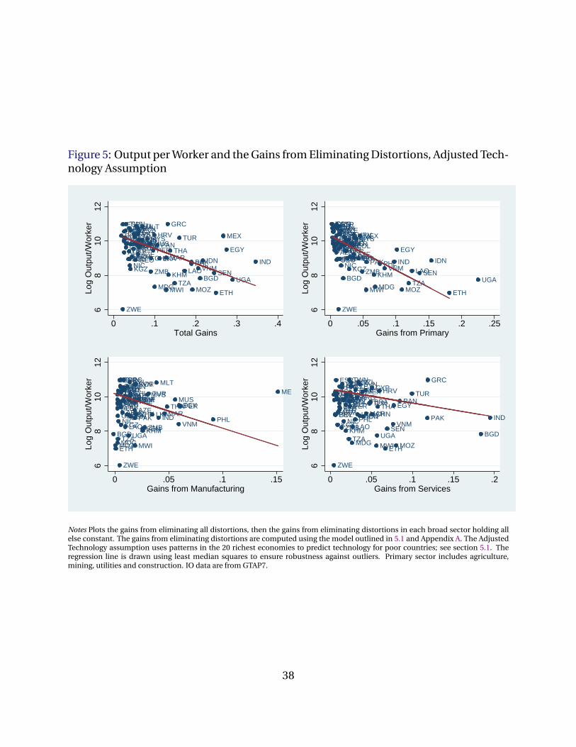
Figure 5: Output per Worker and the Gains from Eliminating Distortions, Adjusted Tech-nology Assumption

ALB

ARG

ARMAZE

BGD

BLR

BOL

BRABWACHL

CHN

COLCRI

CYPCZE

ECU EGY

ESP

EST

ETH

GEO

GRC

GTM

HRVHUN

IDN IND

IRNKAZ

KGZKHM

KOR

LAO

LKA

LTULVA

MAR

MDG

MEXMLT

MOZ

MUS

MWI

MYS

NIC

NZL

PAK

PANPER

PHL

POLPRT

PRY

ROMRUS

SEN

SVKSVN

THATUNTUR

TWN

TZA UGA

UKRURYVEN

VNM

ZAF

ZMB

ZWE68

1012

Log

Out

put/W

orke

r

0 .1 .2 .3 .4Total Gains

ALB

ARG

ARMAZE

BGD

BLR

BOL

BRABWACHL

CHN

COLCRICYPCZE

ECU EGY

ESP

EST

ETH

GEO

GRC

GTM

HRVHUN

IDNIND

IRNKAZ

KGZKHM

KOR

LAO

LKA

LTULVA

MAR

MDG

MEXMLT

MOZ

MUS

MWI

MYS

NIC

NZL

PAK

PANPER

PHL

POLPRT

PRY

ROMRUS

SEN

SVKSVN

THATUNTUR

TWN

TZA UGA

UKRURYVEN

VNM

ZAF

ZMB

ZWE68

1012

Log

Out

put/W

orke

r

0 .05 .1 .15 .2 .25Gains from Primary

ALB

ARG

ARMAZE

BGD

BLR

BOL

BRABWACHL

CHN

COLCRI

CYPCZE

ECU EGY

ESP

EST

ETH

GEO

GRC

GTM

HRVHUN

IDN IND

IRNKAZ

KGZKHM

KOR

LAO

LKA

LTULVA

MAR

MDG

MEXMLT

MOZ

MUS

MWI

MYS

NIC

NZL

PAK

PANPER

PHL

POLPRT

PRY

ROMRUS

SEN

SVKSVN

THATUNTUR

TWN

TZAUGA

UKRURYVEN

VNM

ZAF

ZMB

ZWE68

1012

Log

Out

put/W

orke

r

0 .05 .1 .15Gains from Manufacturing

ALB

ARG

ARMAZE

BGD

BLR

BOL

BRABWACHL

CHN

COLCRI

CYPCZE

ECU EGY

ESP

EST

ETH

GEO

GRC

GTM

HRVHUN

IDN IND

IRNKAZ

KGZKHM

KOR

LAO

LKA

LTULVA

MAR

MDG

MEXMLT

MOZ

MUS

MWI

MYS

NIC

NZL

PAK

PANPER

PHL

POLPRT

PRY

ROMRUS

SEN

SVKSVN

THATUNTUR

TWN

TZA UGA

UKRURYVEN

VNM

ZAF

ZMB

ZWE68

1012

Log

Out

put/W

orke

r

0 .05 .1 .15 .2Gains from Services

Notes Plots the gains from eliminating all distortions, then the gains from eliminating distortions in each broad sector holding allelse constant. The gains from eliminating distortions are computed using the model outlined in 5.1 and Appendix A. The AdjustedTechnology assumption uses patterns in the 20 richest economies to predict technology for poor countries; see section 5.1. Theregression line is drawn using least median squares to ensure robustness against outliers. Primary sector includes agriculture,mining, utilities and construction. IO data are from GTAP7.

38

Table 1: Panel: Observations by Region and Time Period

Africa Asia Latin Eastern Europe Western Europe

America & Transition & Offshoots

1950 0 0 2 0 0

1955 0 0 3 0 7

1960 0 1 4 0 4

1965 2 1 0 1 14

1970 5 7 5 0 15

1975 3 5 2 2 12

1980 1 3 1 0 6

1985 1 4 1 0 8

1990 1 4 0 0 10

1995 8 14 8 9 20

2000 15 17 14 18 19

Notes Eastern Europe and Transition includes the former Soviet republics of Armenia, Azerbaijan,Georgia, Kazakhstan and Kyrgyzstan, along with Turkey and Eastern Europe as conventionally defined.Western European “Offshoots” include Australia, Canada, Israel, New Zealand and the United States.

39

Table 2: IO coefficient means and correlations, GTAP7

Panel A: Means and standard deviations

Using Sector

Primary Sector Manufacturing Services

Pro

du

cin

gSe

cto

r

Primary Sector 0.11 0.14 0.04

(0.06) (0.11) (0.04)

Manufacturing 0.13 0.18 0.08

(0.06) (0.08) (0.05)

Services 0.12 0.16 0.20

(0.05) (0.09) (0.07)

Panel B: Correlations with log output per worker

Pro

d.S

ec. Primary Sector 0.08 -0.55 -0.33

Manufacturing 0.53 0.34 -0.13

Services 0.38 0.06 0.46

Notes Primary sector is agriculture, mining, utilities and construction. Each country’s IO table was ag-gregated into a 3x3, then each coefficient was averaged across countries to compute the means. Stan-dard deviations in parentheses under the entries in panel A. Panel B reports the correlation coefficientof each aggregated IO entry with log output per worker.

40

Table 3: IO coefficient means and correlations, panel

Panel A: Means and standard deviations

Using Sector

Primary Sector Manufacturing Services

Pro

du

cin

gSe

cto

r

Primary Sector 0.11 0.14 0.04

(0.06) (0.08) (0.03)

Manufacturing 0.17 0.22 0.08

(0.07) (0.09) (0.04)

Services 0.16 0.12 0.17

(0.06) (0.06) (0.07)

Panel B: Correlations with log output per worker

Pro

d.S

ec. Primary Sector 0.26 -0.58 -0.15

Manufacturing 0.57 0.41 0.02

Services 0.46 -0.09 0.31

Panel C: Correlations with log output per workers, country fixed effects

Pro

d.S

ec. Primary Sector 0.01 -0.56 -0.05

Manufacturing 0.10 -0.27 -0.13

Services 0.31 0.51 0.65

Notes Primary sector is agriculture, mining, utilities and construction. Each country’s IO table was aggregatedinto a 3x3, then each coefficient was averaged across countries to compute the means. Standard deviationsin parentheses under the entries in panel A. Panel B reports the correlation coefficient of each aggregated IOentry with log output per worker. Panel C reports the correlation between the residuals from regressing y andeach IO coefficient separately on country dummies.

41

Table

4:Cro

ss-section

:Main

Regressio

nR

esults

AO

MA

OM

-MS

(1)(2)

(3)(4)

(5)(6)

(7)(8)

(9)(10)

(11)(12)

AO

M(A

OM

-MS)

1.69***1.16***

0.92***1.10***

1.32***0.77***

2.70***0.84**

0.85***1.14***

1.16***0.64**

(0.61)(0.31)

(0.28)(0.29)

(0.27)(0.24)

(0.55)(0.33)

(0.32)(0.33)

(0.31)(0.29)

Ru

leo

flaw9.02***

7.89***7.45***

6.78***-2.78**

8.61***7.15***

6.40***6.34***

-3.31**

(0.67)(0.65)

(0.62)(1.07)

(1.38)(0.77)

(0.77)(0.76)

(1.26)(1.47)

Dist.E

qu

ator

0.14***0.14***

0.17***0.16***

0.18***0.18***

0.18***0.17***

(0.04)(0.04)

(0.06)(0.05)

(0.04)(0.04)

(0.06)(0.05)

Op

enn

ess0.22***

0.24***0.30***

0.24***0.22***

0.29***

(0.07)(0.08)

(0.07)(0.06)

(0.07)(0.06)

Cen

tralPlan

nin

g-1.94

-2.24-0.22

-1.25

(2.11)(1.87)

(2.29)(1.89)

Govt.C

on

sum

ptio

n-4.99**

-2.57*-4.33**

-2.11

(1.98)(1.39)

(2.00)(1.42)

Tech.A

do

ptio

n4.84***

5.03***

(0.68)(0.72)

Ob

servation

s89

8989

8989

7689

8989

8989

76

R-sq

uared

0.090.69

0.720.73

0.750.85

0.210.66

0.710.72

0.740.85

Notes

Dep

end

ent

variable

islog(RGDPWOK)

from

the

PW

T7.0

inallsp

ecificatio

ns.

Ro

bu

ststan

dard

errors

inp

arenth

eses.R

ule

ofLaw

the

averagevalu

eover

1996-2008o

fthe

Ru

leo

fLaw

ind

exfro

mK

aufm

ann

etal.(2009).O

pen

ness

is(Imports

+Exports)/

GDP

from

the

PW

T.Cen

tralPlan

nin

gis

ad

um

my

variable

that

takesth

evalu

eo

f1

ifaco

un

tryh

asa

histo

ryo

fcen

tralplan

nin

g.Govern

men

tCo

nsu

mp

tion

isfro

mth

eP

WT.Tech

Ad

op

tion

isth

ein

dex

oftech

no

logy

ado

ptio

nco

nstru

ctedb

yC

om

inetal.(2008).***,**,*

den

ote

statisticalsignifi

cance

at1%,5%

and

10%.

42

Table 5: Cross-section: Components of Output per Worker

Dependent AOM AOM-MS Number of

variable β R2 β R2 Obs.

(1) (2) (3) (4) (5)

α1−α log

(KY

)0.08 0.20 0.16* 0.22 74

(0.09) (0.09)

log(h) 0.19** 0.72 0.14 0.71 73

(0.09) (0.09)

log(TFP ) 0.45** 0.82 0.48** 0.82 71

(0.20) (0.22)Notes Each row reports the results of using either all industries (AOM ) or manufactur-

ing and service industries only (AOM −MS) in otherwise identical regressions. De-pendent variable is shown in the left column. Robust standard errors in parentheses.***, **, * denote statistical significance at 1%, 5% and 10%. Controls include all controlsused in column 6 of Table 4.

43

Table 6: Panel: Main Regression Results

AOM AOM-MS

(1) (2) (3) (4) (5) (6) (7) (8)

AOM(MS) 1.96*** 1.15** 0.94*** 0.30** 2.46*** 2.28*** 1.28*** 0.68***

(0.40) (0.38) (0.25) (0.10) (0.18) (0.45) (0.35) (0.18)

Polity IV 1.15** 0.38 1.05** 0.39

(0.41) (0.30) (0.42) (0.27)

Openness 0.93*** 0.51*** 0.81*** 0.51***

(0.13) (0.05) (0.13) (0.05)

Govt. Cons. -5.56*** -5.24*** -5.21*** -5.27***

(0.70) (0.93) (0.70) (0.80)

R-squared 0.13 0.10 0.65 0.78 0.12 0.27 0.66 0.79

Obs. 277 240 233 233 277 240 233 233

Groups 99 62 59 59 99 62 59 59

Country FE N Y Y Y N Y Y Y

Decade Dum. N N N Y N N N Y

Notes Columns 1-4 report results using AOM , while columns 5 - 8 report results using AOM −MS from otherwise identical regressions.Dependent variable is log RGDPWOK from the PWT 7.0 in all specifications. Driscoll-Kraay (1998) standard errors in parentheses. ***, **, *denote statistical significance at 1%, 5% and 10%. For specifications with fixed effects, we report the withinR2.

44

Table 7: Robustness Checks

Row Specification Cross-section Panel

AOM AOM-MS Obs. AOM AOM-MS Obs.

1 WAOM 0.48* 0.35* 76 0.25*** 0.39*** 233

(0.26) (0.19) (0.08) (0.14)

2 Imported inputs 0.62* 0.36 76

(0.33) (0.43)

3 Drop older 0.24 0.53*** 211

observations (0.13) (0.17)

4 Drop very 0.58*** 0.59*** 70 0.29** 0.72*** 214

poor countries (0.22) (0.22) (0.10) (0.20)

5 Include only -0.17 -0.11 25 -0.01 0.26* 128

rich countries (0.10) (0.16) (0.06) (0.14)

6 Drop small AOM 0.81** 0.73* 71 0.40*** 0.79*** 207

(0.31) (0.38) (0.12) (0.19)

7 Drop very 0.77*** 0.69** 60 0.37** 0.76*** 213

open countries (0.27) (0.34) (0.12) (0.21)

8 Drop small 0.77*** 0.69** 70 0.34*** 0.66*** 207

countries (0.25) (0.31) (0.08) (0.15)

9 Median regression 0.83*** 0.74** 76 0.30 0.31 233

(0.31) (0.33) (0.22) (0.29)

10 Huber robust 0.65** 0.70** 76 0.12 0.40** 233

regression (0.28) (0.31) (0.14) (0.18)

Notes Each row reports the results of using either all industries (AOM ) or manufacturing and service industries only(AOM − MS) to calculate the average output multiplier in the panel and cross sectional specifications. Dependent variableis log(RGDPWOK) from the PWT 7.0 in all specifications. Robust standard errors in parentheses. All regressions include thecontrols used in column 6 of table 4, or column 4 of table 6 . Row 1 replaces AOM with WAOM . Row 2 includes the share ofimported inputs in total output as a regressor. Row 3 drops observations before 1970. Row 4 drops countries with output perworker less than $3,000. Row 5 drops countries with output per worker less than $36,000 ($22, 000 in the panel). Row 6 dropscountries withAOM < 1.4 orAOM −MS < 1.9, respectively (AOM < 1.45 orAOM −MS < 2.28 in the panel). Row 7 dropscountries with (imports + exports)/rgdp > 1.1. Row 8 drops countries with population less that 4 million. Row 9 reports theLAD estimate of κwith bootstrapped standard errors (1000 replications). Row 10 reports the results for Huber robust regression.***, **, * denote statistical significance at 1%, 5% and 10%.

45

Table 8: Distortions and Gains, GTAP7 Summary

Avg. Distortion Gains

US Tech Adj. Tech US Tech Adj. Tech

Mean 0.16 0.04 0.17 0.10

Median 0.16 0.06 0.10 0.06

75th pctile 0.26 0.20 0.21 0.13

90th pctile 0.40 0.32 0.38 0.21

St. Dev. 0.17 0.20 0.20 0.08

Correlation 0.75 0.39

Observations 91 71 91 71

Notes Distortions are computed for each industry and averaged across industries for eachcountry using the methods outlined in section 5.1. The Adjusted Technology assumption usespatterns in the 20 richest economies to predict technology for poor countries; see section 5.1.Statistics are based on the cross-country distribution of these average distortions. The gainsfrom eliminating distortions are computed using the model outlined in 5.1 and Appendix A.All data from GTAP7.

Table 9: Distortions and Gains, Panel Summary

Avg. Distortion Total Gains Prim. Gains Mnfg. Gains Serv. Gains

Mean 0.08 0.08 0.06 0.01 0.00

Median 0.09 0.03 0.01 0.00 0.00

75th pctile 0.21 0.07 0.05 0.01 0.02

90th pctile 0.29 0.22 0.15 0.02 0.05

St. Dev. 0.20 0.14 0.13 0.02 0.05

Time Trend -0.02 -0.02 -0.02 0.00 0.00

Notes Distortions are computed for each industry and averaged across industries for each country using the methods outlined insection 5.1. Statistics are based on the cross-country distribution of these average distortions. We use patterns in the 20 richesteconomies to predict technology for poor countries; see section 5.1. The gains from eliminating distortions are computed usingthe model outlined in 5.1 and Appendix A. The sectoral gains are computed by eliminating distortions in that sector only, holdingall else constant. The IO matrix and value added shares come from the original IO tables detailed in Table 12 in Appendix B. Capitalvalue added shares are assumed constant over time and come from GTAP7. The time trend coefficient comes from a regression ofthe gains on country fixed effects and a time trend.

46

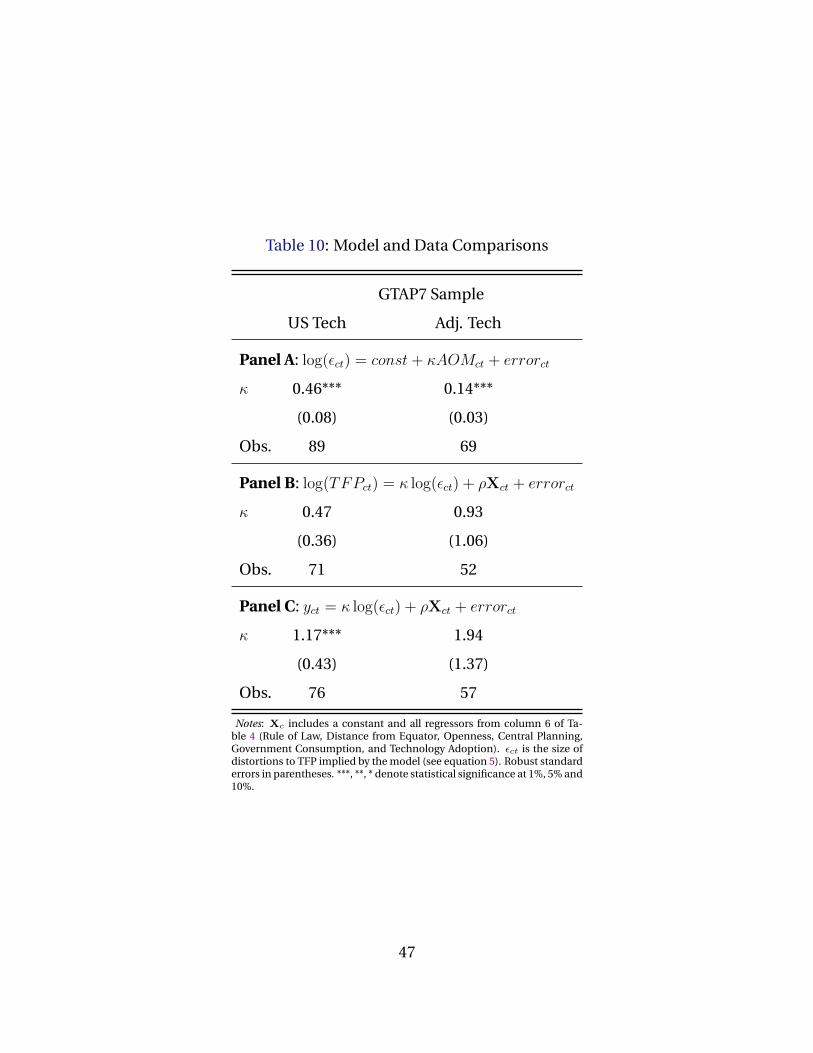
Table 10: Model and Data Comparisons

GTAP7 Sample

US Tech Adj. Tech

Panel A: log(εct) = const+ κAOMct + errorct

κ 0.46*** 0.14***

(0.08) (0.03)

Obs. 89 69

Panel B: log(TFPct) = κ log(εct) + ρXct + errorct

κ 0.47 0.93

(0.36) (1.06)

Obs. 71 52

Panel C: yct = κ log(εct) + ρXct + errorct

κ 1.17*** 1.94

(0.43) (1.37)

Obs. 76 57

Notes: Xc includes a constant and all regressors from column 6 of Ta-ble 4 (Rule of Law, Distance from Equator, Openness, Central Planning,Government Consumption, and Technology Adoption). εct is the size ofdistortions to TFP implied by the model (see equation 5). Robust standarderrors in parentheses. ***, **, * denote statistical significance at 1%, 5% and10%.

47

7 Appendices: Not for publication

A Derivations

A.1 One-Sector Growth Model with Intermediate Goods

This section presents a one sector Ramsey model with intermediate products. Gross output is

given by

Y (t) =(K(t)αL(t)1−α

)1−σX(t)σ (10)

where X is the amount of intermediate goods used in production. At any point in time compet-

itive firms solve

maxK(t),L(t),X(t)

(1− τY )(K(t)α(A(t)L(t))1−α)1−σX(t)σ − w(t)L(t)− r(t))K(t)− (1 + τX)X(t) (11)

where τY is a distortion that acts as a sales tax and τX is a distortion that acts as a tax on inter-

mediate purchases. Firm optimization implies that, at any point in time, gross output is given

by

Y (t) = K(t)αL(t)1−α[A1−α

(στ

) σ1−σ]

(12)

and net output or GDP is

Y (t)−X(t) = Y (t)(

1− σ

τ

)= K(t)αL(t)1−α

[A1−α

(στ

) σ1−σ

(1− σ

τ

)](13)

where τ = 1+τX1−τY is the “net tax rate” and the term in brackets equals the Solow residual or mea-

sured TFP. Note that, given fixed capital and labor stocks, there is no distinction between the

effects of sales taxes and taxes on intermediates.

We now establish the comparative statics of TFP at any point in time with respect to τ . Let

G = A1−α(στ

) σ1−σ

We can then derive

∂TFP

∂τ= G

[σ(1− τ)

τ2(1− σ)

]

< 0 if τ > 1

= 0 if τ = 1

> 0 if τ < 1

(14)

48

∂2TFP

∂σ∂τ= G

1− ττ4(1− σ)2

[τ2 − σ(1− σ)(1− τ) + σ(τ − σ) log(σ/τ)

](15)

< 0 if τ > 1

= 0 if τ = 1

> 0 if τ < 1

Higher taxes on intermediates, direct (τX) or indirect (τX), reduce intermediate usage from

its optimal level and lower measured TFP. A higher intermediate share implies that intermediates

are relatively more important in the production process, so distortions to intermediate inputs

(i.e. deviations from τ = 1) are more costly.

We add a household sector in order to study how intermediate goods and distortions affect

the steady state level of capital stock. Suppose a representative consumer solves

maxc(t)

∫ ∞t=0

e−ρtC(t)1−θ

1− θdt (16)

s.t. a(t) = [r(t)− δ] a(t) + w(t) + τY y(t) + τXx(t)− c(t) (17)

where lowercase variables are per capita values and δ is the capital depreciation rate. Technology

A grows at a constant exogenous rate g.

Letting k = K/AL, c = c/A and x = X/AL we can express the two dynamic equations of the

model as

˙c

c=r(t)− ρ− δ

θ− g (18)

k = kα (σ/τ)σ

1−σ [(1− τY )(1− σ) + τY + τXσ/τ ]− c− (g + δ)k (19)

where r(t) = (1 − τY )(1 − σ)αkα−1(σ/τ)σ

1−σ . Solving for the steady state value of capital per

effective labor, we find

k =

[θg + ρ+ δ

α(1− τY )(1− σ)(σ/τ)−

σ1−σ

] 1α−1

(20)

49

Along the balanced growth path, net output per worker is given by

va = Akα ·(στ

) σ1−σ

(τ − στ

)= A

[θg + ρ+ δ

α(1− τY )(1− σ)(σ/τ)−

σ1−σ

] 1α−1

·(στ

) σ1−σ

(τ − στ

)(21)

Both taxes reduce capital accumulation, but τY has a larger negative effect because it directly

reduces the rate of return on capital as well as indirectly through its effect on TFP. The effect of

net subsidies (τ < 1) on output per worker on the balanced growth path is ambiguous because

subsidies reduce TFP but encourage capital accumulation to a varying degree depending on the

specific mix of distortions.

We can establish the following:

∂ log(k)

∂τY=

1

(α− 1)(1− τY )(1− σ)< 0 (22)

∂ log(k)

∂τX=

σ

(α− 1)(1 + τX)(1− σ)< 0 (23)

The last two effects are straightforward: taxing sales and intermediates reduces the steady state

capital stock. Subsidies, on the other hand, encourage excessive capital accumulation.

A.2 Comparative Statics of σ

The comparative statics of output and productivity with respect to the factor shares in a Cobb-

Douglas production function depends crucially on whether technology augments labor/capital,

or intermediate goods/ is neutral. For example, consider the functions

F1 = A(KαLβ)1−σXσ (24)

F2 = (Kα(AL)1−α)1−σXσ (25)

and define let TFP1 and TFP2 denote total factor productivity in the value-added form of the

production function (assuming no distortions),

TFP1 = (1− σ)σσ

1−σA1

1−σ (26)

50

TFP2 = (1− σ)σσ

1−σA1−α (27)

It is easy to show that d/dσ (1−σ)σσ

1−σ < 0, which implies that dTFP2/dσ < 0. But when σ enters

into the exponent of A as in TFP1 the magnitude of A determines the sign of the derivative. For

A large enough dTFP1/dσ > 0 and forA small enough we get the opposite. These features make

conducting comparative statics with σ very unappealing since there is no good reason to prefer

one specification to another. Moreover the magnitude ofA depends on the units in which inputs

and outputs are measured, which in the case of TFP1 will affect the magnitude and sign of the

elasticity of TFP with respect to σ.

A.3 CES Generalization

Consider the CES generalization of the gross output production function (10),29

Y = (aL(πLL)ρ + aK(πKK)ρ + aX(πXX)ρ)1ρ (28)

Following the same steps as in the previous sections, in a competitive economy with distortions

the intermediate goods share will be

X

Y=

(aXπ

ρX

t

) 11−ρ

(29)

and net output will be

Y −X = constant ·1− aXπ

ρ1−ρX t

−11ρ(

1− aXπρ

1−ρX t

−ρ1ρ

) 1ρ

(30)

This expression need not be positive (or real) for all admissible values of t and ρ. Intuitively, if

the tax t is high and ρ is low the firm must pay more for its intermediate input than it can get for

its output, so production shuts down and the formula ceases to be meaningful. If t is low and ρ

is high enough the firm can make infinite profits by simply using intermediate goods to produce

final goods without the use of capital and labor at all, which also cannot be an equilibrium.

Therefore, we confine our discussion to the parameter space for which equation (30) delivers an

economically sensible answer.

We are interested in how the impact of distortions on aggregate output varies with the elas-

29This is a “normalized” CES function, appropriate for doing comparative statics on the elasticity ofsubstitution (Klump et al., 2012).

51

ticity of substitution. Intuitively, there are two off-setting effects. When the elasticity of substitu-

tion is lower, a given tax causes a relatively smaller change in the input-output coefficient (29).

On the other hand, the misallocation in input quantities induced by the distortion is more costly

the lower the elasticity of substitution. Which effect dominates depends non-monotonically on

the elasticity. Figure 6 shows the impact of different taxes for several values of the elasticity of

substitution. For an elasticity of substitution of 1/2 (i.e. ρ = −1)), the output cost of a given

level of distortion is much larger than in the case of a unit elasticity. The output cost is still larger

than in the unit elasticity case when elasticity of 1/11, but the difference is much smaller. In the

Leontief limit, the output cost of distortions is zero.

52

A.4 Multi-Sector Model

In our simulations we use the closed economy version of the multisector neoclassical growth

model with distortions explored by Jones (2011b) with 56 sectors. We refer the reader to that

paper for an in depth discussion. In this appendix we simply specify the model formally for easy

reference.

The production side of the economy consists of multiple intermediate goods sectors and a

final goods sector. Each intermediate sector has competitive input and output markets. Produc-

tion in sector i takes place using the Cobb-Douglas technology

Yi =(Kαii (AiLi)

1−αi)1−σi

·n∏j=1

Xσijij (31)

where the Xij are the intermediate goods from sector j used by sector i and σi =∑n

j=1 σij , K

is capital, L is labor, and A is the labor augmenting technology level. Firms choose input and

output levels to maximize profits:

maxKi,Li,Xij

(1− τYi )PiYi − wLi − rKi −n∑j=1

PjXij (32)

where a fraction τYi of the firm’s output is stolen and rebated lump sum to consumers. The firm’s

output is sold either to other intermediate goods producers or to the final goods sector, whose

Cobb-Douglas production function is

Y =∏i

cγii (33)

where∑

i γi = 1. Consumers then purchase this composite final good. Consumers own all

factors of production (which are in fixed supply) and care only about consumption, and since

the model is static the solution to their optimization problem is to simply spend all their income

on this consumption good.

Market clearing requires that all intermediate production is uses to produce either other in-

termediates or final goods,

Yi = ci +∑j

Xij (34)

all final good production is consumed,

Y = C (35)

53

Figure 6: Output cost of distortions for CES production functions

1 1.05 1.1 1.15 1.2 1.25 1.3 1.35 1.4 1.45 1.50.2

0.3

0.4

0.5

0.6

0.7

0.8

0.9

1

tax rate t

outp

ut

= 0 = .5 = -1 = -10

Notes The elasticity of substitution is 1/(1− ρ).

54

and all factors of production are fully employed

∑i

Ki = K (36)

∑i

Li = L (37)

A competitive equilibrium is a set of quantities C, Y, Yi,Ki, Li, Xij and prices Pi, r, w such

that all firms are maximizing profits, all markets clear and consumers consume optimally.

Jones (2011b) shows that in this competitive equilibrium aggregate output is a Cobb-Douglas

function of aggregate capital, labor and TFP, where TFP is the product of a term that involves no

distortions and a term that does, ε. In our simulations we focus on variation in ε, so we provide

the formula below.

log(ε) = ω + µ′η (38)

55

where

ω = γ′ωc + µ′ωq

µ′ = γ′(I −B∗)

ηi = log (Ai(1− τi))

ωq = ωK + ωL + ωX

ωci = log

(γiβi

)β = (I −B′)−1γ

ωXi =N∑j=1

σij log(σijβi/βj)

ωKi = δKi log(θKi)

ωLi = δLi log(θLi)

θKi =δKiβi∑N

j=1(1− τj)δKjβj

θLi =δLiβi∑N

j=1(1− τj)δLjβj

δKi = αi(1− σi)

δLi = (1− αi)(1− σi)

56

B Data Appendix

57

Table 11: Cross Section Sample of Countries

countrycode country y AOM AOM-MS

ALB Albania 9.34 1.58 1.94

ARG Argentina 9.96 1.73 2.08

ARM Armenia 9.10 1.45 1.77

AUS Australia 11.21 1.86 2.29

AUT Austria 11.19 1.80 2.29

AZE Azerbaijan 9.23 1.82 1.78

BEL Belgium 11.24 1.41 1.93

BGD Bangladesh 7.84 1.73 2.04

BLR Belarus 9.84 1.97 1.91

BOL Bolivia 8.96 1.82 2.12

BRA Brazil 9.71 1.98 2.28

CAN Canada 11.12 1.76 2.13

CHE Switzerland 11.06 1.46 2.08

CHL Chile 10.20 1.75 2.11

CHN China 9.00 2.12 2.39

COL Colombia 9.72 1.63 2.08

CRI Costa Rica 10.01 1.64 2.13

CYP Cyprus 10.53 1.51 1.99

CZE Czech Republic 10.62 2.03 2.25

DNK Denmark 11.09 1.89 2.28

ECU Ecuador 9.55 1.89 2.18

EGY Egypt 9.50 1.49 1.83

ESP Spain 10.97 1.93 2.36

EST Estonia 10.39 1.79 2.14

ETH Ethiopia 7.00 1.59 2.21

FIN Finland 11.05 1.70 2.17

FRA France 11.12 2.06 2.50

GBR United Kingdom 11.12 2.06 2.56

GEO Georgia 8.90 1.65 1.87

GER Germany 11.06 1.99 2.46

GRC Greece 10.98 1.77 2.29

58

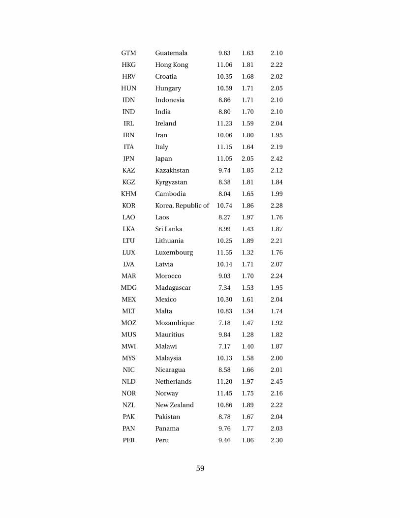
GTM Guatemala 9.63 1.63 2.10

HKG Hong Kong 11.06 1.81 2.22

HRV Croatia 10.35 1.68 2.02

HUN Hungary 10.59 1.71 2.05

IDN Indonesia 8.86 1.71 2.10

IND India 8.80 1.70 2.10

IRL Ireland 11.23 1.59 2.04

IRN Iran 10.06 1.80 1.95

ITA Italy 11.15 1.64 2.19

JPN Japan 11.05 2.05 2.42

KAZ Kazakhstan 9.74 1.85 2.12

KGZ Kyrgyzstan 8.38 1.81 1.84

KHM Cambodia 8.04 1.65 1.99

KOR Korea, Republic of 10.74 1.86 2.28

LAO Laos 8.27 1.97 1.76

LKA Sri Lanka 8.99 1.43 1.87

LTU Lithuania 10.25 1.89 2.21

LUX Luxembourg 11.55 1.32 1.76

LVA Latvia 10.14 1.71 2.07

MAR Morocco 9.03 1.70 2.24

MDG Madagascar 7.34 1.53 1.95

MEX Mexico 10.30 1.61 2.04

MLT Malta 10.83 1.34 1.74

MOZ Mozambique 7.18 1.47 1.92

MUS Mauritius 9.84 1.28 1.82

MWI Malawi 7.17 1.40 1.87

MYS Malaysia 10.13 1.58 2.00

NIC Nicaragua 8.58 1.66 2.01

NLD Netherlands 11.20 1.97 2.45

NOR Norway 11.45 1.75 2.16

NZL New Zealand 10.86 1.89 2.22

PAK Pakistan 8.78 1.67 2.04

PAN Panama 9.76 1.77 2.03

PER Peru 9.46 1.86 2.30

59

PHL Philippines 8.69 1.47 1.96

POL Poland 10.30 2.19 2.48

PRT Portugal 10.55 1.97 2.37

PRY Paraguay 8.97 1.76 2.18

ROM Romania 9.82 1.66 2.03

RUS Russia 10.08 1.98 2.17

SEN Senegal 8.15 1.33 1.86

SGP Singapore 11.28 1.44 1.96

SVK Slovak Republic 10.40 1.89 2.26

SVN Slovenia 10.73 1.86 2.29

SWE Sweden 11.13 2.06 2.49

THA Thailand 9.44 1.63 2.03

TUN Tunisia 9.63 1.56 1.98

TUR Turkey 10.19 1.54 2.02

TWN Taiwan 10.99 1.71 2.13

TZA Tanzania 7.56 1.68 2.01

UGA Uganda 7.75 1.33 1.78

UKR Ukraine 9.41 1.94 2.04

URY Uruguay 9.83 1.47 1.88

USA United States 11.33 1.93 2.31

VEN Venezuela 9.86 1.69 2.11

VNM Vietnam 8.42 1.45 1.87

ZAF South Africa 9.85 2.14 2.53

ZMB Zambia 8.22 1.66 2.07

Sources: Penn World Tables 7.0, GTAP7 at https://www.gtap.agecon.purdue.edu

60

Table 12: Non-GTAP7 Countries and Sources

Country years Source In Sample?

Argentina 1950, 1953,1959, 1963,1970

United Nations Economic Commissionfor Latin America, Tablas de insumo-producto en America Latina, Santiago deChile : Naciones Unidas, 1983

Yes

Argentina 1997 OECD, GTAP5 Yes

Australia 1968, 1974,1986, 1989,1994, 1998,2004

OECD, GTAP5 Yes

Austria 1961, 1964,1976

Economic Commission for Europe, Stan-dardized input-output tables of ECEcountries ..., New York, United Nations,various years

Yes

Austria 1995, 1997,2000, 2004

OECD, GTAP5 Yes

Burundi 1970 UNIDO, Input-output tables for develop-ing countries, New York : United Nations,1985

Yes

Belgium 1959, 1965,1970

Economic Commission for Europe, Stan-dardized input-output tables of ECEcountries ..., New York, United Nations,various years

Yes

Belgium 1995, 2000,2004

OECD, GTAP5 Yes

Bangladesh 1962 UNIDO, Input-output tables for develop-ing countries, New York : United Nations,1985

Yes

Bangladesh 1997 GTAP5 Yes

Bulgaria 1963 Economic Commission for Europe, Stan-dardized input-output tables of ECEcountries for years around 1959, NewYork, United Nations, 1972

Yes

Bolivia 1958 United Nations Economic Commissionfor Latin America, Tablas de insumo-producto en America Latina, Santiago deChile : Naciones Unidas, 1983

Yes

Botswanna 1997 GTAP5 Yes

61

Brazil 1959 United Nations Economic Commissionfor Latin America, Tablas de insumo-producto en America Latina, Santiago deChile : Naciones Unidas, 1983

No, no domesticgross output

Brazil 1970 United Nations Economic Commissionfor Latin America, Tablas de insumo-producto en America Latina, Santiago deChile : Naciones Unidas, 1983

Yes

Brazil 1995, 1996,1997, 2000,2005

OECD, GTAP5 Yes

Canada 1965, 1971,1975

Economic Commission for Europe, Stan-dardized input-output tables of ECEcountries ..., New York, United Nations,various years

Yes

Canada 1976, 1981,1986, 1990,1995, 1997,2000

OECD, GTAP5 Yes

Switzerland 2001 OECD, GTAP5 Yes

Chile 1962 United Nations Economic Commissionfor Latin America, Tablas de insumo-producto en America Latina, Santiago deChile : Naciones Unidas, 1983

Yes

Chile 1977 UNIDO, Input-output tables for develop-ing countries, New York : United Nations,1985

Yes

Chile 1986, 1996,1997

http://www.bcentral.cl, GTAP5 Yes

China 1995, 1997,2000, 2002

OECD, GTAP5 Yes

IvoryCoast

1976 UNIDO, Input-output tables for develop-ing countries, New York : United Nations,1985

No, trade marginsexcluded

IvoryCoast

1981 UNIDO, Input-output tables for develop-ing countries, New York : United Nations,1985

No, major errors

Congo 1967 UNIDO, Input-output tables for develop-ing countries, New York : United Nations,1985

No, trade marginsexcluded

Columbia 1953 United Nations Economic Commissionfor Latin America, Tablas de insumo-producto en America Latina, Santiago deChile : Naciones Unidas, 1983

No, missing servicesectors

62

Columbia 1956 United Nations Economic Commissionfor Latin America, Tablas de insumo-producto en America Latina, Santiago deChile : Naciones Unidas, 1983

Yes

Columbia 1960 United Nations Economic Commissionfor Latin America, Tablas de insumo-producto en America Latina, Santiago deChile : Naciones Unidas, 1983

No, missing servicesectors

Columbia 1970 United Nations Economic Commissionfor Latin America, Tablas de insumo-producto en America Latina, Santiago deChile : Naciones Unidas, 1983

No, trade andtransport marginsexcluded

Columbia 1997 GTAP5 Yes

Costa Rica 1957 United Nations Economic Commissionfor Latin America, Tablas de insumo-producto en America Latina, Santiago deChile : Naciones Unidas, 1983

No, missing servicesectors

Costa Rica 1972 United Nations Economic Commissionfor Latin America, Tablas de insumo-producto en America Latina, Santiago deChile : Naciones Unidas, 1983

No, missing miningsectors

Czechoslovakia1962, 1967,1973, 1977

Economic Commission for Europe, Stan-dardized input-output tables of ECEcountries ..., New York, United Nations,various years

Yes

Czech Re-public

1995, 2000,2005

OECD Yes

Denmark 1966-2005,annual

http://www.dst.dk, GTAP5 Yes

DominicanRepublic

1962 United Nations Economic Commissionfor Latin America, Tablas de insumo-producto en America Latina, Santiago deChile : Naciones Unidas, 1983

No, missing servicesectors

Ecuador 1972, 1975 United Nations Economic Commissionfor Latin America, Tablas de insumo-producto en America Latina, Santiago deChile : Naciones Unidas, 1983

No, trade marginsexcluded

Egypt 1973 UNIDO, Input-output tables for develop-ing countries, New York : United Nations,1985

No, trade marginsexcluded

Spain 1966, 1975 Economic Commission for Europe, Stan-dardized input-output tables of ECEcountries ..., New York, United Nations,various years

Yes

63

Spain 1995, 1997,2000, 2004,2005

OECD, GTAP5. Eurostat Yes

Estonia 1997, 2000,2005

OECD Yes

Finland 1965, 1970 Economic Commission for Europe, Stan-dardized input-output tables of ECEcountries ..., New York, United Nations,various years

Yes

Finland 1995-2007,annual

Eurostat, GTAP5 Yes

Fiji 1972 UNIDO, Input-output tables for develop-ing countries, New York : United Nations,1985

Yes

France 1959,1965,1970, 1975

Economic Commission for Europe, Stan-dardized input-output tables of ECEcountries ..., New York, United Nations,various years

Yes

France 1972, 1977,1980, 1985,1990, 1995-2007

OECD, GTAP5, Eurostat Yes

UnitedKingdom

1963 Economic Commission for Europe, Stan-dardized input-output tables of ECEcountries for years around 1959, NewYork, United Nations, 1972

No, major errors

UnitedKingdom

1968, 1969,1975

Economic Commission for Europe, Stan-dardized input-output tables of ECEcountries ..., New York, United Nations,various years

Yes

UnitedKingdom

1979, 1984,1990, 1995,1997, 1998,2000, 2003

OECD, GTAP5, Eurostat Yes

Germany 1959, 1965,1970, 1975

Economic Commission for Europe, Stan-dardized input-output tables of ECEcountries ..., New York, United Nations,various years

Yes

Germany 1978, 1986,1988, 1990,1995, 1997,2000-2007

OECD, GTAP5, Eurostat Yes

Ghana 1968 UNIDO, Input-output tables for develop-ing countries, New York : United Nations,1985

Yes

64

Greece 1958, 1970 Economic Commission for Europe, Stan-dardized input-output tables of ECEcountries ..., New York, United Nations,various years

Yes

Greece 1994, 1995,1997, 1999,200, 2005

OECD, GTAP5, Eurostat Yes

Guatamala 1971 United Nations Economic Commissionfor Latin America, Tablas de insumo-producto en America Latina, Santiago deChile : Naciones Unidas, 1983

Yes

Haiti 1971 United Nations Economic Commissionfor Latin America, Tablas de insumo-producto en America Latina, Santiago deChile : Naciones Unidas, 1983

No, missing domes-tic gross output

Haiti 1975 United Nations Economic Commissionfor Latin America, Tablas de insumo-producto en America Latina, Santiago deChile : Naciones Unidas, 1983

Yes

HongKong

1997 GTAP5

Hungary 1959 Economic Commission for Europe, Stan-dardized input-output tables of ECEcountries for years around 1959, NewYork, United Nations, 1972

No, missing domes-tic gross output

Hungary 1965, 1976 Economic Commission for Europe, Stan-dardized input-output tables of ECEcountries ..., New York, United Nations,various years

Yes

Hungary 1997, 1998,2000, 2005

OECD, GTAP5 Yes

Indonesia 1971 Biro Pusat Statistik, Tabel Input-OutputIndonesia, 1971

No, missing domes-tic gross output

Indonesia 1975 UNIDO, Input-output tables for develop-ing countries, New York : United Nations,1985

Yes

Indonesia 1980 Biro Pusat Statistik, Tabel Input-OutputIndonesia, 1980

No, missing domes-tic gross output

Indonesia 1985, 1998,2005

Biro Pusat Statistik, Tabel Input-OutputIndonesia, various years

Yes

Indonesia 1995, 1997,2000

OECD, GTAP5 Yes

65

India 1973 UNIDO, Input-output tables for develop-ing countries, New York : United Nations,1985

Yes

India 1993, 1997,1998, 2003

OECD, GTAP5 Yes

Ireland 1964, 1969 Economic Commission for Europe, Stan-dardized input-output tables of ECEcountries ..., New York, United Nations,various years

Yes

Ireland 1997, 1998,2000, 2005

OECD, GTAP5 Yes

Iran 2001 http://www.amar.org.ir Yes

Israel 1968, 1972 David Chen, Input-output tables 1968/69,Jerusalem : Bureau of Stats, 1975, 1979

Yes

Israel 1995, 2004 OECD Yes

Italy 1959, 1965,1970, 1975

Economic Commission for Europe, Stan-dardized input-output tables of ECEcountries ..., New York, United Nations,various years

Yes

Italy 1985, 1992,1995, 1997,2000, 2004,2005

OECD, GTAP5, Eurostat Yes

Japan 1960 Economic Commission for Europe, Stan-dardized input-output tables of ECEcountries for years around 1959, NewYork, United Nations, 1972

No, missing domes-tic gross output

Japan 1965, 1970,1975

Economic Commission for Europe, Stan-dardized input-output tables of ECEcountries ..., New York, United Nations,various years

Yes

Japan 1980, 1985,1990, 1995,1996, 1997,2000, 205

OECD, GTAP5 Yes

Kenya 1967,1971,1976

Input/Output Table for Kenya, CentralBurea of Statistics, various years

Yes

Korea 1970, 1973,1975, 1978,1980, 1983,1985-1988,1990, 1993,1995, 1998,2000, 2003,2005

Bank of Korea, GTAP5 Yes

66

Sri Lanka 1997 GTAP5 Yes

Lithuania 2000, 2005 OECD Yes

Luxembourg 1995, 1997,2000, 2005

OECD, GTAP5 Yes

Latvia 1996, 1998 OECD Yes

Morocco 1975 UNIDO, Input-output tables for develop-ing countries, New York : United Nations,1985

Yes

Morocco 1997 GTAP5 Yes

Madagascar 1973 UNIDO, Input-output tables for develop-ing countries, New York : United Nations,1985

No, missing tradeand transport

Mexico 1950, 1960 United Nations Economic Commissionfor Latin America, Tablas de insumo-producto en America Latina, Santiago deChile : Naciones Unidas, 1983

Yes

Mexico 1970, 1980 Banco de Mexico Yes

Mexico 19,972,003 OECD, GTAP5 Yes

Macedonia 2005 OECD Yes

Malta 1971 UNIDO, Input-output tables for develop-ing countries, New York : United Nations,1985

Yes

Malaysia 1978, 1983,1987, 1991

Jadual input-output Malaysia, KualaLumpur : Jabatan Perangkaan, variousyears

Yes

Malaysia 1997 GTAP5 Yes

Malawwi 1997 GTAP5 Yes

Mozambique199 GTAP5 Yes

Nicaragua 1974 UNIDO, Input-output tables for develop-ing countries, New York : United Nations,1985

Yes

Netherlands 1959, 1965,1970, 1975

Economic Commission for Europe, Stan-dardized input-output tables of ECEcountries ..., New York, United Nations,various years

Yes

Netherlands 1972, 1977,1981, 1986,1995-2005

OECD, GTAP5, Eurostat Yes

Norway 1959, 1965,1970, 1975

Economic Commission for Europe, Stan-dardized input-output tables of ECEcountries ..., New York, United Nations,various years

Yes

67

Norway 1992-2005 Eurostat Yes

Norway 1995, 2000 OECD Yes

NewZealand

1995, 1997,2002

OECD, GTAP5 Yes

Peru 1955, 1963,1968

United Nations Economic Commissionfor Latin America, Tablas de insumo-producto en America Latina, Santiago deChile : Naciones Unidas, 1983

Yes

Peru 1997 GTAP5 Yes

Philippines 1974 UNIDO, Input-output tables for develop-ing countries, New York : United Nations,1985

No, missing domes-tic gross output

Philippines 1997 GTAP5

PapuaNewGuineau

1972 UNIDO, Input-output tables for develop-ing countries, New York : United Nations,1985

Yes

Poland 1962, 1967,1977

Economic Commission for Europe, Stan-dardized input-output tables of ECEcountries ..., New York, United Nations,various years

Yes

Poland 1995, 1997,2000, 2004,205

OECD, GTAP5 Yes

Portugal 1959, 1965,1970, 1974

Economic Commission for Europe, Stan-dardized input-output tables of ECEcountries ..., New York, United Nations,various years

Yes

Portugal 1995, 1997,1999, 2000,2005

OECD, GTAP5, Eurostat Yes

Romania 2000, 2003-2005

Eurostat Yes

Russia 1995, 2000 OECD Yes

Russia 2002 OECD No, major errors

Rwanda 1970 UNIDO, Input-output tables for develop-ing countries, New York : United Nations,1985

Yes

Senegal 1959 UNIDO, Input-output tables for develop-ing countries, New York : United Nations,1985

Yes

Singapore 1973 UNIDO, Input-output tables for develop-ing countries, New York : United Nations,1985

Yes

68

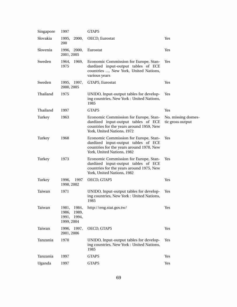
Singapore 1997 GTAP5

Slovakia 1995, 2000,200

OECD, Eurostat Yes

Slovenia 1996, 2000,2001, 2005

Eurostat Yes

Sweden 1964, 1969,1975

Economic Commission for Europe, Stan-dardized input-output tables of ECEcountries ..., New York, United Nations,various years

Yes

Sweden 1995, 1997,2000, 2005

GTAP5, Eurostat Yes

Thailand 1975 UNIDO, Input-output tables for develop-ing countries, New York : United Nations,1985

Yes

Thailand 1997 GTAP5 Yes

Turkey 1963 Economic Commission for Europe, Stan-dardized input-output tables of ECEcountries for the years around 1959, NewYork, United Nations, 1972

No, missing domes-tic gross output

Turkey 1968 Economic Commission for Europe, Stan-dardized input-output tables of ECEcountries for the years around 1970, NewYork, United Nations, 1982

Yes

Turkey 1973 Economic Commission for Europe, Stan-dardized input-output tables of ECEcountries for the years around 1975, NewYork, United Nations, 1982

Yes

Turkey 1996, 19971998, 2002

OECD, GTAP5 Yes

Taiwan 1971 UNIDO, Input-output tables for develop-ing countries, New York : United Nations,1985

Yes

Taiwan 1981, 1984,1986, 1989,1991, 1994,1999, 2004

http://eng.stat.gov.tw/ Yes

Taiwan 1996, 1997,2001, 2006

OECD, GTAP5 Yes

Tanzania 1970 UNIDO, Input-output tables for develop-ing countries, New York : United Nations,1985

Yes

Tanzania 1997 GTAP5 Yes

Uganda 1997 GTAP5 Yes

69

Uruguay 1961 United Nations Economic Commissionfor Latin America, Tablas de insumo-producto en America Latina, Santiago deChile : Naciones Unidas, 1983

No, missing miningsectors

Uruguay 1997 GTAP5 Yes

UnitedStates

1958, 1963 Economic Commission for Europe, Stan-dardized input-output tables of ECEcountries ..., New York, United Nations,various years

No, missing domes-tic gross output

UnitedStates

1972, 1977,1982

BEA Yes

UnitedStates

1985, 1990,1995, 1997,2000, 2005

OECD, GTAP5 Yes

USSR 1966 Economic Commission for Europe, Stan-dardized input-output tables of ECEcountries for the years around 1965, NewYork, United Nations, 1977

No, missing domes-tic gross output andF vector

Venezuela 1997 GTAP5 Yes

Vietnam 1997 GTAP5 Yes

Yugoslavia 1962, 170,1976

Economic Commission for Europe, Stan-dardized input-output tables of ECEcountries ..., New York, United Nations,various years

Yes

Yugoslavia 1966 Economic Commission for Europe, Stan-dardized input-output tables of ECEcountries for the years around 1965, NewYork, United Nations, 1977

No, missing sectors

SouthAfrica

1971, 1975,1978, 1981,1984, 1988,1989, 1993

ZAF stat Yes

SouthAfrica

2000, 2005 OECD Yes

Zambia 1973 UNIDO, Input-output tables for develop-ing countries, New York : United Nations,1985

No, missing domes-tic gross output

Zambia 1997 GTAP5 Yes

Zimbabwe 1997 GTAP5 Yes

Notes The table lists each IO table we collected (excluding those in GTAP7, which are listed above in Table 11), its source,and whether or not it is included in the sample. If not, we provide a brief description of why it was not. “Major errors”means that we discovered significant errors in the original sources that proved impossible to correct. Generally tablesthat were missing some major sectors were excluded, as were those that did not provide a measure of domestic grossoutput. GTAP5 is the major source of tables for 1997.

70

Table 13: GTAP Sectors and Abbreviations

Code Description Code Description Code Description

PDR Paddy rice OMT Meat products nec OTN Transport equip-ment nec

WHT Wheat VOL Vegetable oils andfats

ELE Electronic equip-ment

GRO Cereal grains nec MIL Dairy products OME Machinery andequipment nec

V F Vegetables, fruit,nuts

PCR Processed rice OMF Manufactures nec

OSD Oil seeds SGR Sugar ELY Electricity

C B Sugar cane, sugarbeet

OFD Food products nec GDT Gas manufacture,distribution

PFB Plant-based fibers B T Beverages and to-bacco products

WTR Water

OCR Crops nec TEX Textiles CNS Construction

CTL Bovine cattle, sheepand goats, horses

WAP Wearing apparel TRD Trade

OAP Animal productsnec

LEA Leather products OTP Transport nec

RMK Raw milk LUM Wood products WTP Water transport

WOL Wool, silk-worm co-coons

PPP Paper products,publishing

ATP Air transport

FRS Forestry P C Petroleum, coalproducts

CMN Communication

FSH Fishing CRP Chemical, rubber,plastic products

OFI Financial servicesnec

COA Coal NMMMineral productsnec

ISR Insurance

OIL Oil I S Ferrous metals OBS Business servicesnec

GAS Gas NFM Metals nec ROS Recreational andother services

OMN Minerals nec FMP Metal products OSG Public Adminis-tration, Defense,Education, Health

CMT Bovine meat prod-ucts

MVH Motor vehicles andparts

Source: https://www.gtap.agecon.purdue.edu

71