Linear’Regression’ - Carnegie Mellon School of ... · PDF file– Model •...

Linear Regression

1

Matt Gormley Lecture 5

September 14, 2016

School of Computer Science

Readings: Bishop, 3.1

10-‐601 Introduction to Machine Learning

Reminders

•  Homework 2: – Extension: due Friday (9/16) at 5:30pm

•  Recitation schedule posted on course website

2

Outline •  Linear Regression

–  Simple example – Model

•  Learning – Gradient Descent –  SGD –  Closed Form

•  Advanced Topics – Geometric and Probabilistic Interpretation of LMS –  L2 Regularization –  L1 Regularization –  Features

3

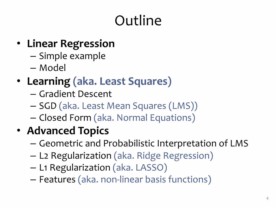
Outline •  Linear Regression

–  Simple example – Model

•  Learning (aka. Least Squares) – Gradient Descent –  SGD (aka. Least Mean Squares (LMS)) –  Closed Form (aka. Normal Equations)

•  Advanced Topics – Geometric and Probabilistic Interpretation of LMS –  L2 Regularization (aka. Ridge Regression) –  L1 Regularization (aka. LASSO) –  Features (aka. non-‐linear basis functions)

4

•  Our goal is to estimate w from a training data of <xi,yi> pairs

•  Optimization goal: minimize squared error (least squares):

•  Why least squares?

- minimizes squared distance between measurements and predicted line

- has a nice probabilistic interpretation

- the math is pretty

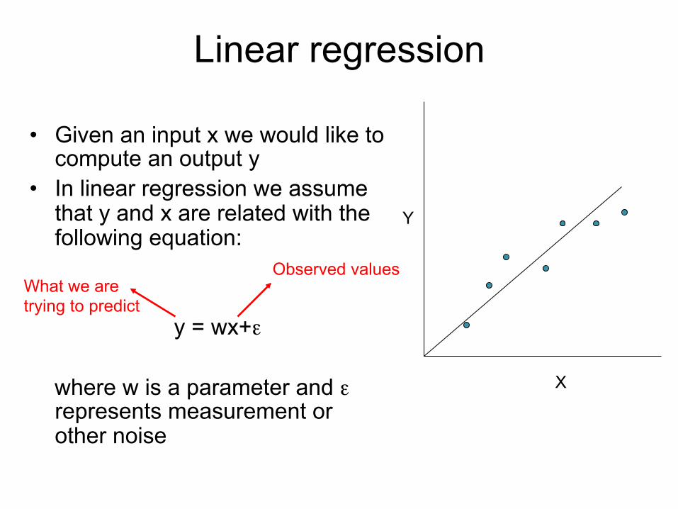
Linear regression

∑ −i

iiw wxy 2)(minargX

Y ε+= wxy

see HW

Solving linear regression

•  To optimize – closed form:

•  We just take the derivative w.r.t. to w and set to 0:

∂∂w

(yi −wxi )2

i∑ = 2 −xi (yi −wxi )

i∑ ⇒

2 xi (yi −wxi ) = 0i∑ ⇒

xiyi = wxi2

i∑

i∑ ⇒

w =xiyi

i∑

xi2

i∑

2 xiyii∑ − 2 wxixi

i∑ = 0

Linear regression

•  Given an input x we would like to compute an output y

•  In linear regression we assume that y and x are related with the following equation:

y = wx+ε where w is a parameter and ε

represents measurement or other noise

X

Y

What we are trying to predict

Observed values

Regression example

•  Generated: w=2 •  Recovered: w=2.03 •  Noise: std=1

Regression example


Bias term •  So far we assumed that the

line passes through the origin •  What if the line does not? •  No problem, simply change the

model to y = w0 + w1x+ε •  Can use least squares to

determine w0 , w1

n

xwyw i

ii∑ −=

1

0

X

Y

w0

∑

∑ −=

ii

iii

x

wyxw 2

0

1

)(

Linear Regression

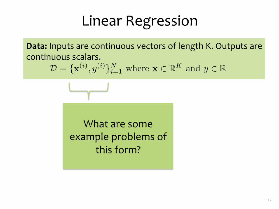
12

Data: Inputs are continuous vectors of length K. Outputs are continuous scalars.

D = {x(i), y(i)}Ni=1 where x � RK and y � R

What are some example problems of

this form?

Linear Regression

13

Data: Inputs are continuous vectors of length K. Outputs are continuous scalars.

D = {x(i), y(i)}Ni=1 where x � RK and y � R

Prediction: Output is a linear function of the inputs. y = h�(x) = �1x1 + �2x2 + . . . + �KxK

y = h�(x) = �T x (We assume x1 is 1)

Learning: finds the parameters that minimize some objective function.

�� = argmin�

J(�)

Least Squares

14

Learning: finds the parameters that minimize some objective function. We minimize the sum of the squares: Why?

1.  Reduces distance between true measurements and predicted hyperplane (line in 1D)

2.  Has a nice probabilistic interpretation

�� = argmin�

J(�)

J(�) =1

2

N�

i=1

(�T x(i) � y(i))2

Least Squares

15

Learning: finds the parameters that minimize some objective function. We minimize the sum of the squares: Why?

1.  Reduces distance between true measurements and predicted hyperplane (line in 1D)

2.  Has a nice probabilistic interpretation

�� = argmin�

J(�)

J(�) =1

2

N�

i=1

(�T x(i) � y(i))2This is a very general optimization setup. We could solve it in lots of ways. Today, we’ll consider three

ways.

Least Squares

16

Learning: Three approaches to solving

Approach 2: Stochastic Gradient Descent (SGD) (take many small steps opposite the gradient)

Approach 1: Gradient Descent (take larger – more certain – steps opposite the gradient)

Approach 3: Closed Form (set derivatives equal to zero and solve for parameters)

�� = argmin�

J(�)

Gradient Descent

17

Algorithm 1 Gradient Descent

1: procedure GD(D, �(0))2: � � �(0)

3: while not converged do4: � � � + ��J(�)

5: return �

In order to apply GD to Linear Regression all we need is the gradient of the objective function (i.e. vector of partial derivatives).

��J(�) =

�

��

dd�1

J(�)d

d�2J(�)...

dd�N

J(�)

�

��

Gradient Descent

18

Algorithm 1 Gradient Descent

1: procedure GD(D, �(0))2: � � �(0)

3: while not converged do4: � � � + ��J(�)

5: return �

There are many possible ways to detect convergence. For example, we could check whether the L2 norm of the gradient is below some small tolerance.

||��J(�)||2 � �Alternatively we could check that the reduction in the objective function from one iteration to the next is small.

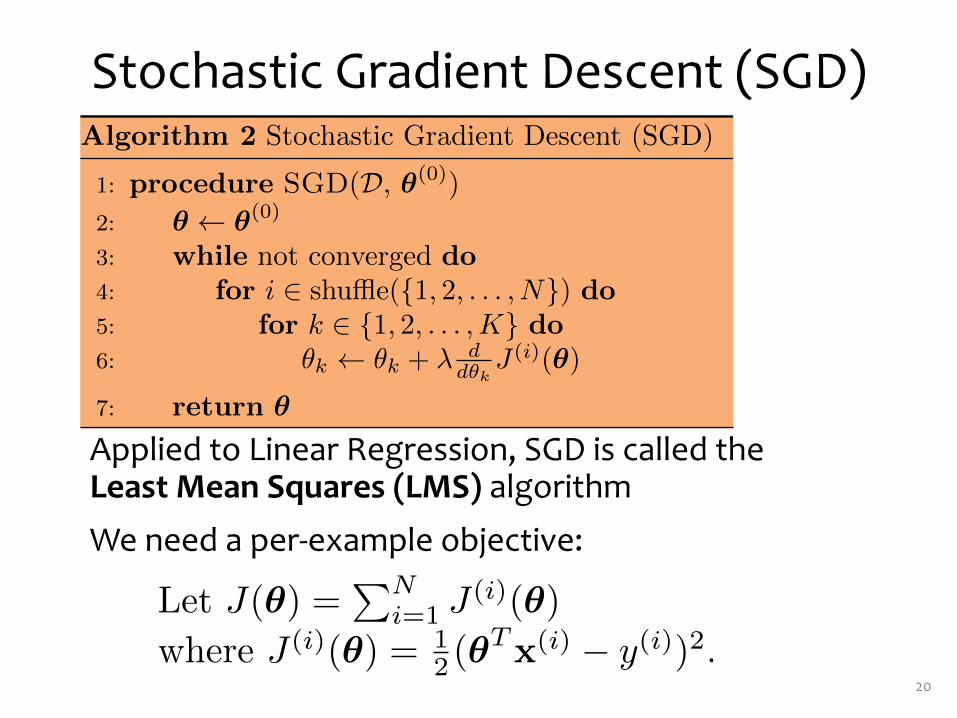
Stochastic Gradient Descent (SGD)

19

Algorithm 2 Stochastic Gradient Descent (SGD)

1: procedure SGD(D, �(0))2: � � �(0)

3: while not converged do4: for i � shu�e({1, 2, . . . , N}) do5: � � � + ��J (i)(�)

6: return �

We need a per-‐example objective:

Let J(�) =�N

i=1 J (i)(�)where J (i)(�) = 1

2 (�T x(i) � y(i))2.

Applied to Linear Regression, SGD is called the Least Mean Squares (LMS) algorithm



20

Let J(�) =�N

i=1 J (i)(�)where J (i)(�) = 1

2 (�T x(i) � y(i))2.



1: procedure SGD(D, �(0))2: � � �(0)

3: while not converged do4: for i � shu�e({1, 2, . . . , N}) do5: for k � {1, 2, . . . , K} do6: �k � �k + � d

d�kJ (i)(�)

7: return �



21

Let J(�) =�N

i=1 J (i)(�)where J (i)(�) = 1

2 (�T x(i) � y(i))2.



1: procedure SGD(D, �(0))2: � � �(0)

3: while not converged do4: for i � shu�e({1, 2, . . . , N}) do5: for k � {1, 2, . . . , K} do6: �k � �k + � d

d�kJ (i)(�)

7: return �

Let’s start by calculating this partial derivative for the Linear Regression objective function.

Partial Derivatives for Linear Reg.

22

d

d�kJ (i)(�) =

d

d�k

1

2(�T x(i) � y(i))2

=1

2

d

d�k(�T x(i) � y(i))2

= (�T x(i) � y(i))d

d�k(�T x(i) � y(i))

= (�T x(i) � y(i))d

d�k(

K�

k=1

�kx(i)k � y(i))

= (�T x(i) � y(i))x(i)k

Let J(�) =�N

i=1 J (i)(�)where J (i)(�) = 1

2 (�T x(i) � y(i))2.

Partial Derivatives for Linear Reg.

23

Let J(�) =�N

i=1 J (i)(�)where J (i)(�) = 1

2 (�T x(i) � y(i))2.

d

d�kJ (i)(�) = (�T x(i) � y(i))x(i)

k

d

d�kJ(�) =

d

d�k

N�

i=1

J (i)(�)

=N�

i=1

(�T x(i) � y(i))x(i)k

Used by SGD (aka. LMS)

Used by Gradient Descent

Least Mean Squares (LMS)

24


Algorithm 3 Least Mean Squares (LMS)

1: procedure LMS(D, �(0))2: � � �(0)

3: while not converged do4: for i � shu�e({1, 2, . . . , N}) do5: for k � {1, 2, . . . , K} do

6: �k � �k + �(�T x(i) � y(i))x(i)k

7: return �

Optimization for Linear Reg. vs. Logistic Reg.

•  Can use the same tricks for both: –  regularization –  tuning learning rate on development data –  shuffle examples out-‐of-‐core (if can’t fit in memory) and stream over them

–  local hill climbing yields global optimum (both problems are convex)

–  etc. •  But Logistic Regression does not have a closed form solution for MLE parameters… …what about Linear Regression?

25

Least Squares

26





�� = argmin�

J(�)

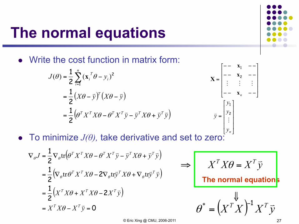
The normal equations l  Write the cost function in matrix form:

l  To minimize J(θ), take derivative and set to zero:

© Eric Xing @ CMU, 2006-2011 27

( ) ( )

( )yyXyyXXX

yXyX

yJ

TTTTTT

T

n

ii

Ti

!!!!

!!

+−−=

−−=

−= ∑=

θθθθ

θθ

θθ

212121

1

2)()( x

⎥⎥⎥⎥

⎦

⎤

⎢⎢⎢⎢

⎣

⎡

−−−−

−−−−

−−−−

=

nx

xx

X!!!

2

1

⎥⎥⎥⎥

⎦

⎤

⎢⎢⎢⎢

⎣

⎡

=

ny

yy

y!

" 2

1

( )

( )

( )0

221

22121

=−=

−+=

∇+∇−∇=

+−−∇=∇

yXXX

yXXXXX

yyXyXX

yyXyyXXXJ

TT

TTT

TTTT

TTTTTT

!

!

!!!

!!!!

θ

θθ

θθθ

θθθθ

θθθ

θθ

trtrtr

tryXXX TT !

=⇒ θ The normal equations

( ) yXXX TT !1−=*θ

⇓

Some matrix derivatives l  For , define:

l  Trace:

l  Some fact of matrix derivatives (without proof)

© Eric Xing @ CMU, 2006-2011 28

⎥⎥⎥⎥⎥⎥⎥

⎦

⎤

⎢⎢⎢⎢⎢⎢⎢

⎣

⎡

∂

∂

∂

∂

∂

∂

∂

∂

=∇

fA

fA

fA

fA

Af

mnm

n

A

!

"#"

!

1

111

)(

RR !nmf ×:

, tr ∑=

=n

iiiAA

1, tr aa = BCACABABC trtrtr ==

, tr TA BAB =∇ , tr TTT

A ABCCABCABA +=∇ ( ) TA AAA 1−=∇

Comments on the normal equation

l  In most situations of practical interest, the number of data points N is larger than the dimensionality k of the input space and the matrix X is of full column rank. If this condition holds, then it is easy to verify that XTX is necessarily invertible.

l  The assumption that XTX is invertible implies that it is positive definite, thus the critical point we have found is a minimum.

l  What if X has less than full column rank? à regularization (later).

© Eric Xing @ CMU, 2006-2011 29

Direct and Iterative methods l  Direct methods: we can achieve the solution in a single step

by solving the normal equation l  Using Gaussian elimination or QR decomposition, we converge in a finite number

of steps l  It can be infeasible when data are streaming in in real time, or of very large

amount

l  Iterative methods: stochastic or steepest gradient l  Converging in a limiting sense l  But more attractive in large practical problems l  Caution is needed for deciding the learning rate α

© Eric Xing @ CMU, 2006-2011 30

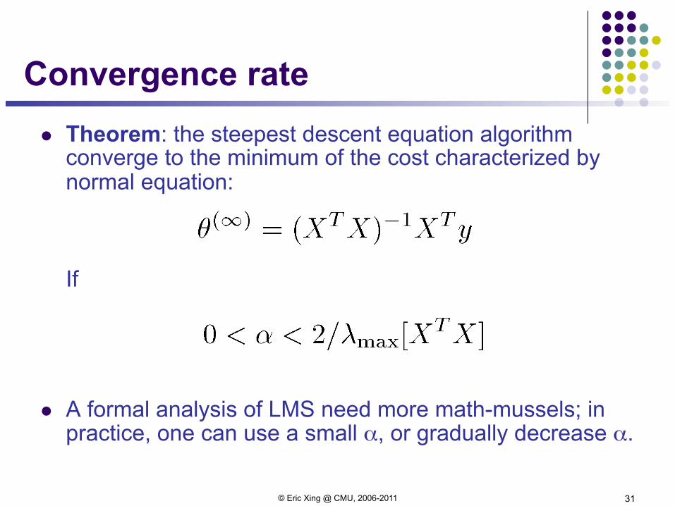
Convergence rate l  Theorem: the steepest descent equation algorithm

converge to the minimum of the cost characterized by normal equation:

If

l  A formal analysis of LMS need more math-mussels; in

practice, one can use a small α, or gradually decrease α.

© Eric Xing @ CMU, 2006-2011 31

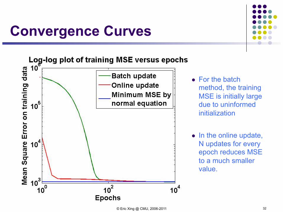
Convergence Curves

l  For the batch method, the training MSE is initially large due to uninformed initialization

l  In the online update, N updates for every epoch reduces MSE to a much smaller value.

32 © Eric Xing @ CMU, 2006-2011

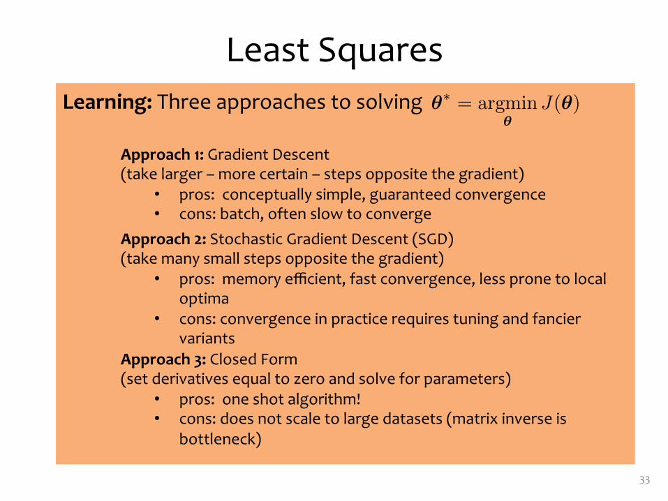
Least Squares

33



•  pros: memory efficient, fast convergence, less prone to local optima

•  cons: convergence in practice requires tuning and fancier variants


•  pros: conceptually simple, guaranteed convergence •  cons: batch, often slow to converge


•  pros: one shot algorithm! •  cons: does not scale to large datasets (matrix inverse is

bottleneck)

�� = argmin�

J(�)

Matching Game

Goal: Match the Algorithm to its Update Rule

34

1. SGD for Logistic Regression

2. Least Mean Squares

3. Perceptron (next lecture)

4.

5.

6.

A. 1=5, 2=4, 3=6 B. 1=5, 2=6, 3=4 C. 1=6, 2=4, 3=4 D. 1=5, 2=6, 3=6 E. 1=6, 2=6, 3=6

�k � �k +1

1 + exp �(h�(x(i)) � y(i))

�k � �k + (h�(x(i)) � y(i))

�k � �k + �(h�(x(i)) � y(i))x(i)k

h�(x) = p(y|x)

h�(x) = �T x

h�(x) = sign(�T x)

Geometric Interpretation of LMS •  The predictions on the training data are:

•  Note that

and is the orthogonal projection of

into the space spanned by the columns of X

( ) yXXXXXy TT !! 1−== *ˆ θ

( )( )yIXXXXyy TT !!!−=−

−1ˆ

( ) ( )( )( )( )

0

1

1

=

−=

−=−−

−

yXXXXXX

yIXXXXXyyXTTTT

TTTT

!

!!!

!!

y! y!

⎥⎥⎥⎥

⎦

⎤

⎢⎢⎢⎢

⎣

⎡

−−−−

−−−−

−−−−

=

nx

xx

X!!!

2

1

⎥⎥⎥⎥

⎦

⎤

⎢⎢⎢⎢

⎣

⎡

=

ny

yy

y!

" 2

1

35 © Eric Xing @ CMU, 2006-‐2011

Probabilistic Interpretation of LMS •  Let us assume that the target variable and the inputs

are related by the equation:

where ε is an error term of unmodeled effects or random

noise

•  Now assume that ε follows a Gaussian N(0,σ), then we have:

•  By independence assumption:

iiT

iy εθ += x

⎟⎟⎠

⎞⎜⎜⎝

⎛ −−= 2

2

221

σθ

σπθ

)(exp);|( iT

iii

yxyp x

⎟⎟

⎠

⎞

⎜⎜

⎝

⎛ −−⎟

⎠

⎞⎜⎝

⎛==

∑∏ =

=2

12

1 221

σ

θ

σπθθ

n

i iT

inn

iii

yxypL

)(exp);|()(

x

36 © Eric Xing @ CMU, 2006-‐2011

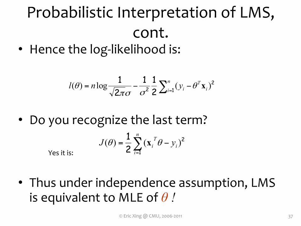
Probabilistic Interpretation of LMS, cont.

•  Hence the log-‐likelihood is:

•  Do you recognize the last term? Yes it is:

•  Thus under independence assumption, LMS is equivalent to MLE of θ !

∑ =−−=

n

i iT

iynl1

22 211

21 )(log)( xθ

σσπθ

∑=

−=n

ii

Ti yJ

1

2

21 )()( θθ x

37 © Eric Xing @ CMU, 2006-‐2011

Ridge Regression

•  Adds an L2 regularizer to Linear Regression

•  Bayesian interpretation: MAP estimation with a Gaussian prior on the parameters

38

JRR(�) = J(�) + �||�||22

=1

2

N�

i=1

(�T x(i) � y(i))2 + �K�

k=1

�2k

�MAP = argmax�

N�

i=1

log p�(y(i)|x(i)) + log p(�)

= argmax�

JRR(�)where

p(�) � N (0,1�)

�MAP = argmax�

N�

i=1

log p�(y(i)|x(i)) + log p(�)

= argmax�

JLASSO(�)

JLASSO(�) = J(�) + �||�||1

=1

2

N�

i=1

(�T x(i) � y(i))2 + �K�

k=1

|�k|

LASSO

•  Adds an L1 regularizer to Linear Regression

•  Bayesian interpretation: MAP estimation with a Laplace prior on the parameters

39

where

p(�) � Laplace(0, f(�))

Ridge Regression vs Lasso

Ridge Regression: Lasso:

Lasso (l1 penalty) results in sparse solu2ons – vector with more zero coordinates Good for high-‐dimensional problems – don’t have to store all coordinates!

βs with constant l1 norm

βs with constant J(β) (level sets of J(β))

βs with constant l2 norm

β2

β1

40 © Eric Xing @ CMU, 2006-‐2011

X X

Non-Linear basis function •  So far we only used the observed values x1,x2,… •  However, linear regression can be applied in the same

way to functions of these values –  Eg: to add a term w x1x2 add a new variable z=x1x2 so each

example becomes: x1, x2, …. z

•  As long as these functions can be directly computed from the observed values the parameters are still linear in the data and the problem remains a multi-variate linear regression problem

ε++++= 22110 kk xwxwwy …

Non-linear basis functions

•  What type of functions can we use? •  A few common examples: - Polynomial: φj(x) = xj for j=0 … n - Gaussian: - Sigmoid:

- Logs:

€

φ j (x) =(x −µ j )2σ j

2

€

φ j (x) =1

1+ exp(−s j x)

Any function of the input values can be used. The solution for the parameters of the regression remains the same.

φ j (x) = log(x +1)

General linear regression problem •  Using our new notations for the basis function linear

regression can be written as

•  Where φj(x) can be either xj for multivariate regression or one of the non-linear basis functions we defined

•  … and φ0(x)=1 for the intercept term €

y = w jφ j (x)j= 0

n

∑

An example: polynomial basis vectors on a small dataset

– From Bishop Ch 1

0th Order Polynomial

n=10

1st Order Polynomial

3rd Order Polynomial

9th Order Polynomial

Over-fitting

Root-Mean-Square (RMS) Error:

Polynomial Coefficients

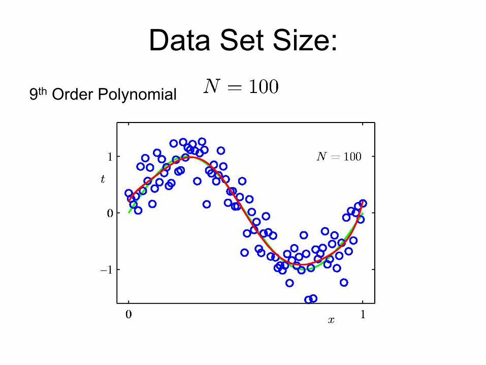
Data Set Size: 9th Order Polynomial

Regularization

Penalize large coefficient values

JX,y (w) =12

yi − wjφ j (xi )

j∑

#

$%%

&

'((

i∑

2

−λ2w 2

Regularization: +

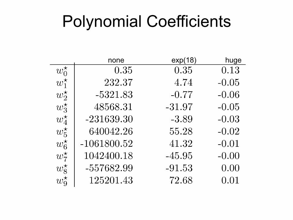
Polynomial Coefficients

none exp(18) huge

Over Regularization:

Linear’Regression’ - Carnegie Mellon School of ... · PDF file– Model •...

Documents

Transcript of Linear’Regression’ - Carnegie Mellon School of ... · PDF file– Model •...