Linearized gravity and Hadamard stateshome.mathematik.uni-freiburg.de/murro/pdf/Dijon.pdf ·...

Linearized gravity and Hadamard states

Simone Murro

Department of MathematicsUniversity of Regensburg

Séminaires Math-Physique

Dijon, 10th of May 2017

Simone Murro (Universität Regensburg) Algebraic Quantum Field Theory Dijon, 2017 1 / 20

General Framework

Is there a quantum theory of General Relativity?

1) String theory, loop quantum gravity.

2) Algebraic approach to quantum gravity.

[Brunetti, Fewster, Fredenhagen, Giesel, Majid, Rejzner, Tiemann, . . .]

Algebraic approach −→ rigorous approach to QFT

[Araki, Bär, Brunetti, Buchholz, Dappiaggi, Dimock, Finster, Fredenhagen, Gérard,Ginoux, Haag, Kay, Moretti, Pinamonti, Strohmaier, Verch, Wald, . . .]

Why is the construction of a Hadamard state important?

1) Evaluation of the influence of gravitational field on physical observables.

2) Understand in the algebraic approach structural problems of quantum gravity.[Brunetti, Fredenhagen, Rejzner: Quantum gravity from the point of view of locallycovariant quantum field theory ]


Outline

Outline

On the algebraic approach to quantum field theory

Linearized gravity on globally hyperbolic spacetimes

Hadamard states for linearized gravity on asymptotically flat spacetimes

Based on:

I M. Benini, C. Dappiaggi and S.M. - J. Math. Phys. 55 082301 (2014)


Algebraic Quantum Field Theory

PART I:

On the algebraic approachto quantum field theory



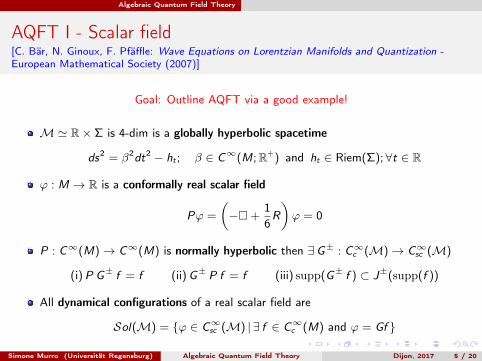
AQFT I - Scalar field[C. Bär, N. Ginoux, F. Pfäffle: Wave Equations on Lorentzian Manifolds and Quantization -European Mathematical Society (2007)]

Goal: Outline AQFT via a good example!

M' R× Σ is 4-dim is a globally hyperbolic spacetime

ds2 = β2dt2 − ht ; β ∈ C∞(M;R+) and ht ∈ Riem(Σ);∀t ∈ R

ϕ : M → R is a conformally real scalar field

Pϕ =

(−+

16R

)ϕ = 0

P : C∞(M)→ C∞(M) is normally hyperbolic then ∃G± : C∞c (M)→ C∞sc (M)

(i)P G± f = f (ii)G± P f = f (iii) supp(G± f ) ⊂ J±(supp(f ))

All dynamical configurations of a real scalar field are

Sol(M) = ϕ ∈ C∞sc (M) | ∃ f ∈ C∞c (M) and ϕ = Gf



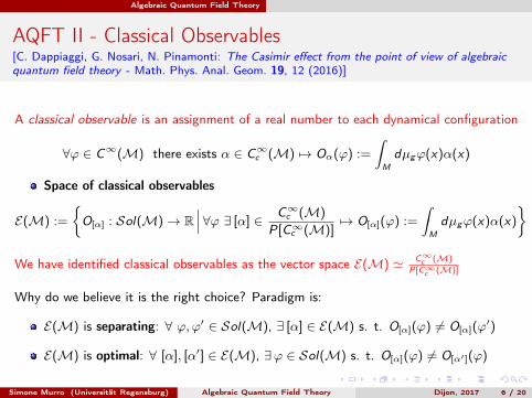
AQFT II - Classical Observables[C. Dappiaggi, G. Nosari, N. Pinamonti: The Casimir effect from the point of view of algebraicquantum field theory - Math. Phys. Anal. Geom. 19, 12 (2016)]

A classical observable is an assignment of a real number to each dynamical configuration

∀ϕ ∈ C∞(M) there exists α ∈ C∞c (M) 7→ Oα(ϕ) :=

ˆM

dµgϕ(x)α(x)

Space of classical observables

E(M) :=

O[α] : Sol(M)→ R

∣∣∣ ∀ϕ ∃ [α] ∈ C∞c (M)

P[C∞c (M)]7→ O[α](ϕ) :=

ˆM

dµgϕ(x)α(x)

We have identified classical observables as the vector space E(M) ' C∞c (M)

P[C∞c (M)]

Why do we believe it is the right choice? Paradigm is:

E(M) is separating: ∀ ϕ,ϕ′ ∈ Sol(M), ∃ [α] ∈ E(M) s. t. O[α](ϕ) 6= O[α](ϕ′)

E(M) is optimal: ∀ [α], [α′] ∈ E(M), ∃ϕ ∈ Sol(M) s. t. O[α](ϕ) 6= O[α′](ϕ)



AQFT III - Algebra of Observables[J. Dimock: Algebras of Local Observables on a Manifold - Commun. Math. Phys. 77, 219(1980)]

Gaol: From E(M;C) = E(M)⊗ C build the “algebra of fields”

(1) Construct the unital Borchers-Uhlmann ∗-algebra:

A =∞⊕n=0

E(M;C)⊗n

where E(M;C)0 = C and the ∗-operation is complex conjugation

(2) Construct the ideal I (M) ⊂ A (M) generated by elements of the form

[α]⊗ [α′]− [α′]⊗ [α]− ıG([α], [α′])11 ,

where 11 is the unit in A (M) and

G([α], [α′]).

=(α | Gα′

)=

ˆM

dµgα(x)G(α′)(x)

(3) Define the Algebra of Fields F (M).

= A (M)I (M)



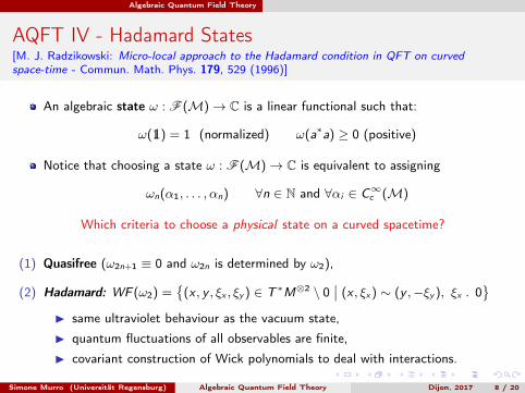
AQFT IV - Hadamard States[M. J. Radzikowski: Micro-local approach to the Hadamard condition in QFT on curvedspace-time - Commun. Math. Phys. 179, 529 (1996)]

An algebraic state ω : F (M)→ C is a linear functional such that:

ω(11) = 1 (normalized) ω(a∗a) ≥ 0 (positive)

Notice that choosing a state ω : F (M)→ C is equivalent to assigning

ωn(α1, . . . , αn) ∀n ∈ N and ∀αi ∈ C∞c (M)

Which criteria to choose a physical state on a curved spacetime?

(1) Quasifree (ω2n+1 ≡ 0 and ω2n is determined by ω2),

(2) Hadamard: WF (ω2) =

(x , y , ξx , ξy ) ∈ T ∗M⊗2 \ 0∣∣ (x , ξx) ∼ (y ,−ξy ), ξx . 0

I same ultraviolet behaviour as the vacuum state,

I quantum fluctuations of all observables are finite,

I covariant construction of Wick polynomials to deal with interactions.


Linearized gravity

PART II:

Linearized gravity onglobally hyperbolic spacetimes


Linearized gravity

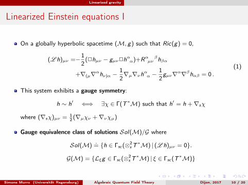
Linearized Einstein equations I

On a globally hyperbolic spacetime (M, g) such that Ric(g) = 0,

(L h)µν =−12

(2hµν − gµν2hαα)+Rα βµν hβα

+∇(µ∇αhν)α −12∇µ∇νhαα −

12gµν∇α∇βhαβ = 0 .

(1)

This system exhibits a gauge symmetry:

h ∼ h′ ⇐⇒ ∃χ ∈ Γ(T ∗M) such that h′ = h +∇sχ

where (∇sχ)µν = 12 (∇µχν +∇νχµ)

Gauge equivalence class of solutions Sol(M)/G where

Sol(M).

= h ∈ Γsc(⊗2sT∗M) | (L h)µν = 0.

G(M) = Lξg ∈ Γsc(⊗2sT∗M) | ξ ∈ Γsc(T ∗M)


Linearized gravity

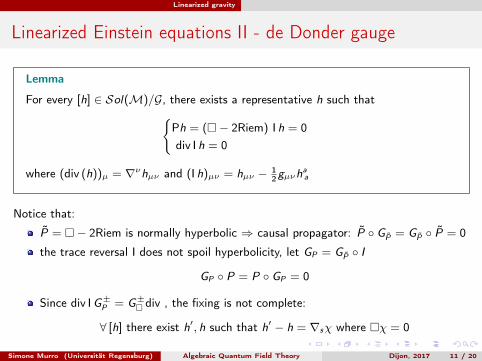
Linearized Einstein equations II - de Donder gauge

Lemma

For every [h] ∈ Sol(M)/G, there exists a representative h such thatPh = (− 2Riem) I h = 0div I h = 0

where (div (h))µ = ∇νhµν and (I h)µν = hµν − 12gµνh

aa

Notice that:

P = − 2Riem is normally hyperbolic ⇒ causal propagator: P GP = GP P = 0

the trace reversal I does not spoil hyperbolicity, let GP = GP I

GP P = P GP = 0

Since div IG±P = G± div , the fixing is not complete:

∀ [h] there exist h′, h such that h′ − h = ∇sχ where χ = 0


Linearized gravity

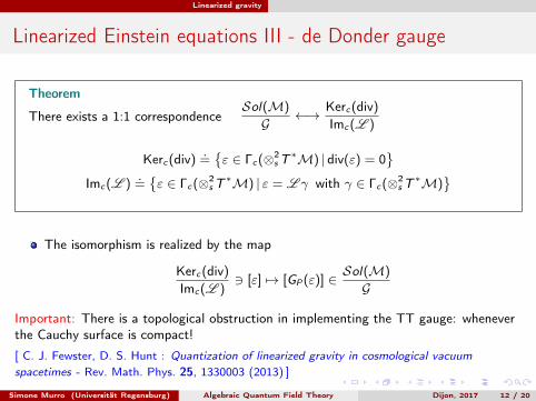
Linearized Einstein equations III - de Donder gauge

Theorem

There exists a 1:1 correspondenceSol(M)

G ←→ Kerc(div)Imc(L )

Kerc(div).

=ε ∈ Γc(⊗2

sT∗M) | div(ε) = 0

Imc(L )

.=ε ∈ Γc(⊗2

sT∗M) | ε = L γ with γ ∈ Γc(⊗2

sT∗M)

The isomorphism is realized by the map

Kerc(div)Imc(L )

3 [ε] 7→ [GP(ε)] ∈ Sol(M)

G

Important: There is a topological obstruction in implementing the TT gauge: wheneverthe Cauchy surface is compact!

[ C. J. Fewster, D. S. Hunt : Quantization of linearized gravity in cosmological vacuumspacetimes - Rev. Math. Phys. 25, 1330003 (2013) ]


Linearized gravity

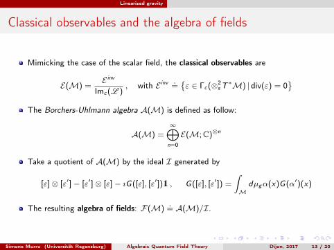
Classical observables and the algebra of fields

Mimicking the case of the scalar field, the classical observables are

E(M) =E inv

Imc(L ), with E inv .

=ε ∈ Γc(⊗2

sT∗M) | div(ε) = 0

The Borchers-Uhlmann algebra A(M) is defined as follow:

A(M) =∞⊕n=0

E(M;C)⊗n

Take a quotient of A(M) by the ideal I generated by

[ε]⊗ [ε′]− [ε′]⊗ [ε]− ıG([ε], [ε′])11 , G([ε], [ε′]) =

ˆM

dµgα(x)G(α′)(x)

The resulting algebra of fields: F(M).

= A(M)/I.


Hadamard states

PART III:

Hadamard statesfor linearized gravity on

asymptotically flat spacetimes


Hadamard states

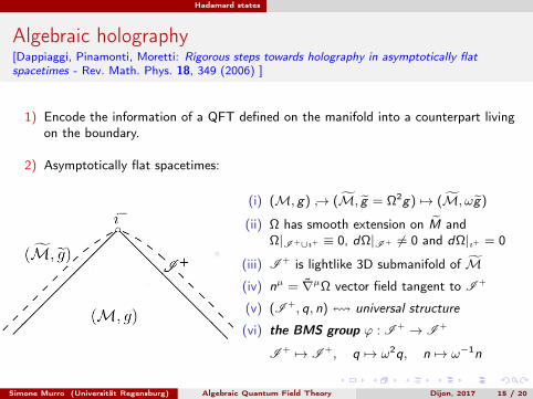
Algebraic holography[Dappiaggi, Pinamonti, Moretti: Rigorous steps towards holography in asymptotically flatspacetimes - Rev. Math. Phys. 18, 349 (2006) ]

1) Encode the information of a QFT defined on the manifold into a counterpart livingon the boundary.

2) Asymptotically flat spacetimes:

(i) (M, g) → (M, g = Ω2g) 7→ (M, ωg)

(ii) Ω has smooth extension on M andΩ|I+∪ı+ ≡ 0, dΩ|I+ 6= 0 and dΩ|ı+ = 0

(iii) I + is lightlike 3D submanifold of M(iv) nµ = ∇µΩ vector field tangent to I +

(v) (I +, q, n) ! universal structure

(vi) the BMS group ϕ : I + → I +

I + 7→ I +, q 7→ ω2q, n 7→ ω−1n


Hadamard states

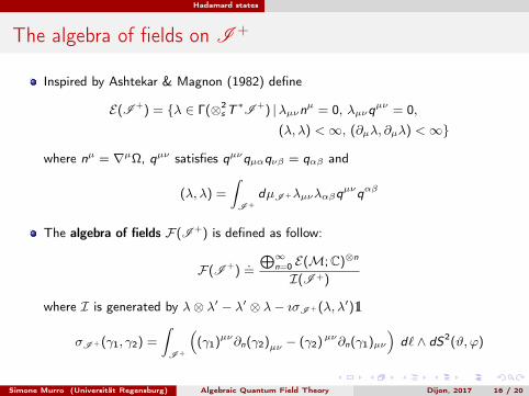
The algebra of fields on I +

Inspired by Ashtekar & Magnon (1982) define

E(I +) = λ ∈ Γ(⊗2sT∗I +) |λµνnµ = 0, λµνqµν = 0,

(λ, λ) <∞, (∂µλ, ∂µλ) <∞

where nµ = ∇µΩ, qµν satisfies qµνqµαqνβ = qαβ and

(λ, λ) =

ˆI+

dµI+λµνλαβqµνqαβ

The algebra of fields F(I +) is defined as follow:

F(I +).

=

⊕∞n=0 E(M;C)⊗n

I(I +)

where I is generated by λ⊗ λ′ − λ′ ⊗ λ− ıσI+(λ, λ′)11

σI+(γ1, γ2) =

ˆI+

((γ1)µν∂n(γ2)µν − (γ2)µν∂n(γ1)µν

)d` ∧ dS2(ϑ, ϕ)


Hadamard states

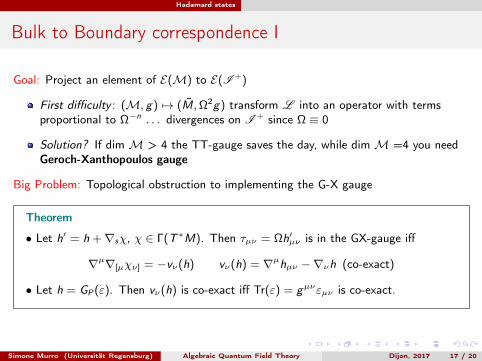
Bulk to Boundary correspondence I

Goal: Project an element of E(M) to E(I +)

First difficulty : (M, g) 7→ (M,Ω2g) transform L into an operator with termsproportional to Ω−n . . . divergences on I + since Ω ≡ 0

Solution? If dimM > 4 the TT-gauge saves the day, while dimM =4 you needGeroch-Xanthopoulos gauge

Big Problem: Topological obstruction to implementing the G-X gauge

Theorem

• Let h′ = h +∇sχ, χ ∈ Γ(T ∗M). Then τµν = Ωh′µν is in the GX-gauge iff

∇µ∇[µχν] = −vν(h) vν(h) = ∇µhµν −∇νh (co-exact)

• Let h = GP(ε). Then vν(h) is co-exact iff Tr(ε) = gµνεµν is co-exact.


Hadamard states

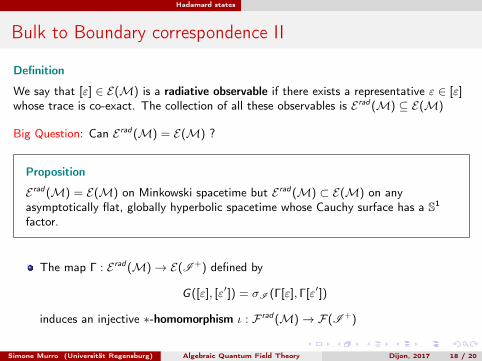
Bulk to Boundary correspondence II

Definition

We say that [ε] ∈ E(M) is a radiative observable if there exists a representative ε ∈ [ε]whose trace is co-exact. The collection of all these observables is E rad(M) ⊆ E(M)

Big Question: Can E rad(M) = E(M) ?

Proposition

E rad(M) = E(M) on Minkowski spacetime but E rad(M) ⊂ E(M) on anyasymptotically flat, globally hyperbolic spacetime whose Cauchy surface has a S1

factor.

The map Γ : E rad(M)→ E(I +) defined by

G([ε], [ε′]) = σI (Γ[ε], Γ[ε′])

induces an injective ∗-homomorphism ι : F rad(M)→ F(I +)


Hadamard states

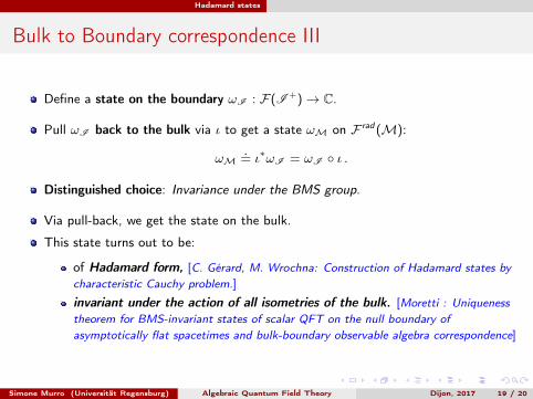
Bulk to Boundary correspondence III

Define a state on the boundary ωI : F(I +)→ C.

Pull ωI back to the bulk via ι to get a state ωM on F rad(M):

ωM.

= ι∗ωI = ωI ι .

Distinguished choice: Invariance under the BMS group.

Via pull-back, we get the state on the bulk.

This state turns out to be:

of Hadamard form, [C. Gérard, M. Wrochna: Construction of Hadamard states bycharacteristic Cauchy problem.]

invariant under the action of all isometries of the bulk. [Moretti : Uniquenesstheorem for BMS-invariant states of scalar QFT on the null boundary ofasymptotically flat spacetimes and bulk-boundary observable algebra correspondence]


Conclusions

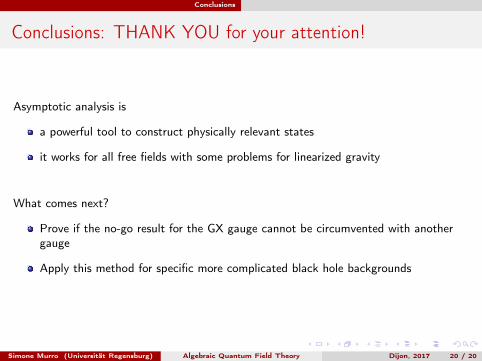
Conclusions: THANK YOU for your attention!

Asymptotic analysis is

a powerful tool to construct physically relevant states

it works for all free fields with some problems for linearized gravity

What comes next?

Prove if the no-go result for the GX gauge cannot be circumvented with anothergauge

Apply this method for specific more complicated black hole backgrounds


Linearized gravity and Hadamard stateshome.mathematik.uni-freiburg.de/murro/pdf/Dijon.pdf ·...

Documents

Transcript of Linearized gravity and Hadamard stateshome.mathematik.uni-freiburg.de/murro/pdf/Dijon.pdf ·...