Linear Viscoelasticity: Review of Theory and Applications ...

Reports in Mechanical Engineering

Vol. 2, No.1, 2021, pp. 156-179.

ISSN: 2683-5894, DOI: https://doi.org/10.31181/rme200102156m 156

Journal homepage: https://www.frontpres.rabek.org

Linear Viscoelasticity: Review of Theory and Applications in

Atomic Force Microscopy

Marshall R. McCraw1, Berkin Uluutku1 and Santiago D. Solares1

1 Department of Mechanical and Aerospace Engineering, The George Washington University, Washington, USA

Article Info ABSTRACT

Article history:

Received Jun 3, 2021

Revised July 20, 2021

Accepted July 22, 2021

Recently, much research has been performed involving the mechanical

analysis of biological and polymeric samples with the use of Atomic Force

Microscopy (AFM). Such materials require careful treatments which consider

the rate-dependence of their viscoelastic response. Here, we review the

fundamental theories of linear viscoelasticity, as well as their application to

the analysis of AFM spectroscopy data. An outline of general viscoelastic

mechanical phenomena is initially given, followed by a brief outline of AFM

techniques. Then, an extensive outline of linear viscoelastic material models,

as well as contact mechanics descriptions of AFM systems, are presented.

Keywords:

Linear Viscoelasticity,

Atomic Force Microscopy,

Material property inversion.

Copyright © 2021 Regional Association for Security and Crisis Management

and European Centre for Operational Research.

All rights reserved.

Corresponding Author:

Santiago Solares,

Department of Mechanical and Aerospace Engineering, The George Washington University, Washington, DC, USA.

Email: [email protected]

1. Introduction to Viscoelasticity

1.1. Physical Mechanisms

When a material is stressed, the underlying atomic structure responds by deforming along the direction of

the applied force. In the case of simple crystalline materials this structural deformation can just be an

elongation of the bonds between the atoms in the lattice; however, for chain-like molecular materials this

deformation can take place through multiple modes occurring at a range of timescales, the quickest being the

stretching of the atomic bond lengths and the bending of the bond angles. This type of response is very similar

to the response seen in crystalline materials with the addition of the bond angle bending. The slower response

occurs when entire molecules move and rearrange themselves as a unit. These types of configurational changes

are entropic in nature, thus their rates are proportional to the temperature of the material (Roylance, 2001).

Take glass for instance – at high temperatures, the configurational changes occur readily, thus the material is

expected to behave like a fluid (this is the so-called rubbery region). However, at low temperatures, the

configurational changes occur slowly, thus the only practical deformation in the material occurs through

molecular stretching, which results in a brittle, solid-like material (this is the so-called glassy region)

(Roylance, 2001). At intermediate temperatures, the material response is somewhere between the viscous-

fluidic and elastic-solid responses, and is dubbed the leathery or ‘viscoelastic’ regime. Such intermediate

temperature ranges vary by material; however, the principal characteristics of viscoelastic materials remain

constant.

mailto:[email protected]

157 ISSN: 2683-5894

Linear Viscoelasticity: Review of Theory and Applications in Atomic Force Microscopy (M.R. McCraw)

In the viscoelastic regime, polymer-based materials respond through a combination of bond bending and

stretching, as well as chain slippage. When unstretched, these polymers exist in a configuration which ranges

between highly ordered, nearly crystalline and highly disordered, interwoven chains as seen in Figure 1.a.

When a load or strain is first applied, the polymer system responds primarily through an uncoiling of its

chains by the bending and stretching of the chemical bonds within each molecule.

Figure 1. Deformations of a Polymer System: (a) pre-loading state with coiled and intertwined chains; (b)

intermediate state, during which chains begin to uncoil primarily through bond stretching and bond angle

bending; (c) highly stretched state, during which large scale deformations occur primarily via chain slippage.

The initial polymer rearrangement described above may occur very rapidly, typically on the order of

10−12 𝑠 and is mostly reversible, as the bonds can simply snap back to their original states as seen in an

alternation between the states seen in Figure 1.a to b, and back to a (Roylance, 2001). As the applied load

increases, a slower, irreversible deformation, or creep, takes place as the chains slide past each other in a

process governed by the intermolecular potential. If the applied strain remains constant, the internal stress of

the material will relax through the molecular slip mechanism, thus dissipating the energy gained by the

substance through the deformation process. The effects of the dissipative action within the viscoelastic material

typically manifests themselves as a hysteresis loop in a loading cycle, as seen in Figure 2.b. Such loading

cycles are observable macroscopically, as well as microscopically, such as in the case of micro- and

nanoindentation experiments.

Figure 2. Multiple Inputs and Viscoelastic Responses: (a) relationships between the strain rate applied to the

material and the material’s response (stress in this case); (b) dissipation associated with viscoelasticity and

corresponding hysteresis in the cyclical loading curves; (c) strain creep and creep recovery as a result of a

constant, step-like stress input; (d) stress relaxation under a constant strain.

An example of irreversible molecular motions is provided in Figure 1.c. This is the type of rearrangement

that provides the viscous-fluidic action to the material (Roylance, 2001). As these motions are essentially

fluidic, the stress–strain relationship is rate dependent (Figure 2.a) and has a lagging response which may be

referred to as creep / creep recovery as depicted in Figure 2.c or stress relaxation as depicted in Figure 2.d

(Findley et al., 1989). Although polymer systems most obviously display such viscoelastic behaviors, every

Reports in Mechanical Engineering ISSN: 2683-5894 158

Reports in Mechanical Engineering, Vol. 2, No. 1, 2021: 156-179.

material exhibits these properties to some extent: given sufficient time, even the stiffest metals will creep and

relax; albeit, these behaviors may be practically imperceptible (Tschoegl, 1989). Thus, understanding how

viscoelastic behaviors impact materials is essential in the field of engineering both at large and small length

scales.

Of significant importance for motorsports enthusiasts, for example, is the application of viscoelastic

mechanics to tire behavior. Due to the extreme range of loading conditions present on a racetrack, the proper

understanding of the time- or frequency-dependent mechanical response of tires is critical when optimizing the

performance of a car (Igarashi et al., 2013; Takino et al., 1997). Similarly, in the biomedical field, the

viscoelastic analysis of tissues shows promise in better understanding impacts related brain injuries, bone

mechanics, and even cancer cell metastasis (Mijailovic et al., 2018; Rother et al., 2014). Consider the plot

shown in Figure 3, which shows the theoretical absolute modulus of a hypothetical viscoelastic material, a

measure for its effective stiffness over a range of harmonic loading frequencies. In this one instance, a two

order of magnitude difference in loading frequency results in a twofold increase in the apparent stiffness of the

material. Thus, in fields like biomimicry and prosthetics, it is essential to consider time- and frequency-

dependent changes in mechanical behaviors. On a much smaller scale, certain micro electromechanical devices

have exhibited temperature and rate dependent viscoelastic responses, both in metallic thin-film devices and in

those held together by polymer-based adhesives (Kim et al., 2015; McLean et al., 2010). As stated before,

polymer-based systems tend to exhibit viscoelastic phenomena most readily and are therefore of significant

interest within the field of viscoelasticity, independent of the size of the system.

Figure 3. Theoretical Absolute Modulus (roughly a gauge of the effective stiffness) of a Hypothetical

Material: Note the drastic change in value over the given loading frequency range. Viscoelastic materials

tend to be stiffer at higher frequencies than at lower frequencies.

2. Experimental Methods

2.1. The Atomic Force Microscope (AFM)

To investigate the viscoelastic mechanical responses of polymers and other viscoelastic systems at the

micro- and nanometer level, the Atomic Force Microscope (AFM) is commonly employed. First proposed in

1986 by Gerd Binnig and Heinrich Rohrer, the AFM typically uses a series of piezoelectric actuators in a

control loop to displace a cantilevered beam towards the surface of a sample, as seen in Figure 4 (Binnig et al.,

1986; Binnig and Rohrer, 1983). Attached to the free end of this beam is a probe of a defined geometry, which

interacts with the surface of the sample to induce deflections or rotations in the cantilever. The motions of the

cantilever are then generally captured by the reflections of a laser off the cantilever into a photodetector

quadrant. This measurement scheme allows for high-spatial-resolution imaging of the surface topography, as

well as capturing localized mechanical properties of the sample. A very useful book on AFM, providing a

historical background, fundamental theory descriptions, an overview of the instrumentation, and an overview

of the various methods available is the one published by Garcia (García, 2010). The two primary experimental

AFM modes for the measurement of viscoelastic material properties can be differentiated by the type of

159 ISSN: 2683-5894


excitation that is applied to the base or the tip of the cantilever. In general, the excitations can be non-harmonic

or harmonic.

Figure 4. (a) Non-Harmonic AFM Experiment – the base of the cantilever is adjusted steadily, first

driving the probe into the surface and then away from it, generally (although not always) at constant

velocity; (b) Harmonic AFM Experiment – the base of the cantilever is made to oscillate according to a

prescribed sinusoidal function, typically (although not always) at or near the cantilever’s resonance

frequency. In some AFM instruments harmonic excitations can also be applied directly to the cantilever

tip.

2.2. Non-Harmonic Experimental AFM Methods

2.2.1. Force – Distance Curves

Perhaps the simplest mode of operation of an AFM is the force–distance experiment (Kolluru et al., 2018).

Such an experiment involves the prescribed displacement of the cantilever base towards the surface of a sample

illustrated in Figure 4.a. By measuring the deflection of the end of the cantilever as a function of the prescribed

position of the base of the cantilever throughout this process, one may calculate the force and indentation of

the probe–sample interaction. Typically, the shape of the prescribed cantilever base position as a function of

time is a triangular waveform, although smoother functions have also been used to remove artifacts generated

by the discontinuity in the cantilever velocity, and to increase the stability of the system (Kolluru et al., 2018).

Often referred to as quasi-static experiments, force–distance curves are one of the easiest experimental methods

to perform and analyze (Garcia, 2020). Further, multiple force–distance experiments may be performed over

many points on a 2-dimensional grid on the sample surface to provide a mapping of the mechanical properties

across the sample. Such an approach constitutes a very valuable technique for the analysis of heterogeneous

and biological materials, for example (Garcia, 2020; Radmacher et al., 1994, 1996).

2.3. Harmonic Experimental AFM Methods

2.3.1. Dynamic Mode

Often, it is desired to measure softer materials or scan at a higher rate than is possible with a force–distance

experiment. Another operational mode of the AFM device enables such performance and is referred to as

Dynamic AFM (García and San Paulo, 1999). Strictly speaking, Dynamic AFM refers to a family of AFM

imaging modes, which can be operated in intermittent-contact or noncontact fashion, depending on whether

tip–sample contact is allowed during the oscillation of the probe. Of these methods, the most common is the

Amplitude-Modulation AFM method (AM-AFM), often referred to as Tapping Mode AFM, although it does

not need to always be operated in a way that allows tip–sample intermittent contact. Generally, a Tapping



Mode AFM experiment uses a piezoelectric actuator to oscillate the base (or tip) of the cantilever at or near its

resonance frequency, in order to enable a more sensitive response of the cantilever tip when compared to quasi-

static methods (Magonov, 2001; Payam et al., 2015). Throughout the measurement process, the oscillation

amplitude, phase shift, and cantilever deflection are simultaneously measured, thus giving a high density of

data acquisition (García and San Paulo, 1999). A second widely used dynamic AFM method is the Frequency

Modulation method (FM-AFM), in which the oscillation frequency is modulated by a control loop that seeks

to hold constant the phase of the cantilever oscillation with respect to its excitation, and which is a powerful

tool in sub-nanometer surface imaging (Gan, 2009). In AM-AFM, the height of the base of the cantilever is

adjusted to hold constant the amplitude of oscillation of the tip (García and San Paulo, 1999). In FM-AFM

methods it is generally the tip oscillation frequency that is held constant (García, 2010). Dynamic AFM modes

offer an advantage over static AFM modes in that they avoid friction and adhesive surface forces, while

enacting less destructive deformations on the sample (Gan, 2009; Jalili and Laxminarayana, 2004; Magonov,

2001; Parvini et al., 2020; Saadi et al., 2020). As such, these modes see popular use in the characterization of

soft or fragile samples (Jalili and Laxminarayana, 2004). Additionally, the frequency dependent viscoelastic

response of a sample may be semi-quantitatively analyzed through the phase shift measurement (García et al.,

2007; Proksch et al., 2016).

2.3.2. Contact Resonance

Another common harmonic operational mode is Contact-Resonance AFM, in which the tip and sample stay

in contact throughout the experiment. This method belongs to the family of Dynamic AFM methods introduced

above, but is worth discussing separately, as it has been widely used to study viscoelastic materials. Typically,

the tip is slightly indented into the sample while the cantilever is excited harmonically. The initial indentation

is typically chosen such that the tip and sample are in contact throughout the excitation process. Either acoustic

or piezoelectric excitations may be employed, depending on the application (Jesse et al., 2006; Kocun et al.,

2015; Rabe and Arnold, 1994). During this excitation process, the harmonic properties of the tip–sample

junction are measured, thus exploring the sample’s harmonic properties relative to those of the tip. The junction

is generally modeled as a linear spring in parallel with a linear damper. Although these methods were originally

developed to characterize the elastic properties of the materials (Hurley et al., 2003), currently they are used

to characterize viscoelastic properties as well (Gannepalli et al., 2011; Killgore et al., 2011; Yuya et al., 2008).

To achieve an optimum frequency characterization of the sample, it is ideal to probe it at multiple frequencies.

In the case of Band Excitation AFM, another contact-dynamic AFM method, the cantilever is excited with a

band of frequencies around the resonance frequency, typically through the use of sinc or chirp functions. The

ratio of the fast Fourier transform of the response and the provided band excitation function gives a transfer

function that determines the material behavior within the given band (Jesse et al., 2014; Kareem and Solares,

2012).

3. Analytical Methods

3.1 Linear Material Response

One of the most basic approaches to analytically modeling materials based on the data received from an

AFM indentation experiment comes from the field of Linear Viscoelasticity. This field of analysis originally

used models to explain the experimental results from creep recovery experiments, in which weights were hung

from the material while its deformation was tracked (Findley et al., 1989). The primary assumption of Linear

Viscoelasticity is that the strain response of a material may be constructed from a superposition of simpler

stress inputs. Likewise, the stress response may be constructed from a superposition of simpler strain inputs.

The resulting relationship may be expressed generally as seen in Equation 1, in which an arbitrary number of

time derivatives of stresses and strains are scaled and equated (Tschoegl, 1989):

∑ 𝑢𝑛

𝑑𝑛𝜎(𝑡)

𝑑𝑡𝑛

𝑁

𝑛=0

= ∑ 𝑞𝑚

𝑑𝑚휀(𝑡)

𝑑𝑡𝑚

𝑀

𝑚=0

(1)

Such a presentation of the material behavior fundamentally assumes that the stress–strain relationship is

linear. One may reformulate the theory to include higher order terms; however, this formulation would require

a non-linear viscoelastic analysis.

The resulting behavior of any given linear viscoelastic material may then be determined through the

solution of the above differential equation. For mathematical convenience, the solution process is ideally

executed in the Laplace domain via a Laplace transformation of the differential equation. This process allows

161 ISSN: 2683-5894


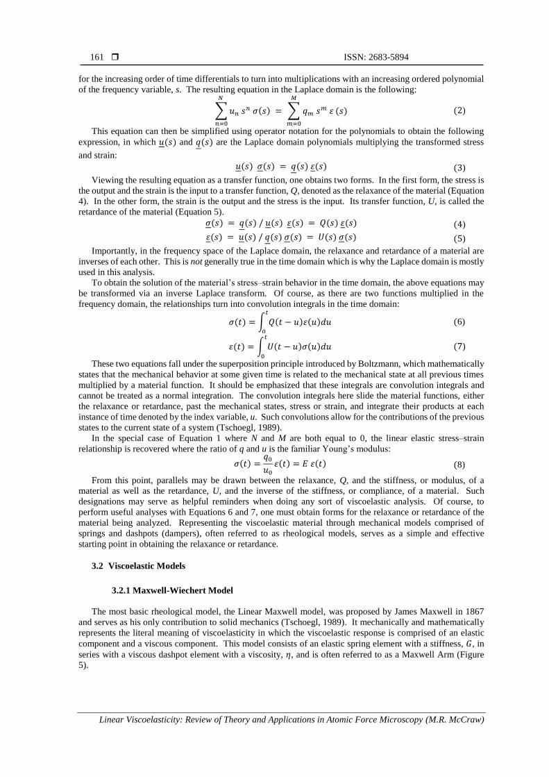
for the increasing order of time differentials to turn into multiplications with an increasing ordered polynomial

of the frequency variable, s. The resulting equation in the Laplace domain is the following:

∑ 𝑢𝑛 𝑠𝑛 𝜎(𝑠)

𝑁

𝑛=0

= ∑ 𝑞𝑚 𝑠𝑚 휀

𝑀

𝑚=0

(𝑠) (2)

This equation can then be simplified using operator notation for the polynomials to obtain the following

expression, in which 𝑢(𝑠) and 𝑞(𝑠) are the Laplace domain polynomials multiplying the transformed stress

and strain:

𝑢(𝑠) 𝜎(𝑠) = 𝑞(𝑠) 휀(𝑠) (3)

Viewing the resulting equation as a transfer function, one obtains two forms. In the first form, the stress is

the output and the strain is the input to a transfer function, Q, denoted as the relaxance of the material (Equation

4). In the other form, the strain is the output and the stress is the input. Its transfer function, U, is called the

retardance of the material (Equation 5).

𝜎(𝑠) = 𝑞(𝑠) / 𝑢(𝑠) 휀(𝑠) = 𝑄(𝑠) 휀(𝑠) (4)

휀(𝑠) = 𝑢(𝑠) / 𝑞(𝑠) 𝜎(𝑠) = 𝑈(𝑠) 𝜎(𝑠) (5)

Importantly, in the frequency space of the Laplace domain, the relaxance and retardance of a material are

inverses of each other. This is not generally true in the time domain which is why the Laplace domain is mostly

used in this analysis.

To obtain the solution of the material’s stress–strain behavior in the time domain, the above equations may

be transformed via an inverse Laplace transform. Of course, as there are two functions multiplied in the

frequency domain, the relationships turn into convolution integrals in the time domain:

𝜎(𝑡) = ∫ 𝑄(𝑡 − 𝑢)휀(𝑢)𝑑𝑢

𝑡

0

(6)

휀(𝑡) = ∫ 𝑈(𝑡 − 𝑢)𝜎(𝑢)𝑑𝑢

𝑡

0

(7)

These two equations fall under the superposition principle introduced by Boltzmann, which mathematically

states that the mechanical behavior at some given time is related to the mechanical state at all previous times

multiplied by a material function. It should be emphasized that these integrals are convolution integrals and

cannot be treated as a normal integration. The convolution integrals here slide the material functions, either

the relaxance or retardance, past the mechanical states, stress or strain, and integrate their products at each

instance of time denoted by the index variable, u. Such convolutions allow for the contributions of the previous

states to the current state of a system (Tschoegl, 1989).

In the special case of Equation 1 where N and M are both equal to 0, the linear elastic stress–strain

relationship is recovered where the ratio of q and u is the familiar Young’s modulus:

𝜎(𝑡) =𝑞0

𝑢0

휀(𝑡) = 𝐸 휀(𝑡) (8)

From this point, parallels may be drawn between the relaxance, Q, and the stiffness, or modulus, of a

material as well as the retardance, U, and the inverse of the stiffness, or compliance, of a material. Such

designations may serve as helpful reminders when doing any sort of viscoelastic analysis. Of course, to

perform useful analyses with Equations 6 and 7, one must obtain forms for the relaxance or retardance of the

material being analyzed. Representing the viscoelastic material through mechanical models comprised of

springs and dashpots (dampers), often referred to as rheological models, serves as a simple and effective

starting point in obtaining the relaxance or retardance.

3.2 Viscoelastic Models

3.2.1 Maxwell-Wiechert Model

The most basic rheological model, the Linear Maxwell model, was proposed by James Maxwell in 1867

and serves as his only contribution to solid mechanics (Tschoegl, 1989). It mechanically and mathematically

represents the literal meaning of viscoelasticity in which the viscoelastic response is comprised of an elastic

component and a viscous component. This model consists of an elastic spring element with a stiffness, 𝐺, in

series with a viscous dashpot element with a viscosity, 𝜂, and is often referred to as a Maxwell Arm (Figure

5).



Figure 5. Linear Maxwell Model or ‘Maxwell Arm’

While elementary, the Maxwell model allows for the physical recreation of steady-state flow and stress

relaxation (López-Guerra and Solares, 2014). For instance, when a step strain is initially applied to the model,

the damper resists motion proportional to the strain rate – an impulse occurring at the onset of strain. Due to

the impulse in force, all the applied strain is accommodated within the spring element which stores an internal

stress. After this instant, the damper yields which allows the compressed spring to release its stored energy,

thus relaxing the internal stress of the material. Additionally, if the strain is continuously applied, the material

will continuously and permanently deform, thus replicating steady state flow. By combining many Maxwell

arms in parallel with a single spring, 𝐺𝑒 , one obtains the Maxwell-Wiechert model. A general schematic of the

Maxwell-Wiechert model is provided in Figure 6.

Figure 6. Maxwell-Wiechert Model

The Maxwell-Wiechert model is capable of recreating the same physics as the Linear Maxwell model with

the addition of allowing for a mode of deformation recovery through the inclusion of the lone spring, 𝐺𝑒, which

may often be referred to as the elastic arm, restoring arm, or equilibrium modulus. Further, the addition of

multiple arms allows for the inclusion of multiple modes of stress relaxation occurring at different timescales,

each of which is related to the viscosity of the dashpot and the stiffness of the spring in each arm. If a Maxwell-

Wiechert model is constructed with a single Maxwell arm and the elastic spring, the resulting model is generally

referred to as a Standard Linear Solid (SLS) model (Findley et al., 1989). By removing the elastic arm from a

multi-arm Maxwell-Wiechert model, one obtains the Burger’s model, which is capable of modeling steady

state flow with the sacrifice of the recovery behavior (Findley et al., 1989). The elastic arm, 𝐺𝑒, is thus denoted

in brackets to indicate its optionality; if included, the model will recover, if not, the model will flow. The

mathematical details of such behaviors will be outlined in the following section.

To derive the behavior of the Maxwell-Wiechert model, it is convenient to begin with the behavior of a

single Maxwell arm (López-Guerra and Solares, 2014; Uluutku et al., 2021). The stress–strain relationship of

the elastic spring element and viscous dashpot element can be written as Equation 9 and 10, respectively:

𝜎 = 𝐺𝜖 (9)

𝜎 = 𝜂

𝑑𝜖

𝑑𝑡 (10)

163 ISSN: 2683-5894


When these two elements are connected in series, such as they are in a Maxwell arm, they will experience

the same amount of stress as expressed in Equation 11. Conversely, the total strain of the Maxwell arm is the

summation of the strains within the individual elements, as seen in Equation 12.

𝜎 = 𝜎𝑠 = 𝜎𝑑 (11)

𝜖 = 𝜖𝑠 + 𝜖𝑑 (12)

By substituting the stress–strain relationships for a spring (Equation 9) and a dashpot (Equation 10) into

the time derivative of Equation 12, the behavior of a single Maxwell arm can be written as the differential

equation provided in Equation 13. A simplification can be made by introducing a new parameter seen in

Equation 14. This parameter, referred to as a relaxation time, is defined as the ratio of the viscosity of the arm

dashpot and the stiffness of the arm spring. As such, it is a parameter that is specific to the Maxwell arm that

contains its spring and dashpot.

𝑑𝜖

𝑑𝑡=

𝑑𝜖𝑠

𝑑𝑡+

𝑑𝜖𝑑

𝑑𝑡=

1

𝐺

𝑑𝜎

𝑑𝑡+

𝜎

𝜂 (13)

𝜏 =𝜂

𝐺 (14)

By substituting the relaxation time of the Maxwell arm into its governing differential equation, Equation

15 is obtained. Like was done in Equations 1 and 2, the Laplace domain representation of the differential

stress–strain relationship may provide for more convenient solutions (Equation 16).

𝑑𝜖

𝑑𝑡=

1

𝐺

𝑑𝜎

𝑑𝑡+

𝜎

𝐺𝜏 (15)

𝜖𝑠 =

𝜎𝑠

𝐺+

𝜎

𝐺𝜏= 𝜎(

𝑠

𝐺+

1

𝐺𝜏)

(16)

By rearranging Equation 16 into a transfer function, one obtains the relaxance of the single Maxwell arm

as seen in Equation 17. Using this transfer function, which relates the stress and strain of an individual arm,

one can analyze the behavior of a Maxwell-Weichert model with an arbitrary number of arms, N. Given that

the total stress on the model should be equal to the sum of the stresses in each arm, the relaxance of each arm,

𝑄𝑖 , can be introduced to determine the stress–strain relationship (Equation 18). Further, given that the strain

on each arm is equal to the total strain of the model, the strain may be factored out of the sum and the relaxance

of the entire model may be obtained (Equation 19). The elastic arm spring, 𝐺𝑒, is included in the equation

through addition since it is in parallel with the remaining arms.

𝑄(𝑠) =

𝜎

𝜖= (

𝐺𝜏𝑠

𝜏𝑠 + 1) (17)

𝜎(𝑠) = ∑ 𝜎𝑖(𝑠)

𝑁

𝑖

= ∑ 𝜖𝑖(𝑠)𝑄𝑖

𝑁

𝑖

= 𝜖(𝑠) ∑ 𝑄𝑖

𝑁

𝑖

(18)

𝑄(𝑠) =

𝜎

𝜖 = ∑ 𝑄𝑖

𝑁

𝑖

= {𝐺𝑒} + ∑𝐺𝑖𝜏𝑖𝑠

1 + 𝜏𝑖 𝑠

𝑁

𝑖

(19)

An additional simplification can be made by substituting the sum of the stiffnesses of the springs in the

optional elastic arm and the remaining arms as in Equation 20.

𝐺𝑔 = {𝐺𝑒} + ∑ 𝐺𝑖

𝑁

𝑖

(20)

This new term, 𝐺𝑔, is the glassy modulus which represents the response of the Maxwell-Wiechert material

at infinitesimally short stressing times. Conversely, the elastic arm stiffness, 𝐺𝑒, or the equilibrium modulus,

represents the response of the material at infinitely long times. Equation 19 may then be simplified to Equation

21 in terms of the glassy modulus:

𝑄(𝑠) = 𝐺𝑔 − ∑𝐺𝑖

1 + 𝜏𝑖 𝑠

𝑁

𝑖

(21)

To analytically determine the stress response of a Maxwell-Wiechert material to common strain inputs, all

that is necessary is to multiply the Laplace domain representation of the desired input with the relaxance

transfer function for the Maxwell-Wiechert material, and then to take the inverse Laplace transformation of the

product.



3.2.1.1 Response to a Unit Impulse Strain

To replicate the response of a very rapid, impulse-like, indentation, a Dirac delta function may be used as

a strain input. Given that the unit impulse, or the Dirac delta function of unit coefficient, is simply

multiplication with unity in the Laplace domain, the response of a Maxwell model to an impulse strain may be

found by taking the inverse Laplace transform of the relaxance of the Maxwell model (Equation 22), giving

the result of Equation 23:

𝑄(𝑠) = 𝐺𝑒 + ∑𝐺𝑖𝜏𝑖𝑠

1 + 𝜏𝑖 𝑠=

𝑁

𝑖

𝐺𝑔 − ∑𝐺𝑖

1 + 𝜏𝑖 𝑠

𝑁

𝑖

(22)

𝑄𝑖𝑚𝑝𝑢𝑙𝑠𝑒(𝑡) = 𝐺𝑔𝛿(𝑡) − ∑𝐺𝑖

𝜏𝑖

𝑒−

𝑡𝜏𝑖

𝑁

𝑖

= (𝐺𝑒 + ∑ 𝐺𝑖

𝑁

𝑖

) 𝛿(𝑡) − ∑𝐺𝑖

𝜏𝑖

𝑒−

𝑡𝜏𝑖

𝑁

𝑖

(23)

The resulting equation is also termed the relaxance (in this case in the time domain), 𝑄(𝑡), and takes the

shape of an impulse which occurs at the onset of strain, followed by a series of negative, time decaying

exponentials. A plot of the response for an arbitrary, 2-arm Maxwell-Wiechert model is included in Table 1.

As can be seen, when the material exhibits steady state fluidity (mathematically, meaning that the equilibrium

modulus is zero), the exclusion of the elastic arm results in the weakening of the stress response of the model,

which is as expected from a more fluidic material. This function has a peculiar shape as a result of the Dirac

delta function and the negative exponentials; however, this function is the result of a non-physical strain

excitation and is primarily used for calculating the stress with Equation 6, when convolved with a strain

function.

3.2.1.2 Response to a Unit Step Strain

Replicating the procedure from above, a step input can be applied to the Laplace domain form of the transfer

function via multiplication with the Laplace domain representation of the step input, 1

𝑠:

𝐺𝑠𝑡𝑒𝑝(𝑠) =1

𝑠𝑄(𝑠) =

𝐺𝑒

𝑠+ ∑

𝐺𝑖𝜏𝑖

1 + 𝜏𝑖 𝑠=

𝑁

𝑖

=𝐺𝑔

𝑠− ∑

𝐺𝑖

𝑠 + 𝜏𝑖 𝑠2

𝑁

𝑖

(24)

The result of taking the inverse Laplace transformation of this expression gives the time domain response

of a Maxwell-Wiechert material to a step input, which is referred to as the relaxation, G:

𝐺𝑠𝑡𝑒𝑝(𝑡) = 𝐺𝑒 + ∑ 𝐺𝑖𝑒−

𝑡𝜏𝑖

𝑁

𝑖

= 𝐺𝑔 − ∑ 𝐺𝑖 (1 − 𝑒−

𝑡𝜏𝑖

𝑁

𝑖

) (25)

At the onset of strain, corresponding to t equal to zero, this expression indicates that the effective relaxation

of the material is the stiffer glassy modulus, 𝐺𝑔. At the instant of a specified relaxation time, 𝜏𝑖, the stress in

arm i will have decayed to 1

𝑒 of its original value, where e is the base of the natural logarithm. After sufficient

time, the material will relax to an effective relaxation equal to the weaker equilibrium modulus, 𝐺𝑒. However,

when the model exhibits steady state flow, the material will continue to creep until it fully relaxes under the

subjected strain. This equation may also be interpreted as the time integral of the unit impulse response.

3.2.1.3 Response to a Unit Ramp Strain

In an analogous manner as we proceeded above, the stress response of the model due to a unit ramp strain

input is obtained by multiplying the relaxance by 1

𝑠2 or by integrating the unit step response in time, giving the

result of Equation 26. If the model exhibits steady state fluidity, the response settles at a constant stress equal

to the sum of the products of the stiffness and the time constant of each arm. Otherwise, when the elastic term

is included, the stress will continue increasing at a rate proportional to the equilibrium modulus.

𝐺𝑟𝑎𝑚𝑝(𝑠) =1

𝑠2𝑄(𝑠) =

𝐺𝑔

𝑠2− ∑

𝐺𝑖

𝑠2 + 𝜏𝑖 𝑠3

𝑁

𝑖

(26)

𝐺𝑟𝑎𝑚𝑝(𝑡) = 𝐺𝑒𝑡 + ∑ 𝐺𝑖𝜏𝑛

𝑁

𝑖

(1 − 𝑒−

𝑡𝜏𝑖) = 𝐺𝑔𝑡 − ∑ 𝐺𝑖 (𝑡 − 𝜏𝑛 (1 − 𝑒

−𝑡𝜏𝑖))

𝑁

𝑖

(27)

165 ISSN: 2683-5894


Table 1. Maxwell-Weichert Model Standard Inputs and Time Domain Responses

Strain

Input Time Domain Response

Time Domain Response

w/ Steady State Fluidity Response Plot

Impulse 𝐺𝑔𝛿(𝑡) − ∑𝐺𝑖

𝜏𝑖

𝑒−

𝑡𝜏𝑖

𝑁

𝑖

∑ 𝐺𝑖

𝑁

𝑖

(𝛿(𝑡) −𝑒

− 𝑡𝜏𝑖

𝜏𝑖

)

Step 𝐺𝑒 + ∑ 𝐺𝑖𝑒−

𝑡𝜏𝑖

𝑁

𝑖

∑ 𝐺𝑖𝑒−

𝑡𝜏𝑖

𝑁

𝑖

Ramp 𝐺𝑒𝑡 + ∑ 𝐺𝑖𝜏𝑛

𝑁

𝑖

(1 − 𝑒−

𝑡𝜏𝑖) ∑ 𝐺𝑖𝜏𝑛

𝑁

𝑖

(1 − 𝑒−

𝑡𝜏𝑖)

3.2.1.4 Response to Harmonic Strains

When the Maxwell-Wiechert material is strained harmonically, the system can be analyzed in the Fourier

domain by substituting 𝑖𝜔 for the Laplace domain variable, 𝑠, as seen in Equation 28 below. The real and the

imaginary parts of the harmonic relaxance may be separated in the form shown in Equation 29.

𝑄(𝜔) = 𝐺𝑔 − ∑𝐺𝑖

1 + 𝑖𝜏𝑖𝜔

𝑁

𝑖

(28)

𝑄(𝜔) = 𝑄′(𝜔) + 𝑖𝑄′′(𝜔) (29)

The separated components of the relaxance are referred to as the storage modulus, 𝑄′, and loss modulus,

𝑄′′, respectively. As the names might suggest, these quantities determine how much energy storage and energy

dissipation a material displays at steady state at a given frequency; their exact forms are provided in Table 2

below (Tschoegl, 1989).

As the storage and loss moduli define a vector in the complex plane, the phase, or angle, of this vector may

be calculated through the inverse tangent of the ratio of the loss and storage moduli, as shown in Equation 30.

This quantity is referred to as the loss angle and the tangent of the loss angle is referred to as the loss tangent,

which can be seen in Equation 31 (Tschoegl, 1989).



𝜃(𝜔) = 𝑡𝑎𝑛−1

𝑄′′(𝜔)

𝑄′(𝜔) (30)

𝑡𝑎𝑛 𝜃(𝜔) =

𝑄′′(𝜔)

𝑄′(𝜔) (31)

The magnitude of the loss angle depends on the relative energy loss and storage of the material; typically,

the storage modulus increases with frequency as the molecules have less time to respond with slip-based

mechanisms and thus, can only respond through bond stretching (i.e., elastically). Further, the loss modulus

of a Maxwell-Wiechert material has distribution-like peaks whose centers correspond to the inverse of the

relaxation times of each arm. With multiple arms and multiple different relaxation times, the corresponding

loss modulus would have a number of identifiable peaks. Additionally, the larger the loss tangent, or the closer

the loss angle is to 90°, indicates that the material displays increasingly viscous behavior. Conversely, the

smaller the loss tangent, or the closer the loss angle is to 0°, indicates that the material displays increasingly

elastic behavior. For mostly elastic materials such as ceramics or metals, the loss tangent is typically around

0.001, and it is close to unity for highly dissipative materials, such as elastomers and biological materials

(Ferry, 1980; Proksch et al., 2016). As could be anticipated, when the material exhibits steady state flow, its

ability to store energy is greatly diminished as the material yields continuously.

3.2.2 Kelvin-Voigt Model

In practical cases, it may be more convenient to use stress as the input of the material model as opposed to

strain. In this case, an analogous model to the Maxwell-Wiechert model may be constructed, but which allows

for a more convenient strain input analysis. In the Voigt model, an elastic spring and a viscous dashpot are

combined in parallel rather than in series, as seen in Figure 7. The resulting combination allows for the

modelling of creep and recovery, but is incapable of replicating steady state flow and stress relaxation (Findley

et al., 1989; Tschoegl, 1989). When subjected to a step input of stress, the dashpot will slow down the strain

response of the system. The dashpot stress weakens as time progresses, until the spring entirely bears the stress

input – at this final stage, the material has creeped to a resting point. Once the applied stress is released, the

energy stored in the spring will slowly restore the material to its original position. Like the linear Maxwell

model, the capabilities of the Voigt model may be enhanced by including additional Voigt ‘units’ in series with

an elastic spring. The resulting Kelvin-Voigt model can be seen in Figure 8.

During the application of a stress input to the Kelvin-Voigt model, the stress stored in the lone elastic spring

may be relaxed through the deformations of the Voigt units in the model. Thus, the Kelvin-Voigt model, like

the Maxwell-Weichert model, is capable of modeling creep, recovery, stress relaxation, and steady state flow;

although the latter is only possible when an optional dashpot is added in series with the model as seen in the

bracketed dashpot denoted as 𝜑f in Figure 8.

Similar analytical exercises can be carried out for the Kelvin-Voigt model as for the Maxwell-Wiechert

model to determine the response of a Kelvin-Voigt material to common stress inputs. Because of the

construction of the model, each Voigt unit experiences the same applied stress but responds with different

internal strains. However, inside of a single Voigt unit, the strain of the spring and the dashpot element are

equal, meanwhile they will experience different stresses. The total stress of a single Voigt unit can thus be

written as the relation in Equation 32:

𝜎 = 𝜎𝑠𝑝𝑟𝑖𝑛𝑔 + 𝜎𝑑𝑎𝑠ℎ𝑝𝑜𝑡 (32)

From here, the stress–strain relationship of a single Voigt unit may be written by substituting the individual

stress–strain equations for the spring and the dashpot, as seen in Equation 33. Again, recasting this equation

into the Laplace domain provides for a more convenient manipulation as seen in Equation 34.

𝜎(𝑡) = 𝐺휀(𝑡) + 𝜂휀′(𝑡) (33)

𝜎(𝑠) = 𝐺휀(𝑠) + 𝜂𝑠휀(𝑠) = 휀(𝑠) × (𝐺 + 𝜂𝑠) (34)

Factoring out the strain term yields the more concise Equation 35:

휀(𝑠) = 𝜎(𝑠)

1

(𝐺 + 𝜂𝑠) (35)

167 ISSN: 2683-5894


Table 2. Maxwell-Weichert Model Harmonic Quantities

Harmonic

Quantity Form Plot

Storage

Modulus {𝐺𝑒} + ∑ 𝐺𝑖(1 −

1

1 + 𝜏𝑖2𝜔2

)

𝑁

𝑖

Loss

Modulus ∑

𝐺𝑖𝜔𝜏𝑖

1 + 𝜏𝑖2𝜔2

𝑁

𝑖

Loss

Tangent

Q′′(ω)

Q′(ω)

Figure 7. Linear Voigt Model



Figure 8. Kelvin-Voigt Model

With such a formulation, it is customary to exchange the inverse of the spring stiffness, G, for a compliance,

𝐽, and the inverse of the dashpot viscosity, 𝜂, for a fluidity, 𝜑, where the names are self-explanatory. The

mathematical relationships are presented in Equation 36. Thus, the stress–strain relationship of the single Voigt

unit may be rewritten in terms of the compliance and fluidity as seen in Equation 37.

𝐽 =

1

𝐺, 𝜑 =

1

𝜂 (36)

휀(𝑠) = 𝜎(𝑠)

1

(1𝐽

+1𝜑

𝑠)= 𝜎(𝑠)

𝐽

(1 +𝐽𝜑

𝑠) (37)

Similar to the relaxation time of the Maxwell-Wiechert model, a retardation time, 𝜏, may be introduced for

each Voigt unit, which is defined as the ratio of the compliance of the spring and the fluidity of the dashpot

within a given Voigt unit, as defined in Equation 38. Substituting the retardation time into Equation 37 yields

the simplified relationship provided in Equation 39.

𝜏 =

𝐽

𝜑 (38)

휀(𝑠) = 𝜎(𝑠)

𝐽

(1 + 𝜏𝑠) (39)

As for the Maxwell-Wiechert model, the stress–strain relationship may be rearranged into a transfer

function with stress as the input and strain as the output. This resulting transfer function, given in Equation

40, is referred to as the retardance, U, of a single Voigt unit. As the retardance is analogous to the inverse of

the stiffness, the total retardance of a Kelvin-Voigt model may be obtained by directly summing the retardance

of each Voigt unit in the model as in the sum presented in Equation 41.

𝑈𝑢𝑛𝑖𝑡(𝑠) =

휀(𝑠)

𝜎(𝑠)= 𝜎(𝑠)

𝐽

(1 + 𝜏𝑠) (40)

휀(𝑠) = 𝜎𝑖(𝑠) ∑ 𝑈𝑖

𝑁

𝑖

(41)

Here, 𝑈𝑖 represents the retardance of the ith of N Voigt units in a Kelvin-Voigt material. Substituting the

equation for the retardance of each Voigt unit as well as the compliance of the lone elastic spring, 𝐽𝑔, and

fluidity of the optional steady-state fluidity dashpot, 𝜑, the exact form of the retardance of a Kelvin-Voigt

material is obtained in Equation 42. As for the Maxwell-Wiechert model, a substitution can be made as seen

in Equation 43 where the equilibrium compliance, 𝐽𝑒, is written in terms of the glassy compliance, 𝐽𝑔, and the

compliances of the springs in each arm, 𝐽𝑖.

𝑈(𝑠) =휀(𝑠)

𝜎(𝑠) = ∑ 𝑈𝑖

𝑁

𝑖

= 𝐽𝑔 + ∑𝐽𝑖

1 + 𝜏𝑖 𝑠

𝑁

𝑖

+ {𝜑

𝑠} (42)

169 ISSN: 2683-5894


𝐽𝑒 = 𝐽𝑔 + ∑ 𝐽𝑖

𝑁

𝑖

(43)

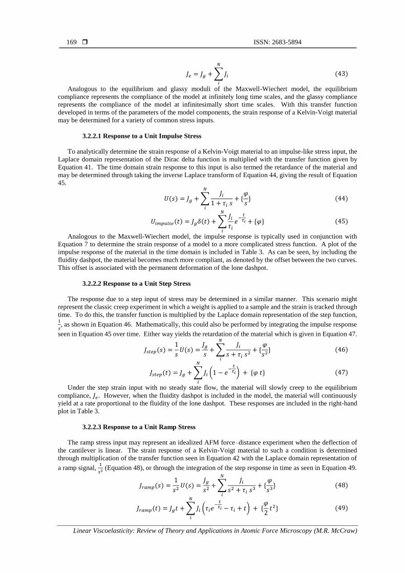
Analogous to the equilibrium and glassy moduli of the Maxwell-Wiechert model, the equilibrium

compliance represents the compliance of the model at infinitely long time scales, and the glassy compliance

represents the compliance of the model at infinitesimally short time scales. With this transfer function

developed in terms of the parameters of the model components, the strain response of a Kelvin-Voigt material

may be determined for a variety of common stress inputs.

3.2.2.1 Response to a Unit Impulse Stress

To analytically determine the strain response of a Kelvin-Voigt material to an impulse-like stress input, the

Laplace domain representation of the Dirac delta function is multiplied with the transfer function given by

Equation 41. The time domain strain response to this input is also termed the retardance of the material and

may be determined through taking the inverse Laplace transform of Equation 44, giving the result of Equation

45.

𝑈(𝑠) = 𝐽𝑔 + ∑𝐽𝑖

1 + 𝜏𝑖 𝑠

𝑁

𝑖

+ {𝜑

𝑠} (44)

𝑈𝑖𝑚𝑝𝑢𝑙𝑠𝑒(𝑡) = 𝐽𝑔𝛿(𝑡) + ∑𝐽𝑖

𝜏𝑖

𝑒−

𝑡𝜏𝑖

𝑁

𝑖

+ {𝜑} (45)

Analogous to the Maxwell-Wiechert model, the impulse response is typically used in conjunction with

Equation 7 to determine the strain response of a model to a more complicated stress function. A plot of the

impulse response of the material in the time domain is included in Table 3. As can be seen, by including the

fluidity dashpot, the material becomes much more compliant, as denoted by the offset between the two curves.

This offset is associated with the permanent deformation of the lone dashpot.

3.2.2.2 Response to a Unit Step Stress

The response due to a step input of stress may be determined in a similar manner. This scenario might

represent the classic creep experiment in which a weight is applied to a sample and the strain is tracked through

time. To do this, the transfer function is multiplied by the Laplace domain representation of the step function, 1

𝑠, as shown in Equation 46. Mathematically, this could also be performed by integrating the impulse response

seen in Equation 45 over time. Either way yields the retardation of the material which is given in Equation 47.

𝐽𝑠𝑡𝑒𝑝(𝑠) =1

𝑠𝑈(𝑠) =

𝐽𝑔

𝑠+ ∑

𝐽𝑖

𝑠 + 𝜏𝑖 𝑠2

𝑁

𝑖

+ {𝜑

𝑠2} (46)

𝐽𝑠𝑡𝑒𝑝(𝑡) = 𝐽𝑔 + ∑ 𝐽𝑖 (1 − 𝑒−

𝑡𝜏𝑖)

𝑁

𝑖

+ {𝜑 𝑡} (47)

Under the step strain input with no steady state flow, the material will slowly creep to the equilibrium

compliance, 𝐽𝑒. However, when the fluidity dashpot is included in the model, the material will continuously

yield at a rate proportional to the fluidity of the lone dashpot. These responses are included in the right-hand

plot in Table 3.

3.2.2.3 Response to a Unit Ramp Stress

The ramp stress input may represent an idealized AFM force–distance experiment when the deflection of

the cantilever is linear. The strain response of a Kelvin-Voigt material to such a condition is determined

through multiplication of the transfer function seen in Equation 42 with the Laplace domain representation of

a ramp signal, 1

𝑠2 (Equation 48), or through the integration of the step response in time as seen in Equation 49.

𝐽𝑟𝑎𝑚𝑝(𝑠) =1

𝑠2𝑈(𝑠) =

𝐽𝑔

𝑠2+ ∑

𝐽𝑖

𝑠2 + 𝜏𝑖 𝑠3

𝑁

𝑖

+ {𝜑

𝑠3} (48)

𝐽𝑟𝑎𝑚𝑝(𝑡) = 𝐽𝑔𝑡 + ∑ 𝐽𝑖 (𝜏𝑖𝑒−

𝑡𝜏𝑖 − 𝜏𝑖 + 𝑡)

𝑁

𝑖

+ {𝜑

2𝑡2} (49)



As seen in the response plot in Table 3, the Kelvin-Voigt material will continuously yield under the

consistently increasing ramp stress. When the material exhibits steady state fluidity, the material simply yields

at a higher rate.

Table 3. Kelvin-Voigt Model Standard Inputs and Time Domain Responses

Stress

Input Time Domain Response

Time Domain Response w/

Steady State Fluidity Response Plot

Impulse Jgδ(t) + ∑Ji

τi

e−

tτi

N

i

Jgδ(t) + ∑Ji

τi

e−

tτi

N

i

+ φ

Step Jg + ∑ Ji (1 − e−

tτi)

N

i

Jg + ∑ Ji (1 − e−

tτi)

N

i

+ φ t

Ramp Jgt + ∑ Ji (τie−

tτi − τi + t)

N

i

Jgt + ∑ Ji (τie

−t

τi − τi + t)

N

i

+ φ

2t2

3.2.2.4 Response to Harmonic Stresses

The response of a Kelvin-Voigt material under steady-state harmonically oscillating stresses can be easily

determined by evaluating the transfer function when the Laplace domain variable, 𝑠, is equal to 𝑖𝜔, as done

with the Maxwell-Wiechert model. This Fourier domain representation of the retardance, seen in Equation 50,

can then be separated into real and imaginary components, which yields the storage compliance and loss

compliance, respectively, as given in Equation 51.

𝑈(𝜔) = 𝐽𝑔 + ∑𝐽𝑖

1 + 𝑖𝜏𝑖𝜔

𝑁

𝑖

− {𝑖𝜑

𝜔} (50)

𝑈(𝜔) = 𝑈′(𝜔) − 𝑖𝑈′′(𝜔) (51)

171 ISSN: 2683-5894


The exact forms of the storage and loss compliance can be found in Table 4. As was claimed in the

Maxwell-Wiechert model derivation, the storage compliance is a measure of the energy stored in the material,

while the loss compliance is a measure of the energy that is lost in the material. The loss compliance for a

Maxwell-Wiechert model displays distribution-like peaks with their centers located at the inverse of the

retardation time, 1

𝜏, of each unit. Additionally, the angle between the storage and loss compliance is again

denoted as the loss angle with the tangent of the loss angle being referred to as the loss tangent, given in

Equations 52 and 53. These two quantities determine the degree to which the strain response is elastic or

viscous, corresponding to small and large loss tangents, respectively. Unsurprisingly, when the material

exhibits steady state fluidity, the loss compliance always increases by an offset that is proportional to the

fluidity of the lone dashpot.

𝜃(𝜔) = 𝑡𝑎𝑛−1

𝑈′′(𝜔)

𝑈′(𝜔) (52)

𝑡𝑎𝑛 𝜃(𝜔) =

𝑈′′(𝜔)

𝑈′(𝜔) (53)

3.2.3 Power Law Rheology

While the Maxwell-Wiechert and Kelvin-Voigt material models are capable of recreating the many

complex phenomena seen in linear viscoelastic solid mechanics, the number of arms may seem to be an

arbitrary constant which could be justified through a number of ways. In some cases, it may be preferred to

determine the same model behaviors when the there are an infinite number of arms in each model. In this case,

an integration may be performed over the relaxation or retardation time variables, while treating the stiffness

or compliance of the springs as a spectra, as described in Equation 54 (Efremov et al., 2020; Findley et al.,

1989; Tschoegl, 1989).

𝜖𝑠𝑡𝑒𝑝 = 𝜎𝑠𝑡𝑒𝑝 [𝐽𝑔 + ∑ 𝐽𝑛(1 − 𝑒−

𝑡𝜏𝑛)

∞

𝑛=0

] ≅ 𝜎0 [𝐽𝑔 + ∫ 𝐽(𝜏)(1 − 𝑒−𝑡𝜏)

∞

0

𝑑𝜏] (54)

Without knowing the shape of the relaxation or retardation spectra, an assumption of the time dependent

material behavior is necessary to determine the shape of the relevant spectra of a material. In this case, it has

been empirically observed that the stress–strain behavior of many materials follows a power law shape in their

creep relaxation and retardation behavior, as per Equation 55 (Findley et al., 1989; Tschoegl, 1989). In this

equation, the step response is modelled by a constant offset followed by a time dependent transient response

dictated by the arbitrary exponent, n, which is a material parameter that is independent of temperature and

generally less than 1.

𝜖𝑠𝑡𝑒𝑝(𝑡) = 𝜖 + 𝜖+𝑡𝑛, 𝜎𝑠𝑡𝑒𝑝(𝑡) = 𝜎 + 𝜎+𝑡𝑛 (55)

By setting the integral relationship in Equation 54 equal to the power law relationship in Equation 55, the

retardation spectra may be determined. Of course, the integral in Equation 54 converges conditional to the

selection of the retardation spectra. Specifically, when 𝐽(𝜏) is chosen to be equal to that of Equation 56, the

empirically observed Power Law Rheology (PLR) behaviors seen in Equation 55 may be obtained.

𝐽(𝜏) =

𝑛𝑚𝜏𝑛−1

𝛤(1 − 𝑛) (56)

The storage and loss compliances of this model may be calculated by taking a Fourier transform of equation

56 and taking the derivative with respect to time (hence multiplying by iω in the Fourier domain) as seen in

Equations 57 and 58, in which k is an integer (Findley et al., 1989). Note that these relationships are only

obtained by taking the retardation spectra presented in Equation 56.

𝑈′(𝜔) = 𝐽𝑔 + 𝐽+𝛤(𝑛 + 1)𝜔−𝑛 𝑐𝑜𝑠(𝑛𝜋

2+ 2𝑘𝑛𝜋) (57)

𝑈′′(𝜔) = 𝐽+𝛤(𝑛 + 1)𝜔−𝑛 𝑠𝑖𝑛(𝑛𝜋

2+ 2𝑘𝑛𝜋) (58)

With different spectra, different power law stress–strain relationships or even non-power-law relationships

may be obtained (Tschoegl, 1989). Additionally, the derivation of such relationships could be equivalently

done for Maxwell-Wiechert models. Recently, the modified power law relaxation modulis in Equation 59

has gained popularity in the description of biological materials (Efremov et al., 2020). The modified power

law is desirable as it avoids the mathematical singularities of more basic power laws which occur at the onset

of strain (WILLIAMS, 1964). Additional power law relationships may be derived by replacing elements of

either the Maxwell or Voigt models with fractional viscoelastic elements whose stress behavior depends on a

fractional time derivative of the strain (Bonfanti et al., 2020).



𝐺𝑠𝑡𝑒𝑝 = 𝐺𝑔 (1 +

𝑡

𝜏0

)−𝑛

(59)

Table 4. Kelvin-Voigt Model Harmonic Quantities

Harmonic

Quantity Form Plot

Storage

Compliance Jg + ∑

Jn

1 + τn2ω2

n

Loss

Compliance ∑

Jnωτn

1 + τn2ω2

n

+ {φ

ω}

Loss

Tangent

U′′(ω)

U′(ω)

3.3 Utilizing Viscoelastic Models

Once a desired viscoelastic model has been selected to represent the behavior of a given material, the

material’s response to an arbitrary, time-dependent stress or strain can be calculated from the desired form of

the relaxance or retardance, as outlined above. As already stated, the relaxance or retardance can be convolved

with the arbitrary, time-dependent strain or stress as per the Boltzmann superposition principle stated in

Equations 6 and 7. In essence, this way of modeling the material response imposes the unit stress or strain

input on the material at every instant throughout its time-dependent stress or strain excitation. For instance,

when using the relaxance, or the stress response of a strain impulse, the resulting strain function is

mathematically constructed by a continuous set of strain impulses. Likewise, the resulting stress function is

173 ISSN: 2683-5894


constructed from a continuous set of stress responses from each strain impulse (Tschoegl, 1989). Thus, the

linear nature of linear viscoelasticity again becomes apparent. Although these mechanical descriptions can

recreate the complex stress–strain dynamics of viscoelastic materials, it is often experimentally inconvenient

to make calculations with the stress and strain of the material. This inconvenience becomes exceptionally

relevant in the case of the analysis of data obtained through an AFM experiment, where the strain calculation

may be ambiguous and the determination of the surface area used for calculating the stress becomes

exceedingly difficult to resolve. To extend the usefulness of the previously outlined theories, the stress–strain

relationship needs to be recast in consideration of the contact mechanics of typical AFM experiments.

4. Contact Mechanics

4.1 Hertzian Contact Models

The Hertzian Contact theory is the most commonly used contact model for elastic bodies in contact

(Johnson, 1982, 1985). The elastic contact between an AFM tip and the surface of a sample is commonly

modeled using a Hertzian contact model, in which the tip and the sample are modeled as a sphere, cone, or

circular flat punch interacting with a flat surface, depending on the type of AFM tip chosen for the experiment

(Eaton and West, 2010; Morris et al., 2009). The observables in the contact mechanical description of the

indentation of the tip into the surface are the force and indentation depth, rather than the stress and strain.

Additionally, considerations of the geometry of the tip are factored in through the radius of curvature (𝑟), angle

of separation (𝜃), and the radius of the circular face (𝑅) in the cases for a spherical, conical, and flat punch tips,

respectively (see Table 5). Further, the reduced elastic modulus of the sample is used to simplify the resulting

equations as expressed in Equation 60. The use of this reduced elastic modulus requires the assumption that

the material in the tip is significantly stiffer than the sample, which works well when measuring softer materials

with stiffer AFM tips. The resulting force–indentation relationships are provided in Table 5.

1

𝐸∗=

1 − 𝜈12

𝐸1

(60)

By using these forms of the Hertzian contact models for analyzing the mechanics of an elastic sample, it is

again required that the tip be significantly stiffer than the sample, the strains are small, the contact area is small

relative to the sample, the sample thickness is large enough compared to the indentation so as to be considered

infinite, and the contact region is free from friction effects (Eaton and West, 2010). In recent work, it has been

shown that in small samples, such as individual cells, the assumption of infinite sample thickness may introduce

large numerical errors when analyzing the mechanical properties of a sample (Garcia and Garcia, 2018).

4.2 Viscoelastic Contact Models

To extend the usefulness of the Hertzian contact models from elastic materials to viscoelastic

materials, one may start with the generalized form of the Hertzian pressure distribution as seen in Equation 61

in which, 𝑓(𝛽, 𝑡) is a function that describes the depth of indentation as a function of time and tip geometry

(Garcia et al., 2020). The constant 𝛼 represents a geometry dependent constant which scales the pressure–

indentation relationship and has been included as part of the equations in Table 5 and explicitly written in Table

6.

𝑝(𝑡) = 𝛼 𝐸 𝑓(𝛽, 𝑡) (61)

As was done when initially deriving the relaxance and retardance of the Maxwell-Wiechert and Kelvin-

Voigt models, the Laplace transform of the equation may be taken to result in more convenient manipulations

as seen in Equation 62.

𝑝(𝑠) = 𝛼 𝐸 𝑓(𝛽, 𝑠) (62)

The developers of the theory of viscoelastic contact, Lee and Radok, argue that the Young’s modulus, 𝐸,

of the material could be equivalently substituted by its viscoelastic analogue, the relaxance, 𝑄(𝑠), as seen in

between Equations 62 and 63 (Lee and Radok, 1960; Tschoegl, 1989). Integrating this pressure distribution

over the contact region yields an equivalent expression for the force as a function of the indentation, tip

geometry, and relaxance of the material as seen in Equation 64.

𝑝(𝑠) = 𝛼 𝑄(𝑠) 𝑓(𝛽, 𝑠) (63)

𝐹(𝑠) = 𝛼 𝑄(𝑠) 𝑓′(𝛽, 𝑠) (64)

Table 5. Elastic Hertzian Contact Models for Typical AFM Geometries



Tip Shape Contact Model System Diagram

Sphere 𝐹 =4

3𝐸∗√𝑟 ℎ3

Cone 𝐹 =2

𝜋𝐸∗

ℎ2

tan (𝜃)

Flat-Punch 𝐹 = 2 𝑅 𝐸∗ ℎ

From this point, the force equation may be equivalently reformulated to express the indentation as a function

of force, tip geometry, and the retardance of the material. By taking the inverse Laplace transformation of the

expression for force or indentation, the time domain solutions of the force–indentation relationships are

obtained (Lee and Radok, 1960; Tschoegl, 1989). Equations 65 and 66 display these relationships in which

the indentation, h, has been properly substituted:

𝐹(𝑡) = 𝛼 ∫ 𝑄𝑖𝑚𝑝𝑢𝑙𝑠𝑒(𝑡 − 𝑢) ℎ𝛽(𝑢) 𝑑𝑢

𝑡𝑓

0

(65)

ℎ𝛽(𝑡) =

1

𝛼 ∫ 𝑈𝑖𝑚𝑝𝑢𝑙𝑠𝑒(𝑡 − 𝑢) 𝐹(𝑢)𝑑𝑢

𝑡𝑓

0

(66)

The resulting viscoelastic contact models from Lee’s and Radok’s derivation require that the deformation

be small relative to the contact area and that the force monotonically increase (Garcia, 2020; Garcia et al.,

2020; Lee and Radok, 1960). The latter assumption has been investigated to extend the theory to include the

unloading regime and it has been shown that the error is small, especially in the case when the unloading is

relatively fast (Cheng and Cheng, 2005; Greenwood, 2010). More mathematically valid for the case of non-

monotonically increasing force is the Ting model provided in Equation 67. This model convolves the

relaxation (step response of a Maxwell-Wiechert material) and the derivative of the scaled indentation which

allows for the analysis of forces which increase and subsequently decrease after a single maximum (Garcia et

al., 2020; Ting, 1966, 1968). As a word of precaution, Equation 67 may provide inaccurate results when used

with experimental data with excessive noise due to the numerical derivative of the indentation.

𝐹(𝑡) = 𝛼 ∫ 𝐺𝑠𝑡𝑒𝑝(𝑡 − 𝑢)

𝑑 ℎ𝛽(𝑢)

𝑑𝑢 𝑑𝑢

𝑡𝑓

0

(67)

175 ISSN: 2683-5894


Table 6. Viscoelastic Contact Model Parameters for Typical AFM Geometries

The above equations are similar in form to the Boltzmann superposition integral in that they contain a

convolution between a material function, either the relaxance, retardance, or relaxation, and a material

observable, either the indentation or the force. It should be reiterated that this is not a normal integral operator,

and therefore treating it as such will not give correct results. In a computational scheme, numerical convolution

operations should be performed. Further, depending on the choice of equation, either the time domain form of

the material’s relaxance, 𝑄(𝑡), retardance, 𝑈(𝑡), or relaxation, 𝐸(𝑡) should be used in the convolution. While

a variety of forms of relaxances, relaxations, retardances, and retardations have been provided in Tables 1 and

3 as well as Equation 59, if one were to obtain alternate expressions for these material functions, the viscoelastic

contact mechanical descriptions presented in Table 6 may still be used in the same way.

5. Mapping AFM Experiments to Theory

One of the more useful applications of the contact mechanical descriptions is in the analysis of force–

distance curves obtained from AFM measurements. Such an analysis, often referred to as the “inversion” of a

force curve, enables AFM users to obtain the viscoelastic parameters which best describe the material being

studied, and is described in detail elsewhere (López-Guerra and Solares, 2017; Parvini et al., 2020). The

inversion involves fitting a contact mechanical model of the desired viscoelastic material model to the

experimentally obtained force distance curves (López-Guerra et al., 2017). Generally, fits are performed

Tip Shape 𝛼 𝛽 System Diagram

Sphere 4 √𝑟

3 (1 − 𝜐2)

3

2

Cone 2 tan (𝜃)

𝜋(1 − 𝜐2) 2

Flat-Punch 2 R

(1 − 𝜐2) 1



through the minimization of a specific objective function, such as the mean squared error or sum of squared

errors. An example of the sum of squared errors objective function for a Kelvin-Voigt material is given in

Equation 68 below. Here, the indentation, ℎ𝐴𝐹𝑀 , and force, 𝐹AFM, obtained from an AFM experiments are

used.

𝑆𝑆𝐸 = ∑(𝛼 ∫ 𝑈𝑖𝑚𝑝𝑢𝑙𝑠𝑒(𝑡 − 𝑢) 𝐹𝐴𝐹𝑀(𝑢)𝑑𝑢𝑡

0

− ℎ𝐴𝐹𝑀𝛽

(𝑡))2

𝑡𝑓

0

(68)

Of course, one could also perform a convolution of the retardance with the force curve to obtain a

‘prediction’ of the scaled, experimental indentation, ℎAFM𝛽

. The difference between this ‘predicted’ scaled

indentation and the actual scaled indentation is then summed to determine the total error for a given set of

Kelvin-Voigt material parameters such as N, 𝐽𝑔, 𝐽𝑖, and τi (López-Guerra et al., 2017). The large number of

degrees of freedom in this fit tends to make the process of fitting and obtaining a mechanically meaningful

parameter set very difficult. It is also difficult to interpret and determine which parameter sets are mechanically

meaningful. For this reason, it is common to use power law representations such as that in Equation 59 as they

tend to fit AFM data better in some cases (Efremov et al., 2020). Additional care should be taken when using

material functions that include Dirac delta functions such as those seen in the relaxance for the Maxwell-

Wiechert model and the retardance for the Kelvin-Voigt model. In these instances, the integrand of the

convolution should be simplified as much as possible with the intention of analytically evaluating any delta

functions that may be present. Such an example is given for the Maxwell-Wiechert step response in Equation

69.

𝐹(𝑡)

𝛼= ∫ (𝐺𝑔𝛿(𝑡 − 𝑢) − ∑

𝐺𝑖

𝜏𝑖

𝑒−

𝑡−𝑢𝜏𝑖

𝑁

𝑖

)ℎ𝛽(𝑢) 𝑑𝑢𝑡𝑓

0

=

= 𝐺𝑔ℎ𝛽(𝑡) − ∫ ∑𝐺𝑖

𝜏𝑖

𝑒−

𝑡−𝑢𝜏𝑖

𝑁

𝑖

ℎ𝛽(𝑢) 𝑑𝑢𝑡𝑓

0

(69)

Furthermore, numerical convolution schemes should be used to handle the convolution integrals rather than

normal numerical integration schemes – doing the latter would result in inaccuracies that may not obviously

manifest themselves. Lastly, one should always consider restricting any possible time constants of any material

models used to be above the experimental sampling frequency, as well as under the experiment duration.

Obtaining and citing any time constants, such as the relaxation time, that are outside of these bounds would be

an extrapolation of the experimental data rather than an observational quantity.

6. Model-Free Viscoelasticity

Recent developments have allowed the viscoelastic contact mechanics equations to be used without a

specific material model when analyzing experimental data (Uluutku et al., 2021). This approach requires the

use of a frequency domain technique like the Laplace or Fourier transforms used in analyzing the previously

discussed viscoelasticity models. By recasting the experimental data in a frequency domain, the relaxance,

relaxation, retardance, or retardation may be directly obtained. Of course, the storage and loss behaviors of a

material may be obtained through Fourier transformations of data from harmonic, steady-state experiments.

However, when used for a non-harmonic, and non-bounded functions such as those present in force–distance

experiments, Fourier techniques give faulty results and do not correspond the analytical theory (Aspden, 1991;

Uluutku et al., 2021). This mismatch can be said to be caused by the un-bounded nature of the signals and

finite bandwidth of the experiments. To avoid the limitations of discrete Fourier techniques, it has recently

been proposed to use the ‘discrete Laplace transform,’ known as the Z-Transform, to analyze experimental

data (Oppenheim and Schafer, 1975; Uluutku et al., 2021). By using the Z- and modified Fourier transforms,

one can directly access the storage and loss behaviors of a material. The Z-Transform of a discrete signal, f,

may be obtained through Equation 70:

𝑍{𝑓[𝑛]} = 𝐹(𝑧) = ∑ 𝑓[𝑛]𝑧−𝑛

𝑛

(70)

Using this ‘discrete Laplace transform’ the contact mechanics models presented in Equations 65, 66, and

67 may be transformed into a discrete form of Equation 64, as expressed in Equation 71.

𝑄(𝑧) =

1

𝛼

𝐹(𝑧)

𝑍{ℎ𝛽} (71)

177 ISSN: 2683-5894


This Laplace domain representation may be manipulated to directly obtain either the relaxance, relaxation,

retardance, or retardation for a given force curve, using the force, F, and the indentation, h, as input. The

discrete modified Fourier transform of the same signal, f, from Equation 70 may be determined by evaluating

the Z-Transform at 𝑧 = 𝑒𝛽𝑜𝑒𝑖𝜃 in the range of 𝜃 between 0 and 2𝜋, as in Equation 72. By performing this

discrete modified Fourier transformation to the contact mechanics models, the resulting relationship may be

manipulated like before to obtain Equation 73.

𝐹{𝑓[𝑛], 𝛽0} = 𝐹(𝑖𝜔, 𝛽0) = 𝐹𝐹𝑇(𝑓[𝑛]𝑒−𝛽0𝑛) (72)

𝑄(𝑖𝜔, 𝛽𝑜) =

1

𝛼

𝐹(𝑖𝜔, 𝛽𝑜)

𝐹{ℎ𝛽} (73)

Separating the real and imaginary components of the resulting material function yields the storage and loss

behaviors of the given material. It has been determined that when this discrete result is compared to that of a

Kelvin-Voigt and Maxwell-Wiechert models, the modified storage and loss behaviors have similar shapes to

the analytical models in terms of the locations of the characteristic times; however, the modified storage and

loss behaviors tend to be more spread across the frequency axis by a factor depending on the experimental

sampling and 𝛽0. This is discussed in detail elsewhere (Uluutku et al., 2021).

The power of such an approach may be better appreciated when compared to the results of the inversion of

force curves. By fitting the contact mechanics models to AFM data, a margin of error is incorporated into the

resulting viscoelastic parameters. Additionally, when using the Kelvin-Voigt or Maxwell-Wiechert models it

is often a difficult task to determine whether a set of parameters is mechanically meaningful or not. By using

the Z-Transform approach, the material function of a material is directly obtained without having to assume

that it follows the behavior of a specific model and without the use of a fitting algorithm (Uluutku et al., 2021).

Therefore, viscoelastic material behaviors may be very accurately obtained through the use of both Z- and

discrete modified Fourier transforms.

Acknowledgement: The paper is a product of the research performed within project CMMI-2019507,

supported by the U.S. National Science Foundation, whom the authors gratefully acknowledge.

References

Aspden, R.M. (1991). Aliasing effects in Fourier transforms of monotonically decaying functions and the

calculation of viscoelastic moduli by combining transforms over different time periods, Journal of

Physics D: Applied Physics, 24(6), 803–808.

Binnig, G., Quate, C.F. and Gerber, C. (1986). Atomic Force Microscope, Physical Review Letters, 56(9),

930–933.

Binnig, G. and Rohrer, H. (1983). Scanning tunneling microscopy, Surface Science, 126(1–3), 236–244.

Bonfanti, A., Kaplan, J.L., Charras, G. and Kabla, A. (2020). Fractional viscoelastic models for power-law

materials, Soft Matter, 16(26), 6002–6020.

Cheng, Y.-T. and Cheng, C.-M. (2005). Relationships between initial unloading slope, contact depth, and

mechanical properties for conical indentation in linear viscoelastic solids, Journal of Materials

Research, 20(4), 1046–1053.

Eaton, P. and West, P. (2010). Atomic Force Microscopy, Oxford University Press, available

at:https://doi.org/10.1093/acprof:oso/9780199570454.001.0001.

Efremov, Y.M., Okajima, T. and Raman, A. (2020). Measuring viscoelasticity of soft biological samples

using atomic force microscopy, Soft Matter, 16(1), 64–81.

Ferry, J.D. (1980). Viscoelastic Properties of Polymers, 3rd Edition, John Wiley & Sons, New York.

Findley, W.N., Lai, J.S. and Onaran, K. (1989). Creep and Relaxation of Nonlinear Viscoelastic Materials,

1st ed., Dover Publications, Inc, New York.

Gan, Y. (2009). Atomic and subnanometer resolution in ambient conditions by atomic force microscopy,

Surface Science Reports, 64(3), 99–121.

Gannepalli, A., Yablon, D.G., Tsou, A.H. and Proksch, R. (2011). Mapping nanoscale elasticity and

dissipation using dual frequency contact resonance AFM, Nanotechnology, 22(35), 355705.

Garcia, P.D. and Garcia, R. (2018). Determination of the viscoelastic properties of a single cell cultured on a

rigid support by force microscopy, Nanoscale, 10(42), 19799–19809.

Garcia, P.D., Guerrero, C.R. and Garcia, R. (2020). Nanorheology of living cells measured by AFM-based

force–distance curves, Nanoscale, 12(16), 9133–9143.

Garcia, R. (2020). Nanomechanical mapping of soft materials with the atomic force microscope: methods,

theory and applications, Chemical Society Reviews, 49(16), 5850–5884.

García, R. (2010). Amplitude Modulation Atomic Force Microscopy, Wiley-VCH Verlag GmbH & Co.



KGaA, Weinheim, Germany, available at:https://doi.org/10.1002/9783527632183.

García, R., Martínez, N.F., Gómez, C.J. and García-Martín, A. (2007). Energy Dissipation and Nanoscale

Imaging in Tapping Mode AFM, 361–371.

García, R. and San Paulo, A. (1999). Attractive and repulsive tip-sample interaction regimes in tapping-mode

atomic force microscopy, Physical Review B, 60(7), 4961–4967.

Greenwood, J.A. (2010). Contact between an axisymmetric indenter and a viscoelastic half-space,

International Journal of Mechanical Sciences, 52(6), 829–835.

Hurley, D.C., Shen, K., Jennett, N.M. and Turner, J.A. (2003). Atomic force acoustic microscopy methods to

determine thin-film elastic properties, Journal of Applied Physics, 94(4), 2347–2354.

Igarashi, T., Fujinami, S., Nishi, T., Asao, N. and Nakajima, K. (2013). Nanorheological Mapping of

Rubbers by Atomic Force Microscopy, Macromolecules, 46(5), 1916–1922.

Jalili, N. and Laxminarayana, K. (2004). A review of atomic force microscopy imaging systems: application

to molecular metrology and biological sciences, Mechatronics, 14(8), 907–945.

Jesse, S., Mirman, B. and Kalinin, S. V. (2006). Resonance enhancement in piezoresponse force microscopy:

Mapping electromechanical activity, contact stiffness, and Q factor, Applied Physics Letters, 89(2),

022906.

Jesse, S., Vasudevan, R.K., Collins, L., Strelcov, E., Okatan, M.B., Belianinov, A., Baddorf, A.P. (2014).

Band Excitation in Scanning Probe Microscopy: Recognition and Functional Imaging, Annual Review

of Physical Chemistry, 65(1), 519–536.

Johnson, K.L. (1982). One Hundred Years of Hertz Contact, Proceedings of the Institution of Mechanical

Engineers, 196(1), 363–378.

Johnson, K.L. (1985). Contact Mechanics, Cambridge University Press, available

at:https://doi.org/10.1017/CBO9781139171731.

Kareem, A.U. and Solares, S.D. (2012). Characterization of surface stiffness and probe–sample dissipation

using the band excitation method of atomic force microscopy: a numerical analysis, Nanotechnology,

23(1), 015706.

Killgore, J.P., Yablon, D.G., Tsou, A.H., Gannepalli, A., Yuya, P.A., Turner, J.A., Proksch, R. (2011).

Viscoelastic Property Mapping with Contact Resonance Force Microscopy, Langmuir, 27(23), 13983–

13987.

Kim, Y., Liu, D., Lee, H., Liu, R., Sengupta, D. and Park, S. (2015). Investigation of Stress in MEMS Sensor

Device Due to Hygroscopic and Viscoelastic Behavior of Molding Compound, IEEE Transactions on

Components, Packaging and Manufacturing Technology, 5(7), 945–955.

Kocun, M., Labuda, A., Gannepalli, A. and Proksch, R. (2015). Contact resonance atomic force microscopy

imaging in air and water using photothermal excitation, Review of Scientific Instruments, 86(8),

083706.

Kolluru, P. V., Eaton, M.D., Collinson, D.W., Cheng, X., Delgado, D.E., Shull, K.R. and Brinson, L.C.

(2018). AFM-based Dynamic Scanning Indentation (DSI) Method for Fast, High-resolution Spatial

Mapping of Local Viscoelastic Properties in Soft Materials, Macromolecules, 51(21), 8964–8978.

Lee, E.H. and Radok, J.R.M. (1960). The Contact Problem for Viscoelastic Bodies, Journal of Applied

Mechanics, 27(3), 438–444.

López-Guerra, E.A., Eslami, B., Solares, S.D. (2017). Calculation of standard viscoelastic responses with

multiple retardation times through analysis of static force spectroscopy AFM data, Journal of Polymer

Science Part B: Polymer Physics, 55(10), 804–813.

López-Guerra, E.A. and Solares, S.D. (2014). Modeling viscoelasticity through spring–dashpot models in

intermittent-contact atomic force microscopy, Beilstein Journal of Nanotechnology, 5(1), 2149–2163.

López-Guerra, E.A. and Solares, S.D. (2017). Material property analytical relations for the case of an AFM

probe tapping a viscoelastic surface containing multiple characteristic times, Beilstein Journal of

Nanotechnology, 8, 2230–2244.

Magonov, S. (2001). Visualization of polymers at surfaces and interfaces with atomic force microscopy,

Handbook of Surfaces and Interfaces of Materials, Elsevier, 393–430.

McLean, M., Brown, W.L. and Vinci, R.P. (2010). Temperature-Dependent Viscoelasticity in Thin Au Films

and Consequences for MEMS Devices, Journal of Microelectromechanical Systems, 19(6), 1299-1308.

Mijailovic, A.S., Qing, B., Fortunato, D. and Van Vliet, K.J. (2018). Characterizing viscoelastic mechanical

properties of highly compliant polymers and biological tissues using impact indentation, Acta

Biomaterialia, 71, 388–397.

Morris, V.J., Kirby, A.R. and Gunning, A.P. (2009). Atomic Force Microscopy for Biologists, Imperial

College Press, available at:https://doi.org/10.1142/p674.

Oppenheim, A. V. and Schafer, R.W. (1975). Digital Signal Processing, Pretince-Hall, New Jersey.

Parvini, C.H., Saadi, M.A.S.R. and Solares, S.D. (2020). Extracting viscoelastic material parameters using an

179 ISSN: 2683-5894


atomic force microscope and static force spectroscopy, Beilstein Journal of Nanotechnology, 11, 922–

937.

Payam, A.F., Martin-Jimenez, D. and Garcia, R. (2015). Force reconstruction from tapping mode force

microscopy experiments, Nanotechnology, 26(18), 185706.

Proksch, R., Kocun, M., Hurley, D., Viani, M., Labuda, A., Meinhold, W. and Bemis, J. (2016). Practical

loss tangent imaging with amplitude-modulated atomic force microscopy, Journal of Applied Physics,

119(13), 134901.

Rabe, U. and Arnold, W. (1994). Acoustic microscopy by atomic force microscopy, Applied Physics Letters,

64(12), 1493–1495.

Radmacher, M., Cleveland, J.P., Fritz, M., Hansma, H.G. and Hansma, P.K. (1994). Mapping interaction

forces with the atomic force microscope, Biophysical Journal, 66(6), 2159–2165.

Radmacher, M., Fritz, M., Kacher, C.M., Cleveland, J.P. and Hansma, P.K. (1996). Measuring the

viscoelastic properties of human platelets with the atomic force microscope, Biophysical Journal,

70(1), 556–567.

Rother, J., Nöding, H., Mey, I. and Janshoff, A. (2014). Atomic force microscopy-based microrheology

reveals significant differences in the viscoelastic response between malign and benign cell lines, Open

Biology, 4(5), 140046.

Roylance, D. (2001). Engineering Viscoelasticity, Massachusetts Institute of Technology: MIT

OpenCouseWare.

Saadi, M.A.S.R., Uluutku, B., Parvini, C.H. and Solares, S.D. (2020). Soft sample deformation, damage and

induced electromechanical property changes in contact- and tapping-mode atomic force microscopy,

Surface Topography: Metrology and Properties, 8(4), 045004.

Takino, H., Nakayama, R., Yamada, Y., Kohjiya, S. and Matsuo, T. (1997). Viscoelastic Properties of

Elastomers and Tire Wet Skid Resistance, Rubber Chemistry and Technology, 70(4), 584–594.

Ting, T.C.T. (1966). The Contact Stresses Between a Rigid Indenter and a Viscoelastic Half-Space, Journal

of Applied Mechanics, 33(4), 845–854.

Ting, T.C.T. (1968). Contact Problems in the Linear Theory of Viscoelasticity, Journal of Applied

Mechanics, 35(2), 248–254.

Tschoegl, N.W. (1989). The Phenomenological Theory of Linear Viscoelastic Behavior, Springer Berlin

Heidelberg, Berlin, Heidelberg, available at:https://doi.org/10.1007/978-3-642-73602-5.

Uluutku, B., López-Guerra, E.A. and Solares, S.D. (2021). A New Method for Obtaining Model-Free

Viscoelastic Material Properties from Atomic Force Microscopy Experiments Using Discrete Integral

Transform Techniques, Beilstein Arch., 202142, available at:https://doi.org/10.3762/bxiv.2021.42.v1.

Williams, M.L. (1964). Structural analysis of viscoelastic materials, AIAA Journal, 2(5), 785–808.

Yuya, P.A., Hurley, D.C. and Turner, J.A. (2008). Contact-resonance atomic force microscopy for

viscoelasticity, Journal of Applied Physics, 104(7), 074916.

Linear Viscoelasticity: Review of Theory and Applications ...

Documents

Transcript of Linear Viscoelasticity: Review of Theory and Applications ...