arX

iv:c

ond-

mat

/950

1110

v1 2

3 Ja

n 19

95

Linear Response of Thin Superconductors in Perpendicular

Magnetic Fields: An Asymptotic Analysis

Alan T. Dorsey∗

Department of Physics, University of Virginia, McCormick Road, Charlottesville, VA 22901

(March 29, 2018)

Abstract

The linear response of a thin superconducting strip subjected to an applied

perpendicular time-dependent magnetic field is treated analytically using the

method of matched asymptotic expansions. The calculation of the induced

current density is divided into two parts: an “outer” problem, in the middle

of the strip, which can be solved using conformal mapping; and an “inner”

problem near each of the two edges, which can be solved using the Wiener-

Hopf method. The inner and outer solutions are matched together to produce

a solution which is uniformly valid across the entire strip, in the limit that

the effective screening length λeff is small compared to the strip width 2a.

From the current density it is shown that the perpendicular component of

the magnetic field inside the strip has a weak logarithmic singularity at the

edges of the strip. The linear Ohmic response, which would be realized in

a type-II superconductor in the flux-flow regime, is calculated for both a

sudden jump in the magnetic field and for an ac magnetic field. After a jump

in the field the current propagates in from the edges at a constant velocity

v = 0.772D/d (with D the diffusion constant and d the film thickness), rather

than diffusively, as it would for a thick sample. The ac current density and the

high frequency ac magnetization are also calculated. The long time relaxation

1

of the current density after a jump in the field is found to decay exponentially

with a time constant τ0 = 0.255ad/D. The method is extended to treat

the response of thin superconducting disks, and thin strips with an applied

current. There is generally excellent agreement between the results of the

asymptotic analysis and the recent numerical calculations by E. H. Brandt

[Phys. Rev. B 49, 9024; 50, 4034 (1994)].

PACS numbers: 74.60.-w, 74.25.Nf, 02.30.Mv

Typeset using REVTEX

2

I. INTRODUCTION

When a thin superconductor is placed in a perpendicular magnetic field there are large

demagnetizing fields which produce an enhanced response to the applied field. For instance,

the induced magnetic moment in the perpendicular geometry for a sample with thickness d

and a width a ≫ d is O(a/d), while in for a longitudinal magnetic field it is only O(1) [1].

These demagnetizing fields are important not only for static properties, but also for dynamic

properties, such as the response of the sample to an applied time-dependent magnetic field.

Surprisingly, there has been little theoretical work on this subject until recently. Brandt

has devised an efficient numerical method for calculating the linear or nonlinear response of

superconducting strips [1] or disks [2] in time-dependent magnetic fields. His studies have

unveiled a number of interesting properties of the sheet current and magnetic moment in

these geometries, including dynamic scaling properties of the current density at the sample

edges at high frequencies or short times.

The present paper is an analytic treatment of the linear electrodynamics of thin supercon-

ducting strips and disks in perpendicular magnetic fields, and as such is complementary to

Brandt’s numerical work. Many of the features of the linear response which were extracted

numerically by Brandt emerge naturally from this analysis; the analytic results obtained

here agree quite well with Brandt’s numerical results. The calculational technique employed

here is the method of matched asymptotic expansions [3,4], a technique originally devised

to treat boundary layer problems in fluid mechanics [3], and used recently to study several

interesting problems in nonequilibrium and inhomogeneous superconductivity [5,6]. The

idea is to split the problem into two pieces; an “outer problem” in the middle of the strip

(which is straightforward to solve), and an “inner problem” near each of the two edges of

the strip (which requires a bit more ingenuity). The solutions are then matched together,

and a “uniform” solution, valid across the entire strip, is constructed. The time dependence

of the applied field is treated using Laplace transforms, which provides a unified framework

for treating the transient response after the applied field is suddenly switched on, as well as

3

the steady-state ac response. It should be noted that there is an allusion to such a matching

procedure for the same problem in a paper by Larkin and Ovchinnikov [7]; these authors

simply quote a result for the behavior of the current near the edge of a strip in a perpendic-

ular field. The present work goes well beyond that of Larkin and Ovchinnikov, by explicitly

constructing the inner, outer, and uniform solutions, and using these solutions to study the

nonequilibrium response. It also appears that the result quoted by Larkin and Ovchinnikov

is incorrect in detail (see Appendix B).

As this paper is somewhat long, the primary results are collected in Table I. The organi-

zation of the paper is as follows. In Sec. II the integro-differential equation for the current

density in the strip is derived, and a small parameter ǫ = 2λeff/a is identified, with λeff the

effective penetration depth and 2a the strip width. Sec. III treats the large-ǫ limit, which is

helpful for anticipating some of the features of the small-ǫ solution. The asymptotic analysis

for small-ǫ is constructed in Sec. IV; the outer problem is essentially solved by conformal

mapping, while the inner problem is solved using the Wiener-Hopf method. The solutions

are matched using formal asymptotic matching, and the uniform solution is constructed.

The uniform solution is used to study the perpendicular magnetic field in Sec. V, and the

current density and magnetization in Sec. VI. In Sec. VII the method is extended to treat

the response of thin superconducting disks, and thin strips in the presence of an applied

current. In Sec. VIII the long-time behavior is studied via an eigenfunction expansion of

the current density, and the fundamental relaxation time is calculated using a variation on

the analysis of the previous sections. The results are summarized in Sec. IX. Some of the

more algebra intensive parts of the calculation are relegated to Appendices A–C.

II. DERIVATION OF THE INTEGRO-DIFFERENTIAL EQUATION

To begin, we will derive the integro-differential equation which determines the current

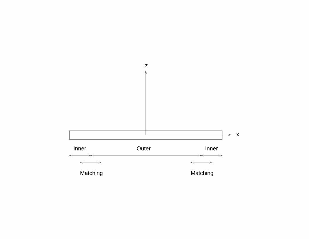
distribution in the strip. The geometry is illustrated in Fig. 1. The strip is in the x − y

plane, being infinite in the y-direction, and having a width 2a such that the strip occupies

4

the region −a < x < a. The applied field Ha(t) = Ha(t)z is normal to the strip and in the

z-direction. The vector potential A satisfies

−∇2A = 4πJ, (2.1)

in the transverse gauge in which ∇ ·A = 0. We will focus here on situations in which the

current density is invariant along the y-direction (along the length of the strip), so that

both J and A are along the y-direction. In the thin film approximation, the current density

Jy(x, z, t) is averaged over the thickness d of the film; the averaged current will be denoted

by j(x, t), so we have

Jy(x, z, t) = d j(x, t)δ(z)θ(a2 − x2). (2.2)

Eq. (2.1) is solved by introducing the Green’s function for the two dimensional Laplacian,

G(x− x′, z − z′):

Ay(x, z, t) = A0,y − 4π∫

G(x− x′, z − z′)Jy(x, z, t) dx′ dz′

= A0,y − 4πd∫ a

−aG(x− x′, z)j(x′, t) dx′. (2.3)

Differentiating both sides with respect to x, and using ∂A0,y/∂x = Ha(t), we obtain

Hz(x, z, t) =∂Ay(x, z, t)

∂x

= Ha(t)− 4πd∫ a

−a

∂G(x − x′, z)

∂xj(x′, t) dx′. (2.4)

Finally, if we specialize Eq. (2.4) to z = 0, and use ∂G(x − x′, 0)/∂x = 1/2π(x − x′), we

obtain for the magnetic field normal to the strip,

Hz(x, t) = Ha(t) + 2d(P )∫ a

−a

j(x′, t)

x′ − xdx′, (2.5)

where (P ) indicates a principle value integral.

To complete the description, we require a constitutive relation between the averaged

current and the fields. This paper will concentrate on the linear response of the current, so

that the general time-dependent response is

5

j(x, t) =∫ t

−∞σ(t− t′)Ey(x, t

′) dt′, (2.6)

with σ the conductivity. In most of this paper we shall be interested in the solution of the

initial value problem; i.e., the time evolution of the sheet current after an applied current

has been switched on. Then it is natural to Laplace transform the currents and the fields

with respect to time t:

j(x, s) =∫ ∞

0e−stj(x, t) dt, (2.7)

and so on. The inverse Laplace transform is

j(x, t) =1

2πi

∫ c+i∞

c−i∞estj(x, s) ds, (2.8)

with the integration contour chosen to pass to the right of any singularities. After Laplace

transforming, Eq. (2.10) becomes

j(x, s) = σ(s)Ey(x, s)

= −sσ(s)Ay(x, s), (2.9)

where Ey(x, t) = −∂Ay(x, t)/∂t and an integration by parts has been used to obtain the last

line. Now Laplace transform Eq. (2.5) with respect to time, and use Eq. (2.9) to eliminate

the fields in favor of the currents, to obtain the following equation of motion for the current:

− 4πλeff(s)d∂j(x, s)

∂x= Ha(s) + 2d (P )

∫ a

−a

j(x′, s)

x′ − xdx′, (2.10)

where λeff(s) is an effective screening length defined by

λeff(s) =1

4πdsσ(s). (2.11)

For a superconductor, σ(s) = 1/4πλ2s, with λ the London penetration depth, so that in this

case λeff = λ2/d. For an Ohmic conductor, λeff = 1/4πσ(0)ds = D/ds, with D the diffusion

constant for the magnetic flux. An Ohmic response would be realized in a normal metal or

in a type-II superconductor in the flux-flow regime. Eq. (2.10) is essentially identical to the

6

equations of motion derived by Larkin and Ovchinnikov [7], Eq. (33), and Brandt [1], Eq.

(3.6) the only difference being that Laplace rather than Fourier transforms are being used

here. This equation of motion can be conveniently expressed in dimensionless variables by

writing x′ = x/a, f(x′, s) = j(x, s)/(Ha(s)/2πd), and ǫ = 2λeff(s)/a:

− ǫf ′(x, s) = 1 +1

π(P )

∫ 1

−1

f(x′, s)

x′ − xdx′ (2.12)

(the s dependence of ǫ will be suppressed for notational simplicity; it will be reinstated later

when the transforms are inverted). The current density is the primary quantity of interest

in this paper. A related, and experimentally accessible, quantity is the magnetic moment

per unit length of the strip [1],

M(s) =∫ a

−ax j(x, s) dx

= −a2Ha

4dm(s) (2.13)

where m(s) is a dimensionless moment defined as

m(s) = −2h(s)

π

∫ 1

−1xf(x, s) dx, (2.14)

where h(s) is defined through Ha(s) = Hah(s).

There are no known analytical solutions of Eq. (2.12); its solution is the subject of the

remainder of this paper. However, for a typical sample ǫ ≪ 1, in which case the left hand

side of Eq. (2.12) constitutes a singular perturbation (the highest derivative is multiplied by

the small parameter), and we can bring to bear all of the techniques of asymptotic analysis

to solve this problem [4]. Before attempting this, we will first develop a perturbative analysis

which is valid for ǫ≫ 1, which is physically less interesting but mathematically simpler.

III. EXPANSION FOR LARGE ǫ

To study the behavior of Eq. (2.12) for large ǫ, it is useful to first rescale by introducing

a new function g(x, s) = ǫf(x, s). We then expand g(x, s) in powers of ǫ−1:

7

g(x, s) ∼ g0(x, s) + ǫ−1g1(x, s) + . . . . (3.1)

Substituting into Eq. (2.12) and matching terms of the same order, we have

g′0(x, s) = −1, (3.2)

g′1(x, s) = −1

π(P )

∫ 1

−1

g0(x′, s)

x′ − xdx′, (3.3)

and so on with the higher order terms. Assuming that there is no net current in the strip

(i.e., no applied current), then the current is odd in x, so that g(0) = 0, and we have

g0(x, s) = −x, (3.4)

g1(x, s) =1

π

[

x+1− x2

2ln(

1 + x

1− x

)

]

. (3.5)

The current increases linearly across the sample, except near the edges. Near the left edge

(x = −1), we have

g(x, s) ∼ 1− 1

πǫ[1 + (1 + x) ln(2/(1 + x))] . (3.6)

As we shall see below, a similar behavior near the edge will also emerge in the small-ǫ limit.

From the expansion for f(x, s) we can calculate the magnetic moment from Eq. (2.14):

m(s) = h(s)

[

4

3

1

πǫ(s)− 2

(πǫ(s))2+O(ǫ−3)

]

. (3.7)

For an Ohmic conductor, ǫ(s) = 2D/ads, so the magnetic moment vanishes linearly with

frequency at low frequency. This result is essentially equivalent to Eq. (5.6) of Ref. [1].

IV. ASYMPTOTIC ANALYSIS FOR SMALL ǫ

We now turn to the solution of Eq. (2.12) for small ǫ. An asymptotic solution can be

obtained using the method of matched asymptotic expansions. We break up the strip into

an “outer region,” which is the interior of the strip, and two “inner regions,” one near each

edge. This is illustrated schematically in Fig. 2. The solutions are then matched in common

overlap regions. A detailed discussion of the method can be found in Ref. [4].

8

A. Outer solution

The expansion in the outer region (away from the edges) is obtained by expanding f as

a series in ǫ:

f(x; ǫ) ∼ f0(x) + ǫf1(x) + . . . . (4.1)

Substituting this expansion into Eq. (2.12) and collecting terms of the same order, we find

for f0(x)

1

π(P )

∫ 1

−1

f0(x′)

x′ − xdx′ = −1. (4.2)

The solution of this singular integral equation which is odd is x can be found in Ref. [8]:

f0(x) = − x

(1 − x2)1/2, (4.3)

which coincides with the usual solution obtained from conformal mapping techniques. Near

the edges at x = ±1, f0 behaves as

f0 ∼ ∓ 1

[2(1∓ x)]1/2, (4.4)

so the current has a square root divergence at the edges. This is due to the fact that the

outer solution corresponds to complete screening of the applied field, which can only be

achieved by having an infinite current density at the edges. The outer solution therefore

breaks down at distances of order ǫ of the edges; the current at the edges is thus of order

ǫ−1/2. In order to remedy this problem, we proceed to the solution of the inner problem near

each of the edges.

B. Inner solution

We will first study the inner problem at the left edge, x = −1. The outer solution breaks

down at x+ 1 ∼ ǫ, suggesting that the appropriate variable in the inner region is

X = (x+ 1)/ǫ. (4.5)

9

Also, since f(−1) ∼ ǫ−1/2, we rescale f(x) in the inner region as

F (X) = ǫ1/2f(x), (4.6)

so that F (0) = O(1). In terms of these inner variables, Eq. (2.12) becomes

F ′ = −ǫ1/2 − 1

π(P )

∫ 2/ǫ

0

F (X ′)

X ′ −XdX ′. (4.7)

Next, expand F (X ; ǫ) in powers of ǫ1/2, as suggested by the rescaled form of the integro-

differential equation:

F (X ; ǫ) ∼ F0(X) + ǫ1/2F1(X) + . . . . (4.8)

The lowest order term satisfies

F ′0(X) = −1

π(P )

∫ 2/ǫ

0

F0(X′)

(X ′ −X)dX ′

= −1

π(P )

∫ ∞

0

F0(X′)

(X ′ −X)dX ′ +

1

π(P )

∫ ∞

2/ǫ

F0(X′)

(X ′ −X)dX ′. (4.9)

For small ǫ the second integral will be dominated by the large X behavior of F0(X); it will

be shown below that in order to match onto the outer solution this is necessarily of the form

F0(X) ∼ (2X)−1/2. Therefore, we see that the second integral is of order ǫ1/2, and can be

dropped at this order of the calculation. Our final integral equation for F0(X) is then

F ′0(X) = −1

π(P )

∫ ∞

0

F0(X′)

(X ′ −X)dX ′. (4.10)

The problem in the inner region consists of solving a homogeneous integro-differential equa-

tion on a semi-infinite interval. This is equivalent to finding the current distribution in a

semi-infinite strip in zero applied magnetic field.

Eq. (4.10) can be solved using the Wiener-Hopf method [8], as follows. The function

F0(X) → 0 as X → ∞, and F0(X) = 0 for X < 0; introduce a second unknown function

G(X) such that G(X) = 0 for X > 0 and G(X) → 0 as X → −∞. We then introduce the

complex Fourier transforms of F0(X) and G(X),

Φ+(k) =∫ ∞

0F0(X)eikXdX, (4.11)

10

G−(k) =∫ 0

−∞G(X)eikXdX, (4.12)

such that Φ+(k) is analytic for Im(k) > −β and G−(k) is analytic for Im(k) < α, for some

α > β. Then Fourier transforming Eq. (4.10), and integrating by parts, we obtain

G−(k)− F0(0)− ikΦ+(k) = isgn(k)Φ+(k). (4.13)

We see that as k → ∞,

Φ+(k) ∼ −F0(0)

ik+O(k−2). (4.14)

To take care of the ambiguities in defining sgn(k), replace it by k/(k2 + δ2)1/2, with the real

part > 0 for Re(k) > 0, and choose the branch cuts to run between (−i∞,−iδ) and (iδ, i∞).

We can then take δ → 0 at some later point in the calculation. Rearranging Eq. (4.13) a

bit, we have

ikK(k)Φ+(k) = G−(k)− F0(0), (4.15)

where

K(k) = 1 +1

(k2 + δ2)1/2. (4.16)

Now, if we can factor K(k) into the form K(k) = K+(k)/K−(k), with K+(k) analytic for

Im(k) > −δ and K−(k) analytic for Im(k) < δ, then we may rewrite Eq. (4.15) as

ikK+(k)Φ+(k) = K−(k) [G−(k)− F0(0)] . (4.17)

Both sides are now analytic in their respective regions of analyticity; we can then use analytic

continuation arguments to note that both sides must then equal an entire function E(k). By

examining the limiting behavior of the left hand side as k → ∞, we see that this function

must be chosen to be a constant C (any positive power of k would produce non-integrable

singularities in F0(X)), so that we finally have

Φ+(k) =C

ikK+(k). (4.18)

11

The function F0(X) is then obtained by inverting the Fourier transform,

F0(X) =1

2π

∫ ∞

−∞Φ+(k)e

−ikXdk, (4.19)

with the integration path indented so as to pass above any singularities on the real axis.

The only remaining task is the decomposition of K(k), which is carried out in Appendix

A. Using Eqs. (A4) and (A5), we have

F0(X) =C

2πi

∫ ∞

−∞

e−iϕ(k)

k(1 + 1/|k|)1/2 e−ikX dk

= −Cπ

∫ ∞

0

sin [kX + ϕ(k)]

(k2 + k)1/2dk, (4.20)

where the phase ϕ(k) is given by

ϕ(k) =π

4+

1

π

∫ k

0

ln u

1− u2du. (4.21)

The constant C is determined from the matching conditions, which are discussed below.

C. Asymptotic matching

The inner and outer solutions may now be matched together in a suitable overlap region.

This is done by expressing the outer solution f0(x) in terms of the inner variable X =

(x+ 1)/ǫ, and then taking X → 0 while holding ǫ fixed:

f0(X) = − ǫX − 1

[(2− ǫX)ǫX ]1/2

∼ 1

(2ǫX)1/2(X → 0). (4.22)

The inner solution F0(X) must match onto this outer solution as X → ∞, so the asymptotic

behavior of F0(X) must be

F0(X) ∼ 1

(2X)1/2(X → ∞). (4.23)

Now expand Eq. (4.20) for large-X ; the integral is dominated by the small-k behavior of the

integrand, and we find

12

F0(X) ∼ − C

(πX)1/2, (4.24)

so that we have

C = −(

π

2

)1/2

(4.25)

in order to match the inner and outer solutions. Therefore our final expression for the inner

solution is

F0(X) =1

(2π)1/2

∫ ∞

0

sin [kX + ϕ(k)]

(k2 + k)1/2dk. (4.26)

Comparing Eqs. (4.14) and (4.18), we see that F0(0) = −C = (π/2)1/2.

By rotating the integration contour, it is possible to show that for X < 0 the integral

vanishes (as it should), while for X > 0 the integral may be written as

F0(X) =1

(2π)1/2

∫ ∞

0

e−Xy−g(y)

y1/2(y2 + 1)3/4dy, (4.27)

with

g(y) =1

π

∫ y

0

ln u

1 + u2du. (4.28)

This function has the limiting behaviors

g(y) =

−y ln(e/y)/π +O(y3), y ≪ 1;

− ln(ey)/πy +O(y−3), y ≫ 1.(4.29)

The square-root singularity in the integrand at y = 0 can be removed by changing variables

to y = z2, so that

F0(X) =(

2

π

)1/2 ∫ ∞

0

e−Xz2−g(z2)

(z4 + 1)3/4dz, (4.30)

which is particularly convenient for numerical evaluation. As shown in Appendix B, for

small-X , F0(X) has the expansion

F0(X) =1

(2π)1/2

[

π − 1.4228X +X lnX +O(X2)]

(4.31)

13

(which disagrees with Eq. (37) of Larkin and Ovchinnikov, Ref. [7]; see the remarks in

Appendix B). Although the current is finite at X = 0, it has a slope which diverges as

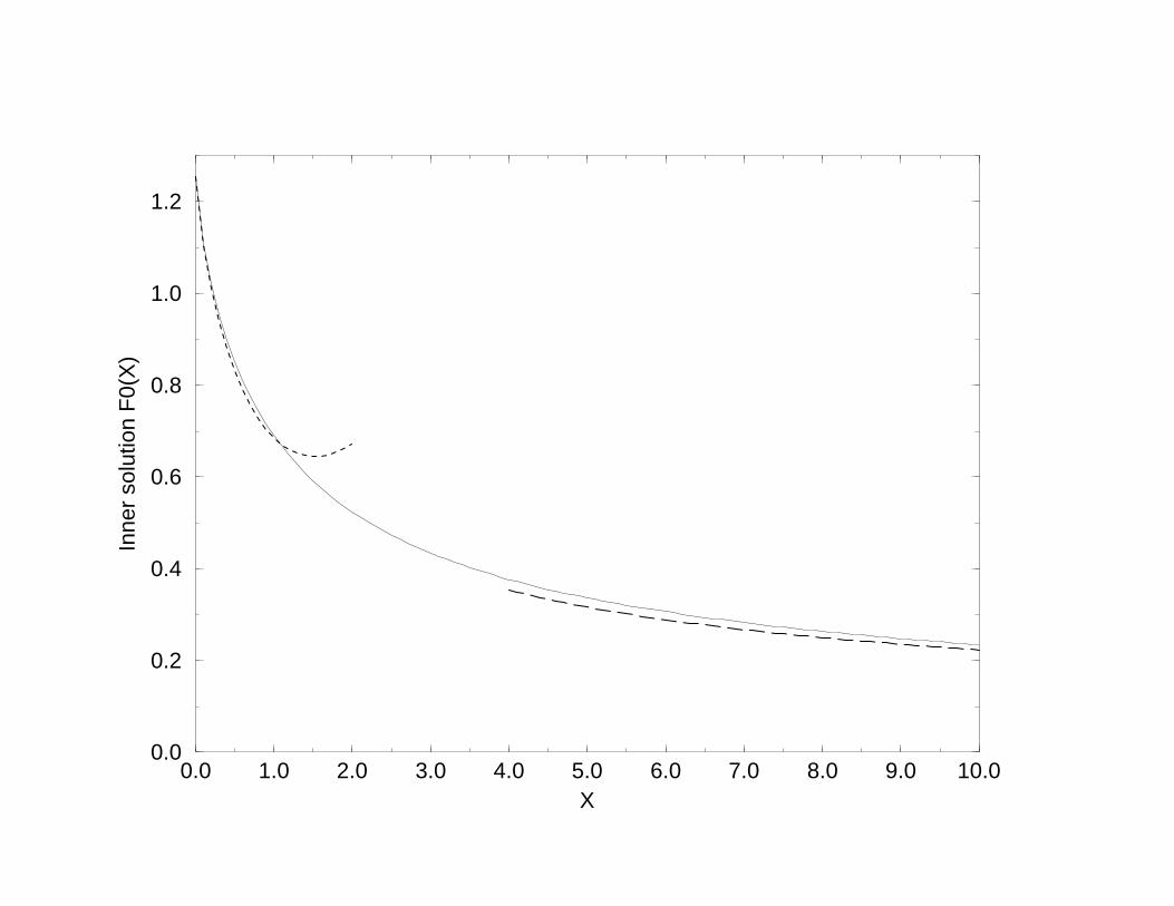
ln(X). The result of a numerical evaluation of the integral, along with a comparison of the

numerical results to the asymptotic expansions, is shown in Fig. 3.

So far we have only discussed the matching procedure at the left edge of the strip x = −1.

The same procedure can be carried out at the right edge, x = 1, as follows. At the right

edge, the inner variable will be X = (1 − x)/ǫ. As before, we will also rescale f(x) as

F (X) = ǫ1/2f(x). Substituting these expressions into Eq. (2.12), we obtain

F ′(X) = ǫ1/2 − 1

π(P )

∫ 2/ǫ

0

F (X ′)

X ′ − XdX ′, (4.32)

which is the same as Eq. (4.7) except for the minus sign in front of the ǫ1/2. Expanding

in powers of ǫ1/2, the O(1) term, F0(X), satisfies Eq. (2.12), and the method of solution is

identical. To match onto the outer solution, we write f0(x) in terms of X , and then take

X → 0 while holding ǫ fixed:

f0(X) = − 1− ǫX

[(2 − ǫX)ǫX ]1/2

∼ − 1

(2ǫX)1/2(X → 0). (4.33)

Therefore, the asymptotic behavior of F0(X) must be

F0(X) ∼ − 1

(2X)1/2(X → ∞). (4.34)

Therefore, F0(X) = −F0(X), which could have been surmised from the symmetry of the

problem.

D. Uniform solution

We are now in a position to construct an asymptotic solution which is uniformly valid

across the entire width of the strip; i.e., valid for all x as ǫ → 0. To do this we simply add

the inner and outer solutions; however, this would produce a result which was 2fmatch(x) in

14

the matching region, so we also need to subtract the fmatch(x) for each of the two matching

regions [4]. The result is

funif(x, s) = − x

(1− x2)1/2+

1

[2(1− x)]1/2− 1

[2(1 + x)]1/2

+ǫ(s)−1/2 {F0[(1 + x)/ǫ(s)]− F0[(1− x)/ǫ(s)]} . (4.35)

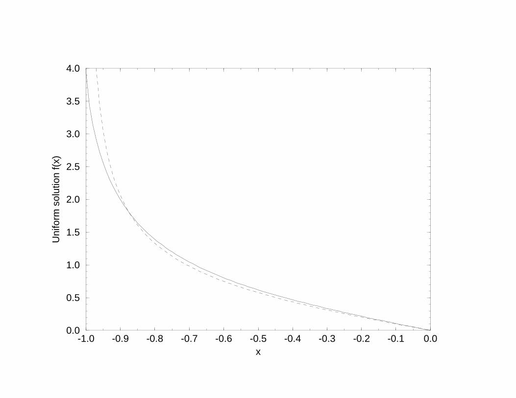
The uniform solution is plotted in Fig. 4 for ǫ = 0.1.

With the uniform solution we can calculate the magnetic moment, given in Eq. (2.14).

The result is

m(s) = h(s)

{

1− 8

3π+(

2

π

)3/2 ∫ ∞

0

e−g(ǫy)[(y + 1)e−2y + y − 1]

y5/2[1 + ǫ2y2]3/4dy

}

. (4.36)

For ǫ = 0, the integral is 8/3π, so that m(s) = h(s), which is the ideal screening limit.

Determining the leading ǫ behavior of the integral is rather subtle; the details are relegated

to Appendix C. The result is

m(s) = h(s)

[

1− 6

π2ln

(

8eγ−5/3

ǫ

)

ǫ

]

. (4.37)

This expression should give the correct high-frequency (s→ ∞) behavior of the magnetiza-

tion. Note that for s = 0 (ǫ → ∞), m(s) = 1 − 8/3π = 0.151; however, we know that the

correct limiting behavior is m(0) = 0 (see Sec. III). Therefore the uniform approximation

does not reproduce the correct low frequency behavior of the magnetization for an Ohmic

conductor.

V. MAGNETIC FIELD WITHIN THE STRIP

By using the constitutive relation, Eq. (2.9), it is also possible to calculate the magnetic

field perpendicular to the strip. Using Hz(x, s) = ∂Ay(x, s)/∂x, going to our dimensionless

variables, and using the uniform approximation from the section above, we have

Hz(x, s) = −Ha(s)ǫ(s)∂f(x, s)

∂x

= Ha(s)

{

ǫ(s)

[

1

(1− x2)3/2− 1

[2(1− x)]3/2− 1

[2(1 + x)]3/2

]

−ǫ(s)−1/2 {F ′0[(1 + x)/ǫ(s)] + F ′

0[(1− x)/ǫ(s)]}}

. (5.1)

15

The magnetic field is plotted in Fig. 5. From the results in Appendix B, close to the edges

(1± x = O(ǫ)) we have

F ′0(X) = − 1

(2π)1/2ln(1/X) + O(1), (5.2)

so that it would appear that the field diverges logarithmically at the edges, in agreement with

the numerical work in Ref. [1]. However, as we get even closer to the edge (1±x = O(ǫ3)), this

log divergence is swamped by a square-root divergence from the outer and overlap terms.

This latter behavior is most likely an artifact of the approximation, and would probably

disappear in a higher-order calculation.

VI. DYNAMICS OF THE CURRENT DENSITY AND MAGNETIZATION

Having obtained a uniformly asymptotic solution to the equation of motion for the av-

eraged current density, we can now examine its evolution in the time domain by inverting

the Laplace transform for j(x, s), Eq. (2.8). The details of the inversion process will depend

upon the time dependence of the applied field, and the model chosen for ǫ(s). Two different

models for ǫ(s) will be considered: (1) ǫ(s) = 2λ2/ad a constant, corresponding to a super-

conductor; (2) ǫ(s) = (2D/ad)(1/s), with D = 1/4πσ(0) the diffusion constant for flux in

the normal phase, corresponding to an Ohmic conductor (a type-II superconductor in the

flux-flow regime, for instance [1]).

A. Superconductor

For a superconductor the inversion of the Laplace transform is particularly simple. In

conventional units we have (recall that λeff = λ2/d)

junif(x, t) =Ha(t)

2πd

− x

(1− x2)1/2+

[

1

2(1− x)

]1/2

−[

1

2(1 + x)

]1/2

ǫ−1/2[

F0

(

1 + x

ǫ

)

− F0

(

1− x

ǫ

)]}

. (6.1)

In this case the induced current is in phase with the applied field.

16

B. Ohmic conductor: penetration of a jump in the applied field

We will first treat the case in which the field is suddenly switched on, so that Ha(t) =

Haθ(t), and thus Ha(s) = Ha/s. Inverting the Laplace transform, we have

junif(x, t) =Ha(t)

2πd

− x

(1− x2)1/2+

[

1

2(1− x)

]1/2

−[

1

2(1 + x)

]1/2

+jedge(1 + x, t)− jedge(1− x, t), (6.2)

where the edge current jedge(x, t) is given by

jedge(x, t) =Ha

2πd

(

ad

4D

)1/2∫ ∞

0

e−g(y)

y1/2(y2 + 1)3/4dy

× 1

2πi

∫ c+i∞

c−i∞

exp[st− (adx/2D)ys]

(πs)1/2ds. (6.3)

The Laplace transform can be calculated by closing the contour in the left half plane (for

t > dx/2D), wrapping the contour around the branch cut along the negative s axis, with

the result

jedge(x, t) =Ha

2πd

(

ad

4Dt

)1/2

F1

(

ad

2D

x

t

)

, (6.4)

where F1(u) is a scaling function given by

F1(u) =1

π

∫ 1/u

0

e−g(y)

(1− uy)1/2y1/2(y2 + 1)3/4dy. (6.5)

The scaling function has been normalized so that F1(0) = 1; for large-u, F1(u) ∼ u−1/2.

For numerical purposes, it is useful to transform the integral by making the substitution

1− uy = sin2 θ, so that

F1(u) =2u

π

∫ π/2

0

exp[−g(cos2 θ/u)](cos4 θ + u2)3/4

dθ, (6.6)

which removes the square-root singularities from the integrand at the endpoints of integra-

tion.

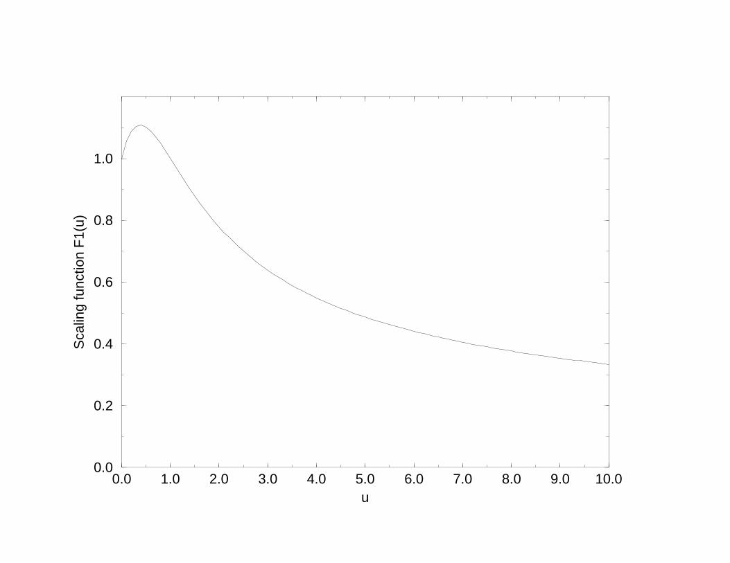
The scaling function F1(u) is plotted in Fig. 6. There is a maximum at u = 0.386,

with F1,max = 1.1078. From the position of this peak we can define a velocity v of flux

penetration:

17

v =(

x

t

)

max= 0.772

D

d. (6.7)

These results agree exactly with the numerical work of Brandt [1,2]. As noted by Brandt,

in the thin film geometry the flux entry is ballistic rather than diffusive, as it would be in a

bulk sample with no demagnetizing fields.

We can also calculate the time dependent magnetization after a jump in the field. By

using the small-ǫ expansion in Eq. (4.37), and inverting the Laplace transform by wrapping

the integration contour around the branch cut along the negative-s axis, we find at short

times

m(t) = 1− 6

π3(t/τ) ln(8πe−2/3t/τ) +O(t2), (6.8)

where τ = ad/2πD is a characteristic relaxation time. Similar behavior was found by Brandt

[1] in his numerical studies of the magnetization; for the prefactor of the log he obtained

0.205, compared to the present value of 6/π3 = 0.194; for the constant inside the log, he

obtained 25, compared to our value of 8πe−2/3 = 12.9. It is not clear whether these small

discrepancies are the result of the approximations in this paper or uncertainties in Brandt’s

numerical work.

C. Ohmic conductor: ac response

Next, we consider the response of the strip to an ac magnetic field, Ha(t) = Ha exp(iωt),

so that Ha(s) = Ha/(s− iω). When inverting the Laplace transform, there will be contri-

butions both from the pole at iω and from the square-root branch cut along the negative-s

axis. The branch cut contribution decays as t−1/2; since we are concerned here with the

steady-state behavior, we will neglect this term, keeping only the pole contribution. Writing

jedge(x, t) = jedge(x, ω) exp(iωt), we have for the current near the edge

jedge(x, ω) =Ha

2πd

(

ωπad

8D

)1/2

F2

(

dωx

2D

)

, (6.9)

where the ac scaling function F2(u) is given by

18

F2(u) =

√2

π

∫ ∞

0

e−g(y)−iuy+iπ/4

y1/2(y2 + 1)3/4dy. (6.10)

The scaling function is defined so that ReF2(0) = ImF2(0) = 1. The real and imaginary

parts of the ac scaling function are plotted in Fig. 7. The real part of the scaling function

has a maximum at u = 0.232 (xω = 0.0738 a/τ in conventional units), with ReF2,max =

1.0787; the imaginary part changes sign at u = 2.43 (xω = 0.773 a/τ in conventional units).

These results are once again very close to Brandt’s numerical results [1,2]. The uniform

approximation to the current density is

junif(x, ω) =Ha

2πd

− x

(1− x2)1/2+

[

1

2(1− x)

]1/2

−[

1

2(1 + x)

]1/2

+jedge(1 + x, ω)− jedge(1− x, ω). (6.11)

Using the small-ǫ expansion of the magnetization, Eq. (4.37), we can also calculate the

high frequency magnetization; the result is

m(ω) = 1− 6

π3

ln(8πeγ−5/3iωτ)

iωτ+O(ω−2), (6.12)

which is quite similar to the numerical result obtained by Brandt [1]. The constants differ

slightly; here the prefactor is 0.194, while Brandt obtained 2/π2 = 0.203; for the constant

inside the log, Brandt obtained 16.2, compared to the present value of 8πeγ−5/3 = 8.45.

VII. EXTENSIONS OF THE METHOD

With minor modifications it is also possible to treat two related problems, the current

distribution in a thin superconducting disk in a perpendicular field, and the current distri-

bution in a thin strip in the presence of an applied current. Rather than discussing these

cases in detail, only a brief sketch of the results will be provided.

A. Disk geometry

Rather than a strip we now have a superconducting disk centered at the origin of the

x − y plane, of radius a. The current density and the vector potential are both in the φ

19

direction. Using a Green’s function method similar to that in Sec. II, the z-component of

the magnetic field inside the disk satisfies

Hz(r, z = 0, t) = Ha(t) + 2d(P )∫ a

0P (r, r′)j(r′, t) dr′, (7.1)

where the kernel P (r, r′) is given by [2]

P (r, r′) =K(k)

r + r′+E(k)

r′ − r, k2 =

4rr′

(r + r′)2, (7.2)

where K(k) and E(k) are complete elliptic integrals of the first and second kind. We

again Laplace transform, use the constitutive relation between j and A, and go to the

dimensionless variables r′ = r/a, f(r, s) = j(r, s)/(Ha(s)/π2d), and ǫ(s) = 2λeff/a, to arrive

at the following integro-differential equation:

− ǫ1

r

∂

∂r[rf(r, s)] =

π

2+

1

π(P )

∫ 1

0P (r, r′)f(r′, s)dr′. (7.3)

The outer solution is [8,2]

f0(r) =r

(1− r2)1/2, (7.4)

which has a square root singularity at the edge. Near the edge we construct the inner

solution by defining the inner variables R = (1 − r)/ǫ, F (R) = ǫ1/2f(r); for small ǫ the

kernel behaves as

P (1− ǫR, 1− ǫR′) =1

ǫ

1

R−R′+O(ln ǫ). (7.5)

After expanding F (R; ǫ) in ǫ, we find that the lowest order term satisfies Eq. (4.10), so that

the inner solution is the same as before. Finally, the inner and outer solutions are matched

as before; the uniform solution is then

funif(r, s) =r

(1− r2)1/2− 1

[2(1− r)]1/2+ ǫ(s)−1/2F0[(1− r)/ǫ(s)]. (7.6)

The magnetic moment of the disk is

M(s) = π∫ a

0r2j(r, s) dr

=2a3Ha

3πdm(s), (7.7)

20

where the dimensionless moment in the disk geometry is

m(s) =3h(s)

2

∫ 1

0r2f(r, s) dr. (7.8)

Using the uniform approximation, this becomes

m(s) = h(s)

{

1− 4√2

5+

3

2√2π

∫ ∞

0

e−g(ǫy) [y2 − 2y + 2− 2e−y]

y7/2(1 + ǫ2y2)3/4

}

. (7.9)

For small ǫ the integral can be expanded using the same method as for the strip (see Ap-

pendix C), with the result

m(s) = h(s)

[

1− 2√2

πln

(

4eγ−5/3

ǫ

)

ǫ+O(ǫ2)

]

. (7.10)

For an Ohmic conductor ǫ(s) = 2D/ads = 1/πτs, with τ = ad/2πD. After inverting the

Laplace transform, we find that after a jump in the magnetic field, the magnetization for

small t is

m(t) = 1− 2√2

π2(t/τ) ln

(

4πe−2/3t/τ)

, (7.11)

while the ac magnetization at high frequencies is

m(ω) = 1− 2√2

π2

ln(4πeγ−5/3iωτ)

iωτ. (7.12)

The behavior is essentially the same as for the strip, with slightly different constants. Similar

behavior has been found by Brandt [2] in his numerical studies. He finds a prefactor of

3/π2 = 0.304, compared to the present value of 0.286; for the constant inside the log, he

obtains 11.3, compared to our 4.23. As in the strip geometry, the source of the discrepancy

is unclear.

B. Current distribution in the presence of an applied current

The effect of an applied transport current is to modify the O(1) outer solution, which

now becomes

21

f0(x) = − x− fa(1− x2)1/2

, (7.13)

where fa = I(s)/(Ha(s)a/2), with I(s) the total current (not the current density) in the

strip. Writing the outer solution in terms of the inner variable X , we see that the matching

conditions are

f0(X) = ±(1± fa)1

(2ǫX)1/2, (7.14)

with the + corresponding to the left edge and the − to the right edge. The solution to the

inner problem is the same as before. After matching the inner and outer solutions, we have

for the uniform solution

funif(x, s) = − x− fa(1 − x2)1/2

+1− fa

[2(1− x)]1/2− 1 + fa

[2(1 + x)]1/2

+ǫ(s)−1/2 {(1 + fa)F0[(x+ 1)/ǫ(s)]− (1− fa)F0[(1− x)/ǫ(s)]} . (7.15)

With this expansion it is possible to study the time-dependent response, just as in the zero

current case.

VIII. LONG TIME BEHAVIOR AFTER A JUMP IN THE APPLIED FIELD

All of the previous sections have been concerned with the short-time or high frequency

response of a strip to an applied field. In this section we will treat the long-time relaxation

of the current density in an Ohmic strip after a jump in the perpendicular field. We will

again use the method of matched asymptotic expansions, but in a slightly different form.

We start with the equation of motion for the magnetic field, Eq. (2.5), and differentiate

with respect to time t. The time derivative of the magnetic field can be related to the

current density for an Ohmic conductor with conductivity σ through ∂Hz/∂t = −∂Ey/∂x =

−σ−1∂j/∂x. Since the applied field is a step function, ∂Ha(t)/∂t = Haδ(t). Therefore, for

t > 0 the current density satisfies (using a as the unit of length)

− 1

aσ

∂j(x, t)

∂x= 2d(P )

∫ 1

−1

1

x′ − x

∂j(x′, t)

∂tdx′. (8.1)

22

Following Brandt [1,2], write the current density as an eigenfunction expansion:

j(x, t) =Ha

2πd

∑

n

cnψn(x)e−t/τn , (8.2)

where the the relaxation times τn = ad/2Dλn are related to the eigenvalues λn, which follow

from the solution of

dψn(x)

dx=λnπ(P )

∫ 1

−1

ψn(x′)

x′ − xdx′. (8.3)

This equation is similar to the homogeneous version of the integral equation for the current

density, Eq. (2.12), but with an important sign difference on the left hand side. As a result,

we can expect the eigenfunctions to be oscillatory, rather than decaying, in the middle of

the strip. The long time behavior of the current density will be controlled by the smallest

eigenvalue λ0, which produces the longest relaxation time τ0.

We can develop an asymptotic analysis of the eigenvalue spectrum by first assuming that

λn ≫ 1, so that 1/λn serves as our small parameter. The consistency of this assumption

should be checked at the end of the calculation. As before, we break the problem up into an

outer problem in the middle of the strip, and two inner problems near each of the two edges.

First we treat the outer problem. Define the outer variables Xo = λnx, Ψ(o)n (Xo) = ψn(x).

Then the integral equation for the outer function is

dΨ(o)n (Xo)

dXo=

1

π(P )

∫ λn

−λn

Ψ(o)n (X ′

o)

X ′o −Xo

dX ′o. (8.4)

Taking λn → ∞, we then have an integro-differential equation which relates the derivative

of a function to its Hilbert transform. The solutions are cos(Xo) and sin(Xo); however, in

the absence of an applied current the current density must be odd in x, so the physically

acceptable solution is

Ψ(o)n (Xo) = An sin(Xo), (8.5)

with An a constant which can in principle depend upon n. This outer solution must be

matched onto the inner solution, which we turn to next.

23

Let’s first consider the inner problem at the left edge. Define the inner variables Xi =

λn(1+x) and Ψ(i)n (Xi) = ψn(x). Writing Eq. (8.3) in terms of the inner variables, and taking

λn → ∞, we have

dΨ(i)n (Xi)

dXi

=1

π(P )

∫ ∞

0

Ψ(i)n (X ′

i)

X ′i −Xi

dX ′i. (8.6)

which is once again an integral equation of the Wiener-Hopf type. To solve, introduce an

unknown function G(Xi) such that G(Xi) = 0 forXi > 0, and introduce the complex Fourier

transforms

Φ+(k) =∫ ∞

0Ψ(i)

n (Xi)eikXidXi, (8.7)

G+(k) =∫ ∞

0G(Xi)e

ikXidXi, (8.8)

such that Φ+(k) is analytic for Im(k) > −β and G+(k) is analytic for Re(k) < α, for some

α > β. Fourier transforming Eq. (8.6), we then obtain

G+(k)−Ψ(i)n (0) = ikK(k)

(

k2 − k20k2 + δ2

)

Φ+(k), (8.9)

where

K(k) =k2 + δ2

k2 − k20

[

1− 1

(k2 + δ2)1/2

]

, (8.10)

with δ a small parameter which is taken to zero at some convenient point of the calculation,

and k0 = (1 − δ2)1/2. The kernel K has been constructed so that it is free of zeros in the

strip −δ < Im(k) < δ, and K(k) → 1 as |k| → ∞. The kernel can be factored into the

quotient form K = K+/K− using the general factorization procedure (see Appendix A),

with the result that

K+(k) = [K(k)]1/2eiϕ(k), (8.11)

ϕ(k) = −kπ

∫ ∞

0

ln[K(x)/K(k)]

x2 − k2dk. (8.12)

24

With the factorization, Eq. (8.9) can be written as

(k − iδ)K−(k)[G+(k)−Ψ(i)n (0)] = ik

(

k2 − k20k + iδ

)

K+(k)Φ+(k). (8.13)

Both sides are analytic in their respective regions of analyticity; analytic continuation allows

us to set both sides equal to an entire function E(k). To choose E(k), we require that

Ψ(i)n (0) be finite, so that Φ+(k) ∼ 1/k for large k. This can only be achieved by taking

E(k) = Bnk/21/2, with Bn a constant (the 21/2 has been added to simplify some of the

resulting expressions). Therefore,

Φ+(k) =Bn

21/2k + iδ

i(k2 − k20)K+(k). (8.14)

Now we invert the Fourier transform, with the integration path passing above the poles on

the real axis. Closing the contour in the lower half plane, we pick up contributions from the

poles and from a branch cut which runs along the Im(k) < 0 axis, with the final result

Ψ(i)n (Xi) = −Bn cos(Xi − π/8) +Bnψcut(Xi), (8.15)

where ψcut(Xi) is the contribution from the branch cut, which is O(X−3/2i ) for large Xi.

We must now match together our outer solution, Eq. (8.5), and our inner solution, Eq.

(8.15). Taking the outer limit of the inner solution, and rewriting Xo and Xi in terms of x,

we find that

− Bn cos[λn(1 + x)− π/8] = An sin(λnx). (8.16)

This is only satisfied if λn−π/8 = (n+1/2)π and An = (−1)nBn. Therefore, the eigenvalue

spectrum is

λn =5π

8+ nπ, n = 0, 1, 2, . . . . (8.17)

The same matching procedure must also be carried out at the right edge, and the analysis

is identical. From the inner and outer solutions we can construct a uniform solution, which

is

25

ψn,unif(x) = sin [(n+ 5/8)πx] + (−1)n {ψcut[λn(1 + x)]− ψcut[λn(1− x)]} , (8.18)

where an overall constant has been dropped.

This asymptotic expansion should be accurate for large n. To compare these results

to Brandt’s numerical work [1,2], first note that Brandt calculates Λn = λn/π, so we find

Λ0 = 5/8 = 0.625. Brandt obtains the numerical value of Λ0 = 0.638, which is within 2% of

the result of our asymptotic analysis. The approximation only improves for large n, so our

result appears to be quite accurate for all n. This due in part to the fact that λ0 = 5π/8 is

large enough for the asymptotic analysis to be effective. With regard to the eigenfunctions,

for large n the cut contributions become less significant (their contribution is localized near

the edges), and so ψn(x) = sin [(n+ 5/8)πx] becomes an accurate approximation to the

eigenfunctions. Based on his numerical results, Brandt quotes a similar result, but with

5/8 replaced by 1/2; our result should provide a better approximation, and even appears

to resemble the numerical result for n = 0. The cut contributions have derivatives which

diverge logarithmically at the edges, similar to the numerical solutions.

IX. DISCUSSION AND SUMMARY

By applying the method of matched asymptotic expansions to the integro-differential

equation for the current density in the strip, Eq. (2.12), we have been able to derive a uniform

approximation for the current density, which has been used to study the nonequilibrium

response of the current in the strip, as well as the ac current density and the magnetization.

Most of the effort has gone into understanding the response of an Ohmic strip. However,

the method is easily generalized to more complicated dispersive conductivities σ(s); the only

difficulties arise in inverting the Laplace transform to obtain the temporal response. For the

purely Ohmic response, we found that after a jump in the perpendicular magnetic field the

current propagates in from the edges at a constant velocity, in contrast to the longitudinal

case, where the current propagates diffusively [1]. The difference is due to the demagnetizing

effects in the perpendicular geometry; initially the field lines must bend around the edges

26

of the sample, resulting in a large magnetic “pressure” which drives the current into the

sample.

A number of simplifying assumptions were made in order to make this problem analyti-

cally tractable. The most important is the assumption of linear response. For many type-II

superconductors, however, the current-voltage characteristics are highly nonlinear due to the

collective pinning of the flux lines. In the perpendicular geometry there has recently been

some progress in incorporating pinning (nonlinear response) into calculations of the current

and field patterns for thin superconducting strips [9,10]. It is possible that the asymptotic

methods used in this paper would be useful for studying the nonequilibrium, nonlinear re-

sponse in the perpendicular geometry. A second assumption is that the current in the strip

does not vary in the y-direction, so that we have an essentially one-dimensional problem. It

would be interesting to include small variations of the current along the y-direction in order

to determine the stability of the current fronts which enter after a jump in the perpendicular

field; this problem might also be amenable to the type of analysis discussed in this paper.

ACKNOWLEDGMENTS

I would like to thank Dr. Chung-Yu Mou for helpful discussions and for his assistance

in preparing several of the figures. This work was supported by NSF Grant DMR 92-23586,

as well as by an Alfred P. Sloan Foundation Fellowship.

APPENDIX A: DECOMPOSITION OF THE KERNEL K

We want to decompose the kernel K(k) given in Eq. (4.16) into K+(k)/K−(k), with K+

analytic in the upper half plane and K− analytic in the lower half plane. Since K(k) is free of

zeros in the strip −δ < Im(k) < δ and approaches 1 as k → ±∞, lnK(k) is analytic in this

strip and approaches 0 as k → ±∞. We can therefore perform an additive decomposition of

lnK(k) = lnK+(k)− lnK−(k) (A1)

27

by writing [8]

lnK+(k) =1

2πi

∫ ∞−iα

−∞−iα

lnK(z)

z − kdz, (A2)

with α > δ; there is an analogous expression for K−(k). This integral will be analytic for

Im(k) > −δ. Now if k can be taken to be real, and the integration path coincides with the

real axis (indented to pass under the pole at k), then

lnK+(k) =1

2lnK(k) +

k

πi

∫ ∞

0

ln[K(x)/K(k)]

x2 − k2dx, (A3)

where K(−x) = K(x) has been used to simplify the integral. Therefore, our decomposition

of K = K+/K− is (letting δ → 0)

K±(k) =

[

1 +1

|k|

]±1/2

eiϕ(k), (A4)

with

ϕ(k) =sgn(k)

π

∫ ∞

0ln

[

u(|k|+ 1)

|k|u+ 1

]

du

u2 − 1. (A5)

The last integral may be rewritten in a more convenient form by first differentiating with

respect to k, integrating with respect to u, and finally integrating with respect to k:

ϕ(k) =sgn(k)

π

∫ |k|

0

ln u

1− u2du+

π

4sgn(k). (A6)

This integral can be expressed in terms of dilogarithm functions, but this is not particularly

useful for our purposes.

For large |k|, ϕ(k) has the asymptotic expansion

ϕ(k) ∼ +1

π

ln(e|k|)k

+O(k−3), (A7)

while for small k, ϕ(k) has the series expansion

ϕ(k) =π

4sgn(k)− 1

πln(e/|k|)k +O(k3). (A8)

28

APPENDIX B: SMALL X BEHAVIOR OF F0(X)

In this Appendix the behavior of F0(X) for small X will be derived by using the method

of matched asymptotic expansions to derive a uniformly valid expansion for the integrand

of F0(X). Call the integrand in Eq. (4.27) I(y,X):

I(y,X) =e−Xy−g(y)

y1/2(y2 + 1)3/4. (B1)

Expanding for small X ,

Ii(y,X) =e−g(y)

y1/2(y2 + 1)3/4− y1/2e−g(y)

(y2 + 1)3/4X +O(X2). (B2)

This constitutes our inner expansion, which breaks down when Xy = O(1). To derive the

outer expansion, define an outer variable Y = Xy, rewrite I(y,X) in terms of Y , and expand

to lowest order in X :

Io(Y,X) =e−Y−g(Y/X)

Y 1/2(Y 2 +X2)3/4X2

=e−Y

Y 2X2 +O(X3). (B3)

In order to match the two expansions, express the inner expansion Ii(y,X) in terms of the

outer variable Y , and expand for small X :

Ii(Y/X,X) =e−g(Y/X)

Y 1/2(Y 2 +X2)3/4X2 − Y 1/2e−g(Y/X)

(Y 2 +X2)3/4X2

=[

1

Y 2− 1

Y

]

X2. (B4)

On the other hand, if we express the outer expansion Io(Y,X) in terms of the inner variable

y, we have

Io(Xy,X) =e−Xy

y2

=1

y2− X

y. (B5)

We see that the 1 term outer expansion of the 2 term inner expansion is equal to the 2 term

inner expansion of the 1 term outer expansion, in agreement with the van Dyke matching

29

principle [3]. To obtain the uniform expansion, add the inner and outer expansions, and

subtract the overlap:

Iunif(y,X) =e−g(y)

y1/2(y2 + 1)3/4− y1/2e−g(y)

(y2 + 1)3/4X +

e−Xy

y2− 1

y2+X

y+O(X2)

=e−g(y)

y1/2(y2 + 1)3/4− y1/2[e−g(y) − 1]

(y2 + 1)3/4X

+e−Xy − 1

y2+X

y− Xy1/2

(y2 + 1)3/4+O(X2). (B6)

To obtain the small X behavior of F0(X), we can integrate Iunif(y,X) on y. From the

arguments given in Sec. IV.C, we know that F0(0) = (π/2)1/2, so the first integral is

∫ ∞

0

e−g(y)

y1/2(y2 + 1)3/4dy = π. (B7)

The second integral must be evaluated numerically, with the result

−X∫ ∞

0

y1/2[e−g(y) − 1]

(y2 + 1)3/4dy = −0.7457X. (B8)

The last three integrals require some care. The third integral is logarithmically divergent

for small y, so integrate down to a cutoff a, and take a→ 0 at a later point:

∫ ∞

a

e−Xy − 1

y2dy = −(1− γ)X +X ln(a) +X ln(X) +O(a), (B9)

with γ = 0.5772 . . .. The last two integrals are logarithmically divergent for large y (the two

logs will cancel), so integrate up to A and then take A → ∞. For the fourth integral we

then have

X∫ A

a

dy

y= X [ln(A)− ln(a)]. (B10)

The fifth integral converges for small y, so we can extend the lower limit of integration to 0.

By integrating by parts, we can extract the leading ln(A) behavior; there is one remaining

integral which must be calculated numerically, with the result

−X∫ A

0

y1/2

(y2 + 1)3/4dy = −X [ln(A) + ln(2)− 0.4388]. (B11)

30

Adding Eqs. (B7)–(B11) together, we see that the dependence upon a and A drops out, as

it should, and we finally obtain

F0(X) =1

(2π)1/2

∫ ∞

0

e−Xy−g(y)

y1/2(y2 + 1)3/4dy

=1

(2π)1/2

[

π − 1.4228X +X lnX +O(X2)]

. (B12)

This is slightly different from Eq. (37) of Larkin and Ovchinnikov [7], which in our notation

is

F Larkin0 (X) =

1

(2π)1/2

[

π − ln(4e−γ)X +X lnX +O(X2)]

=1

(2π)1/2

[

π − 0.8091X +X lnX +O(X2)]

. (B13)

The difference between these two expressions becomes significant for values of X near 1.

For instance, numerically we find F0(1) = 1.732, while Eq. (B12) gives 1.718, a difference of

only 0.8%; the Larkin and Ovchinnikov expression gives 2.332, an error of 35%. The reason

for the discrepancy is not clear, since the derivation of their result appears not to have been

published.

APPENDIX C: SMALL ǫ BEHAVIOR OF THE MAGNETIZATION

In this Appendix we will determine the small-ǫ behavior of the dimensionless magne-

tization, m(s), given by Eq. (4.36), using the method of matched asymptotic expansions.

The derivation is quite analogous to derivation of the small X behavior of F0(X) which was

discussed in Appendix B. Call the integrand in Eq. (4.36) J(y, ǫ):

J(y, ǫ) =e−g(ǫy)[(y + 1)e−2y + y − 1]

y5/2[1 + ǫ2y2]3/4. (C1)

Expand for small-ǫ, using the small-x behavior of g(x) given in Eq. (g(y)), to obtain the

inner expansion:

Ji(y, ǫ) =(y + 1)e−2y + y − 1

y5/2

[

1 + (y/π) ln(e/ǫy)ǫ+O(ǫ2)]

. (C2)

31

This expansion breaks down when ǫy = O(1). To derive the outer expansion, define an outer

variable Y = ǫy, rewrite J(y, ǫ) in terms of Y , and expand to lowest order in ǫ:

Jo(Y, ǫ) =e−g(Y )

Y 3/2(1 + Y 2)3/4ǫ3/2 +O(ǫ5/2). (C3)

To match the two expressions, write the inner expansion Ji(y, ǫ) in terms of the outer variable

Y and expand for small ǫ:

Ji(Y/ǫ, ǫ) = Y −3/2 [1 + (Y/π) ln(e/Y )] ǫ3/2. (C4)

Next, take the outer expansion Jo(Y, ǫ) and write it in terms of the inner variable y and

expand for small ǫ:

Jo(ǫy, ǫ) = y−3/2 [1 + (y/π) ln(e/ǫy)ǫ] . (C5)

Again, we see that the 2 term inner expansion of the 1 term outer expansion is equal to the

1 term outer expansion of the 2 term inner expansion [3]. To obtain the uniform expansion

(i.e., an expansion valid for arbitrary y and small-ǫ), add the inner and outer expansions,

and subtract the overlap:

Junif(y, ǫ) =(y + 1)e−2y + y − 1

y5/2+ (1/π) ln(e/ǫy)

(y + 1)e−2y − 1

y3/2ǫ

+e−g(ǫy) − 1

y3/2(1 + ǫ2y2)3/4+ y−3/2

[

1

(1 + ǫ2y2)3/4− 1

]

. (C6)

We must now integrate Junif(y, ǫ) over y. For the first term we have

∫ ∞

0

(y + 1)e−2y + y − 1

y5/2dy =

2(2π)1/2

3. (C7)

For the second term we have two integrals:

ln(e/ǫ)

π

∫ ∞

0

(y + 1)e−2y − 1

y3/2dy = − 3

(2π)1/2ǫ ln(e/ǫ), (C8)

− ǫ

π

∫ ∞

0ln y

(y + 1)e−2y − 1

y3/2dy = −

(

2

π

)1/2 [

−4 +9

2ln 2 +

3

2γ]

ǫ. (C9)

32

The fourth and fifth integrals are both O(ǫ1/2), as can be seen by rescaling the integration

variable. The fourth integral was performed numerically, with the result

ǫ1/2∫ ∞

0

e−g(x) − 1

x3/2(1 + x2)3/4dx = 2ǫ1/2, (C10)

where the factor of 2 was determined to an accuracy of 1 part in 108. The last integral is

ǫ1/2∫ ∞

0x−3/2

[

1

(1 + x2)3/4− 1

]

dx = −2ǫ1/2. (C11)

We see that for all purposes the last two integrals sum to zero, although this has not been

proven analytically. Collecting together the other terms, we finally have

∫ ∞

0

e−g(ǫy)[(y + 1)e−2y + y − 1]

y5/2[1 + ǫ2y2]3/4=

2(2π)1/2

3

[

1− 9

4πln

(

8eγ−5/3

ǫ

)

ǫ+O(ǫ2)

]

. (C12)

A numerical evaluation of the integral for ǫ = 1 gives 0.49577; the expansion at ǫ = 1 gives

0.48624, an error of about 2%. We see that the expansion is quite accurate even for relatively

large values of ǫ.

33

REFERENCES

∗ Electronic address: atd2h@virginia.edu

[1] E. H. Brandt, Phys. Rev. B 49, 9024 (1994).

[2] E. H. Brandt, Phys. Rev. B 50, 4034 (1994).

[3] M. van Dyke, Perturbation Methods in Fluid Mechanics (Parabolic Press, Stanford CA,

1975).

[4] C. M. Bender and S. A. Orszag, Advanced Mathematical Methods for Scientists and

Engineers (McGraw-Hill, New York, 1978).

[5] A. T. Dorsey, Ann. Phys. 233, 248 (1994); J. C. Osborn and A. T. Dorsey, Phys. Rev.

B 50, 15 961 (1994).

[6] S. J. Chapman, Quart. Appl. Math. (to be published).

[7] A. I. Larkin and Yu. N. Ovchinnikov, Sov. Phys. JETP 34, 651 (1972).

[8] G. F. Carrier, M. Krook, and C. E. Pearson, Functions of a Complex Variable (Hod

Books, Ithaca, New York, 1983), pp. 376–432.

[9] E. Zeldov, J. R. Clem, M. McElfresh, and M. Darwin, Phys. Rev. B 49, 9802 (1994).

[10] T. Schuster, H. Kuhn, E. H. Brandt, M. Indenbom, M. R. Koblischka, and M. Kon-

czykowski, Phys. Rev. B 50, 16 684 (1994).

34

FIGURES

FIG. 1. Illustration of the film geometry considered in this paper. The film has a width 2a in

the x-direction, and a thickness d. The applied field Ha is in the z-direction.

FIG. 2. Schematic diagram of the outer, inner, and matching regions used in the small-ǫ asymp-

totic analysis.

FIG. 3. The inner solution F0(X, s), calculated from Eq. (4.30) (solid line). Also shown are the

asymptotic expansions for small X (dotted line) and large X (dashed line).

FIG. 4. Uniform approximation funif(x, s) to the current density for ǫ = 0.1, from Eq. (4.35)

(solid line). Since the current density is odd in x only the current density over half the strip is

shown. For comparison the ideal screening case (the outer solution f0(x) = −x/(1−x2)1/2 ) is also

shown (dashed line). At the left edge we have funif(x = −1) = 3.948.

FIG. 5. Perpendicular component of the magnetic field Hz(x) within the strip for ǫ = 0.1,

from Eq. (5.1). The field is even in x so only half the strip is shown. Note the weak logarithmic

singularity at x = −1.

FIG. 6. Scaling function F1(u) for the current density near an edge after the magnetic field is

suddenly switched on, from Eq. (6.6). There is a maximum at u = 0.386, with F1,max = 1.1078.

FIG. 7. Scaling functions for the response to an ac magnetic field, from Eq. (6.10); ReF2 is

the solid line and ImF2 is the dotted line. The real part has a maximum at u = 0.232, with

ReF2,max = 1.0787; the imaginary part changes sign at u = 2.43. The integral which defines the

scaling function converges quite slowly, resulting is some numerical inaccuracies which are reflected

in the small amplitude oscillations in the plots.

35

TABLES

TABLE I. Summary of the primary results. The small parameter for the asymptotic expansion

is ǫ = 2λeff/a, where λeff is the effective penetration depth of the magnetic field and a is either half

the width of a strip or the radius of a disk. The strip thickness is d, D = 1/4πσ(0) is the diffusion

constant for the magnetic field, and τ = ad/2πD is a relaxation time. For a strip, c1 = 0.194,

c2 = 8.45; for a disk, c1 = 0.286, c2 = 4.23.

Outer solution in center (conformal mapping) f0(x)

Inner solution near the edges (Wiener-Hopf method) F0(X)

Uniform solution for current density funif(x, s)

Uniform solution for magnetic field Hz(x, z = 0)

Time-dependent magnetization m(t) = 1− c1(t/τ) ln(1.526c2τ/t) +O(t2)

Ac magnetization m(ω) = 1− c1 ln(c2iωτ)/(iωτ) +O(ω−2)

Scaling of current at edge after jump in the field t−1/2F1(adx/2Dt)

Velocity of current propagation after jump in the field v = 0.772D/d

Scaling of ac current at edge ω1/2F2(adxω/2D)

Fundamental relaxation time for a strip τ0 = (8/10π)ad/D = 0.255ad/D

36

Matching

z

Inner Outer Inner

x

Matching

0.0 1.0 2.0 3.0 4.0 5.0 6.0 7.0 8.0 9.0 10.0X

0.0

0.2

0.4

0.6

0.8

1.0

1.2

Inne

r so

lutio

n F

0(X

)

-1.0 -0.9 -0.8 -0.7 -0.6 -0.5 -0.4 -0.3 -0.2 -0.1 0.0x

0.0

0.5

1.0

1.5

2.0

2.5

3.0

3.5

4.0U

nifo

rm s

olut

ion

f(x)

-1.0 -0.9 -0.8 -0.7 -0.6 -0.5 -0.4 -0.3 -0.2 -0.1 0.0x

0.0

0.5

1.0

1.5

2.0

2.5

3.0

3.5

4.0M

agne

tic fi

eld

Hz(

x)

0.0 1.0 2.0 3.0 4.0 5.0 6.0 7.0 8.0 9.0 10.0u

0.0

0.2

0.4

0.6

0.8

1.0

Sca

ling

func

tion

F1(

u)

0.0 1.0 2.0 3.0 4.0 5.0 6.0 7.0 8.0 9.0 10.0u

-0.1

0.1

0.3

0.5

0.7

0.9

1.1

Rea

l and

imag

inar

y pa

rts

of s

calin

g fu

nctio

n F

2(u)