Linear Regression

Volker Tresp2016

1

Learning Machine: The Linear Model / ADALINE

• As with the Perceptron we start with

an activation functions that is a linearly

weighted sum of the inputs

h =M−1∑j=0

wjxj

(Note: x0 = 1 is a constant input, so

that w0 is the bias)

• New: The activation is the output

(no thresholding)

y = fw(x) = h

• Regression: the target function can take

on real values

2

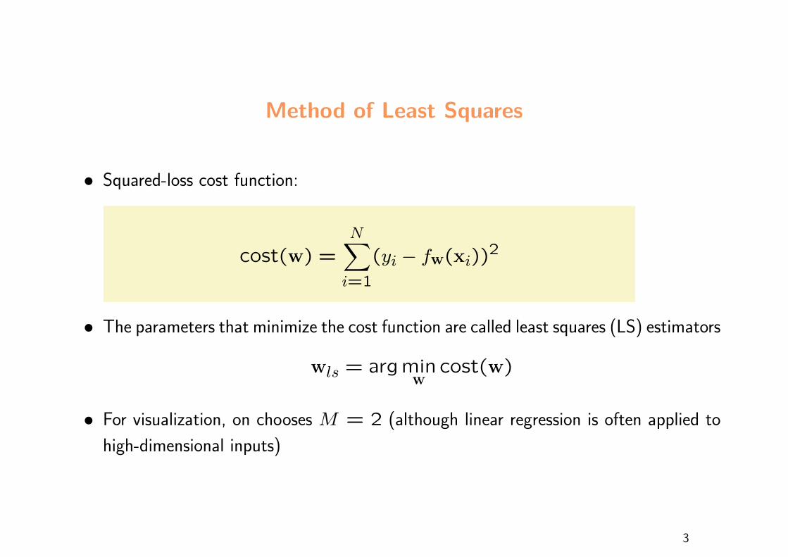
Method of Least Squares

• Squared-loss cost function:

cost(w) =N∑i=1

(yi − fw(xi))2

• The parameters that minimize the cost function are called least squares (LS) estimators

wls = argminw

cost(w)

• For visualization, on chooses M = 2 (although linear regression is often applied to

high-dimensional inputs)

3

Least-squares Estimator for Regression

One-dimensional regression:

fw(x) = w0 + w1x

w = (w0, w1)T

Squared error:

cost(w) =N∑i=1

(yi − fw(xi))2

Goal:

wls = argminw

cost(w) w0 = 1, w1 = 2, var(ε) = 1

4

Least-squares Estimator in General

General Model:

yi = f(xi,w) = w0 +M−1∑j=1

wjxi,j

= xTi w

w = (w0, w1, . . . wM−1)T

xi = (1, xi,1, . . . , xi,M−1)T

5

Linear Regression with Several Inputs

6

Contribution to the Cost Function of one Data Point

7

Gradient Descent Learning

• Initialize parameters (typically using small random numbers)

• Adapt the parameters in the direction of the negative gradient

• With

cost(w) =N∑i=1

yi −M−1∑j=0

wjxi,j

2

• The parameter gradient is (Example: wj)

∂cost

∂wj= −2

N∑i=1

(yi − fw(xi))xi,j

• A sensible learning rule is

wj ←− wj + η

N∑i=1

(yi − fw(xi))xi,j

8

ADALINE-Learning Rule

• ADALINE: ADAptive LINear Element

• The ADALINE uses stochastic gradient descent (SGE)

• Let xt and yt be the training pattern in iteration t. The we adapt, t = 1,2, . . .

wj ←− wj + η(yt − yt)xt,j j = 1,2, . . . ,M

• η > 0 is the learning rate, typically 0 < η << 0.1

• Compare: the Perceptron learning rule (only applied to misclassified patterns)

wj ←− wj + ηytxt,j j = 1, . . . ,M

9

Analytic Solution

• The least-squares solution can be calculated in one step

10

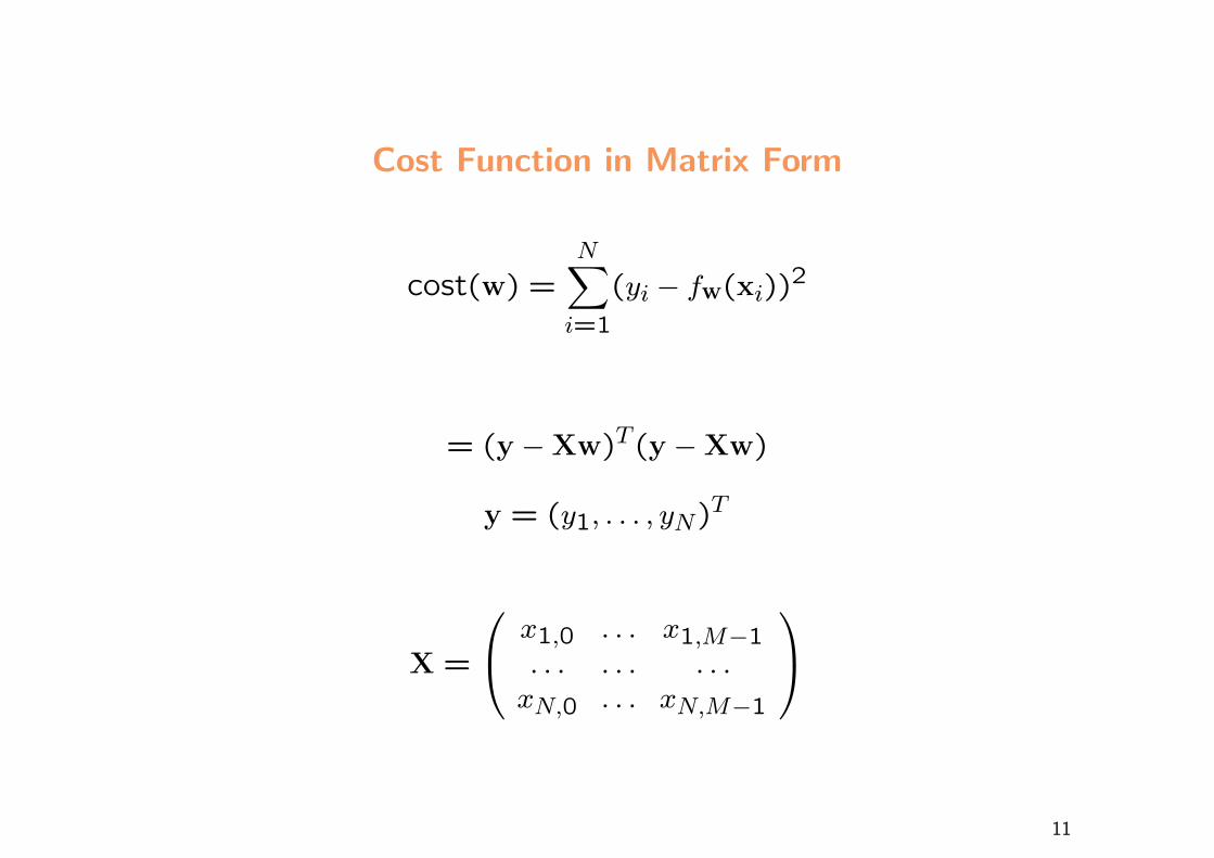
Cost Function in Matrix Form

cost(w) =N∑i=1

(yi − fw(xi))2

= (y −Xw)T (y −Xw)

y = (y1, . . . , yN)T

X =

x1,0 . . . x1,M−1. . . . . . . . .xN,0 . . . xN,M−1

11

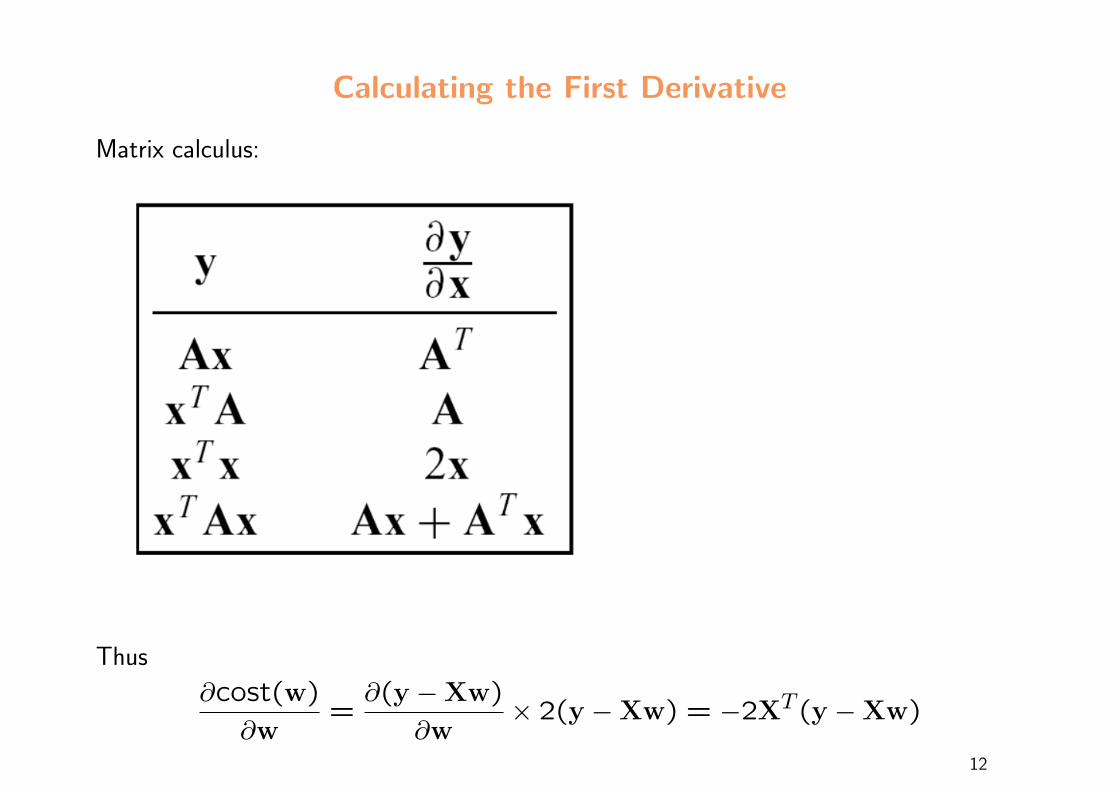
Calculating the First Derivative

Matrix calculus:

Thus

∂cost(w)

∂w=∂(y −Xw)

∂w× 2(y −Xw) = −2XT (y −Xw)

12

Setting First Derivative to Zero

Calculating the LS-solution:

∂cost(w)

∂w= −2XT (y −Xw) = 0

wls = (XTX)−1XTy

Complexity (linear in N !):

O(M3 +NM2)

w0 = 0.75, w1 = 2.13

13

Alternative Convention

Comment: one also finds the conventions:

∂

∂xAx = A

∂

∂xxTx = 2xT

∂

∂xxTAx = xT (A+AT )

Thus

∂cost(w)

∂w= 2(y −Xw)T ×

∂(y −Xw)

∂w= −2(y −Xw)TX

This leads to the same solution

14

Stability of the Solution

• When N >> M , the LS solution is stable (small changes in the data lead to small

changes in the parameter estimates)

• When N < M then there are many solutions which all produce zero training error

• Of all these solutions, one selects the one that minimizes∑Mi=0w

2i (regularised

solution)

• Even with N > M it is advantageous to regularize the solution, in particular with

noise on the target

15

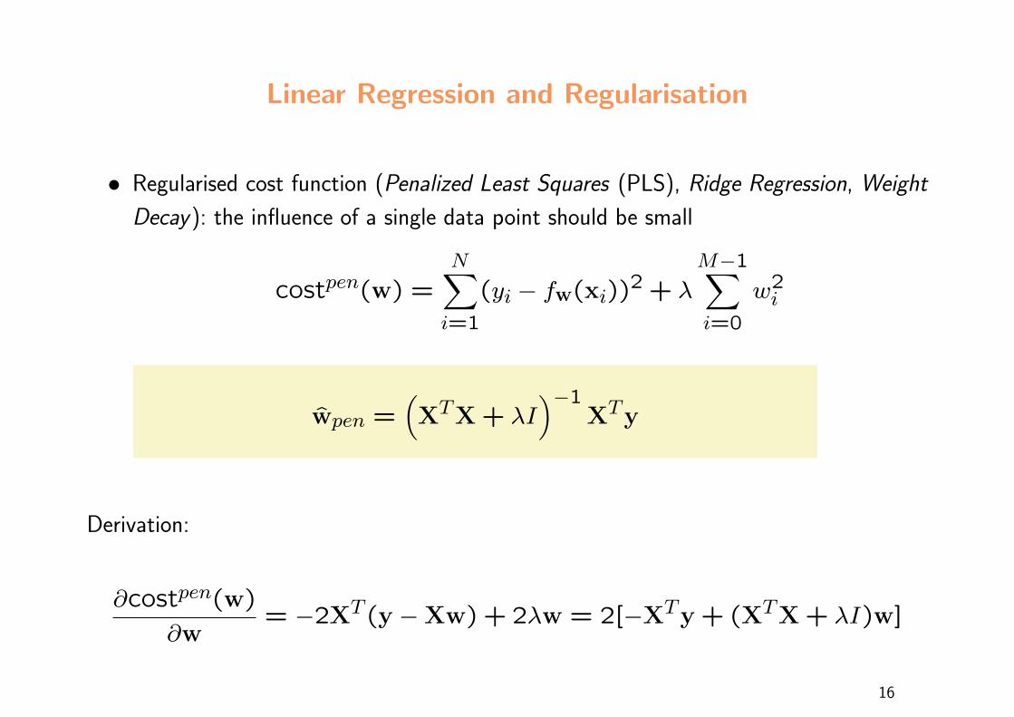
Linear Regression and Regularisation

• Regularised cost function (Penalized Least Squares (PLS), Ridge Regression, Weight

Decay): the influence of a single data point should be small

costpen(w) =N∑i=1

(yi − fw(xi))2 + λ

M−1∑i=0

w2i

wpen =(XTX+ λI

)−1XTy

Derivation:

∂costpen(w)

∂w= −2XT (y −Xw) + 2λw = 2[−XTy+ (XTX+ λI)w]

16

Example: Correlated Input with no Effect on Output(Redundant Input)

• Three data points are generated as (system; true model)

y = 0.5+ x1 + εi

Here, εi is independent noise

• Model 1 (correct structure)

fw(x) = w0 + w1x1

• Training data for Model 1:

x1 y

-0.2 0.490.2 0.641 1.39

• The LS solution gives wls = (0.58,0.77)T

17

• In comparison, the true parameters are: w = (0.50,1.00)T . The parameter esti-

mates are reasonable, considering that only three training patterns are available

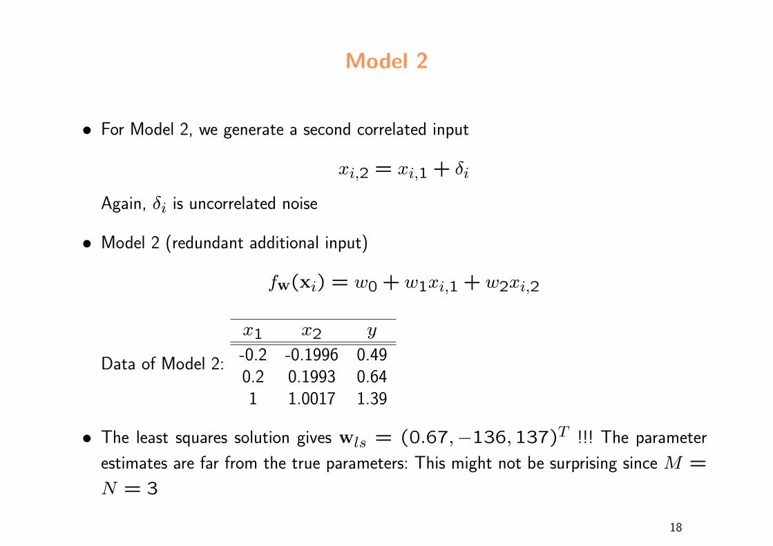
Model 2

• For Model 2, we generate a second correlated input

xi,2 = xi,1 + δi

Again, δi is uncorrelated noise

• Model 2 (redundant additional input)

fw(xi) = w0 + w1xi,1 + w2xi,2

Data of Model 2:

x1 x2 y

-0.2 -0.1996 0.490.2 0.1993 0.641 1.0017 1.39

• The least squares solution gives wls = (0.67,−136,137)T !!! The parameter

estimates are far from the true parameters: This might not be surprising since M =

N = 3

18

Model 2 with Regularisation

• As Model 2, only that large weights are penalized

• The penalized least squares solution gives wpen = (0.58,0.38,0.39)T , also

difficult to interpret !!!

• (Compare: the LS-solution for Model 1 gave wls = (0.58,0.77))T

19

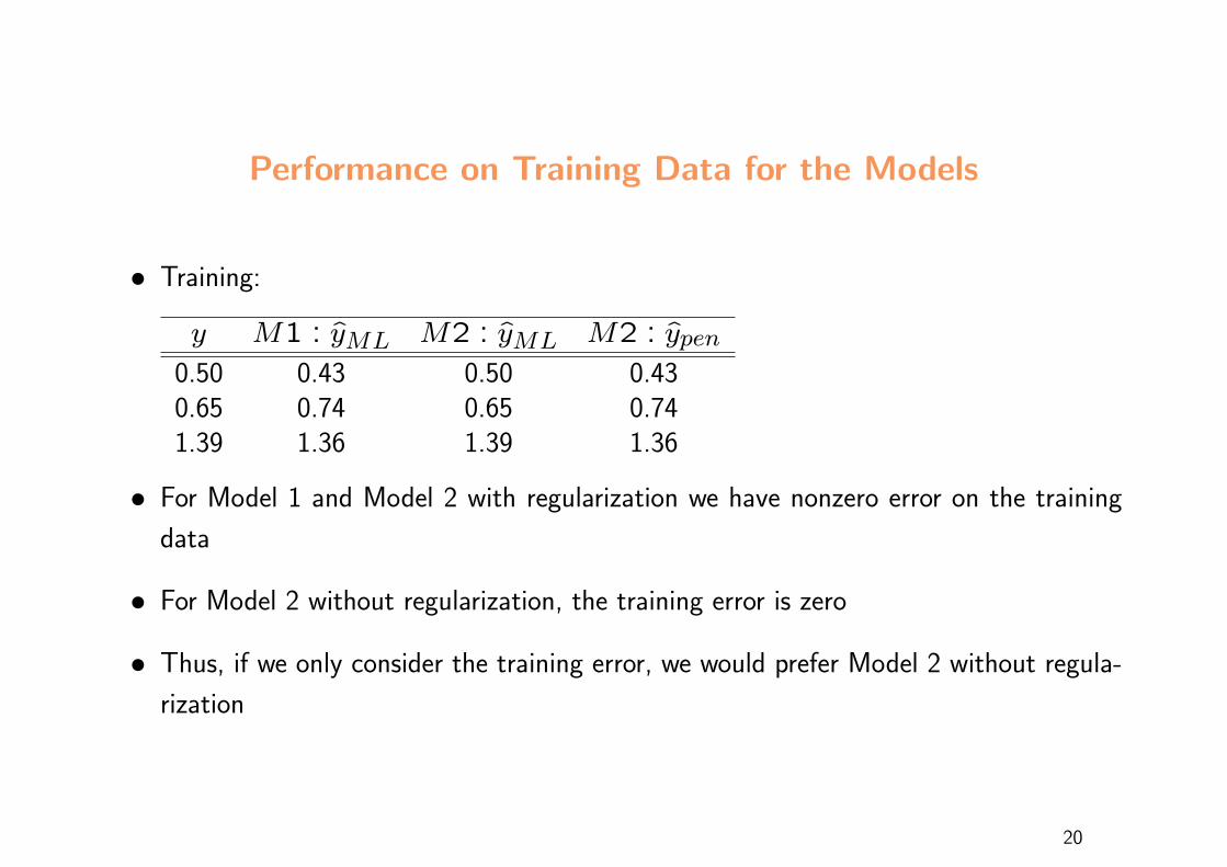
Performance on Training Data for the Models

• Training:

y M1 : yML M2 : yML M2 : ypen0.50 0.43 0.50 0.430.65 0.74 0.65 0.741.39 1.36 1.39 1.36

• For Model 1 and Model 2 with regularization we have nonzero error on the training

data

• For Model 2 without regularization, the training error is zero

• Thus, if we only consider the training error, we would prefer Model 2 without regula-

rization

20

Performance on Test Data for the Models

• Test Data:

y M1 : yML M2 : yML M2 : ypen0.20 0.36 0.69 0.360.80 0.82 0.51 0.821.10 1.05 1.30 1.05

• On test data Model 1 and Model 2 with regularization give better results

• Even more dramatic: extrapolation (not shown)

• As a conclusion: Model 1, which corresponds to the system performs best. For Model

2 (with additional correlated input) the penalized version gives best predictive results,

although the parameter values are difficult to interpret. Without regularization, the

prediction error of Model 2 on test data is large. Asymptotically, with N → ∞,

Model 2 might learn to ignore the second input and w0 and w1 converge to the

true parameters. Thus, regularization helps predictive performance but does

not lead to interpretable parameters, which is why it is not often used in

21

classical statistical analysis. In Machine Learning, where we care mostly

about predictive performance, regularization is the standard!

Experiments with Real World Data: Data from Prostate CancerPatients

8 Inputs, 97 data points; y: Prostate-specific antigen

10-times cross validation errorLS 0.586

Best Subset (3) 0.574Ridge (Penalized) 0.540

22

GWAS Study

Trait (here: the disease systemic sclerosis) is the output and the SNPs are the inputs. The

major allele is encoded as 0 and the minor allele as 1. Thus wj is the influence of SNP

j on the trait. Shown is the (log of the p-value) of wj ordered by the locations on the

chromosomes. The weights can be calculated by penalized least squares (ridge regression)

23