Linear Regression: Goodness of Fit andModel Selection

1

Goodness of Fit

I Goodness of fit measures for linear regression are attemptsto understand how well a model fits a given set of data.

I Models almost never describe the process that generated adataset exactly

I Models approximate reality

I However, even models that approximate reality can beused to draw useful inferences or to prediction futureobservations

I ’All Models are wrong, but some are useful’ - George Box

2

Goodness of Fit

I We have seen how to check the modelling assumptions oflinear regression:

I checking the linearity assumption

I checking for outliers

I checking the normality assumption

I checking the distribution of the residuals does not dependon the predictors

I These are essential qualitative checks of goodness of fit

3

Sample SizeI When making visual checks of data for goodness of fit is

important to consider sample size

I From a multiple regression model with 2 predictors:

I On the left is a histogram of the residuals

I On the right is residual vs predictor plot for each of thetwo predictors

4

Sample Size

I The histogram doesn’t look normal but there are only 20datapoint

I We should not expect a better visual fit

I Inferences from the linear model should be valid5

Outliers

I Often (particularly when a large dataset is large):I the majority of the residuals will satisfy the model

checking assumption

I a small number of residuals will violate the normalityassumption: they will be very big or very small

I Outliers are often generated by a process distinct fromthose which we are primarily interested in. i.e. theprocess generating the relationships between the responseand the predictors

I e.g. Outliers are often generated by measurement orexperimental errors

I In these circumstances, rather than reject the linear modeland search for a simpler one, it is usually better to removethe outliers from the dataset.

6

Outlier Detection

I Outliers can be detected graphically using the qqnormfunction:

7

Automatic Outlier Detection

I Automated outlier detection is built into R

I Apply the plot command to an R linear model object:> plot(lm(y∼ x))

8

Goodness of Fit

I Visual checks are important methods for checking thequality of the fit of a linear model to a dataset

I However they are qualitative, quantitative measure ofgoodness of fit are also important

I Quantitative measures allow us to compare the goodness offit of different models to the same dataset

9

Residual Sum of Squares (SSE)

I The residual sum of squares is defined as

SSE =

n∑i

r2i

=

n∑i

(Yi − α̂− β̂x)2

I This is a simple measure of goodness of fit

I The smaller the SSE the better the fit of the model

I Note SSE depends on n the number of data points, so itcannot be used to compare the quality of fit of models fitto datasets of different size.

10

R2

I You may have noticed that the R2 value is routinely givenin the R software output

I R2 is a measure of variance explained by the predictors

I We will now see how to define and interpret this measure.

11

R2

I Consider two equations models:

EYi = α+β× xi (1)

EYi = α (2)

I R2 of the first model is defined as:

1 −sum of squared residuals from model (2)sum of squared residuals from model (1)

I If better model (2) is at explaining the variation comparedto model (1). The closer R2 will be to 1.

12

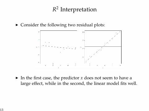
R2 Interpretation

I Consider the following two residual plots:

I In the first case, the predictor x does not seem to have alarge effect, while in the second, the linear model fits well.

13

R2 Properties

I R2 is a number between 0 and 1

I The R2 for a simple linear regression is the squaredcorrelation between x and Y

I The larger R2 the better the fit

I If you add a predictor to a multiple linear regression R2

always goes up

I This means R2 is inappropriate to compare the quality offit of models with different numbers of predictors

I More complex models always fit better

14

Model Selection

I Recall there are two main reasons for fitting a statisticalmodel

1 Scientific Inference: estimating an interpretable parameter

2 Prediction: if you give me a new x1, x2, ...xp can I predictthe value of the corresponding Y without seeing it.

I Models for making scientific inferences are not normallychosen using statistical ‘black box’ model selectionprocedures. Usually the choice of model(s) depends onthe scientific question and knowledge of the datagenerating process.

I Model selection methods are used primarily for findinggood models for making predictions.

15

Averaging Over Models

I Optimal predictions often come from averaging overpredictions from multiple models.

I In this lecture we will concentrate on methods for findinga single optimal model amongst a set of possibilities.

16

Complex Models are not Good for Prediction

I Problem: find a model using the current dataset that isgoing to be good at predicting a new observation.

I As we’ve seen we can move to a model with improvedgoodness of fit of by adding a new predictor to the currentmodel, so its easy to find a model which fits well to agiven dataset

I But really complex models aren’t necessarily good forpredicting new observtions, even if they are a good fit tothe current dataset.

17

Model Parsimony

I Measures of model parsimony take into account goodnessof fit to the data and model complexity.

I If two models have the same number of parameters theone with the better goodness of fit will be the moreparsimonious.

I If two models have the same goodness of fit (rarelyhappens) the model with the fewer parameters will be themore parsimonious.

I More parsimonious models should give better predictions(on average).

18

Measures of Model Parsimony

I There are many measures of model parsimony.

I We will concentrate on AIC and BIC.

19

AIC

I The formula for AIC is

n log SSE + 2p

I SSE is the residual sum of squares, this is a goodness of fitmeasure

I p is the number of parameters of the model (number ofregression coefficients).

I Smaller values of AIC correspond to more parsimoniousmodels.

I AIC tends to be liberal (i.e. can add in too manypredictors, overfit)

20

BIC

I The formula for BIC in linear regression is

2 log SSE + p log(n)

I n is the sample size.

I The complexity penalty is stronger than that for AIC.

I Smaller values of BIC correspond to more parsimoniousmodels.

I BIC tends to be conservative (i.e. it requires quite a bit ofevidence before it will include a predictor)

21

Number of Possible Regression Models

I If we have p predictors we can build 2p possible models.

I e.g. p = 2 the 2p = 22 = 4 possible linear regressionmodels have regression equations:

EYi= α

EYi = α+β1X1

EYi = α+β2X2

EYi= α+β1X1 +β2X2

I The blue model is called the empty model.

I The red model is called the saturated (or full) model.

22

All Subsets Selection

I All subsets selection is the simplest model searchalgorithm.

1 Choose a model parsimony criterion.

2 Fit each of the 2p models and compute the criterion.

3 Rank the models by the criterion and choose the mostparsimonious.

I On modern computers this is doable providing p is notmuch larger than a number in the late teens. 220 ≈ 1million.

23

Forward Selection

I This algorithm can be run with any model selectioncriterion.

I Start (usually) with the empty model as the current model.

I Iterate the following:1 Fit all the models you can generate by augmenting the

current model by one variable.

2 If none of the models fitted in 1 is ranked better by themodel selection criterion than the current model terminatethe algorithm and output the current model.

3 Update the current model with the model fitted in 1 thatis ranked best by the model selection criterion.

I This fits at most p(p + 1)/2 models (faster than 2p).

I May not always find the best model, once a variable is inthe model it can’t be removed.24

Backward Elimination

I This algorithm can be run with any model selectioncriterion.

I Start (usually) with the saturated model.

I Iterate the following:1 Fit all the models you can generate by reducing the current

model by one variable.

2 If none of the models fitted in 1 is ranked better by themodel selection criterion than the current model terminatethe algorithm and output the current model.

3 Update the current model with the model fitted in 1 thatis ranked best by the model selection criterion.

I This fits at most p(p + 1)/2 models (faster than 2p).

I May not always find the best model, once a variable is outof the model it can’t be returned.25

Combined Forward and Backwards Selection

I This algorithm can be run with any model selectioncriterion.

I Starting point not so important.

I Iterate the following:1 Fit all the models you can generate by augmenting or

reducing the current model by one variable.

2 If none of the models fitted in 1 is ranked better by themodel selection criterion than the current model terminatethe algorithm and output the current model.

3 Update the current model with the model fitted in 1 thatis ranked best by the model selection criterion.

I May not always find the best model, but more likely tothan forward selection or backward elimination.

26

R Example

I A dataset of 50 observations recording the height, weight,sex, age, number of children and number of pets of asample of adults.

I We will run forward selection and combined forwardselection/backwards elimination on the dataset to find agood fitting model.

I We will use AIC as the measure of model parsimony

I This can be done using the R function step

27