Linear ProgrammingWeek 5 & 6

3.1 Graphing Systems of Linear Inequalities in Two Variables

Graphing Linear Inequality

Graph 2x + 3y < 6.

EXAMPLE 1 Determine the solution set for the inequality 2x + 3y ≥ 6.

EXAMPLE 2 Graph x £ 1.

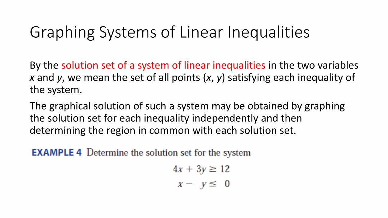
Graphing Systems of Linear Inequalities

By the solution set of a system of linear inequalities in the two variables x and y, we mean the set of all points (x, y) satisfying each inequality of the system.

The graphical solution of such a system may be obtained by graphing the solution set for each inequality independently and then determining the region in common with each solution set.

Bounded and Unbounded Solution Sets

The solution set of a system of linear inequalities is bounded if it can be

enclosed by a circle. Otherwise, it is unbounded.

3.2 Linear Programming Problems

Linear Programming Problems

In many business and economic problems, we are asked to optimize (maximize or minimize) a function subject to a system of equalities or inequalities. The function to be optimized is called the objective function.

Profit functions and cost functions are examples of objective functions.

The system of equalities or inequalities to which the objective function is subjected reflects the constraints (for example, limitations on resources such as materials and labor) imposed on the solution(s) to the problem.

Problems of this nature are called mathematical programming problems. In particular, problems in which both the objective function and the constraints are expressed as linear equations or inequalities are called linear programming problems.

A Maximization Problem

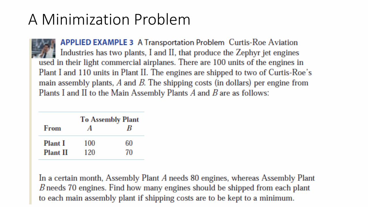
A Minimization Problem

3.3 Graphical Solution of Linear Programming Problems

The Graphical Method

The system of linear inequalities defines a planar region S.

Each point in S is a candidate for the solution of the problem at hand and is referred to as a feasible solution. The set S itself is referred to as a feasible set.

Our goal is to find, from among all the points in the set S, the point(s) that optimizes the objective

function P. Such a feasible solution is called an optimal solution and constitutes the

solution to the linear programming problem under consideration.

Linear Programming Theorems

THEOREM 1

If a linear programming problem has a solution, then it must occur at a vertex, or corner point, of the feasible set S associated with the problem.

Furthermore, if the objective function P is optimized at two adjacent vertices of S, then it is optimized at every point on the line segment joining these vertices, in which case there are infinitely many solutions to the problem.

THEOREM 2

Suppose we are given a linear programming problem with a feasible set S and an objective function P = ax + by.

a. If S is bounded, then P has both a maximum and a minimum value on S.

b. If S is unbounded and both a and b are nonnegative, then P has a minimum value on S provided that the constraints defining S include the inequalities x ≥ 0 and y ≥ 0.

c. If S is the empty set, then the linear programming problem has no solution; that is, P has neither a maximum nor a minimum value.

The Method of Corners

1. Graph the feasible set.

2. Find the coordinates of all corner points (vertices) of the feasible set.

3. Evaluate the objective function at each corner point.

4. Find the vertex that renders the objective function a maximum (minimum). If there is only one such vertex, then this vertex constitutes a unique solution to the problem. If the objective function is maximized (minimized) at two adjacent corner points of S, there are infinitely many optimal solutions given by the points on the line segment determined by these two vertices.

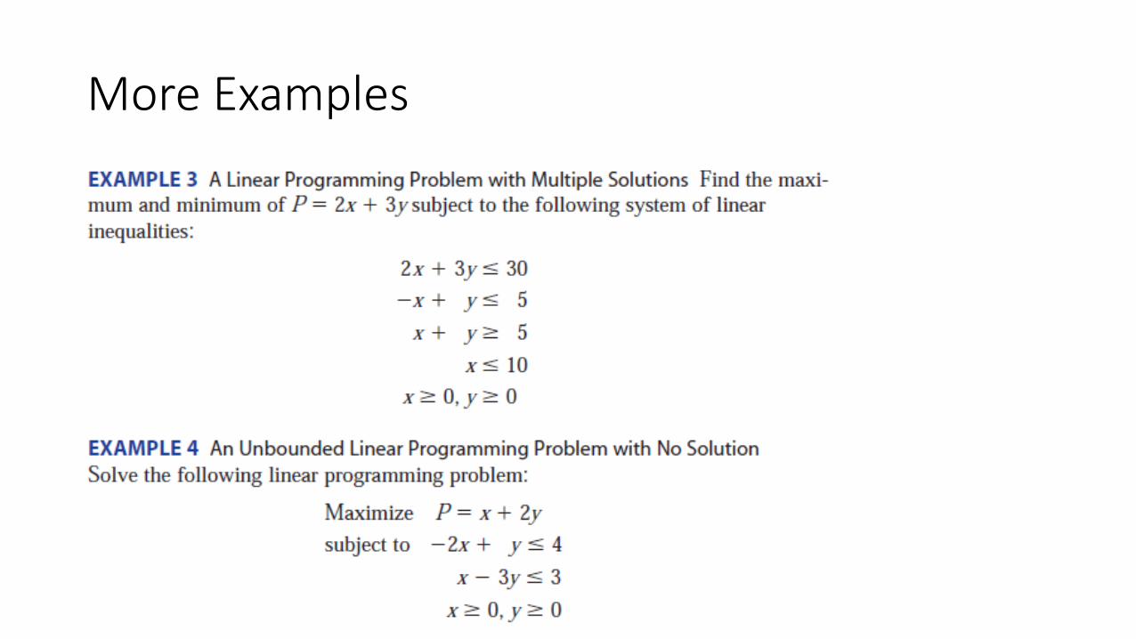
More Examples

A Maximization Problem

A Minimization Problem