Linear programming I

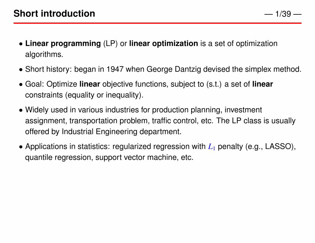
Short introduction — 1/39 —

• Linear programming (LP) or linear optimization is a set of optimizationalgorithms.

• Short history: began in 1947 when George Dantzig devised the simplex method.

• Goal: Optimize linear objective functions, subject to (s.t.) a set of linearconstraints (equality or inequality).

• Widely used in various industries for production planning, investmentassignment, transportation problem, traffic control, etc. The LP class is usuallyoffered by Industrial Engineering department.

• Applications in statistics: regularized regression with L1 penalty (e.g., LASSO),quantile regression, support vector machine, etc.

A simple motivating example — 2/39 —

Consider a hypothetical company that manufactures two products A and B.

1. Each item of product A requires 1 hour of labor and 2 units of materials, andyields a profit of 1 dollar.

2. Each item of product B requires 2 hours of labor and 1 unit of materials, andyields a profit of 1 dollar.

3. The company has 100 hours of labor and 100 units of materials available.

Question: what’s the company’s optimal strategy for production?

The problem can be formulated as following optimization problem. Denote theamount of production for product A and B by x1 and x2:

max z = x1 + x2,

s.t. x1 + 2x2 ≤ 1002x1 + x2 ≤ 100x1, x2 ≥ 0

Graphical representation — 3/39 —

The small, 2-variable problem can be represented in a 2D graph.The isoprofit line (any point on the line generate the same profit) is perpendicular tothe gradient of objective function. The problem can be solved by sliding the isoprofitline.

Properties of the optimal solution — 4/39 —

Optimal solution might not exist (e.g., the objective function is unbounded in thesolution space).But if the optimal solution exists:

• Interior point: NO.

• Corner point: Yes. The corner points are often referred to as “extreme points”.

• Edge point: Yes, only when the edge is parallel to the isoprofit line. In this case,every point on that edge has the same objective function value, including thecorner point of that edge.

• Key result: If an LP has an optimal solution, it must have a extreme pointoptimal solution (can be rigorously proved using the General RepresentationTheorem). This greatly reduce our search of optimal solutions: only need tocheck a finite number of extreme points.

The augmented LP — 5/39 —

The inequality constrains can be converted into equality constrains by addingnon-negative “slack” variables. For example,

x1 + 2x2 ≤ 100⇐⇒ x1 + 2x2 + x3 = 100, x3 ≥ 0.

Here x3 is called a “slack” variable.

The original problem can be expressed as the following slack form:

max z = x1 + x2,

s.t. x1 + 2x2 + x3 = 1002x1 + x2 + x4 = 100x1, x2, x3, x4 ≥ 0

This augmentation is necessary for simplex algorithm.

LP in matrix notation — 6/39 —

The augmented standard form of LP problem, expressed in matrix notation is:

max z = cxs.t. Ax = b

x ≥ 0

It is required that RHS b ≥ 0. Here x is augmented, e.g., including the original andslack variables. For our simple example, we have:

x = [x1, x2, x3, x4]T

c = [1, 1, 0, 0]

A =[

1 2 1 02 1 0 1

]b = [100, 100]T

Finding extreme points — 7/39 —

We know the problem has an optimal solution at the extreme point if the optimalsolution exists =⇒ we can try all extreme points and find the best one.

Assume there are m constraints an n unknowns (so A is of dimension m × n). In ourcase m = 2 and n = 4.

• It is required that m < n (why?)

• Assume rank(A) = m, e.g., rows of A are independent, or there’s no redundantconstraints.

• An extreme point is the intersection of n linearly independent hyperplanes. Theconstraints Ax = b provide m such hyperplanes. How about the remaining n − mof them?

Solution: first set n − m of the unknowns to zero. Essentially this gets rid of n − mvariables and leaves us with m unknowns and m equations, which can be solved.

Finding extreme points (cont.) — 8/39 —

Terminology: The n − m variables set to zero are called nonbasic variables (NBV)and denoted by xN. The rest m variables are basic variables (BV), denoted by xB.

Let B be the columns of A that are associated with the basic variables, and N bethe columns associated with nonbasic variables (B is square and has full rank):

Ax = b =⇒ [B,N][

xB

xN

]= b =⇒ xB = B−1b

So the point xN = 0, xB = B−1b is an extreme point.

Bad news: there are too many of them! With 20 variables and 10 constraints, there

are(

2010

)= 184, 756 extreme points.

Recognizing the optimal solution — 9/39 —

Given the LP problem

max z = cx, s.t. Ax = b, x ≥ 0

First characterize the solution at a extreme point:

BxB + NxN = b =⇒ xB = B−1b − B−1NxN =⇒ xB = B−1b −∑j∈R

B−1a jx j

Here R is the set of nonbasic variables, and a j’s are columns of A.

Substitute this expression to the objective function,

z = cx = cBxB + cNxN

= cB

B−1b −∑j∈R

B−1a jx j

+∑j∈R

c jx j

= cBB−1b −∑j∈R

(cBB−1a j − c j)x j

The current extreme point is optimal if cBB−1a j − c j ≥ 0 for ∀ j (why?).

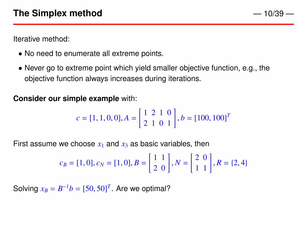
The Simplex method — 10/39 —

Iterative method:

• No need to enumerate all extreme points.

• Never go to extreme point which yield smaller objective function, e.g., theobjective function always increases during iterations.

Consider our simple example with:

c = [1, 1, 0, 0], A =[

1 2 1 02 1 0 1

], b = [100, 100]T

First assume we choose x1 and x3 as basic variables, then

cB = [1, 0], cN = [1, 0], B =[

1 12 0

],N =

[2 01 1

],R = {2, 4}

Solving xB = B−1b = [50, 50]T . Are we optimal?

— 11/39 —

Check cBB−1a j − c j ≡ w j for j ∈ R.

w2 = [1, 0][

1 12 0

]−1 [21

]− 1 = −0.5

w4 = [1, 0][

1 12 0

]−1 [01

]− 0 = 0.5

• w2 < 0 so we know the solution is not optimal =⇒ increasing x2 will increase theobjective function z.

• Since we will increase x2, it will no longer be a nonbasic variable (will not bezero). It is referred to as entering basic variable.

• But when we increase x2, it will change the values of other variables. How muchcan we increase x2?

— 12/39 —

Now go back to look at xB = B−1b −∑

j∈R B−1a jx j. To simplify the notations, definey j = B−1a j for j ∈ R, and b̄ = B−1b.

y2 = B−1a2 =

[1 12 0

]−1 [21

]=

[0.51.5

]y4 = B−1a4 =

[1 12 0

]−1 [01

]=

[0.5−0.5

]b̄ =

[1 12 0

]−1 [100100

]=

[5050

]

Plug these back to the expessions for xB:[x1

x3

]=

[5050

]−

[0.51.5

]x2 −

[0.5−0.5

]x4

Holding x4 = 0 and increasing x2, x1 or x3 will eventually become negative.

— 13/39 —

How much can we increase x2 =⇒ increasing x2, which basic variable (x1 and x3)will hit zero first?

The basic variable that hits zero first is called the leaving basic variable. Givenindex of entering basic variable k, we find index for the leaving basic variable,denoted by l, as following:

l = argmini

{b̄i

yki, 1 ≤ i ≤ m, yki > 0

}

For our example, k = 2, b̄1/y21 = 50/0.5 = 100, b̄2/y22 = 50/1.5 = 33.3. So thesecond basic variable is leaving, which is x3.

Be careful of the indexing here (especially in programming). It is the second ofthe current basic variable that is leaving, not x2!

— 14/39 —

Next iteration, with x1 and x2 as basic variables. We will have

cB = [1, 1], cN = [0, 0], B =[

1 22 1

],N =

[1 00 1

],R = {3, 4}

We will get xB = [33.3, 33.3]T , and

w3 = [1, 1][

1 22 1

]−1 [10

]− 0 = 0.33

w4 = [1, 1][

1 22 1

]−1 [01

]− 0 = 0.33

Both w’s are positive so we are at optimal solution now!

Summary of the Simplex method — 15/39 —

• It only considers extreme points.

• It moves as far as it can until the movement is blocked by another constraint.

• It’s greedy: find the edge that optimize the objective function the fastest andmove along that edge.

To make it formal, the steps for Simplex method are:

1. Randomly choose a set of basic variables (often use the slack variables).

2. Find entering basic variable. Define the set of nonbasic variable to be R. Foreach j ∈ R, compute CBB−1a j − c j ≡ ω j. If all ω j ≥ 0, the current solution isoptimal. Otherwise find k = argmin j∈Rω j, the kth nonbasic variable will be EBV.

3. Find leaving basic variable. Obtain l = argmini

{b̄iyki, 1 ≤ i ≤ m, yki > 0

}. The lth

current basic variable will be LBV.

4. Iterate steps 2 and 3.

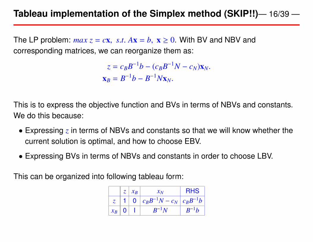
Tableau implementation of the Simplex method (SKIP!!)— 16/39 —

The LP problem: max z = cx, s.t. Ax = b, x ≥ 0. With BV and NBV andcorresponding matrices, we can reorganize them as:

z = cBB−1b − (cBB−1N − cN)xN.

xB = B−1b − B−1NxN.

This is to express the objective function and BVs in terms of NBVs and constants.We do this because:

• Expressing z in terms of NBVs and constants so that we will know whether thecurrent solution is optimal, and how to choose EBV.

• Expressing BVs in terms of NBVs and constants in order to choose LBV.

This can be organized into following tableau form:

z xB xN RHSz 1 0 cBB−1N − cN cBB−1bxB 0 I B−1N B−1b

Tableau implementation example (SKIP!!) — 17/39 —

The LP problem is:

max 50x1 + 30x2 + 40x3

s.t. 2x1 + 3x2 + 5x3 ≤ 1005x1 + 2x2 + 4x3 ≤ 80x1, x2, x3 ≥ 0

Step 1: Add slack variables (x4, x5) to get equality constraints.Step 2: Choose initial basic variables - the easiest is to choose the slack variablesas BV, then put into tableau (verify):

z x1 x2 x3 x4 x5 RHSz 1 -50 -30 -40 0 0 0x4 0 2 3 5 1 0 100x5 0 5 2 4 0 1 80

Choose x1 to be EBV (why?).

Step 3: Now to find LBV, need to compute ratios of the RHS column to the EBVcolumn, get x4 : 100/2, x5 : 80/5. We need to take the BV with minimum of theseratios, e.g., x5, as the LBV.Step 4: Update the tableau: replace x5 by x1 in BV. We must update the table sothat x1 has coefficient of 1 in row 2 and coefficient 0 in every other row. This step iscall pivoting.To do so, the new row 3 = old row 3 divided by 5:

z x1 x2 x3 x4 x5 RHSz 1x4 0x1 0 1 2/5 4/5 0 1/5 16

To eliminate the coefficient of x1 in row 1 and row 2, we perform row operations:

• new row 1 = old row 1 + 50 × new row 3.

• new row 2 = old row 2 − 2 × new row 3.

z x1 x2 x3 x4 x5 RHSz 1 0 -10 0 0 10 800x4 0 0 11/5 17/5 1 -2/5 68x1 0 1 2/5 4/5 0 1/5 16

Step 5: Now x2 will be EBV (because it has negative coefficient). By calculatingratios, x4 is LBV (verify!). Another step of pivoting gives:

z x1 x2 x3 x4 x5 RHSz 1 0 0 15 5

11 4 611 8 2

11 1109 111

x2 0 0 1 17/11 5/11 -2/11 301011

x1 0 1 0 2/11 -2/11 3/11 3 711

Now all coefficients for NBV are positive, meaning we have reached the optimalsolution.

The RHS column gives the optimal objective function value, as well as the values ofBVs at the optimal solution.

Handling ≥ constraints — 20/39 —

So far we assume all constraints are ≤ with non-negative RHS. What is someconstraints are ≥? For example, the following LP problem:

max − x1 − 3x2

s.t. x1 + 2x2 ≥ 15x1 + x2 ≤ 10x1, x2 ≥ 0

For the ≥ constraint we can subtract a slack variable (“surplus variable”):

max − x1 − 3x2

s.t. x1 + 2x2 − x3 = 15x1 + x2 + x4 = 10x1, x2, x3, x4 ≥ 0

The problem now is that we cannot use the slack variables as initial basic variableanymore because they are not feasible (why?).

Use artificial variables — 21/39 —

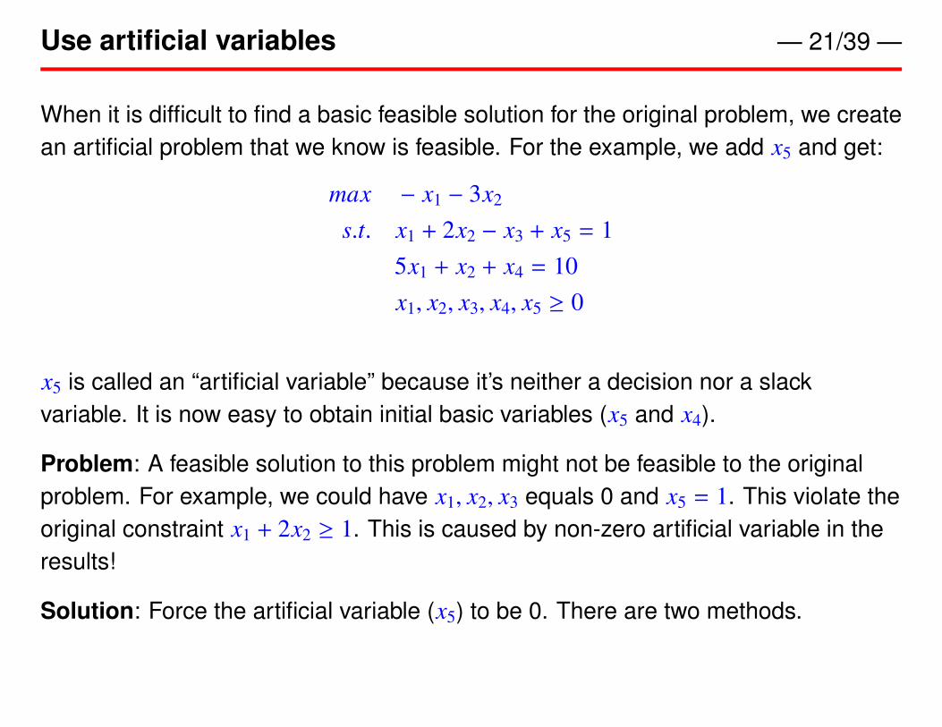
When it is difficult to find a basic feasible solution for the original problem, we createan artificial problem that we know is feasible. For the example, we add x5 and get:

max − x1 − 3x2

s.t. x1 + 2x2 − x3 + x5 = 15x1 + x2 + x4 = 10x1, x2, x3, x4, x5 ≥ 0

x5 is called an “artificial variable” because it’s neither a decision nor a slackvariable. It is now easy to obtain initial basic variables (x5 and x4).

Problem: A feasible solution to this problem might not be feasible to the originalproblem. For example, we could have x1, x2, x3 equals 0 and x5 = 1. This violate theoriginal constraint x1 + 2x2 ≥ 1. This is caused by non-zero artificial variable in theresults!

Solution: Force the artificial variable (x5) to be 0. There are two methods.

Two phase method — 22/39 —

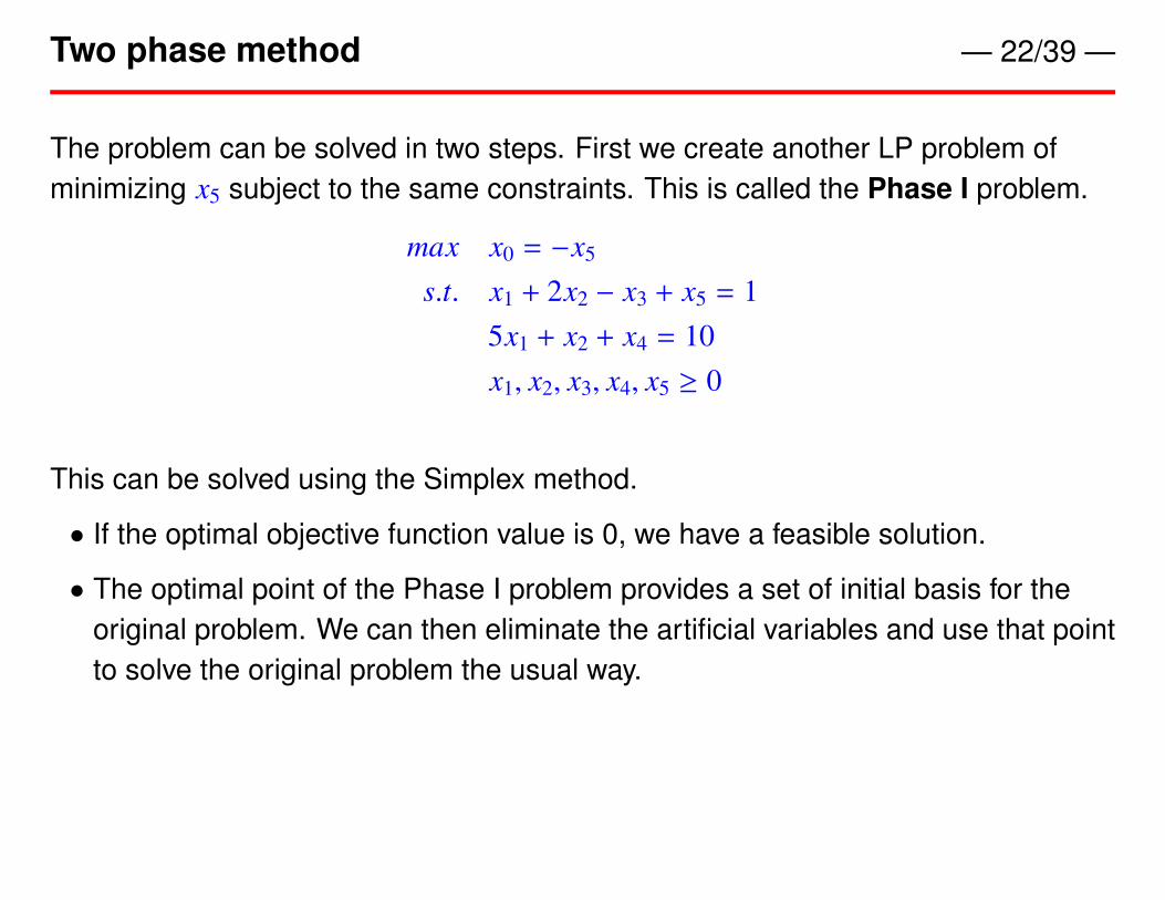
The problem can be solved in two steps. First we create another LP problem ofminimizing x5 subject to the same constraints. This is called the Phase I problem.

max x0 = −x5

s.t. x1 + 2x2 − x3 + x5 = 15x1 + x2 + x4 = 10x1, x2, x3, x4, x5 ≥ 0

This can be solved using the Simplex method.

• If the optimal objective function value is 0, we have a feasible solution.

• The optimal point of the Phase I problem provides a set of initial basis for theoriginal problem. We can then eliminate the artificial variables and use that pointto solve the original problem the usual way.

Put into tableau, get

x0 x1 x2 x3 x4 x5 RHSx0 1 0 0 0 0 1 0x5 0 1 2 -1 0 1 1x4 0 5 1 0 1 0 10

First eliminate the coefficient for artificial variables: new Row 1=Old row 1 - Old row2):

x0 x1 x2 x3 x4 x5 RHSx0 1 -1 -2 1 0 0 -1x5 0 1 2 -1 0 1 1x4 0 5 1 0 1 0 10

Pivot out x5, and pivot in x2, get:

x0 x1 x2 x3 x4 x5 RHSx0 1 0 0 0 0 1 0x2 0 1/2 1 -1/2 0 1/2 1/2x4 0 9/2 0 1/2 1 -1/2 19/2

Now x0 is optimized at x5 = 0. We can eliminate x5 and use x2 = 1/2, x4 = 19/2 asinitial solution for the original problem (this is the Phase II problem).The tableau for the initial problem is:

z x1 x2 x3 x4 RHSz 1 1 3 0 0 0x2 0 1/2 1 -1/2 0 1/2x4 0 9/2 0 1/2 1 19/2

This is not a valid tableau!! (why?)Need to adjust and get:

z x1 x2 x3 x4 RHSz 1 -1/2 0 3/2 0 -3/2x2 0 1/2 1 -1/2 0 1/2x4 0 9/2 0 1/2 1 19/2

Continue to finish!

The big-M method — 25/39 —

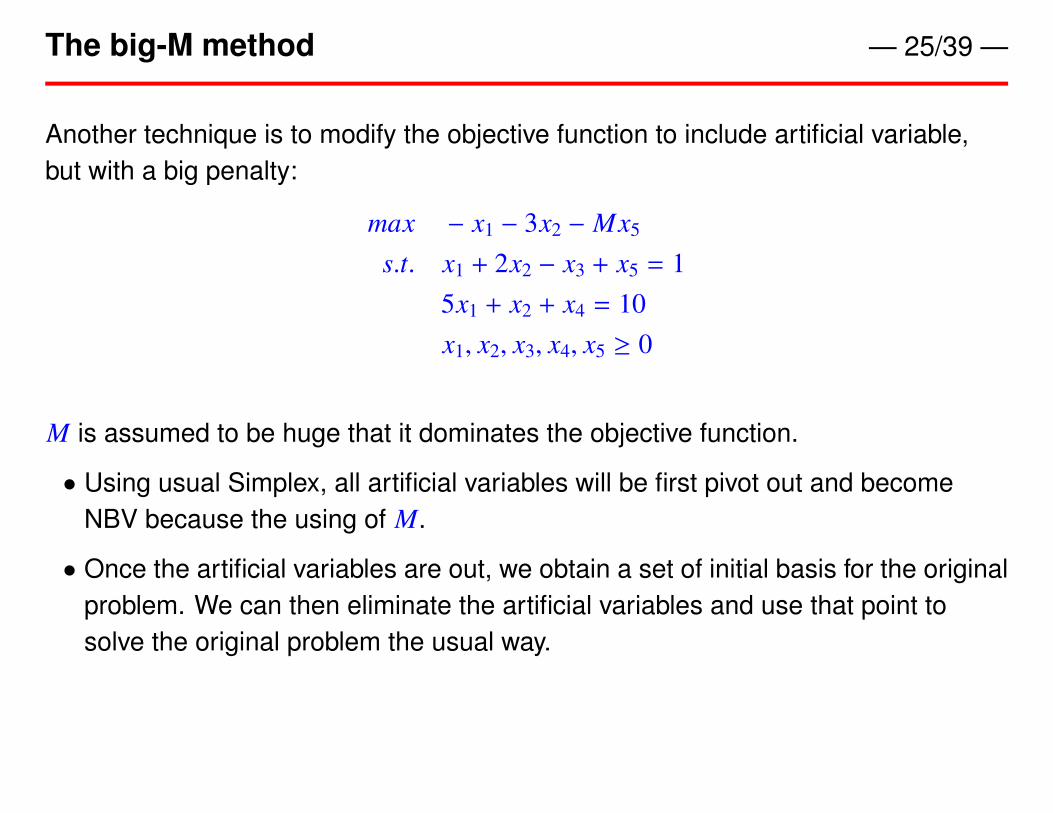
Another technique is to modify the objective function to include artificial variable,but with a big penalty:

max − x1 − 3x2 − Mx5

s.t. x1 + 2x2 − x3 + x5 = 15x1 + x2 + x4 = 10x1, x2, x3, x4, x5 ≥ 0

M is assumed to be huge that it dominates the objective function.

• Using usual Simplex, all artificial variables will be first pivot out and becomeNBV because the using of M.

• Once the artificial variables are out, we obtain a set of initial basis for the originalproblem. We can then eliminate the artificial variables and use that point tosolve the original problem the usual way.

Step for solving a general LP — 26/39 —

To solve a general LP with ≤, ≥ or = constraints:

1. Make all right hand size ≥ 0.

2. Add slack variables for ≤ constraints, and surplus variable for ≥ constraints.

3. Add artificial variables for ≥ or = constraints.

4. Use slack and artificial variables as initial basic variables.

5. Set up Phase I problem or use big-M method to pivot out all artificial variables(e.g., make all artificial variables nonbasic variables).

6. Use the optimal solution from Phase I or big-M as initial solution, eliminateartificial variables from the problem and finish the original problem.

LP solver software — 27/39 —

There are a large number of LP solver software both commercial or freely available.See Wikipedia page of “linear programming” for a list.

• In R, Simplex method is implemented as simplex function in boot package.

• In Matlab, the optimiztion toolbox contains linprog function.

• IBM ILOG CPLEX is commercial optimization package written in C. It is verypowerful and highly efficient for solving large scale LP problems.

Simplex method in R — 28/39 —

simplex package:boot R Documentation

Simplex Method for Linear Programming Problems

Description:

This function will optimize the linear function a%*%x subject to

the constraints A1%*%x <= b1, A2%*%x >= b2, A3%*%x = b3 and

x >= 0. Either maximization or minimization is possible but the

default is minimization.

Usage:

simplex(a, A1 = NULL, b1 = NULL, A2 = NULL, b2 = NULL, A3 = NULL,

b3 = NULL, maxi = FALSE, n.iter = n + 2 * m, eps = 1e-10)

Simplex Example in R — 29/39 —

> library(boot)

> a = c(50, 30, 40)

> A1 = matrix(c(2,3,5,5,2,4), nrow=2, byrow=TRUE)

> b1 = c(100, 80)

> simplex(-a, A1, b1)

Linear Programming Results

Call : simplex(a = -a, A1 = A1, b1 = b1)

Minimization Problem with Objective Function Coefficients

x1 x2 x3

-50 -30 -40

Optimal solution has the following values

x1 x2 x3

3.636364 30.909091 0.000000

The optimal value of the objective function is -1109.09090909091.

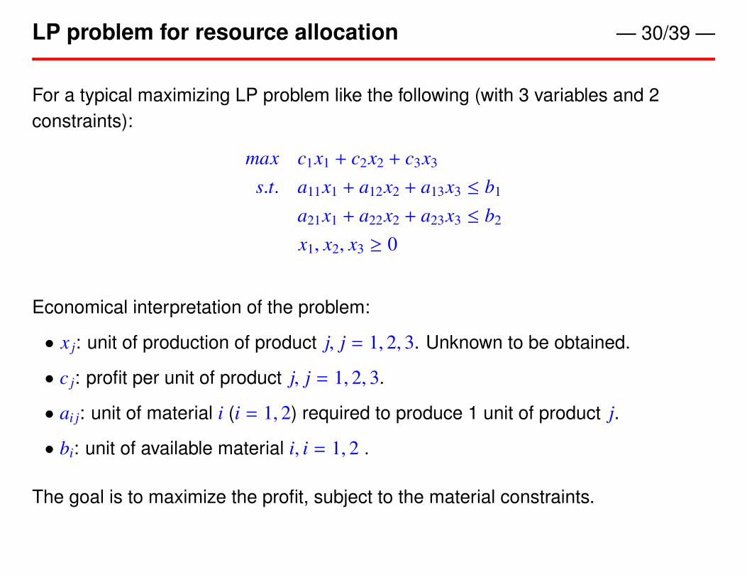
LP problem for resource allocation — 30/39 —

For a typical maximizing LP problem like the following (with 3 variables and 2constraints):

max c1x1 + c2x2 + c3x3

s.t. a11x1 + a12x2 + a13x3 ≤ b1

a21x1 + a22x2 + a23x3 ≤ b2

x1, x2, x3 ≥ 0

Economical interpretation of the problem:

• x j: unit of production of product j, j = 1, 2, 3. Unknown to be obtained.

• c j: profit per unit of product j, j = 1, 2, 3.

• ai j: unit of material i (i = 1, 2) required to produce 1 unit of product j.

• bi: unit of available material i, i = 1, 2 .

The goal is to maximize the profit, subject to the material constraints.

Resource valuation problem — 31/39 —

Now assume a buyer consider to buy our entire inventory of materials but not surehow to price the materials, but s/he knows that we will only do the business if sellingthe materials yields higher return than producing the product.

Buyer’s business strategy: producing one unit less of product j will save us:

• a1 j unit of material 1, and a2 j unit of material 2.

Buyer want to compute the unit prices of materials to minimize his/her cost, subjectto the constraints that we will do business (that we will not make less money).Assume the unit price for the materials are y1 and y2, the buyer will face thefollowing optimization problem (called Resource valuation problem):

min b1y1 + b2y2

s.t. a11y1 + a21y2 ≥ c1

a12y1 + a22y2 ≥ c2

a13y1 + a23y2 ≥ c3

y1, y2 ≥ 0

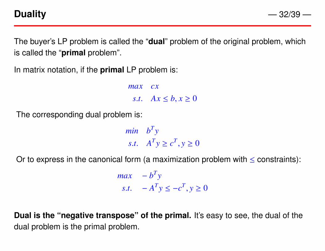
Duality — 32/39 —

The buyer’s LP problem is called the “dual” problem of the original problem, whichis called the “primal problem”.

In matrix notation, if the primal LP problem is:

max cxs.t. Ax ≤ b, x ≥ 0

The corresponding dual problem is:

min bT ys.t. AT y ≥ cT , y ≥ 0

Or to express in the canonical form (a maximization problem with ≤ constraints):

max − bT ys.t. − AT y ≤ −cT , y ≥ 0

Dual is the “negative transpose” of the primal. It’s easy to see, the dual of thedual problem is the primal problem.

Duality in non-canonical form — 33/39 —

What if the primal problem doesn’t fit into the canonical form (e.g., with ≥ or =constraints, unrestricted variable, etc.)? The general rules of converting are:

• The variable types of the dual problem is determined by the constraints types ofthe primal:

Primal (max) constraints Dual (min) variable≤ ≥ 0≥ ≤ 0= unrestricted

• The constraints types of the dual problem is determined by the variable types ofthe primal:

Primal (max) variable Dual (min) constraints≥ 0 ≥

≤ 0 ≤

unrestricted =

Examples of duality in non-canonical form — 34/39 —

If the primal problem is:

max 20x1 + 10x2 + 50x3

s.t. 3x1 + x2 + 9x3 ≤ 107x1 + 2x2 + 3x3 = 86x1 + x2 + 10x3 ≥ 1x1 ≥ 0, x2 unrestricted, x3 ≤ 0

The dual problem is:

min 10y1 + 8y2 + y3

s.t. 3y1 + 7y2 + 6y3 ≥ 20y1 + 2y2 + y3 = 109y1 + 3y2 + 10y3 ≤ 50y1 ≥ 0, y2 unrestricted, y3 ≤ 0

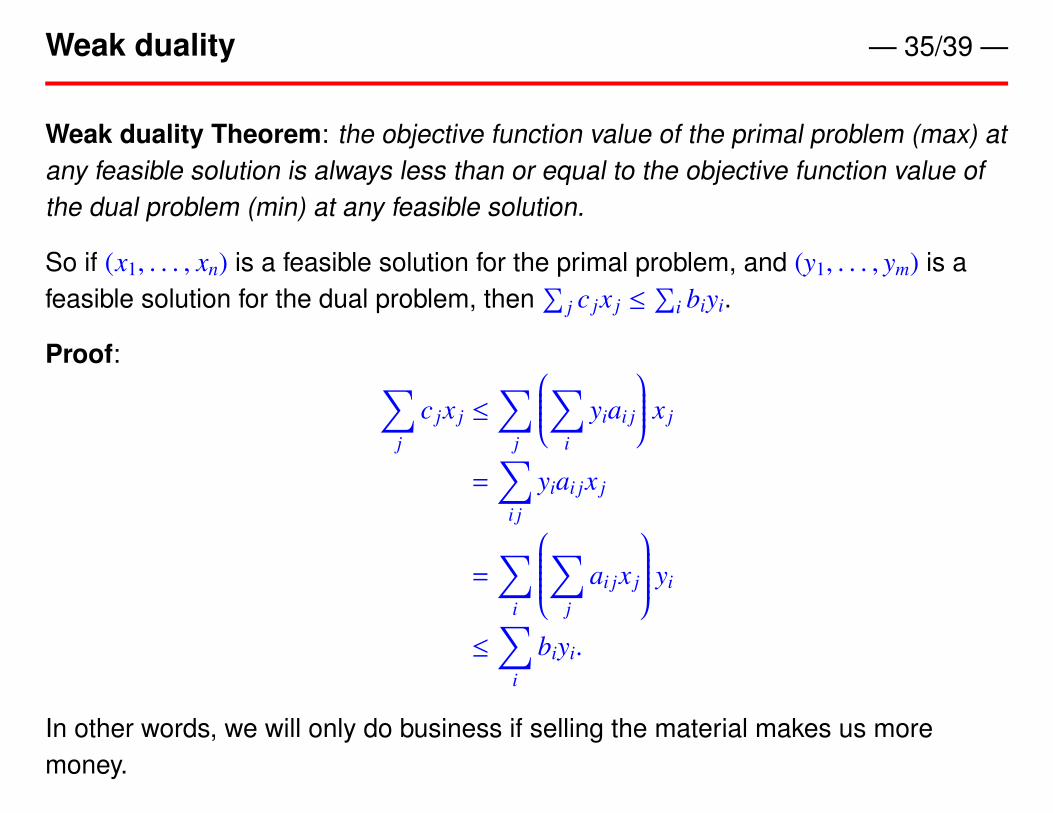
Weak duality — 35/39 —

Weak duality Theorem: the objective function value of the primal problem (max) atany feasible solution is always less than or equal to the objective function value ofthe dual problem (min) at any feasible solution.

So if (x1, . . . , xn) is a feasible solution for the primal problem, and (y1, . . . , ym) is afeasible solution for the dual problem, then

∑j c jx j ≤

∑i biyi.

Proof: ∑j

c jx j ≤∑

j

∑i

yiai j

x j

=∑

i j

yiai jx j

=∑

i

∑j

ai jx j

yi

≤∑

i

biyi.

In other words, we will only do business if selling the material makes us moremoney.

Strong duality — 36/39 —

• So we know now that at feasible solutions for both, the objective function of thedual problem is always greater or equal.

• A question is that if there is a difference between the largest primal value andthe smallest dual value? Such difference is called the “Duality gap”.

• The answer is provided by the following theorem.

Strong Duality Theorem: If the primal problem has an optimal solution, then thedual also has an optimal solution and there is no duality gap.

Economic interpretation: at optimality, the resource allocation and resourcevaluation problems give the same objective function values. In other words, in theideal economic situation, using the materials or selling the materials give the sameprofit.

Sketch of the proof (SKIP!) — 37/39 —

Recall for the LP problem in standard form: max z = cx, s.t. Ax ≤ b, x ≥ 0. Let x∗ bean optimal solution. Let B be the columns of A associated with the BV, and R is theset of columns associated with the NBV. We have cBB−1a j − c j ≥ 0 for ∀ j ∈ R.

• Define y∗ ≡ (cBB−1)T , we will have y∗T A ≥ c.

• Furthermore, y∗T ≥ 0 (why?).

Thus y∗ is a feasible solution for the dual problem.

How about optimality? We know y∗T b ≥ y∗T Ax ≥ cx. Want to prove y∗T b = cx∗. Thisrequires two steps:

1. y∗T b = y∗T Ax∗ ⇔ y∗T (b − Ax∗) = 0

2. y∗Ax∗ = cx∗ ⇔ (y∗T A − c)x∗ = 0

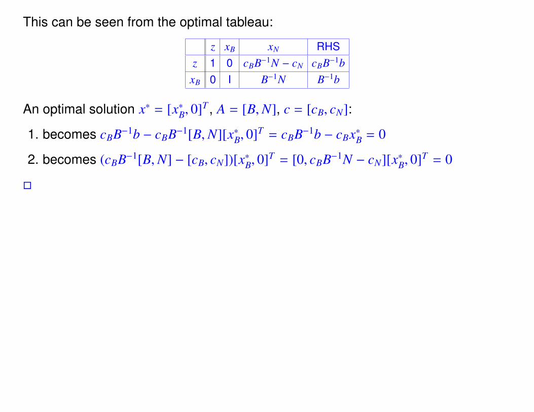
This can be seen from the optimal tableau:

z xB xN RHSz 1 0 cBB−1N − cN cBB−1bxB 0 I B−1N B−1b

An optimal solution x∗ = [x∗B, 0]T , A = [B,N], c = [cB, cN]:

1. becomes cBB−1b − cBB−1[B,N][x∗B, 0]T = cBB−1b − cBx∗B = 0

2. becomes (cBB−1[B,N] − [cB, cN])[x∗B, 0]T = [0, cBB−1N − cN][x∗B, 0]T = 0

�

Review — 39/39 —

• Linear programming (LP) is an constrained optimization method, where both theobjective function and constraints must be linear.

• If an LP has an optimal solution, it must have an extreme point optimal solution.This great reduces the search space.

• Simplex is a method to search for an optimal solution. It goes through theextreme points and guarantees the increase of objective function at every step.It has better performance than exhaustive search the extreme points.

• Primal–dual property of the LP.

• Weak and strong duality.